Luttinger Liquid and Polaronic Effects in Electron Transport through a Molecular Transistor

Abstract

Electron transport through a single-level quantum dot weakly coupled to Luttinger liquid leads is considered in the master equation approach. It is shown that for a weak or moderately strong interaction the differential conductance demonstrates resonant-like behavior as a function of bias and gate voltages. The inelastic channels associated with vibron-assisted electron tunnelling can even dominate electron transport for a certain region of interaction strength. In the limit of strong interaction resonant behavior disappears and the differential conductance scales as a power low on temperature (linear regime) or on bias voltage (nonlinear regime).

I Introduction

Last years electron transport in molecular transistors became a hot topic of experimental and theoretical investigations in nanoelectronics (see e.g. 1 ; 2 ). From experimental point of view it is a real challenge to place a single molecule in a gap between electric leads and to repeatedly measure electric current as a function of bias and gate voltages. Being in a gap the molecule may form chemical bonds with one of metallic electrodes and then a considerable charge transfer from the electrode to the molecule takes place. In this case one can consider the trapped molecule as a part of metallic electrode and the corresponding device does not function as a single electron transistor (SET). Much more interesting situation is the case when the trapped molecule is more or less isolated from the leads and preserves its electronic structure. In a stable state at zero gate voltage the molecule is electrically neutral and the chemical potential of the leads lies inside the gap between HOMO (highest occupied molecular orbital) and LUMO (lowest unoccupied molecular orbital) states. This structure demonstrates Coulomb blockade phenomenon 3 ; 4 and Coulomb blockade oscillations of conductance as a function of gate voltage (see review papers in 5 and references therein). In other words a molecule trapped in a potential well between the leads behaves as a quantum dot and the corresponding device exhibits the properties of SET. The new features in a charge transport through molecular transistors as compared to the well-studied semiconducting SET appear due to ”movable” character of the molecule trapped in potential well (the middle electrode of the molecular transistor). Two qualitatively new effects were predicted for molecular transistors: (i) vibron-assisted electron tunnelling (see e.g. 6 ; 7 ) and, (ii) electron shuttling 8 (see also review 9 ).

Vibron(phonon)-assisted electron tunnelling is induced by the interaction of charge density on the dot with local phonon modes (vibrons) which describe low-energy excitations of the molecule in a potential well. This interaction leads to satellite peaks (side bands) and unusual temperature dependence of peak conductance in resonant electron tunnelling 10 . For strong electron-vibron interaction the exponential narrowing of level width and as a result strong suppression of electron transport (polaronic blockade) was predicted 10 ; 11 . The effect of electron shuttling appears at finite bias voltages when additionally to electron-vibron interaction one takes into account coordinate dependence of electron tunnelling amplitude 8 ; 9 .

Recent years carbon nanotubes are considered as the most promising candidates for basic element of future nanoelectronics. Both $C_{60}$-based and carbon nanotube-based molecular transistors were already realized in experiment 12 ; 13 . The low-energy features of I-V characteristics measured in experiment with $C_{60}$-based molecular transistor 12 can be theoretically explained by the effects of vibron-assisted tunnelling 7 .

It is well known that in single-wall carbon nanotubes (SWNT) electron-electron interaction is strong and the electron transport in SWNT quantum wires is described by Luttinger liquid theory. Resonant electron tunnelling through a quantum dot weakly coupled to Luttinger liquid leads for the first time was studied in Ref.14 were a new temperature scaling of maximum conductance was predicted: $G(T)\propto T^{1/g-2}$ with interaction dependent exponent (g is the Luttinger liquid correlation parameter).

In this paper we generalize the results of Refs.10 ; 14 to the case when a quantum dot with vibrational degrees of freedom is coupled to Luttinger liquid quantum wires. The experimental realization of our model system could be, for instance, $C_{60}$-based molecular transistors with SWNT quantum wires.

In our model electron-electron and electron-phonon interactions can be of arbitrary strength while electron tunnelling amplitudes are assumed to be small (that is the vibrating quantum dot is weakly coupled to quantum wires). We will use master equation approach to evaluate the average current and noise power. For noninteracting electrons this approximation is valid for temperatures $T\gg\Gamma_{0}$, where $\Gamma_{0}$ is the bare level width. For interacting electrons the validity of this approach (perturbation theory on $\Gamma_{0}$) for high-T regime of electron transport was proved for $g<1/2$ (strong interaction) 15 and when $1-g\ll 1$ (weak interaction) 16 .

We found that at low temperatures: $\Gamma_{0}\ll T\ll\hbar w_{0}$ ($\hbar w_{0}$ is the characteristic energy of vibrons) the peak conductance scales with temperature accordingly to Furusaki prediction 14 : $G(T)\propto(\Gamma_{\lambda}/T)(T/\Lambda)^{1/g-1}$ ($\Lambda\simeq\varepsilon_{F}$ is the Luttinger liquid cutoff energy). The influence of electron-phonon interaction in low-T region results in renormalization of bare level width: $\Gamma_{\lambda}=\Gamma_{0}\exp(-\lambda^{2})$, where $\lambda$ is the dimensionless constant of electron-phonon interaction. In the intermediate temperature region: $\hbar w_{0}\leq T\leq\lambda^{2}\hbar w_{0}$, ($\lambda\gg 1$), Furusaki scaling is changed to $G(T)\propto(T)^{1/g-3/2}$ and at high temperatures when all inelastic channels for electron tunnelling are open we again recovered Furusaki scaling with nonrenormalized level width ($\Gamma_{0}$).

For nonlinear regime of electron tunnelling we showed that zero-bias peak in differential conductance, presenting elastic tunnelling, is suppressed by Coulomb correlations in the leads. This is manifestation of the Kane-Fisher effect 14 ; 15 . When interaction is moderately strong ($1/2\leq g<1$) the dependence of differential conductance on bias voltage is non-monotonous due to the presence of satellite peaks. For $g>1/2$ the zero-bias peak can be even more suppressed than the satellite peaks, which dominate in this case. This is the manifestation of the interplay between the Luttinger liquid effects in the leads and the electron-phonon coupling in the dot . For strong interaction $g<1/2$ satellites are also suppressed and the differential conductance at low temperatures ($T\ll\hbar w_{0}$) scales as $dI/dV\propto V^{1/g-2}$. This scaling coincides with the Furusaki prediction, where temperature is replaced by the driving voltage ($eV$) which becomes the relevant energy scale for $eV\gg T,\hbar w_{0},\Gamma$. It means that the influence of vibrons on the resonant electron tunnelling through a vibrating quantum dot can be observed only for weak or medium strong interaction ($1/2<g<1$) in the leads.

II The Model

The Hamiltonian of our system (vibrating quantum dot weakly coupled to Luttinger liquid leads, (see Fig.1) consists of three parts

$${\cal H}={\cal H}_{LL}+{\cal H}_{QD}+{\cal H}_{T}\ .$$ (1)

Here ${\cal H}_{LL}=\sum_{j=L,R}{\cal H}_{l}^{(j)}$ describes quantum wires adiabatically connected to electron reservoirs. Quantum wires (left-L and right-R) are supposed equal and modelled by Luttinger liquid Hamiltonians with equal Luttinger liquid parameters $1/g_{L(R)}$: $1/g_{L}=1/g_{R}=1/g$ (see e.g.14 )

$${\cal H}_{l}^{L(R)}={\cal H}_{l}=\hbar v_{c}\int_{0}^{\infty}a_{k}^{+}a_{k}kdk\ .$$ (2)

Here $a_{k}^{+}$($a_{k}$) are the creation (annihilation) operators of bosons which describe the charge density fluctuations propagating in the leads with velocity $v_{c}\sim v_{F}$. These operators satisfy canonical bosonic commutation relations $[a_{k},a_{k^{\prime}}^{+}]=\delta(k-k^{\prime})$. In what follows we consider for simplicity the case of spinless electrons.

The Hamiltonian of vibrating single level quantum dot takes the form (see e.g.10 )

$${\cal H}_{QD}=\varepsilon_{0}f^{+}f+\varepsilon_{i}(b^{+}+b)f^{+}f+\hbar w_{0}b^{+}b\ ,$$ (3)

where $\varepsilon_{0}$ is the energy of electron level on the dot, $\hbar w_{0}$ is the energy of vibrons, $\varepsilon_{i}$ is the electron-vibron interaction energy, $f^{+}$($f$) and $b^{+}$($b$) are fermionic ($f$) and bosonic ($b$) creation (annihilation) operators with canonical commutation relations $\{f,f^{+}\}=1$, $[b,b^{+}]=1$.

The tunnelling Hamiltonian is given by standard expression

$${\cal H}_{T}=\sum_{j=L,R}\{t_{j}f^{+}\Psi(j)+h.c.\}\ ,$$ (4)

where $t_{j}$ is the electron tunnelling amplitude and $\Psi(j)$, $j=L,R$ is the annihilation operator of electron at the end point of L(R)-electrode. This operator could be written in a ”bosonised” form (according to 14 )

$$\Psi(L(R))=\sqrt{\frac{2}{\pi\alpha}}\cdot\exp\left[\int_{0}^{\infty}dk\frac{e^{-\alpha k/2}}{\sqrt{2K_{\rho}k}}\cdot(a_{k}-a_{k}^{+})\right]\ ,$$ (5)

Here $\alpha$ is a short-distance cutoff of the order of the reciprocal of the Fermi wave number $k_{F}$ and $K_{\rho}=(2/g-1)^{-1}$ is the interaction parameter in the ”fermionic” form of the Luttinger liquid Hamiltonian (2), it defines the Luttinger liquid parameter $g$ which is varied between $0$ and $1$: the case $g=1$ describes the ”noninteracting” (Fermi-liquid) leads, than in the case $g\rightarrow 1$ the interaction in the leads goes to infinity.

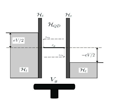
Figure 1: The schematic picture of the two-terminal electron transport through a vibrating quantum dot weakly coupled (via narrow dielectric regions $H_{t}$) to the Luttinger liquid leads (${\cal H}_{l}^{L(R)}={\cal H}_{l}$) with the chemical potentials $\varepsilon_{F}\pm eV/2$ ($V$ is the driving voltage). All the energies are counted from the Fermi energy, which chosen to be zero. Electrons tunnel from one lead to another by hopping on and off the dot level with the energy $\varepsilon_{P}$ (elastic channel) and due to electron-vibron coupling they can emit or absorb vibrons (vibron-assisted tunnelling). Inelastic channels are represented as side-levels with energies $\varepsilon_{P\pm}=\varepsilon_{P}\pm\hbar\omega_{0}$. The position of the dot levels with respect to the Fermi energy can be uniformly shifted by applying voltage $V_{g}$ to the ”gate” electrode.

Hamiltonian (3) is ”diagonalized” to ${\cal H}_{d}=\varepsilon_{P}f^{+}f+\hbar w_{0}b^{+}b$ by the unitary transformation (see e.g. 17 ) $U=\exp(i\lambda pn_{f})$, where $p=i(b^{+}-b)/\sqrt{2}$, $n_{f}=f^{+}f$ and the dimensionless parameter $\lambda=-\sqrt{2}\varepsilon_{i}/\hbar w_{0}$ characterizes electron-vibron coupling. The unitary transformation results in: (i) the shift of fermionic level (polaronic shift) $\varepsilon_{P}=\varepsilon_{0}-\varepsilon_{i}^{2}/\hbar w_{0}$ and, (ii) the replacement of tunnelling amplitude in (3) $t_{j}\Rightarrow t_{j}\cdot\exp(-i\lambda\cdot p)$. The model Eqs.(1)-(5)can not be solved exactly and one needs to exploit certain approximations to go further.

We will use ”master equation” approximation (see e.g. 5 ) to evaluate the average current and noise power in our model. It is in this approximation that average current separately for the model with interacting leads 14 and for vibrating quantum dot with noninteracting leads 18 was calculated earlier. Master (rate) equation approach exploits such quantities as the probability for electron to occupy dot level and the transition rates. It neglects quantum interference in electron tunnelling and therefore describes only the regime of sequential electron tunnelling which is valid when the width of electron level $\Gamma_{0}\ll\min(T,eV)$ . In other words, in our case ”master equation” approach is equivalent to the lowest order of perturbation theory in $\Gamma_{0}$.

For interacting electrons the validity of master equation approach for high-T regime of resonant electron tunnelling can be justified for strong repulsive interaction $g<1/2$ 14 . It is correct also for weak interaction $1-g\ll 1$ as one can check by comparing the results of Ref.14 and Ref. 16 , where resonant tunnelling through a double-barrier Luttinger liquid was considered for weak electron-electron interaction. Notice, that the results 18 of exact solution known for $g=1/2$, where a mapping to free-fermion theory can be used 5 , do not agree with the high-T scaling of $G(T)$ 14 extrapolated to this special point $g=1/2$. The free-fermion scaling $G(T)\propto T^{-1}$ found for $g=1/2$ (master equation approach predicts $T$-independent value 14 ) could be a special feature of this exactly solvable case. We will assume that beyond the close vicinity to $g=1/2$ the master equation approach for high-T behavior of conductance is a reasonable approximation.

III Transition rates and the average current

In master equation approach the average current through a single level quantum dot expressed in terms of transition rates takes the form

$$I=e\frac{\Gamma_{01}^{R}\Gamma_{10}^{L}-\Gamma_{01}^{L}\Gamma_{10}^{R}}{\Gamma_{\Sigma}}\ ,$$ (6)

where $\Gamma_{01}^{R(L)}$ is the rate of electron tunnelling from the dot to right (left) electrode, $\Gamma_{10}^{R(L)}$ describes the reverse process and $\Gamma_{\Sigma}=\Gamma_{01}+\Gamma_{10}$ , $\Gamma_{if}=\Gamma_{if}^{L}+\Gamma_{if}^{R}$ $(i,f=0,1)$. To evaluate these rates in our approach we will use Fermi ”Golden Rule” (quantum mechanical perturbation theory) for tunnelling Hamiltonian obtained from Eq.(4) after the unitary transformation: ${\cal H}_{T}\Rightarrow{\cal H}_{t}$

$${\cal H}_{t}=\sum_{j=L,R}\{t_{j}\Psi^{+}(j)f\exp(-i\lambda\cdot p)+h.c.\}\ .$$ (7)

The standard calculation procedure results in the following expressions for tunnelling rates

$$\Gamma_{10}^{(j)}=\left|\frac{t_{j}}{\hbar}\right|^{2}\int_{-\infty}^{\infty}dt\langle V(t)V^{+}(0)\rangle_{b}\langle\Psi_{j}^{+}(t)\Psi_{j}(0)\rangle_{f}$$

$$\cdot\exp(i(\varepsilon_{P}-\varepsilon_{F}+eV_{j})t/\hbar)\ ,$$ (8)

$$\Gamma_{01}^{(j)}=\left|\frac{t_{j}}{\hbar}\right|^{2}\int_{-\infty}^{\infty}dt\langle V^{+}(t)V(0)\rangle_{b}\langle\Psi_{j}(t)\Psi_{j}^{+}(0)\rangle_{f}$$

$$\cdot\exp(-i(\varepsilon_{P}-\varepsilon_{F}+eV_{j})t/\hbar)\ ,$$ (9)

where $V_{L}-V_{R}=V$ is the bias voltage and $j=L,R$. Notice that in the perturbation calculation on the bare level width $\Gamma_{0}\propto|t_{L,R}|^{2}$, we neglect the level width in the Green function of the dot level. Besides, in this approximation averages over bosonic and fermionic operators in formulas for tunnelling rates are factorized and, thus, the averages $\langle\ldots\rangle_{b}$ over bosonic variables

$$V=\exp(-i\lambda\cdot p)\ ,\ \ \ p=\frac{i}{\sqrt{2}}[b^{+}-b]$$ (10)

can be calculated with the quadratic Hamiltonian ${\cal H}_{b}=\hbar w_{0}b^{+}b$. In what follows we will assume that vibrons are characterized by equilibrium distribution function: $n_{b}(T)=[\exp(\hbar w_{0}/T)-1]^{-1}$. Averages $\langle\ldots\rangle_{f}$ over fermionic operators in Eqs.(8),(9) are calculated with the Luttinger liquid Hamiltonian (2). The corresponding correlation functions in Eqs.(8),(9) are well known in the literature (see e.g.10 ; 14 )

$$\langle V(t)V^{+}(0)\rangle_{b}=\exp(-\lambda^{2}(1+2n_{B}))$$

$$\cdot\left\{\sum_{l=-\infty}^{\infty}I_{l}\left[2\lambda^{2}\sqrt{n_{B}(1+n_{B})}\right]\exp[-ilw_{0}(t+i\hbar/2T)]\right\}$$

$$\langle\Psi_{j}^{+}(t)\Psi_{j}(0)\rangle_{f}\simeq\frac{\Lambda}{\hbar v_{F}}\cdot\left\{\frac{i\Lambda}{\pi T}\cdot\sinh\left[\frac{\pi T\cdot t}{\hbar}\right]\right\}^{-1/g}\ .$$ (12)

Here $I_{l}(z)$ is a modified Bessel function, $\Lambda\sim\varepsilon_{F}$ is a ultraviolet cutoff energy, $g$ is the Luttinger liquid correlation parameter.

By putting correlation functions (11),(12) in Eqs.(8),(9) and evaluating time integrals we get the following equations for tunnelling rates $\Gamma^{(j)}_{+}=\Gamma^{(j)}_{10}$ and $\Gamma^{(j)}_{-}=\Gamma^{(j)}_{01}$, ($j=L,R$)

$$\Gamma^{(j)}_{\pm}=\frac{\Gamma_{j}}{2\pi\hbar}\frac{\exp\left[-\lambda^{2}\coth(\hbar w_{0}/2T)\pm\Delta_{j}/2T\right]}{\Gamma(1/g)}$$

$$\cdot\left(\frac{2\pi T}{\Lambda}\right)^{1/g-1}\sum_{l=-\infty}^{\infty}I_{l}\left[\frac{\lambda^{2}}{\sinh\left(\hbar w_{0}/2T\right)}\right]$$

$$\cdot\left|\Gamma\left(\frac{1}{2g}+i\frac{(\pm\Delta_{j}-\hbar w_{0}l)}{2\pi T}\right)\right|^{2}$$

where $\Gamma_{L(R)}$ is the partial level width (see, for example,14 ) $\Gamma_{j}=\left(2\pi c_{j}t_{j}^{2}/\alpha\Lambda\right)\langle f^{+}f\rangle=const_{j}$ ($j=L,R$), $\Gamma_{L}+\Gamma_{R}=\Gamma_{0}$, $\Delta_{j}=\varepsilon_{F}-\varepsilon_{P}+eV_{j}$; here $\Gamma(z)$ is Gamma function.

At first we consider different limiting cases when it is possible to obtain simple analytical expressions for the average current (6). Notice, that electric current depends on the gate voltage $V_{g}$ through the corresponding dependence of level energy $\varepsilon_{P}(V_{g})$. It is convenient for the further analysis to choose the value of gate voltage at which the current at low bias is maximum as: $\varepsilon_{P}(V_{g})=\varepsilon_{F}$. In what follows we also put $V_{L}=-V_{R}=V/2$.

For noninteracting leads $(g=1)$ and noninteracting quantum dot $(\lambda=1)$ it is easy to derive from Eqs.(6),(13) the well-known formula for the maximum (resonant) current at temperatures $T\gg\Gamma_{L(R)}$

$$I(V)\simeq\frac{e\Gamma}{\hbar}\tanh\left(\frac{eV}{4T}\right)\ ,$$ (14)

where $\Gamma=\Gamma_{L}\Gamma_{R}/(\Gamma_{L}+\Gamma_{R})$ is the effective level width. It is evident that at high voltages: $eV\gg T$ the current through a single level dot does not depend on the bias voltage and its value is totally determined by the effective level width $\Gamma$.

For a vibrating quantum dot $(\lambda\neq 0)$ weakly coupled to noninteracting leads $(g=1)$ our approach reproduces the results of Ref.10 . In the temperature region we are interesting in $(T\gg\Gamma_{L(R)})$ the general formulae derived in 10 can be rewritten in a more clear and compact form. In particular, by using for $g=1$ in Eq.(11) the well-known representation for Gamma function (see e.g.19 )

$$\left|\Gamma\left(\frac{1}{2}+iz\right)\right|^{2}=\frac{\pi}{\cosh(\pi z)}\ ,$$ (15)

it is easy to obtain the following expression for the maximum (peak) conductance

$$G_{\lambda}(T)=G(T)\cdot F_{\lambda}\left(\frac{\hbar w_{0}}{T}\right)\ ,$$ (16)

where

$$G(T)\simeq\frac{\pi}{2}G_{0}\frac{\Gamma}{T}\ \ \ ,\ \ \ G_{0}=\frac{e^{2}}{h}$$ (17)

is the standard resonance conductance of a single-level quantum dot at $T\gg\Gamma_{L(R)}$. The dimensionless function $F_{\lambda}(x)$ takes the form

$$F_{\lambda}(x)=\exp[-\lambda^{2}(1+n_{B}(x))]$$

$$\cdot\left\{I_{0}(z(x))+2\cdot\sum_{l=1}^{\infty}\frac{I_{l}(z(x))}{\cosh^{2}(lx/2)}\right\}\ ,$$ (18)

here $z(x)\equiv 2\lambda^{2}\sqrt{n_{B}(x)[1+n_{B}(x)]}$ and $n_{B}(x)=(\exp(x)-1)^{-1}$. At low temperature region $\Gamma\ll T\ll\hbar w_{0}$, when there are no thermally activated vibrons in the dot $(n_{B}\ll 1)$ only the first term in the brackets contribute to the sum and: $F_{\lambda}(T\ll\hbar w_{0})\simeq\exp(-\lambda^{2})$. We see, that zero-point fluctuations of the dot position result in renormalization of the level width $\Gamma_{\lambda}=\Gamma\cdot\exp(-\lambda^{2})$. For strong electron-vibron coupling this phenomenon (polaronic narrowing of level width) leads to polaronic (Franck-Condon) blockade of electron transport through vibrating quantum dot 11 . The temperature behavior of peak conductance (16) was considered in Ref.20 .

Now we will study the general case when interacting quantum dot $(\lambda\neq 0)$ is connected to interacting leads $(g<1)$. Analytical expressions for conductance in this case can be obtained in the limits of low $(\Gamma_{L(R)}\ll T\ll\hbar w_{0})$ and high $(T\gg\hbar w_{0})$ temperatures.

At low temperatures the main contribution to the sum over $"l"$ in Eq.(13) comes from elastic transition $l=0$. All inelastic channels $(l\neq 0)$ are exponentially suppressed for $eV,T\ll\hbar w_{0}$. At $T\ll g\hbar w_{0}$ the peak conductance takes the form

$$G(T)\simeq\frac{\sqrt{\pi}}{2}G_{0}\frac{\Gamma_{\lambda}}{T}\left[\frac{\Gamma\left(1/2g\right)}{\Gamma\left(1/2g+1/2\right)}\right]\left(\frac{\pi T}{\Lambda}\right)^{1/g-1}\ .$$ (19)

We see that at low temperatures conductance scales with temperature according to Furusaki’s prediction 14 : $G(T)\sim T^{1/g-2}$. The influence of electron-vibron coupling results in multiplicative renormalization of bare level width $\Gamma_{\lambda}=\Gamma\exp(-\lambda^{2})$.

At high temperatures: $T\gg\hbar w_{0}$ one can use the well known asymptotic expansion for Bessel function $I_{l}(z)\simeq\exp(z)/\sqrt{2\pi z}$, which can be used in summation Eqs.(18), (13) until $l^{2}\leq z$. Besides, in this temperature region the summation in Eq.(13), can be replaced by integration and the corresponding integral can be taken exactly

$$\int_{-\infty}^{\infty}|\Gamma(a+iz)|^{2}dz=\pi 2^{1-2a}\Gamma(2a)\ .$$ (20)

This allows us to derive the following expression for the temperature dependence of peak conductance in the intermediate temperature region $\hbar w_{0}\ll T\leq\lambda^{2}\hbar w_{0}$, $(\lambda\geq 1)$

$$G(T)\simeq\frac{\pi}{2}G_{0}\left[\frac{\Gamma\exp\left(-\lambda^{2}\hbar w_{0}/4T\right)}{\lambda\sqrt{\hbar w_{0}T}}\right]\left(\frac{\pi T}{\Lambda}\right)^{1/g-1}\ .$$ (21)

Notice that in the considered temperature region the polaronic blockade is already partially lifted $\Gamma_{\lambda}(T)=\Gamma\exp\left(-\lambda^{2}\hbar w_{0}/4T\right)\sim\Gamma$ at $T\sim\lambda^{2}\hbar w_{0}$ and conductance scales with temperature as $G(T)\sim T^{1/g-3/2}$. At last, at temperatures $T\gg\lambda^{2}\hbar w_{0}$ when all inelastic channels for electron transport are open, the polaronic blockade is totally lifted 20 and we reproduce again Furusaki scaling. It is clear from our asymptotic formulae (19),(21) that both in low- and in high- temperature regions the contributions of electron-electron and electron-vibron interactions to the conductance are factorized. In general case these contributions are not factorized, as one can see from Eqs.(8),(9) and from Eq.(13) for tunnelling rates, and we can expect interplay of Kane-Fisher effect and the effect of phonon(vibron)-assisted tunnelling.

To see this interplay we consider nonlinear (differential) conductance $G(V)=dI/dV$. It is well known that Kane-Fisher effect is pronounced for the energies close to the Fermi energy. For differential conductance it means that the zero-bias (elastic) resonance peak is suppressed with the increase of electron-electron interaction, while satellite peaks are less affected by the interaction. When electron-electron interaction is weak or moderately strong $(1/2\leq g<1)$ the dependence of differential conductance on the bias voltage (for $\lambda\simeq 1$) is not a monotonous function due to the presence of satellite peaks (see Figs.2,3).

Figure 2: Differential conductance (in the units of $G_{0}$) as a function of driving voltage (in the units of $\hbar w_{0}$) for the case $g>1/2$. Here we put $\Gamma/kT=0.01$; $\hbar w_{0}/kT=10$; $\lambda^{2}=1$; and tune the level energy to the resonant position $\varepsilon_{0}=\lambda^{2}\hbar w_{0}$ ($\varepsilon_{P}=0$). Solid line corresponds to the case of noninteracting leads: $g=1$. Dot line corresponds to value $g=0.8$, while dash-dot line - to $g=0.6$. Figure shows how zero-bias (elastic) resonance peak is gradually suppressed with the increase of electron-electron correlations (decrease of Luttinger liquid parameter $g$) while the satellite peaks survive until $g>1/2$.

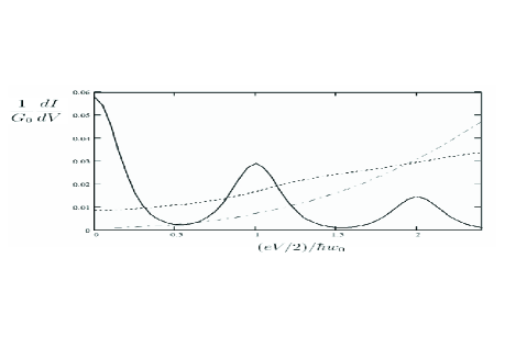
Figure 3: Differential conductance (in the units of $G_{0}$) as a function of driving voltage (in the units of $\hbar w_{0}$) for the case $g<1/2$. Here $\Gamma/kT=0.01$; $\hbar w_{0}/kT$; $\lambda^{2}$; and $\varepsilon_{0}$ are the same as on Fig.2. Solid line corresponds to the case of noninteracting leads: $g=1$; dot line corresponds to value $g=0.45$; dash-dot line - to $g=0.25$. One can see from the figure that for $g<1/2$ the resonance-like behavior of differential conductance disappears and conductance scales as a power-law of the bias voltage.

The resonant behavior disappears for strong interaction $g<1/2$ (Figs.2,3), when at low temperatures $T\ll\hbar w_{0}$ differential conductance scales with bias voltage as $G(V)\propto V^{1/g-2}$ in accordance with the Luttinger liquid prediction for nonlinear electron transport through a single-level quantum dot. For instance, if we put $1/g=n,\,(n=2,3,\ldots)$ and tune the level energy to the resonance point $\varepsilon_{0}=\lambda^{2}\hbar w_{0}$ -(”resonant” location of the level in the presence of ”polaronic” shift), we obtain for the differential conductance $G(V)$ the following expression for $eV/\hbar w_{0}\gg(1/g-2)$

$$G(V)\simeq 4\pi G_{0}\frac{\Gamma_{\lambda}}{\Lambda}\cdot\left[\frac{1}{(n-1)!}\right]\cdot\left(\frac{eV}{2\Lambda}\right)^{n-2}\ ,$$ (22)

where $\Gamma_{\lambda}=\Gamma\exp(-\lambda^{2})$. One can readily see that expression (22) reproduces Furusaki temperature scaling Eq.(19) when $eV$ is replaced by $T$.

Analogous interplay of Kane-Fisher and polaronic effects one can see on Figs.4,5, where differential conductance is plotted as a function of level energy $\varepsilon_{0}$ (or, equivalently, as a function of gate voltage). For noninteracting leads $(g=1)$ the resonance conductance peaks correspond to the level positions at $\varepsilon_{P\pm}=\varepsilon_{F}\pm eV/2$ (in our plot we put: $eV=5\hbar w_{0}$). This elastic resonance peak is suppressed by electron-electron interaction in the leads $(g<1)$. The dependence $G(V_{g})$ for weak and moderately strong interaction still reveals resonance structure with 4 satellites in our case (see Fig.4). The inelastic resonance peaks disappear at $g<1/2$ and maximum of differential conductance corresponds at $g\ll 1$ to the level position at $\varepsilon_{P}(V_{g})=\varepsilon_{F}$, that is exactly in the middle between chemical potentials of left and right electrodes (see Fig.5).

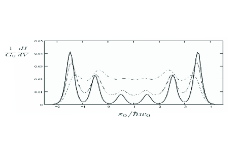
Figure 4: Differential conductance (in the units of $G_{0}$) as a function of level energy $\varepsilon_{0}$, counted from the Fermi energy for the case $g>1/2$. Solid line corresponds to the case of noninteracting leads: $g=1$; dot line corresponds to value $g=0.8$; dash-dot line - to $g=0.6$. The bias voltage $eV/\hbar\omega_{0}=5$ is sufficiently high to excite vibrons and to support electron transport through inelastic channels. All parameters are the same as for Fig.2.

Figure 5: Differential conductance (in the units of $G_{0}$) as a function of level energy $\varepsilon_{0}$, counted from the Fermi energy for the case $g<1/2$. Solid line corresponds to the case of noninteracting leads: $g=1$; dot line corresponds to value $g=0.45$; dash-dot line - to $g=0.25$. The bias voltage $eV/\hbar\omega_{0}=5$ is sufficiently high to excite vibrons and to support electron transport through inelastic channels. All parameters are the same as for Fig.3.

It is important to stress here once more that for moderately strong electron-electron interaction in the leads the inelastic tunnelling can dominate in electron transport. One can see from Figs.2-5 that there is region of coupling constants when the first satellite peak is higher than the ”main” (zero-bias) resonant peak, which corresponds to elastic ($l=0$) tunnelling channel. It is the most significant prediction, we have made in this paper.

IV The noise power

The knowledge of tunnelling rates Eqs.(8,9) allows us to evaluate not only the average current Eq.(6) but the noise power as well. We will follow the method developed in Refs. 21 ; 22 where quantum noise was calculated for resonant electron transport through a quantum dot weakly coupled to noninteracting electrodes.

The noise power is defined (see e.g. 23 ) as

$$S(w)=2\int_{-\infty}^{\infty}dt\exp(iwt)\langle\Delta I(t)\Delta I(0)\rangle\ ,$$ (23)

where $\Delta I(t)=I(t)-I$ ($I$ is the average current). The noise defined in Eq.(23), in the case of sequential tunnelling through a quantum dot, can be expressed in terms of tunnelling rates. For a single level quantum dot this formula for low frequency noise $S=S(w=0)$ takes the form

$$S=2eI-\frac{4I^{2}}{\Gamma_{\Sigma}}+4e^{2}\frac{\Gamma_{01}^{L}\Gamma_{10}^{R}}{\Gamma_{\Sigma}}\ ,$$ (24)

here the average current $I$ is determined by Eq.(6). The noise power Eq.(24) depends on temperature and bias voltage $S(T,V)$ and contains both thermal (Jonson-Nyquist) noise $S_{JN}(T)\equiv S(T,V=0)=4TG(T)$ ($G$ is the conductance) and the non-equilibrium (shot) noise $S_{sh}(T,V)$. Since the thermal noise is totally determined by temperature dependence of conductance, we will study in what follows only shot noise and Fano factor $F=S_{sh}/2eI$. In particular, Fano factor in our case can be represented as follows

$$F=\left\{1-\frac{2I}{e\Gamma_{\Sigma}}+\frac{2e}{I}\left(\frac{\Gamma_{01}^{L}\Gamma_{10}^{R}}{\Gamma_{\Sigma}}-\frac{TG}{e^{2}}\right)\right\}\ .$$ (25)

For noninteracting leads $(g=1)$ and noninteracting quantum dot $(\lambda=0)$ one readily gets from Eqs.(13),(24) a simple expression for the ”full” noise $(S)$ of a single electron transistor (SET). On resonance $\varepsilon_{P}(V_{g})=\varepsilon_{F}$ and at temperatures $T\gg\Gamma$ one finds

$$S=\frac{2e^{2}\Gamma}{\hbar}\tanh\left(\frac{eV}{4T}\right)\left[1-\frac{2\Gamma}{\Gamma_{\Sigma}}\tanh\left(\frac{eV}{4T}\right)\right]$$

$$+\frac{e^{2}\Gamma}{\hbar}\left[\frac{\exp(-eV/4T)}{\cosh^{2}(eV/4T)}\right]\ .$$ (26)

From Eq.(26) in the limit $V\rightarrow 0$ we obtain $S=S_{JN}(T)$, where $S_{JN}(T)=e^{2}\Gamma/\hbar=4TG$ is the thermal noise. In the opposite case $eV\gg T$ we rederive the well-known formulae for the shot-noise and the Fano factor of a single level quantum dot 21 ; 22 ; 23

$$S_{sh}=\frac{2e^{2}\Gamma}{\hbar}\left(1-\frac{2\Gamma}{\Gamma_{\Sigma}}\right)\,\,,\,\,F=1-\frac{2\Gamma}{\Gamma_{\Sigma}}\ .$$ (27)

These formulae (26),(27) can be also re-derived from the general expression for the full noise of noninteracting electrons (see e.g., Eq.(61) in Ref.23 )

$$S(V,T)=\frac{e^{2}}{\hbar}\int d\varepsilon T_{t}(\varepsilon)[f_{L}(1-f_{L})+f_{R}(1-f_{R})]$$

$$+\frac{e^{2}}{\hbar}\int d\varepsilon T_{t}(\varepsilon)\left[1-T_{t}(\varepsilon)\right](f_{L}-f_{R})^{2}\ ,$$ (28)

where $T_{t}(\varepsilon)$ is the transmission coefficient and $f_{j}=\left\{\exp\left[(\varepsilon-\mu_{j})/T\right]+1\right\}^{-1}$ is the equilibrium distribution function of electrons in the leads ($\mu_{j}$ is the chemical potential; $j=L,R$). In the case of single level quantum dot $T_{t}(\varepsilon)$ takes the form Breit-Wigner tunnelling probability

$$T_{t}(\varepsilon)=\frac{\Gamma_{L}\Gamma_{R}}{\left(\varepsilon-\varepsilon_{P}\right)^{2}+(\Gamma_{L}+\Gamma_{R})^{2}/4}\,$$ (29)

where $\Gamma\equiv\Gamma_{L}\Gamma_{R}/\left(\Gamma_{L}+\Gamma_{R}\right)$. For a weak tunnelling when $\Gamma_{L(R)}$ are the smallest energy scales in the problem the Lorentzian shape of the Breit-Wigner resonance shrinks to $\delta$-function

$$T_{t}(\varepsilon)|_{\Gamma_{L,R}\rightarrow 0}\simeq 2\pi\Gamma\delta(\varepsilon-\varepsilon_{P})\ .$$ (30)

With the help of Eqs.(28),(30) for the resonance condition $\varepsilon_{P}(V_{g})=\varepsilon_{F}$ we easily re-derive Eqs.(26). (Notice, that in sequential tunnelling approach the tunnelling transitions through the left and right barriers are assumed to be weak and uncorrelated. Therefore we can safely neglect $T_{t}^{2}$-term in Eq.(28)). It is evident from Eqs.(25),(27) that for noninteracting electrons the Fano factor is sub-Poissonian $(F\leq 1)$ and $F$ approaches $1$ for strongly asymmetric junction $\Gamma_{L(R)}\gg\Gamma_{R(L)}$ and for $eV\gg T$.

The master equation approach we have used in our analysis holds when electron tunnelling amplitudes are small. For noninteracting electrons this assumption is satisfied when electron energies are far from the resonant energy level, i.e. $T_{t}(\varepsilon)\ll 1$. The differential shot noise in this case as a function of bias voltage or gate voltage behaves similarly to the differential conductance. Notice however that due to different dependence on temperature the shot noise unlike the thermal one even in sequential tunnelling regime ($T\gg\Gamma$) can not be expressed in terms of conductance.

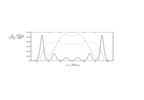
Figure 6: Differential shot noise power (in the units of $eG_{0}$) as function of the level energy $\varepsilon_{0}$ in the nonlinear transport regime (when $eV/\hbar\omega_{0}=5$) for the case $g<1/2$. Solid line corresponds to the case of noninteracting leads $g=1$; dot line corresponds to value $g=0.45$; dash-dot line - to $g=0.25$. Other parameters are the same as on Fig.5.

Figure 7: Fano factor for the case $g<1/2$ as the function of the level energy $\varepsilon_{0}$ in the nonlinear transport regime (when $eV/\hbar\omega_{0}=5$) which corresponds to Figs.5,6. Solid line corresponds to the case of noninteracting leads $g=1$; dot line corresponds to value $g=0.45$; dash-dot line - to $g=0.25$. All other parameters are the same as on Figs.5,6.

By comparing Fig.6 with Fig.5, one can see that the above similarity is preserved for interacting electrons ($g\neq 1,\,\lambda\neq 0$) as well. The corresponding Fano factor which is the ”shot noise/current” ratio and thus is less sensitive to the details of tunnelling process, for strong electron-electron interaction exhibits a simple behavior (see Fig.7). It dips ($F\simeq 1/2$) at symmetric (with respect to chemical potentials of the leads) position of the dot level. Outside this region $F\rightarrow 1$ (Poissonian noise). The width of the dip decreases with the increase of interaction (see Fig.7).

V Summary

We considered the influence of interaction on transport properties of molecular transistor which was modelled as a vibrating single-level quantum dot weakly coupled to the Luttinger liquid leads. We found interesting interplay between polaronic and Luttinger liquid effects in our system. In particular it was shown that for weak or moderately strong interaction ($1/2<g\leq 1$) the differential conductance demonstrates resonance-like behavior and for moderately strong interaction inelastic channels can even dominate in electron transport through a vibrating quantum dot. For strong interaction ($g\ll 1$) the resonant character of vibron-assisted tunnelling disappears and the differential conductance scales as a power law on temperature (linear regime $T\gg eV$) or on bias voltage (nonlinear regime $eV\gg T$).

The authors would like to thank S.I.Kulinich for valuable discussions. This work was partly supported by the joint grant of the Ministries of Education and Science in Ukraine and Israel and by the grant ”Effects of electronic, magnetic and elastic properties in strongly inhomogeneous nanostructures” of the National Academy of Sciences of Ukraine.

References

- (1) A.Nitzan and M.A.Ratner, Science 300, 1384 (2003).
- (2) M.Galperin, M.A.Ratner, A.Nitzan, J.Phys.:Cond.Matt. 19, 103201 (2007).
- (3) R.I.Shekhter, Zh.Eksp.Teor.Fiz. 68, 623 (1975).
- (4) I.O.Kulik and R.I.Shekhter, Zh.Eksp.Teor.Fiz. 63, 1400 (1972).
- (5) Single Charge Tunneling, edited by H.Grabert and M.H.Devoret, NATO ASI Ser.B, vol.294, Plenum Press, N.Y., (1992).
- (6) L.I.Glazman, R.I.Shekhter,Zh.Eksp.Teor.Fiz. 94, 292 (1988) [Sov.Phys.JETP 67, 163 (1988)].
- (7) S.Braig, K.Flensberg, Phys.Rev.B 68, 205324 (2003).
- (8) L.Y.Gorelik, A.Isacsson, M.V.Voinova, B.Kasemo, R.I.Shekhter, M.Jonson, Phys.Rev.Lett. 80, 4526 (1998).
- (9) R.I.Shekhter, L.Y.Gorelik, M.Jonson, Y.M.Galperin, V.M.Vinokur, J.Comput.Theor.Nanosci. 4, 860 (2007).
- (10) U.Lundin, R.M.McKenzie, Phys.Rev.B 66, 075303 (2002).
- (11) J.Koch, F. von Oppen, A.V.Andreev, Phys.Rev.B, 74, 205438 (2006).
- (12) H.Park, J.Park, A.K.L.Lim, E.H.Anderson, A.P.Alivisatos, P.L.McEuen, Nature 407, 57 (2000).
- (13) H.W.Ch.Postma,T.Teepen, Z.Yao, M.Grifoni, C.Dekker, Science 239, 76 (2001).
- (14) A.Furusaki, Phys.Rev.B 57, 7141 (1998).
- (15) C.L.Kane, M.P.A.Fisher, Phys.Rev.B 46, 15233 (1992).
- (16) Yu.V.Nazarov and L.I.Glazman, Phys.Rev.Lett. 91, 126804 (2003).
- (17) G.D.Mahan, Many-Particle Physics, Plenum Press, New York (1990).
- (18) A.Komnik and A.O.Gogolin, Phys.Rev.Lett. 90, 246403 (2003).
- (19) ”I.S.Gradshtein, and I.M.Ryzhik, Tables of Integrals, Series and Products, Academic Press, NY (1965).
- (20) I.V.Krive, R.Ferone, R.I.Shekhter, M.Jonson, P.Utko, J.Nygard, New J.Phys., (2008) to be published.
- (21) S.Hershfield, J.H.Davies, P.Hyldgaard, C.J.Stanton, J.W.Wilkins, Phys.Rev.B 47, 1967 (1993).
- (22) I.Djuric, B.Dong, H.L.Cui, J.Appl.Phys. 99, 063710 (2006).
- (23) Y.M.Blanter, M.Buttiker, Shot Noise in Mesoscopic Conductors, Phys.Rep. 336, pp.1-166, (2000).