On the anomalous enhancement observed in $B\to D^{(*)}\,\tau\,{\bar{\nu}}_{\tau}$ decays

Abstract

The BaBar measurements of the ratios ${\cal R}(D^{(*)})=\frac{{\cal B}(B\to D^{(*)}\tau{\bar{\nu}}_{\tau})}{{\cal B}(B\to D^{(*)}\mu{\bar{\nu}}_{\mu})}$ deviate from the standard model expectation, while new results on the purely leptonic $B\to\tau{\bar{\nu}}_{\tau}$ mode show a better consistency with the standard model, within the uncertainties. In a new physics scenario, one possibility to accomodate these two experimental facts consists in considering an additional tensor operator in the effective weak hamiltonian. We study the effects of such an operator in a set of observables, in semileptonic $B\to D^{(*)}$ modes as well as in semileptonic $B$ and $B_{s}$ decays to excited positive parity charmed mesons.

I Introduction

The BaBar measurements of the rates of $B^{-}$ and ${\bar{B}}^{0}$ semileptonic decays into $D^{(*)}$ and a $\tau$ lepton seem to indicate a significant deviation from the standard model (SM) expectation. The experimental results concern the $B\to D^{(*)}\tau{\bar{\nu}}_{\tau}$ decay widths normalized to the widths of the corresponding modes having a light $\ell=e,\,\mu$ lepton in the final state Lees:2012xj :

$${\cal R}^{-}(D)=\frac{{\cal B}(B^{-}\to D^{0}\tau^{-}\,{\bar{\nu}}_{\tau})}{{\cal B}(B^{-}\to D^{0}\ell^{-}\,{\bar{\nu}}_{\ell})}=0.429\pm 0.082\pm 0.052\,\,\,, {\cal R}^{-}(D^{*})=\frac{{\cal B}(B^{-}\to D^{*0}\tau^{-}\,{\bar{\nu}}_{\tau})}{{\cal B}(B^{-}\to D^{*0}\ell^{-}\,{\bar{\nu}}_{\ell})}=0.322\pm 0.032\pm 0.022\,\,,$$

$${\cal R}^{0}(D)=\frac{{\cal B}({\bar{B}}^{0}\to D^{+}\tau^{-}\,{\bar{\nu}}_{\tau})}{{\cal B}({\bar{B}}^{0}\to D^{+}\ell^{-}\,{\bar{\nu}}_{\ell})}=0.469\pm 0.084\pm 0.053\,\,\,, {\cal R}^{0}(D^{*})=\frac{{\cal B}({\bar{B}}^{0}\to D^{*+}\tau^{-}\,{\bar{\nu}}_{\tau})}{{\cal B}({\bar{B}}^{0}\to D^{*+}\ell^{-}\,{\bar{\nu}}_{\ell})}=0.355\pm 0.039\pm 0.021\,\,$$

(the first and second error are the statistic and systematic uncertainty, respectively). The measurements have been estimated to deviate at the global level of 3.4$\sigma$ with respect to SM predictions Lees:2012xj ; Fajfer:2012vx . Therefore, there is the possibility that semileptonic processes involving heavy quarks and the $\tau$ lepton are unveiling the effects of particles with large couplings to the heavier fermions, as it is natural for charged scalars which could contribute to the tree-level $b\to c\ell\bar{\nu}$ transitions Fajfer:2012vx ; Fajfer:2012jt ; Becirevic:2012jf ; Datta:2012qk ; Celis:2012dk ; Crivellin:2012ye ; Choudhury:2012hn ; Tanaka:2012nw .

Before the observation of these possible hints of new physics (NP) in semileptonic $b\to c$ decays, the first experimental analyses of the purely leptonic $B^{-}\to\tau^{-}{\bar{\nu}}_{\tau}$ mode also reported an excess of events. In SM the ${\cal B}(B^{-}\to\tau^{-}{\bar{\nu}}_{\tau})$ branching fraction is given by

$${\cal B}(B^{-}\to\tau^{-}{\bar{\nu}}_{\tau})={G_{F}^{2}m_{B}m_{\tau}^{2}\over 8\pi}\left(1-{m_{\tau}^{2}\over m_{B}^{2}}\right)^{2}f_{B}^{2}\,|V_{ub}|^{2}\,\tau_{B^{-}}\,\,,$$ (2)

neglecting a tiny electromagnetic radiative correction. Using the lattice QCD average for the $B$ decay constant $f_{B}=(190.6\pm 4.7)$ MeV quoted in Laiho:2009eu , and varying the Cabibbo-Kobayashi-Maskawa (CKM) matrix element $|V_{ub}|$ in the range determined from inclusive and exclusive $B$ decays: $|V_{ub}|=0.0035\pm 0.0005$, the prediction follows: ${\cal B}(B^{-}\to\tau^{-}{\bar{\nu}}_{\tau})=(0.79\pm 0.23)\times 10^{-4}$, in agreement with the outcome of CKM matrix fits Bona:2009cj ; Lenz:2010gu . This value is smaller by about a factor of 2 than the experimental results reported in Ikado:2006un ; Hara:2010dk ; Aubert:2007xj ; Aubert:2009wt and compiled in Rosner:2012np : ${\cal B}(B^{-}\to\tau^{-}{\bar{\nu}}_{\tau})=(1.68\pm 0.31)\times 10^{-4}$. However, new Belle Adachi:2012mm and BaBar Lees:2012ju measurements, obtained using the hadronic tagging method,

$${\cal B}(B^{-}\to\tau^{-}{\bar{\nu}}_{\tau}) = \left(0.72^{+0.27}_{-0.25}\pm 0.11\right)\times 10^{-4}\,\,\,\,\,{\rm(Belle)}$$

$${\cal B}(B^{-}\to\tau^{-}{\bar{\nu}}_{\tau}) = \left(1.83^{+0.53}_{-0.49}\pm 0.24\right)\times 10^{-4}\,\,\,\,\,{\rm(BaBar)}$$ (3)

are more consistent with SM, and draw the average ${\cal B}(B^{-}\to\tau^{-}{\bar{\nu}}_{\tau})$ to a smaller value: ${\cal B}(B^{-}\to\tau^{-}{\bar{\nu}}_{\tau})=(1.12\pm 0.22)\times 10^{-4}$, after the combination with the semileptonic tagging method results, see fig.1.

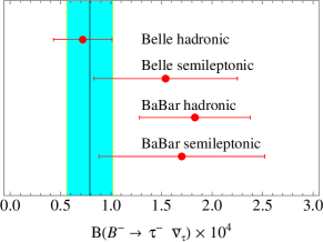
Figure 1: Experimental results for ${\cal B}(B^{-}\to\tau^{-}{\bar{\nu}}_{\tau})$ Aubert:2009wt ; Hara:2010dk ; Adachi:2012mm ; Lees:2012ju together with the SM expectation corresponding to $|V_{ub}|=0.0035\pm 0.0005$ (vertical band).

The different trend of the measurements involving $\tau$ in $B$ leptonic and semileptonic decay modes poses two questions. The first one concerns the level of accuracy of the SM predictions for the ratios in (LABEL:data). The second one is which kind of new physics effects, if any, could modify the ratios (LABEL:data) without affecting the purely leptonic mode. Indeed, several analyses devoted to try to explain the anomalies in $B\to D^{(*)}\tau{\bar{\nu}}_{\tau}$ within new physics scenarios have considered as possible candidates models with new scalars having couplings to leptons proportional to the lepton mass, to guarantee the enhancement of the $\tau$ modes. This is the case of models with two Higgs doublets (2HDM), the best known example being the minimal supersymmetric standard model in which two Higgs doublets are required to give mass to down-type quarks and charged leptons in one case, and up-type quarks in the other. In this framework, the ratios (LABEL:data) depend on the mass of the charged Higgs $H^{\pm}$ and the ratio $\beta$ of the two Higgs doublet VEVs, and no choice of such parameters allows to simultaneously reproduce the experimental data on ${\cal R}(D)$ and ${\cal R}(D^{*})$ Lees:2012xj . Variants of the 2HDM Crivellin:2012ye ; Celis:2012dk , together with other models providing explicit flavour violation Fajfer:2012jt , might explain the measurements (LABEL:data); however, an enhancement of the purely leptonic $B$ decay rate is generally implied.

In this paper we reconsider both the above mentioned issues. We reanalyse the SM prediction for $B\to D^{(*)}\ell{\bar{\nu}}_{\ell}$, specifying the main sources of uncertainties and possible improvements. Our results confirm that the most significant deviation is for ${\cal R}(D^{*})$. Then, we scrutinize the effects of possible NP contributions in the effective weak Hamiltonian having a structure able to affect the ratios (LABEL:data) but leaving the pure $B$ leptonic modes unchanged. In particular, we focus on a NP operator constructed from tensor quark and lepton currents. Such a kind of operators have been also investigated in Becirevic:2012jf and Tanaka:2012nw , but we devote the main attention to differential distributions, namely the lepton forward-backward differential asymmetries, in which the sensitivity to the new Dirac structure is maximal, as emphasized in Datta:2012qk for different operators. Although there are scenarios in which tensor operators are generated, in our analysis we do not rely on explicit models: our purpose is to identify physical observables having a mild sensitivity to hadronic uncertainties, which therefore can be used to unveil effects easier to interpret. It is only worth mentioning that these operators emerge, for example, in models with new coloured bosons carrying both lepton and baryon quantum number (referred to as leptoquarks, LQ): SU(5)_GUT Georgi:1974sy , Pati-Salam SU(4) Pati:1974yy , composite Schrempp:1984nj , superstrings Hewett:1988xc and technicolor models Dimopoulos:1979es . In the most general formulation of these models scalar operators may also occur. Leptoquarks couple to quarks and leptons and, from limits on flavour changing neutral currents, preferably to those within the same SM generation. Searches for leptoquarks decaying to 2$\tau$ and 2$b$ jets, performed by the CMS Collaboration at the CERN LHC, bound (preliminarly) the mass of a possible scalar leptoquark to $M(LQ)>525$ GeV, and to $M(LQ)>760$ GeV for a vector leptoquark cms ; other bounds can be found in leptoquarks .

In our analysis of semileptonic $B$ decays, we first consider $D$ and $D^{*}$ mesons in the final state, and then turn to the interesting case of final states with excited positive parity charmed mesons.

II Exclusive $b\to c\ell{\bar{\nu}}_{\ell}$ Decays

We consider the $b\to c\ell{\bar{\nu}}_{\ell}$ effective hamiltonian comprising the SM term and an additional operator Becirevic:2012jf ; Tanaka:2012nw :

$$H_{eff}=H_{eff}^{SM}+H_{eff}^{NP}={G_{F}\over\sqrt{2}}V_{cb}\left[{\bar{c}}\gamma_{\mu}(1-\gamma_{5})b\,{\bar{\ell}}\gamma^{\mu}(1-\gamma_{5}){\bar{\nu}}_{\ell}+\epsilon_{T}^{\ell}\,{\bar{c}}\sigma_{\mu\nu}(1-\gamma_{5})b\,{\bar{\ell}}\sigma^{\mu\nu}(1-\gamma_{5}){\bar{\nu}}_{\ell}\right]\,\,\,.$$ (4)

$G_{F}$ is the Fermi constant and $V_{cb}$ the CKM matrix element. $\epsilon_{T}^{\ell}$ is the relative complex coupling of the new tensor term with respect to the SM one. It is assumed that the main coupling is to the heaviest lepton, hence we set $\epsilon_{T}^{\ell}=0$ for $\ell=e,\mu$ and $\epsilon_{T}\equiv\epsilon_{T}^{\tau}$. This coupling can be bound experimentally, so that the effects of the new operator can be scrutinized in physical observables which, in general, are expressed as a SM, a new physics and an interference contribution. For example, the differential $B(p)\to M_{c}(p^{\prime})\ell(p_{1}){\bar{\nu}}_{\ell}(p_{2})$ decay rate, with $M_{c}$ a charmed meson, reads:

$${d\Gamma\over dq^{2}}(B\to M_{c}\ell\bar{\nu}_{\ell})=C(q^{2})\left[{d\tilde{\Gamma}\over dq^{2}}(B\to M_{c}\ell\bar{\nu}_{\ell})\Big{|}_{SM}+{d\tilde{\Gamma}\over dq^{2}}(B\to M_{c}\ell\bar{\nu}_{\ell})\Big{|}_{NP}+{d\tilde{\Gamma}\over dq^{2}}(B\to M_{c}\ell\bar{\nu}_{\ell})\Big{|}_{INT}\right]\,,$$ (5)

with $q=p-p^{\prime}$ and $C(q^{2})$ defined as

$$C(q^{2})={G_{F}^{2}|V_{cb}|^{2}\lambda^{1/2}(m_{B}^{2},m_{M_{c}}^{2},q^{2})\over 192\pi^{3}m_{B}^{3}}\left(1-{m_{\ell}^{2}\over q^{2}}\right)^{2}\,\,\,;$$ (6)

$\lambda(x,y,z)=x^{2}+y^{2}+z^{2}-2(xy+xz+yz)$ is the triangular function. To compute the three terms in (5) we need the relevant hadronic matrix elements.

II.1 $B\to D\ell{\bar{\nu}}_{\ell}$

The hadronic matrix elements in $B\to D\ell{\bar{\nu}}_{\ell}$ can be parametrized in a standard way,

$$<D(p^{\prime})|{\bar{c}}\gamma_{\mu}b|B(p)> = F_{1}(q^{2})(p+p^{\prime})_{\mu}+{m_{B}^{2}-m_{D}^{2}\over q^{2}}\left[F_{0}(q^{2})-F_{1}(q^{2})\right]q_{\mu}\,\,\,,$$ (7)

$$<D(p^{\prime})|{\bar{c}}\sigma_{\mu\nu}(1-\gamma_{5})b|B(p)> = {F_{T}(q^{2})\over m_{B}+m_{D}}\,\epsilon_{\mu\nu\alpha\beta}p^{\prime\alpha}p^{\beta}+i\,{G_{T}(q^{2})\over m_{B}+m_{D}}\,(p_{\mu}p^{\prime}_{\nu}-p_{\nu}p^{\prime}_{\mu})\,,$$ (8)

(with $F_{T}=G_{T}$ from the relation $\sigma_{\mu\nu}\gamma_{5}=\frac{i}{2}\epsilon_{\mu\nu\alpha\beta}\,\sigma^{\alpha\beta}$), so that the three terms in (5) read:

$${d\tilde{\Gamma}\over dq^{2}}(B\to D\ell\bar{\nu}_{\ell})\Big{|}_{SM} = \lambda(m_{B}^{2},m_{D}^{2},q^{2})\left(1+{m_{\ell}^{2}\over 2q^{2}}\right)\left[F_{1}(q^{2})\right]^{2}+m_{B}^{4}\left(1-{m_{D}^{2}\over m_{B}^{2}}\right)^{2}{3m_{\ell}^{2}\over 2q^{2}}\left[F_{0}(q^{2})\right]^{2}\,,$$ (9)

$${d\tilde{\Gamma}\over dq^{2}}(B\to D\ell\bar{\nu}_{\ell})\Big{|}_{NP} = {|\epsilon_{T}|^{2}\over 2}{q^{2}\over(m_{B}+m_{D})^{2}}\,\lambda(m_{B}^{2},m_{D}^{2},q^{2})\left(1+2{m_{\ell}^{2}\over q^{2}}\right)\,\left[F_{T}(q^{2})+G_{T}(q^{2})\right]^{2}\,,$$ (10)

$${d\tilde{\Gamma}\over dq^{2}}(B\to D\ell\bar{\nu}_{\ell})\Big{|}_{INT} = -3Re[\epsilon_{T}]{m_{\ell}\over m_{B}+m_{D}}\,\lambda(m_{B}^{2},m_{D}^{2},q^{2})\,F_{1}(q^{2})\,\left[F_{T}(q^{2})+G_{T}(q^{2})\right]\,.$$ (11)

In the infinite heavy quark mass limit, formalized by the heavy quark effective theory (HQET), the form factors in (7-8) can all be related to the Isgur-Wise function $\xi$ Isgur:1989ed . The result is known hqet ; hqet1 : expressing $F_{1}(q^{2})$ and $F_{0}(q^{2})$ in terms of two other form factors $h_{+}(w)$ and $h_{-}(w)$:

$$F_{1}(q^{2}) = \frac{1}{2\sqrt{m_{B}m_{D}}}\left[(m_{B}+m_{D})h_{+}(w)-(m_{B}-m_{D})h_{-}(w)\right]$$ (12)

$$\frac{m_{B}^{2}-m_{D}^{2}}{q^{2}}\left[F_{0}(q^{2})-F_{1}(q^{2})\right] = \frac{1}{2\sqrt{m_{B}m_{D}}}\left[(m_{B}+m_{D})h_{-}(w)-(m_{B}-m_{D})h_{+}(w)\right]\,\,,$$ (13)

and defining the meson momenta in terms of four-velocities, $p=m_{B}v$ and $p^{\prime}=m_{D}v^{\prime}$, with $w=v\cdot v^{\prime}$ and $q^{2}=m_{B}^{2}+m_{D}^{2}-2m_{B}m_{D}w$, at the leading order in the heavy quark and $\alpha_{s}$ expansion one has

$$h_{+}(w)=\xi(w)\,\,\,\,,\hskip 28.45274pth_{-}(w)=0\,\,\,,$$ (14)

with $\xi(w)$ the Isgur-Wise function. Also the form factors in (8) are related to $\xi(w)$ at the same order expansion:

$$F_{T}(q^{2})=G_{T}(q^{2})={m_{B}+m_{D}\over\sqrt{m_{B}m_{D}}}\,\xi(w)\,\,\,.$$ (15)

At the next-to-leading order, corrections must be taken into account, which at first are needed for the study of the decay in SM. We elaborate a determination of the functions $h_{+}$, $h_{-}$ and $\xi$ based on a combination of experimental and theoretical information. The experimental input comes from the BaBar analysis of $B\to D\mu{\bar{\nu}}_{\mu}$ Aubert:2009ac , the differential rate of which, neglecting the lepton mass, reads:

$${d\Gamma\over dw}(B\to D\ell\bar{\nu}_{\ell})={G_{F}^{2}|V_{cb}|^{2}\over 48\pi^{3}}m_{B}^{5}r^{3}(1+r)^{2}(w^{2}-1)^{3/2}[F_{D}(w)]^{2}\,\,\,,$$ (16)

with

$$F_{D}(w)=\left[h_{+}(w)-{1-r\over 1+r}h_{-}(w)\right]$$ (17)

and $\displaystyle r=\frac{m_{D}}{m_{B}}$. Using the parametrization Caprini:1997mu

$$F_{D}(w)=F_{D}(1)\Big{\{}1-8\rho_{1}^{2}z+(51\rho_{1}^{2}-10)z^{2}-(252\rho_{1}^{2}-84)z^{3}\Big{\}}\,\,\,$$ (18)

in terms of the variable

$$z={\sqrt{w+1}-\sqrt{2}\over\sqrt{w+1}+\sqrt{2}}\,\,\,,$$ (19)

from the fit of the product $G^{BaBar}(w)=F_{D}(w)|V_{cb}|$ the BaBar Collaboration provides the parameters $G^{BaBar}(1)=F_{D}(1)|V_{cb}|$ and $\rho_{1}^{2}$. The outcome of the fit is slightly different for $B^{-}$ or ${\bar{B}}^{0}$ modes; we consider for definiteness the ${\bar{B}}^{0}$ case Aubert:2009ac ,

$$G^{BaBar}(1)=(44.9\pm 3.2\pm 1.6)\,10^{-3}\,\,\,,\hskip 28.45274pt\rho_{1}^{2}=1.29\pm 0.14\pm 0.05\,\,.$$ (20)

This result can be translated into a determination of $\xi(w)$, expressing the form factors $h_{\pm}(w)$ in terms of the Isgur-Wise function and including the $\alpha_{s}$ and $1/m_{b,c}$ corrections worked out by M. Neubert in hqet and by I. Caprini et al., in Caprini:1997mu :

$$h_{+}(w) = \left[C_{1}+{w+1\over 2}(C_{2}+C_{3})+(\epsilon_{b}+\epsilon_{c})L_{1}\right]\xi(w)={\tilde{h}}_{+}(w)\,\xi(w)$$ (21)

$$h_{-}(w) = \left[{w+1\over 2}(C_{2}-C_{3})+(\epsilon_{c}-\epsilon_{b})L_{4}\right]\xi(w)={\tilde{h}}_{-}(w)\,\xi(w)$$ (22)

with $\epsilon_{b}=\displaystyle{1\over 2m_{b}}$, $\epsilon_{c}=\displaystyle{1\over 2m_{c}}$. The coefficients $C_{1,2,3}$ and $L_{i}$ are collected in appendix A. $C_{i}$ account for the perturbative corrections, $L_{i}$ for the heavy quark mass corrections and depend on the hadronic parameter $\bar{\Lambda}$, the difference between the heavy meson ($B,\,D$) and the heavy quark ($b,\,c$) mass in the heavy quark limit. We use $m_{b}=4.8$ GeV and $m_{c}=1.4$ GeV and a conservative value ${\bar{\Lambda}}=0.5\pm 0.2$ GeV hqet , so that the uncertainty in ${\bar{\Lambda}}$ encompasses the error on ${\bar{\Lambda}}/m_{b}$ and ${\bar{\Lambda}}/m_{c}$. The Isgur-Wise function $\xi(w)$ resulting from

$$|V_{cb}|\,\xi(w)=\frac{G^{BaBar}(w)}{\left[\tilde{h}_{+}(w)-{1-r\over 1+r}\,\tilde{h}_{-}(w)\right]}\,\,$$ (23)

is depicted in fig.2 (left panel).

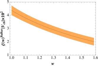
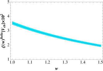
Figure 2: Isgur-Wise function $\xi(w)$ (times $|V_{cb}|\times 10^{2}$) obtained using the BaBar data on ${\bar{B}}^{0}\to D^{+}\ell^{-}\bar{\nu}_{\ell}$ (left) and the Belle data on ${\bar{B}}^{0}\to D^{*+}\ell^{-}\bar{\nu}_{\ell}$ (right) . The width of the curves is due to the errors in the parameters fitted in the two cases and to the uncertainty on ${\bar{\Lambda}}$ and $\alpha_{s}$ in the determination of the form factor.

The form factors needed for analysis of the mode with $\tau$ can be separately derived using again Eqs.(21,22):

$$|V_{cb}|\,h_{+}(w) = \frac{1}{1-{1-r\over 1+r}\,A(w)}\,\,G^{BaBar}(w)$$ (24)

$$|V_{cb}|\,h_{-}(w) = \frac{A(w)}{1-{1-r\over 1+r}\,A(w)}\,\,G^{BaBar}(w)$$ (25)

with $A=\tilde{h}_{-}/\tilde{h}_{+}$. For the matrix elements of the tensor operator, we use $\xi(w)$ also in (15). In the standard model, the results for the semileptonic ${\bar{B}}^{0}\to D^{+}$ branching fractions can be quoted as

$${\cal B}({\bar{B}}^{0}\to D^{+}\ell^{-}{\bar{\nu}}_{\ell})\Big{|}_{SM} = (2.15\pm 0.45)\times 10^{-2}$$ (26)

$${\cal B}({\bar{B}}^{0}\to D^{+}\tau^{-}{\bar{\nu}}_{\tau})\Big{|}_{SM} = (0.70\pm 0.12)\times 10^{-2}$$ (27)

and, taking the correlation between the predictions for $\ell$ and $\tau$ into account,

$${\cal R}^{0}(D)\Big{|}_{SM}=\frac{{\cal B}({\bar{B}}^{0}\to D^{+}\tau^{-}{\bar{\nu}}_{\tau})}{{\cal B}({\bar{B}}^{0}\to D^{+}\ell^{-}{\bar{\nu}}_{\ell})}\Big{|}_{SM}=0.324\pm 0.022\,\,\,.$$ (28)

The SM prediction for ${\cal R}^{0}(D)$ deviates from the measurement (LABEL:data) (with statistic and systematic uncertainties combined in quadrature) by about 1.5$\sigma$ . The deviation is smaller in the charged ${\cal R}^{-}(D)$ case.

The stability of (28) against changes of the input information on form factors is noticeable: sensitivity to $1/m_{Q}$ corrections can be estimated varying $\bar{\Lambda}$, and this modifies the central value at a few per mille level. Sensitivity to the radiative corrections can be assessed changing the scale in $\alpha_{s}$ as indicated in appendix A, and also these corrections are not effective. Since the value at zero recoil $G^{BaBar}(1)$ cancels out in the ratio, the main uncertainty in (28) comes from the error on the parameter $\rho_{1}^{2}$ experimentally determined. The value of ${\cal R}^{0}(D)$ coincides with the one obtained using the form factors $F_{1}$ and $F_{0}$ from lattice QCD with finite quark masses Becirevic:2012jf .

II.2 $B\to D^{*}\ell{\bar{\nu}}_{\ell}$

While the results for ${\cal R}^{0}(D)$ and ${\cal R}^{-}(D)$ do not display a statistically significant deviation from the SM expectation, the case of ${\cal R}^{0}(D^{*})$, ${\cal R}^{-}(D^{*})$ is quite different. The standard parameterization of the $B\to D^{*}$ matrix element in terms of form factors is

$$<D^{*}(p^{\prime},\epsilon)|{\bar{c}}\gamma_{\mu}(1-\gamma_{5})b|{\bar{B}}(p)> = -{2V(q^{2})\over m_{B}+m_{D^{*}}}i\epsilon_{\mu\nu\alpha\beta}\epsilon^{*\nu}p^{\alpha}p^{\prime\beta}-\Bigg{\{}(m_{B}+m_{D^{*}})\left[\epsilon^{*}_{\mu}-{(\epsilon^{*}\cdot q)\over q^{2}}q_{\mu}\right]A_{1}(q^{2})$$

$$-{(\epsilon^{*}\cdot q)\over m_{B}+m_{D^{*}}}\left[(p+p^{\prime})_{\mu}-{m_{B}^{2}-m_{D^{*}}^{2}\over q^{2}}q_{\mu}\right]A_{2}(q^{2})+(\epsilon^{*}\cdot q){2m_{D^{*}}\over q^{2}}q_{\mu}A_{0}(q^{2})\Bigg{\}}$$

(with the condition $\displaystyle A_{0}(0)=\frac{m_{B}+m_{D^{*}}}{2m_{D^{*}}}A_{1}(0)-\frac{m_{B}-m_{D^{*}}}{2m_{D^{*}}}A_{2}(0)$) and

$$<D^{*}(p^{\prime},\epsilon)|{\bar{c}}\sigma_{\mu\nu}(1-\gamma_{5})b|{\bar{B}}(p)> = T_{0}(q^{2}){\epsilon^{*}\cdot q\over(m_{B}+m_{D^{*}})^{2}}\epsilon_{\mu\nu\alpha\beta}p^{\alpha}p^{\prime\beta}+T_{1}(q^{2})\epsilon_{\mu\nu\alpha\beta}p^{\alpha}\epsilon^{*\beta}+T_{2}(q^{2})\epsilon_{\mu\nu\alpha\beta}p^{\prime\alpha}\epsilon^{*\beta}$$ (30)

$$+ i\,\Big{[}T_{3}(q^{2})(\epsilon^{*}_{\mu}p_{\nu}-\epsilon^{*}_{\nu}p_{\mu})+T_{4}(q^{2})(\epsilon^{*}_{\mu}p^{\prime}_{\nu}-\epsilon^{*}_{\nu}p^{\prime}_{\mu})$$

$$+ T_{5}(q^{2}){\epsilon^{*}\cdot q\over(m_{B}+m_{D^{*}})^{2}}(p_{\mu}p^{\prime}_{\nu}-p_{\nu}p^{\prime}_{\mu})\Big{]}\,\,,$$

with $\epsilon$ the $D^{*}$ polarization vector. We choose the helicity basis for $D^{*}$

$$\epsilon^{\mu}_{L}={1\over m_{D^{*}}}\left(|\vec{p}^{\prime}|,0,0,E^{\prime}\right)\,\,\,\,,\hskip 14.22636pt\epsilon^{\mu}_{\pm}={1\over\sqrt{2}}\left(0,1,\mp i,0\right)\,\,\,\,,$$ (31)

with $E^{\prime}$ and $\vec{p}^{\prime}$ the $D^{*}$ energy and three-momentum in the $B$ rest frame ($E^{\prime}=\sqrt{m_{D^{*}}^{2}+|\vec{p}^{\prime}|^{2}}$ and $\displaystyle|\vec{p}^{\prime}|=\lambda(m_{B}^{2},m_{D^{*}}^{2},q^{2})/2m_{B}$). The conditions $\epsilon^{\mu}_{a}\cdot p^{\prime}=0$ and $\epsilon^{\mu}_{a}\cdot\epsilon_{\mu,b}=-\delta_{ab}$, with $a,b=L,\pm$, are fulfilled. The differential decay rates for the longitudinal and the transverse $D^{*}$ polarization in terms of form factors are obtained from

$${d\tilde{\Gamma}_{L}\over dq^{2}}(B\to D^{*}\ell\bar{\nu}_{\ell})\Big{|}_{SM} = \frac{1}{4m_{D^{*}}^{2}}\Bigg{\{}6\lambda(m_{B}^{2},m_{D^{*}}^{2},q^{2})m_{D^{*}}^{2}\frac{m_{\ell}^{2}}{q^{2}}[A_{0}(q^{2})]^{2}$$ (32)

$$+\left(1+\frac{m_{\ell}^{2}}{2q^{2}}\right)\left[(m_{B}+m_{D^{*}})(m_{B}^{2}-m_{D^{*}}^{2}-q^{2})A_{1}(q^{2})-\frac{\lambda(m_{B}^{2},m_{D^{*}}^{2},q^{2})}{m_{B}+m_{D^{*}}}A_{2}(q^{2})\right]^{2}\Bigg{\}}\,\,,$$

$${d\tilde{\Gamma}_{L}\over dq^{2}}(B\to D^{*}\ell\bar{\nu}_{\ell})\Big{|}_{NP} = |\epsilon_{T}|^{2}\frac{q^{2}}{8}\left(1+\frac{2m_{\ell}^{2}}{q^{2}}\right)\Big{[}\frac{\lambda(m_{B}^{2},m_{D^{*}}^{2},q^{2})}{m_{D^{*}}(m_{B}+m_{D^{*}})^{2}}{\tilde{T}}_{0}(q^{2})+2\frac{m_{B}^{2}+m_{D^{*}}^{2}-q^{2}}{m_{D^{*}}}{\tilde{T}}_{1}(q^{2})+4m_{D^{*}}{\tilde{T}}_{2}(q^{2})\Big{]}^{2},$$

(33)

$${d\tilde{\Gamma}_{L}\over dq^{2}}(B\to D^{*}\ell\bar{\nu}_{\ell})\Big{|}_{INT} = -Re(\epsilon_{T})\frac{3m_{\ell}}{4(m_{B}+m_{D^{*}})}\Big{[}(m_{B}+m_{D^{*}})^{2}(m_{B}^{2}-m_{D^{*}}^{2}-q^{2})A_{1}(q^{2})-\lambda(m_{B}^{2},m_{D^{*}}^{2},q^{2})A_{2}(q^{2})\Big{]}$$ (34)

$$\left[\frac{\lambda(m_{B}^{2},m_{D^{*}}^{2},q^{2})}{m_{D^{*}}^{2}(m_{B}+m_{D^{*}})^{2}}{\tilde{T}}_{0}(q^{2})+\frac{2(m_{B}^{2}+m_{D^{*}}^{2}-q^{2})}{m_{D^{*}}^{2}}{\tilde{T}}_{1}(q^{2})+4{\tilde{T}}_{2}(q^{2})\right]\,\,,$$

$${d\tilde{\Gamma}_{\pm}\over dq^{2}}(B\to D^{*}\ell\bar{\nu}_{\ell})\Big{|}_{SM} = q^{2}\left(1+\frac{m_{\ell}^{2}}{2q^{2}}\right)\Bigg{\{}(m_{B}+m_{D^{*}})^{2}[A_{1}(q^{2})]^{2}+\frac{\lambda(m_{B}^{2},m_{D^{*}}^{2},q^{2})}{(m_{B}+m_{D^{*}})^{2}}[V(q^{2})]^{2}\Bigg{\}}\,\,,$$ (35)

$${d\tilde{\Gamma}_{\pm}\over dq^{2}}(B\to D^{*}\ell\bar{\nu}_{\ell})\Big{|}_{NP} = |\epsilon_{T}|^{2}\left(1+\frac{2m_{\ell}^{2}}{q^{2}}\right)\Bigg{\{}\lambda(m_{B}^{2},m_{D^{*}}^{2},q^{2})[{\tilde{T}}_{1}(q^{2})+{\tilde{T}}_{2}(q^{2})]^{2}$$ (36)

$$+2q^{2}\left[m_{B}^{2}[{\tilde{T}}_{1}(q^{2})]^{2}+m_{D^{*}}^{2}[{\tilde{T}}_{2}(q^{2})]^{2}+(m_{B}^{2}+m_{D^{*}}^{2}-q^{2}){\tilde{T}}_{1}(q^{2}){\tilde{T}}_{2}(q^{2})\right]\Bigg{\}}\,\,,$$

$${d\tilde{\Gamma}_{\pm}\over dq^{2}}(B\to D^{*}\ell\bar{\nu}_{\ell})\Big{|}_{INT} = -Re(\epsilon_{T})3m_{\ell}\Bigg{\{}2q^{2}(m_{B}+m_{D^{*}})A_{1}(q^{2}){\tilde{T}}_{1}(q^{2})$$

$$+\left[(m_{B}+m_{D^{*}})(m_{B}^{2}-m_{D^{*}}^{2}-q^{2})A_{1}(q^{2})-\frac{\lambda(m_{B}^{2},m_{D^{*}}^{2},q^{2})}{(m_{B}+m_{D^{*}})}V(q^{2})\right][{\tilde{T}}_{1}(q^{2})+{\tilde{T}}_{2}(q^{2})]\Bigg{\}}\,\,,$$

to be multiplied by the factor $C(q^{2})$ in (6). We have used the combinations

$${\tilde{T}}_{0}(q^{2}) = T_{0}(q^{2})-T_{5}(q^{2})$$

$${\tilde{T}}_{1}(q^{2}) = T_{1}(q^{2})+T_{3}(q^{2})$$ (38)

$${\tilde{T}}_{2}(q^{2}) = T_{2}(q^{2})+T_{4}(q^{2})\,\,.$$

At the leading order in the heavy quark expansion, the form factors in (LABEL:FF-D*-mio) and (30) are related to the Isgur-Wise function, while other contributions appear at the next-to-leading order. Analogously to the decay to $D$, one expresses $V$ and $A_{i}$ in terms of form factors $h_{V}$ and $h_{A_{i}}$,

$$V(q^{2}) = {m_{B}+m_{D^{*}}\over 2\sqrt{m_{B}m_{D^{*}}}}h_{V}(w)\,\,\,$$

$$A_{1}(q^{2}) = \sqrt{m_{B}m_{D^{*}}}{w+1\over m_{B}+m_{D^{*}}}h_{A_{1}}(w)\,\,\,$$

$$A_{2}(q^{2}) = {m_{B}+m_{D^{*}}\over 2\sqrt{m_{B}m_{D^{*}}}}\left[h_{A_{3}}(w)+{m_{D^{*}}\over m_{B}}h_{A_{2}}(w)\right]\,\,\,$$

$$A_{0}(q^{2}) = {1\over 2\sqrt{m_{B}m_{D^{*}}}}\Big{[}m_{B}(w+1)h_{A_{1}}(w)-(m_{B}-m_{D^{*}}w)h_{A_{2}}(w)-(m_{B}w-m_{D^{*}})h_{A_{3}}(w)\Big{]}\,\,\,$$ (39)

with $q^{2}=m_{B}^{2}+m_{D^{*}}^{2}-2m_{B}m_{D^{*}}w$. Including $\alpha_{s}$ and $\displaystyle{\frac{1}{m_{b}}}$ and $\displaystyle{\frac{1}{m_{c}}}$ corrections, the relations have been worked out hqet ; Caprini:1997mu :

$$h_{V}(w) = \left[C_{1}+\epsilon_{c}(L_{2}-L_{5})+\epsilon_{b}(L_{1}-L_{4})\right]\,\xi(w)$$ (40)

$$h_{A_{1}}(w) = \left[C_{1}^{5}+\epsilon_{c}\left(L_{2}-{w-1\over w+1}L_{5}\right)+\epsilon_{b}\left(L_{1}-{w-1\over w+1}L_{4}\right)\right]\,\xi(w)$$ (41)

$$h_{A_{2}}(w) = \left[C_{2}^{5}+\epsilon_{c}(L_{3}+L_{6})\right]\,\xi(w)$$ (42)

$$h_{A_{3}}(w) = \left[C_{1}^{5}+C_{3}^{5}+\epsilon_{c}(L_{2}-L_{3}-L_{5}+L_{6})+\epsilon_{b}(L_{1}-L_{4})\right]\,\xi(w)\,\,\,.$$ (43)

The expressions of $C_{i}$, which incorporate the radiative corrections, and $L_{i}$ are collected in appendix A: the $L_{i}$ terms account for the ${\cal O}(1/m_{Q})$ corrections in the heavy quark expansion, and are determined from QCD sum rule analyses of the subleading form factors hqet . On the other hand, the relations of the form factors $T_{i}$ in (30) to $\xi(w)$ in the heavy quark limit are:

$$T_{0}(q^{2}) = T_{5}(q^{2})=0$$

$$T_{1}(q^{2}) = T_{3}(q^{2})=\sqrt{m_{D^{*}}\over m_{B}}\xi(w)$$ (44)

$$T_{2}(q^{2}) = T_{4}(q^{2})=\sqrt{m_{B}\over m_{D^{*}}}\xi(w)\,\,\,\ ;$$

we use these expressions in the analysis of the tensor operator.

Let us focus on the SM. Due to the heavy quark spin symmetry a unique form factor describes both $B\to D$ and $B\to D^{*}$ transitions, so that we could use the Isgur-Wise function found in the previous section. To partially take into account the different experimental systematics, we choose to use the determination of $\xi$ obtained by Belle Collaboration from the analysis of ${\bar{B}}^{0}\to D^{*+}\mu{\bar{\nu}}_{\mu}$ Dungel:2010uk , for which the differential decay rate, neglecting the lepton mass, is

$${d\Gamma\over dw}(B\to D^{*}\ell\bar{\nu}_{\ell})={G_{F}^{2}|V_{cb}|^{2}\over 48\pi^{3}}(m_{B}-m_{D^{*}})^{2}m_{D^{*}}^{3}{\cal G}(w){\cal F}^{2}(w)\,\,\,,$$ (45)

with

$${\cal G}(w){\cal F}^{2}(w) = h_{A_{1}}^{2}(w)\sqrt{w^{2}-1}\,(w+1)^{2}$$ (46)

$$\left\{2\left[{1-2wr^{*}+r^{*2}\over(1-r^{*})^{2}}\right]\left[1+R_{1}(w)^{2}{w-1\over w+1}\right]+\left[1+(1-R_{2}(w)){w-1\over 1-r^{*}}\right]^{2}\right\}\,\,\,.$$

In (46) $r^{*}=\displaystyle{m_{D^{*}}\over m_{B}}$, and ${\cal G}$, $R_{1}$ and $R_{2}$ are given by

$${\cal G}(w) = \sqrt{w^{2}-1}(w+1)^{2}\left[1+4{w\over w+1}{1-2wr^{*}+r^{*2}\over(1-r^{*})^{2}}\right]\,\,\,,$$

$$R_{1}(w) = (R^{*})^{2}{w+1\over 2}{V(w)\over A_{1}(w)}\,\,\,,$$ (47)

$$R_{2}(w) = (R^{*})^{2}{w+1\over 2}{A_{2}(w)\over A_{1}(w)}\,\,\,,$$

with $R^{*}=2\displaystyle{\sqrt{m_{B}m_{D^{*}}}\over m_{B}+m_{D^{*}}}$. The three unwnown functions in (46,47) have been determined by Belle adopting the parametrization Caprini:1997mu

$$h_{A_{1}}(w) = h_{A_{1}}(1)[\,1-8\rho^{2}z+(53\rho^{2}-15)z^{2}-(231\rho^{2}-91)z^{3}]$$ (48)

$$R_{1}(w) = R_{1}(1)-0.12\,(w-1)+0.05\,(w-1)^{2}$$ (49)

$$R_{2}(w) = R_{1}(1)+0.11\,(w-1)-0.06\,(w-1)^{2}$$ (50)

(with $z$ defined in (19)). The fit of the parameters in (48-50) is quoted as Dungel:2010uk

$${\cal F}(1)|V_{cb}| = (34.6\pm 0.2\pm 1.0)\times 10^{-3}\,\,$$

$$\rho^{2} = 1.214\pm 0.034\pm 0.009\,\,$$

$$R_{1}(1) = 1.401\pm 0.034\pm 0.018\,\,$$ (51)

$$R_{2}(1) = 0.864\pm 0.024\pm 0.008\,\,.$$

From these expressions one can reconstruct $\xi(w)$,

$$h_{A_{1}}(w)={\tilde{h}}_{A_{1}}(w)\,\xi(w)$$ (52)

with ${\tilde{h}}_{A_{1}}$ defined through Eq.(41). The fit provides us with the determination depicted in fig.2 (right panel). Through Eqs.(40,42,43) the form factors $h_{V}$, $h_{A_{2}}$ and $h_{A_{3}}$ can be reconstructed including the NLO $1/m_{Q}$ and $\alpha_{s}$ corrections, and also ${\cal B}({\bar{B}}^{0}\to D^{*+}\tau^{-}\bar{\nu}_{\ell})$ can be computed. The results are:

$${\cal B}({\bar{B}}^{0}\to D^{*+}\ell^{-}\bar{\nu}_{\ell})\Big{|}_{SM} = (4.62\pm 0.33)\times 10^{-2}$$

$${\cal B}({\bar{B}}^{0}\to D^{*+}\tau^{-}\bar{\nu}_{\tau})\Big{|}_{SM} = (1.16\pm 0.08)\times 10^{-2}\,\,$$ (53)

and, taking the correlation between the predictions for the $\ell$ and $\tau$ mode into account,

$${\cal R}^{0}(D^{*})\Big{|}_{SM}=\frac{{\cal B}({\bar{B}}^{0}\to D^{*+}\tau^{-}{\bar{\nu}}_{\tau})}{{\cal B}({\bar{B}}^{0}\to D^{*+}\ell^{-}{\bar{\nu}}_{\ell})}\Big{|}_{SM}=0.250\pm 0.003\,\,\,.$$ (54)

The result (54) deviates from the measurement in (LABEL:data) (with statistic and systematic errors combined in quadrature) by 2.3$\sigma$. It coincides with the one in Fajfer:2012vx ; Celis:2012dk ; Tanaka:2012nw , due to the stability of the ratio ${\cal R}^{0}(D^{*})$ against changes of the input parameters: varying the central value of $\bar{\Lambda}$ and of the quark masses by 30$\%$ produces less than $1\%$ variation in the result. The radiative corrections, changing the scale in $\alpha_{s}$ as mentioned in appendix A, do not produce an appreciable variation of the result. On the other hand, in the individual branching fractions there is a mild sensitivity to $\bar{\Lambda}$: setting this parameter to zero (i.e. ignoring $1/m_{Q}$ corrections) the branching fractions in (53) are reduced by about $5\%$. In the charged case, there is a deviation of 1.8$\sigma$ between the SM prediction for ${\cal R}(D^{*})$ and the measurement in (LABEL:data).

III Effects of the tensor operator on ${\cal R}(D^{(*)})$ and other observables

If the tensions in ${\cal R}(D)$ and ${\cal R}(D^{*})$ are due to NP effects, it is interesting to investigate the new operator in the effective Hamiltonian (4) which affects the observables in $B\to D^{(*)}\tau\nu_{\tau}$ transitions, focusing on the signatures with minimal dependence on hadronic quantities. As done in Fajfer:2012vx ; Fajfer:2012jt ; Becirevic:2012jf ; Datta:2012qk ; Celis:2012dk ; Crivellin:2012ye ; Tanaka:2012nw , ${\cal R}(D)$ and ${\cal R}(D^{*})$ data allow to constrain the values of the new effective dimensionless coupling. In our case $\epsilon_{T}$ is bounded as shown in fig.3. Using the parameterization

$$\epsilon_{T}=|a_{T}|e^{i\theta}+\epsilon_{T0}\,\,\,,$$ (55)

the tightest bound to $\epsilon_{T0}$ and $|a_{T}|$ is obtained from the measurement of ${\cal R}(D^{*})$, while the combination of ${\cal R}(D)$ and ${\cal R}(D^{*})$ data fixes the range of the phase $\theta$. We select the overlap of the two regions determined by ${\cal R}(D)$ and ${\cal R}(D^{*})$ both at $1\sigma$. In this overlap region, the function $\chi^{2}(\epsilon_{T})=\left(\frac{{\cal R}(D,\epsilon)-{\cal R}(D)^{exp}}{\Delta{\cal R}(D)^{exp}}\right)^{2}+\left(\frac{{\cal R}(D^{*},\epsilon)-{\cal R}(D^{*})^{exp}}{\Delta{\cal R}(D^{*})^{exp}}\right)^{2}$ has values running between $1.51$ and $1.75$. This permitted range of $\epsilon_{T}$ is represented as

$$Re[\epsilon_{T0}] = 0.17\,\,\,\,\,,\,\,Im[\epsilon_{T0}]=0\,\,\,,$$

$$|a_{T}| \in [0.24,\,0.27]$$ (56)

$$\theta \in [2.6,\,3.7]\,{\rm rad}\,\,$$

and is also depicted in fig.3.

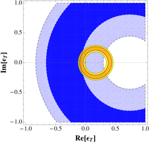
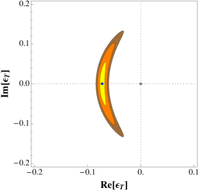
Figure 3: (left) Regions in the $(Re(\epsilon_{T}),Im(\epsilon_{T}))$ plane determined from the experimental data (to $1$ and $2\sigma$) on ${\cal R}(D)$ (large rings) and ${\cal R}(D^{*})$ (small rings). (right) Region corresponding to values of $\chi^{2}$ between the minimum (indicated by the star), $1.55$ (yellow, light) and $1.65$ (orange, gray) and $1.75$ (brown, dark).

Varying the effective coupling in this region we can analyze the impact of the new operator on various differential distributions.

We start with the longitudinal and transverse $D^{*}$ polarization distributions in $B\to D^{*}\tau{\bar{\nu}}_{\tau}$.

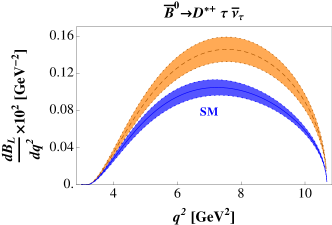
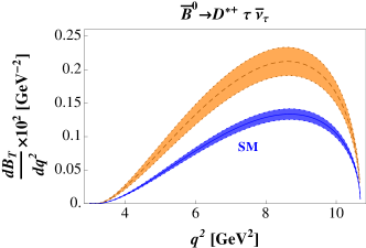
Figure 4: Differential branching ratios with polarized $D^{*}$: $\displaystyle{\frac{d{\cal B}(B\to D^{*}\tau{\bar{\nu}}_{\tau})_{L}}{dq^{2}}}$ (left) and $\displaystyle{\frac{d{\cal B}(B\to D^{*}\tau{\bar{\nu}}_{\tau})_{T}}{dq^{2}}}$ (right). The lower (blue) bands are the SM prediction, the upper (orange) bands include NP effects. In SM, the uncertainties on the parameters of the Isgur-Wise function in Eq.(51), together with the errors on $\overline{\Lambda}$ and $\alpha_{s}$ are included. In the case of the NP curves, the uncertainty on $\epsilon_{T}$ is also considered.

We consider the decay to a $D^{*}$ with definite helicity, with differential decay width $\displaystyle{\frac{d\Gamma_{L,\pm}}{dq^{2}}}$ for the three cases $L,\pm$. We define $\displaystyle{\frac{d\Gamma_{T}}{dq^{2}}=\frac{d\Gamma_{+}}{dq^{2}}+\frac{d\Gamma_{-}}{dq^{2}}}$ , and show in fig.4 the differential branching fractions. The uncertainty in the distributions reflects the uncertainty on the parameters of the Belle Isgur-Wise function, on $\bar{\Lambda}$ and, in the case of NP, on $\epsilon_{T}$. While the shape of the distributions are slightly modified from SM to NP, the maxima increase, a consequence of the increase of the branching fractions.

The differential decay width distributions for $D$ and $D^{*}$ (summed over the $D^{*}$ polarizations) have been measured by BaBar Lees:2013uzd , and can be compared to the SM and the NP scenario predictions. Once normalized to the total number of events, not only the SM distributions are compatible with data, as remarked in Lees:2013uzd , but also the distributions in the considered NP scenario agree with measurements, as one can argue considering fig.5. This confirms that the shape of such distributions does not allow at present to select between these possibilities, and other observables should be analyzed for a more efficient discrimination.

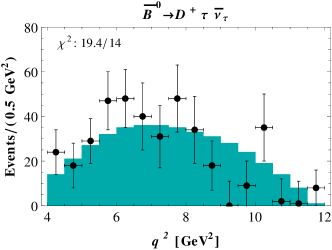
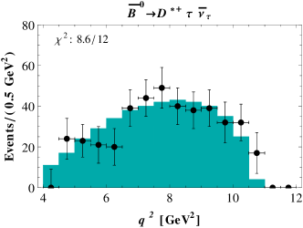
Figure 5: $\displaystyle{\frac{d\Gamma(B\to D\tau{\bar{\nu}}_{\tau})}{dq^{2}}}$ (left) and $\displaystyle{\frac{d\Gamma(B\to D^{*}\tau{\bar{\nu}}_{\tau})}{dq^{2}}}$ (right) distributions in the NP scenario (for the central value of $\epsilon_{T}$, shaded histograms) compared to BaBar data (points) Lees:2013uzd ; the distributions are normalized to the total number of events.

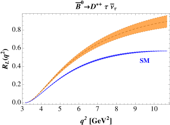
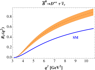
Figure 6: $D^{*}$ polarization ratios $R_{L}^{D^{*}}(q^{2})$ (left) and $R_{T}^{D^{*}}(q^{2})$ (right) defined in (57). Notations are the same as in fig.4.

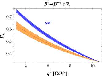
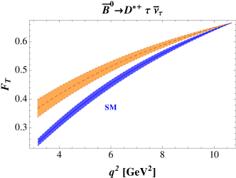
Figure 7: Polarization fractions $F_{L}(q^{2})$ (left) and $F_{T}(q^{2})$ (right) for $B\to D^{*}\tau{\bar{\nu}}_{\tau}$ defined in (58). Notations are the same as in fig.4.

Other observables are the longitudinal and transverse $D^{*}$ polarization distributions in $B\to D^{*}\tau{\bar{\nu}}_{\tau}$ normalized to $B\to D^{*}\ell{\bar{\nu}}_{\ell}$. They are defined as

$$R_{L,T}^{D^{*}}(q^{2})=\frac{d\Gamma_{L,T}(B\to D^{*}\tau{\bar{\nu}}_{\tau})/dq^{2}}{d\Gamma_{L,T}(B\to D^{*}\ell{\bar{\nu}}_{\ell})/dq^{2}}\,\,\,.$$ (57)

The SM predictions are shown in fig. 6 together with the modifications induced by the tensor operator. At large $q^{2}$ the observables are enhanced by $30-50$ $\%$, a noticeable effect. Furthermore, at odds with scenarios in which only $R_{L}$ is affected by new physics Celis:2012dk , in the case of the tensor operator both the longitudinal and the transverse $R_{L}$ and $R_{T}$ distributions are modified.

The longitudinal and transverse polarization fractions of the $D^{*}$ meson

$$F_{L,T}(q^{2})=\frac{d\Gamma_{L,T}(B\to D^{*}\tau{\bar{\nu}}_{\tau})}{dq^{2}}\times\left(\frac{d\Gamma(B\to D^{*}\tau{\bar{\nu}}_{\tau})}{dq^{2}}\right)^{-1}$$ (58)

are shown in fig.7. Both the SM and NP predictions are affected by a small error, since in the heavy quark limit the observables in (58) are free of hadronic uncertainties, due to the cancellation of the form factor $\xi(w)$ in the ratio. The residual uncertainty reflects that on $\bar{\Lambda}$ which controls the $1/m_{Q}$ corrections. The uncertainty on $\bar{\Lambda}$ also enters in the curves obtained in the NP scenario in combination with $\epsilon_{T}$. In SM, $F_{L}(q^{2})$ ranges between 0.75 at low $q^{2}$ and about 0.35 at high squared momentum transfer; in NP in the allowed region of $\epsilon_{T}$, $F_{L}(q^{2})$ is between 0.35 and about 0.65 at low $q^{2}$, while this observable converges to the SM value at high $q^{2}$. The SM predicts a dominant longitudinal polarization at small $q^{2}$, in NP the longitudinal and transverse polarizations have similar fractions up to $q^{2}=6$ GeV².

An important observable is the forward-backward ${\cal A}_{FB}(q^{2})$ asymmetry in $B\to D\tau{\bar{\nu}}_{\tau}$ and $B\to D^{*}\tau{\bar{\nu}}_{\tau}$, defined as

$${\cal A}_{FB}(q^{2})=\frac{\int_{0}^{1}\,d\cos\theta_{\ell}\,\frac{d\Gamma}{dq^{2}d\cos\theta_{\ell}}-\int_{-1}^{0}\,d\cos\theta_{\ell}\,\frac{d\Gamma}{dq^{2}d\cos\theta_{\ell}}}{\frac{d\Gamma}{dq^{2}}}\,\,\,,$$ (59)

where $\theta_{\ell}$ is the angle between the direction of the charged lepton and the $D^{(*)}$ meson in the lepton pair rest frame. We use the notation

$${\cal A}_{FB}(q^{2})=\frac{1}{\frac{d\Gamma}{dq^{2}}}\frac{3C(q^{2})}{16}\left\{\tilde{\cal A}_{FB}^{SM}(q^{2})+\tilde{\cal A}_{FB}^{NP}(q^{2})+\tilde{\cal A}_{FB}^{INT}(q^{2})\right\}\,\,\,,$$ (60)

with $C(q^{2})$ defined in (6) and the three terms in the parentheses given for $D$ and $D^{*}$:

• $D$

  $$\tilde{\cal A}_{FB}^{SM}(q^{2}) = 8F_{0}(q^{2})F_{1}(q^{2})(m_{B}^{2}-m_{D}^{2})\frac{m_{\ell}^{2}}{q^{2}}\left(1-\frac{m_{\ell}^{2}}{q^{2}}\right)\lambda^{1/2}(m_{B}^{2},m^{2},q^{2})$$

  $$\tilde{\cal A}_{FB}^{NP}(q^{2}) = 0$$

  $$\tilde{\cal A}_{FB}^{INT}(q^{2}) = -8Re(\epsilon_{T})F_{0}(q^{2})[F_{T}(q^{2})+G_{T}(q^{2})](m_{B}-m_{D})m_{\ell}\left(1-\frac{m_{\ell}^{2}}{q^{2}}\right)\lambda^{1/2}(m_{B}^{2},m^{2},q^{2})$$ (61)

• $D^{*}$

  $$\tilde{\cal A}_{FB}^{SM}(q^{2}) = \frac{4}{m_{D^{*}}(m_{B}+m_{D^{*}})q^{2}}\left(1-\frac{m_{\ell}^{2}}{q^{2}}\right)\lambda^{1/2}(m_{B}^{2},m_{D^{*}}^{2},q^{2})$$ (62)

  $$\Big{\{}m_{\ell}^{2}A_{0}(q^{2})\left[A_{1}(q^{2})(m_{B}+m_{D^{*}})^{2}(m_{B}^{2}-m_{D^{*}}^{2}-q^{2})-\lambda(m_{B}^{2},m_{D^{*}}^{2},q^{2})A_{2}(q^{2})\right]$$

  $$-4m_{D^{*}}(m_{B}+m_{D^{*}})q^{4}A_{1}(q^{2})V(q^{2})\Big{\}}$$

  $$\tilde{\cal A}_{FB}^{NP}(q^{2}) = 16|\epsilon_{T}|^{2}\frac{m_{\ell}^{2}}{q^{2}}\left(1-\frac{m_{\ell}^{2}}{q^{2}}\right)\lambda^{1/2}(m_{B}^{2},m_{D^{*}}^{2},q^{2})({\tilde{T}}_{1}(q^{2})+{\tilde{T}}_{2}(q^{2}))$$ (63)

  $$\left[(m_{B}^{2}-m_{D^{*}}^{2})({\tilde{T}}_{1}(q^{2})+{\tilde{T}}_{2}(q^{2}))+q^{2}({\tilde{T}}_{1}(q^{2})-{\tilde{T}}_{2}(q^{2}))\right]$$

  $$\tilde{\cal A}_{FB}^{INT}(q^{2}) = -4Re(\epsilon_{T})m_{\ell}\left(1-\frac{m_{\ell}^{2}}{q^{2}}\right)\lambda^{1/2}(m_{B}^{2},m_{D^{*}}^{2},q^{2})\Big{\{}4(m_{B}+m_{D^{*}})A_{1}(q^{2})({\tilde{T}}_{1}(q^{2})+{\tilde{T}}_{2}(q^{2}))$$ (64)

  $$+ A_{0}(q^{2})\left[\frac{\lambda(m_{B}^{2},m_{D^{*}}^{2},q^{2})}{m_{D^{*}}(m_{B}+m_{D^{*}})^{2}}{\tilde{T}}_{0}(q^{2})+2\frac{m_{B}^{2}+m_{D^{*}}^{2}-q^{2}}{m_{D^{*}}}{\tilde{T}}_{1}(q^{2})+4m_{D^{*}}{\tilde{T}}_{2}(q^{2})\right]$$

  $$- \frac{V(q^{2})}{m_{B}+m_{D^{*}}}\left[q^{2}({\tilde{T}}_{1}(q^{2})-{\tilde{T}}_{2}(q^{2}))+(m_{B}^{2}-m_{D^{*}}^{2})({\tilde{T}}_{1}(q^{2})+{\tilde{T}}_{2}(q^{2}))\right]\Big{\}}\,\,\,.$$

In fig.8 we plot ${\cal A}_{FB}(q^{2})$ for $B\to D\tau{\bar{\nu}}_{\tau}$ and $B\to D^{*}\tau{\bar{\nu}}_{\tau}$. The SM prediction is affected by almost no theoretical uncertainty, because of a nearly complete cancellation of the hadronic parameters in the ratio. In the case of NP, we have taken into account also the uncertainty on $\theta$ and $|a_{T}|$. The SM curve lies in both cases below the NP distribution for all values of $q^{2}$. The most interesting deviation concerns the $D^{*}$ mode: the SM predicts a zero for ${\cal A}_{FB}$ at $q^{2}\simeq 6.15$ GeV², in the NP case the zero is shifted towards larger values $q^{2}\in[8.1,9.3]$ GeV².

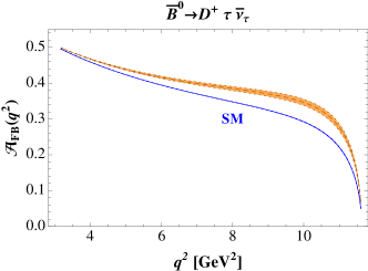
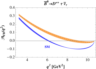
Figure 8: Forward-backward asymmetry ${\cal A}_{FB}(q^{2})$ for $B\to D\tau{\bar{\nu}}_{\tau}$ (left) and $B\to D^{*}\tau{\bar{\nu}}_{\tau}$ (right). The lower (blue) curves are the SM predictions, the upper (orange) bands the NP expectations. Uncertainty on $\overline{\Lambda}$ has been included and, in the case of NP, also on the parameters $|a_{T}|$ and $\theta$.

Even though the experimental determination of the zero of the forward-backward asymmetry is challenging, this observable effectively discriminates SM from the NP model. The integrated asymmetries, obtained integrating separately the numerator and the denominator in (59), are collected in Table 1: for $D^{*}$, in the NP scenario the integrated asymmetry has opposite sign with respect to SM.

	${\bar{B}}^{0}\to D^{+}\tau{\bar{\nu}}_{\tau}$	${\bar{B}}^{0}\to D^{*+}\tau{\bar{\nu}}_{\tau}$	${\bar{B}}^{0}\to D_{0}^{*+}\tau{\bar{\nu}}_{\tau}$	${\bar{B}}^{0}\to D_{1}^{\prime+}\tau{\bar{\nu}}_{\tau}$	${\bar{B}}^{0}\to D_{1}^{+}\tau{\bar{\nu}}_{\tau}$	${\bar{B}}^{0}\to D_{2}^{*+}\tau{\bar{\nu}}_{\tau}$
${\cal A}_{FB}^{SM}$	$0.357\pm 0.002$	$-0.040\pm 0.003$	$0.315$	$0.026$	$0.24$	$0.07$
${\cal A}_{FB}$	$0.40\pm 0.005$	$0.048\pm 0.013$	$0.30\pm 0.005$	$0.08\pm 0.01$	$0.21\pm 0.003$	$0.14\pm 0.01$

Table 1: Integrated forward-backward asymmetry for the considered decay modes. The first line reports the SM results, in the second line the effect of the tensor operator is included.

IV Tensor operator in $B\to D^{**}\ell{\bar{\nu}}_{\ell}$ decays

The new operator in the effective hamiltonian (4) affects other exclusive decay modes that are worth investigating. Of peculiar interest are the semileptonic $B$ and $B_{s}$ transitions into excited charmed mesons. The lightest multiplet of such hadrons, corresponding to the quark model $p$-wave ($\ell=1$) mesons and generically denoted $D_{(s)}^{**}$, comprises four positive parity states which, in the heavy quark limit, fill two doublets labeled by the (conserved) angular momentum ${\vec{s}}_{\ell}={\vec{s}}_{q}+{\vec{\ell}}$ (${\vec{s}}_{q}$ is spin of the light antiquark), hence $s_{\ell}=1/2$ or $s_{\ell}=3/2$. The two mesons belonging to the first doublet, $(D^{*}_{(s)0},\,D_{(s)1}^{\prime})$, have spin-parity $J^{P}=(0^{+},1^{+})$; the mesons in the second doublet have $J^{P}=(1^{+},2^{+})$ and are named $(D_{(s)1},\,D_{(s)2}^{*})$. All the members of the doublets, with and without strangeness, have been observed, and the two $s_{\ell}^{P}=1/2^{+}$ states without strangeness are found to be broad, as expected Colangelo:2012xi .

In the heavy quark limit also the semileptonic $B$ transitions to mesons belonging to the same charmed doublet can be described in terms of a single form factor. $B$ decays to $(D^{*}_{0},\,D_{1}^{\prime})$ are governed by a universal function denoted as $\tau_{1/2}(w)$, $B$ decays to $(D_{1},\,D_{2}^{*})$ by the $\tau_{3/2}(w)$ form factor (the matrix elements are collected in appendix B). There are several determinations of the $\tau_{i}(w)$ parametrized in terms of the zero-recoil value $\tau_{i}(1)$ (contrary to the Isgur-Wise function, $\tau_{i}(w)$ are not normalized to unity at $w=1$), of the slope $\rho_{i}^{2}$ and of the curvature $c_{i}$. In the ratios of branching fractions and asymmetries the zero-recoil value does not play any role, and this reduces the main dependence of the observables on the hadronic parameters. The present experimental situation needs to be settled, since the semileptonic $B$ decay rates into $(D^{*}_{0},\,D_{1}^{\prime})$ exceed the predictions obtained using computed $\tau_{i}(1)$; the origin of the discrepancy is still unknown, and could be related to the broad widths of the final charmed mesons, which determine a difficulty in the exclusive reconstruction, and to a possible pollution from other (e.g. radial) excited states. Semileptonic $B_{s}$ decays to $s_{\ell}^{P}=1/2^{+}$ $c\bar{s}$ mesons could clarify the issue, due to the narrow width of the strange charmed resonances Becirevic:2012te . On the other hand, the tensor operator produces precise correlations among various observables, therefore its effects could be distinguished from others.

For definiteness, we use a QCD sum rule determination of $\tau_{3/2}(w)$ at leading order in $\alpha_{s}$ Colangelo:1992kc ; Colangelo:1998sf , and of $\tau_{1/2}(w)$ at ${\cal O}(\alpha_{s})$ Colangelo:1998ga :

$$\tau_{3/2}(w) = \tau_{3/2}(1)\left[1-\rho^{2}_{3/2}(w-1)\right]$$ (65)

$$\tau_{1/2}(w) = \tau_{1/2}(1)\left[1-\rho^{2}_{1/2}(w-1)+c_{1/2}(w-1)^{2}\right]$$ (66)

with

$$\tau_{3/2}(1) = 0.28\hskip 56.9055pt\rho^{2}_{3/2}=0.9$$ (67)

$$\tau_{1/2}(1) = 0.35\pm 0.08\hskip 28.45274pt\rho^{2}_{1/2}=2.5\pm 1.0\hskip 28.45274ptc_{1/2}=3\pm 3\,\,.$$ (68)

The differential decay rates for $B\to D^{**}\ell{\bar{\nu}}_{\ell}$ can be written as in (5), see appendix B. The ratios

$${\cal R}(D^{*}_{0})=\frac{{\cal B}(B\to D^{*}_{0}\tau\,{\bar{\nu}}_{\tau})}{{\cal B}(B\to D^{*}_{0}\ell\,{\bar{\nu}}_{\ell})}$$ (69)

and the analogous ${\cal R}(D^{\prime}_{1})$, ${\cal R}(D_{1})$ and ${\cal R}(D^{*}_{2})$ depend on the effective coupling $\epsilon_{T}$. This also happens in $B_{s}\to D^{**}_{s}\ell{\bar{\nu}}_{\ell}$ transitions, in the $SU(3)_{F}$ symmetry limit for the form factors.

In fig.9 for each meson doublet we show the correlation between the ratios (69) for $B$ and $B_{s}$, together with the SM predictions $({\cal R}(D^{*}_{0}),{\cal R}(D^{\prime}_{1}))=(0.077,0.100)$, $({\cal R}(D^{*}_{s0}),{\cal R}(D^{\prime}_{s1}))=(0.107,0.112)$, $({\cal R}(D_{1}),{\cal R}(D^{*}_{2})=(0.065,0.059)$ and $({\cal R}(D_{s1}),{\cal R}(D^{*}_{s2})=(0.060,0.055)$. The tensor operator produces a sizeable increase in the ratios $\cal R$, which is correlated for the two members in each doublet. The hadronic uncertainty is mild: using the $\tau_{i}$ functions in Morenas:1997nk , the results remain almost unchanged in the case of the $s_{\ell}=3/2$ doublet, while for $s_{\ell}=1/2$ they are smaller by about $25\%$ in SM and in the NP case. The same effect is found using the form factors obtained by lattice QCD Blossier:2009vy .

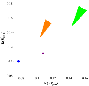
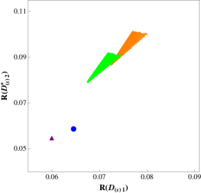
Figure 9: (left) Correlations between the ratios ${\cal R}(D^{*}_{(s)0})$ and ${\cal R}(D^{\prime}_{(s)1})$ for mesons belonging to the $(D^{*}_{(s)0},\,D_{(s)1}^{\prime})$ doublet without (orange, dark) and with strangeness (green, light). (right) Correlation between ${\cal R}(D_{(s)1})$ and ${\cal R}(D^{*}_{(s)2})$ for mesons in the $(D_{(s)1},\,D_{(s)2}^{*})$ doublet. The dots (triangles) correspond to the SM results for mesons without (with) strangeness.

The differential forward-backward asymmetries in the case of the four positive parity charmed mesons are collected in fig.10, and the integrated ones in Table 1.

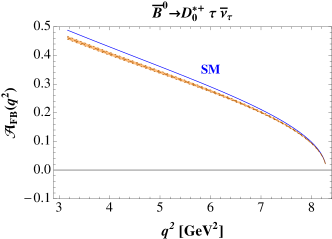
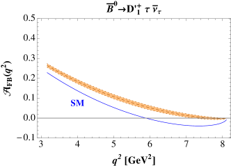
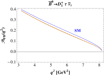
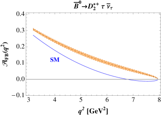
Figure 10: Forward-backward asymmetry ${\cal A}_{FB}$ for the decays $B\to D_{0}^{*}\tau{\bar{\nu}}_{\tau}$ (top, left), $B\to D^{\prime}_{1}\tau{\bar{\nu}}_{\tau}$ (top, right), $B\to D_{1}\tau{\bar{\nu}}_{\tau}$ (bottom, left) and $B\to D^{*}_{2}\tau{\bar{\nu}}_{\tau}$ bottom, (right) as function of $q^{2}$. The solid (blue) curves are the SM predictions, the dotted (orange) bands the NP expectations.

While in $B\to(D^{*}_{0},D_{1})\tau{\bar{\nu}}_{\tau}$ the forward-backward asymmetry does not discriminate between SN and NP, in the modes with $D_{1}^{\prime}$ and $D_{2}^{*}$ it is a sensitive observable: The inclusion of the tensor operator produces an enhancement of ${\cal A}_{FB}$ with respect to SM for all values of $q^{2}$. Moreover, in SM there is a zero which, in the case of $B\to D^{\prime}_{1}\tau{\bar{\nu}}_{\tau}$ moves towards larger values of $q^{2}$, and disappears in $B\to D^{*}_{2}\tau{\bar{\nu}}_{\tau}$ once NP is included.

We close this section remarking that, while the tensor operator in (4) does not affect the purely leptonic $B_{c}\to\tau^{-}{\bar{\nu}}_{\tau}$ mode, it can have an impact on the transitions $B_{c}\to(\eta_{c},J/\psi)\tau^{-}{\bar{\nu}}_{\tau}$ and $\Lambda_{b}\to\Lambda_{c}\tau^{-}{\bar{\nu}}_{\tau}$; therefore, sets of other observables can be identified and investigated, with precise correlated deviations from the SM predictions.

V Conclusions

The detailed experimental information provided us on flavour physics shows an astonishing consistency with the SM predictions. The very few tensions identify possible paths to new physics searches. The BaBar anomalous enhancement of the ratios $\displaystyle R(D^{(*)})=\frac{{\cal B}(B\to D^{(*)}\tau{\bar{\nu}}_{\tau})}{{\cal B}(B\to D^{(*)}\mu{\bar{\nu}}_{\mu})}$ with respect to SM is one of these few cases. The analyses of $R(D^{(*)})$ in specific models also evidentiate the enhancement the purely leptonic $B\to\tau{\bar{\nu}}_{\tau}$ rate, for which data are better compatible with SM. A mechanism enhancing the semileptonic modes $B\to D^{(*)}\tau{\bar{\nu}}_{\tau}$ with respect to $B\to D^{(*)}\mu{\bar{\nu}}_{\mu}$, leaving $B\to\tau{\bar{\nu}}_{\tau}$ unaffected, can be based on a tensor operator in the effective hamiltonian. We have bound the relative weight $\epsilon_{T}$ of this operator and studied the impact on several observables, the most sensitive one being the forward-backward asymmetry in $B\to D^{*}\tau{\bar{\nu}}_{\tau}$ with a shift in the position of its zero. If the anomaly in $B\to D^{(*)}\tau{\bar{\nu}}_{\tau}$ is due to this NP effect, analogous deviations should be found in B to excited $D$ transitions. The ratios $R$ for these mesons are enhanced with respect to SM, and the forward-backward asymmetry is a sensitive observable in the channels involving $D_{1}^{\prime}$ and $D_{2}^{*}$. These signatures in exclusive semileptonic $b\to c\,\tau{\bar{\nu}}_{\tau}$ modes make the understanding of the role of the new contribution to the effective weak hamiltonian feasible, a step towards possibly disclosing new interactions through flavour physics measurements.

Appendix A Coefficients

With the aim of providing the information useful to reconstruct the various $B\to D^{(*)}$ matrix elements, we collect here the expressions of the $\alpha_{s}$ and $1/m_{Q}$ corrections in Eqs.(21,22) and (40-43) worked out by M. Neubert and by I. Caprini et al. in hqet ; Caprini:1997mu . The functions $L_{i}(w)$ read as

$$L_{1} \simeq 0.72\,(w-1)\,{\bar{\Lambda}}$$

$$L_{2} \simeq -0.16\,(w-1)\,{\bar{\Lambda}}$$

$$L_{3} \simeq -0.24\,{\bar{\Lambda}}$$

$$L_{4} \simeq 0.24\,{\bar{\Lambda}}$$ (70)

$$L_{5} \simeq -{\bar{\Lambda}}$$

$$L_{6} \simeq -{3.24\over w+1}\,{\bar{\Lambda}}\,\,\,.$$

The coefficients $C_{i}$ are expressed in terms of $C_{1}$,

$${C_{1}^{5}\over C_{1}} = 1-{4\alpha_{s}\over 3\pi}r_{f}(w)$$

$${C_{2}^{(5)}\over C_{1}} = -{2\alpha_{s}\over 3\pi}H_{(5)}\left(w,\frac{1}{z_{m}}\right)$$ (71)

$${C_{3}^{(5)}\over C_{1}} = \mp{2\alpha_{s}\over 3\pi}H_{(5)}(w,z_{m})\,\,\,,$$

with $z_{m}={m_{c}\over m_{b}}$ and

$$r_{f}(w) = {1\over\sqrt{w^{2}-1}}\log\left[w+\sqrt{w^{2}-1}\right]\,\,\,\,,$$ (72)

$$H_{(5)}(w,z_{m}) = {z_{m}(1-\log z_{m}\mp z_{m})\over 1-2wz_{m}+z_{m}^{2}}+{z_{m}\over(1-2wz_{m}+z_{m}^{2})^{2}}\Big{[}2(w\mp 1)z_{m}(1\pm z_{m})\log z_{m}$$ (73)

$$- [(w\pm 1)-2w(2w\pm 1)z_{m}+(5w\pm 2w^{2}\mp 1)z_{m}^{2}-2z_{m}^{3}]r_{f}(w)\Big{]}\,\,\,.$$

In (71,73) the lower signs refer to the index $5$ (corresponding to the axial current). $C_{1}$ reads:

$$C_{1}=\left({\alpha_{s}(m_{c})\over\alpha_{s}(\mu)}\right)^{a_{hh}(w)}\left(1-{\alpha_{s}(\mu)\over\pi}Z_{hh}(w)\right)\left(1+{\alpha_{s}(m_{c})\over\pi}\left[\log\left(\frac{m_{b}}{m_{c}}\right)+Z_{hh}(w)+{2\over 3}[f(w)+r_{f}(w)+g(w)]\right]\right)\,\,\,,$$ (74)

with

$$a_{hh}(w) = {8\over 27}[w\,r_{f}(w)-1]\,\,\,,$$ (75)

$$Z_{hh}(w) = {8\over 81}\left({94\over 9}-\pi^{2}\right)(w-1)-{4\over 135}\left({92\over 9}-\pi^{2}\right)(w-1)^{2}+{\cal O}((w-1)^{3})\,\,\,,$$ (76)

$$f(w) = wr_{f}(w)-2-{w\over\sqrt{w^{2}-1}}[L_{2}(1-w_{-}^{2})+(w^{2}-1)r_{f}^{2}(w)]\,\,\,\,,$$ (77)

$$g(w) = {w\over\sqrt{w^{2}-1}}[L_{2}(1-z_{m}w_{-})-L_{2}(1-z_{m}w_{+})]-{z_{m}\over(1-2wz_{m}+z_{m}^{2})}[(w^{2}-1)r_{f}(w)+(w-z_{m})\log(z_{m})]\,\,\,,$$

and $w_{\pm}=w\pm\sqrt{w^{2}-1}$. In the numerical analysis we set the scale $\mu=\sqrt{m_{c}\,m_{b}}$, and investigate the sensitivity to higher order corrections varying this scale between $\mu/2$ and $2\mu$.

Appendix B $B\to D^{**}$ matrix elements and differential semileptonic decay rates

In the infinite heavy quark mass limit the $B\to D^{**}$ matrix elements can be defined in terms of two universal $\tau_{1/2}(w)$ and $\tau_{3/2}(w)$ form factors:

$$<D^{*}_{0}(p^{\prime})|{\bar{c}}\gamma_{\mu}(1-\gamma_{5})b|B(p)> = -2\sqrt{m_{B}m_{D^{*}_{0}}}\,\tau_{1/2}(w)\,\left(v-v^{\prime}\right)_{\mu}\,\,\,;$$ (79)

$$<D^{*}_{0}(p^{\prime})|{\bar{c}}\sigma_{\mu\nu}(1-\gamma_{5})b|B(p)> = 2\sqrt{m_{B}m_{D^{*}_{0}}}\,\tau_{1/2}(w)\,\left[-\epsilon_{\mu\nu\alpha\beta}v^{\alpha}v^{\prime\beta}+i(v_{\mu}v^{\prime}_{\nu}-v_{\nu}v^{\prime}_{\mu})\right]\,\,\,;$$ (80)

$$<D^{\prime}_{1}(p^{\prime},\,\epsilon)|{\bar{c}}\gamma_{\mu}(1-\gamma_{5})b|B(p)> = -2\sqrt{m_{B}m_{D^{\prime}_{1}}}\,\tau_{1/2}(w)\,\left[-i\epsilon_{\mu\alpha\beta\sigma}\epsilon^{*\alpha}v^{\beta}v^{\prime\sigma}-(w-1)\epsilon^{*}_{\mu}+(\epsilon^{*}\cdot v)v^{\prime}_{\mu}\right]\,\,\,;$$ (81)

$$<D^{\prime}_{1}(p^{\prime},\,\epsilon)|{\bar{c}}\sigma_{\mu\nu}(1-\gamma_{5})b|B(p)> = -2\sqrt{m_{B}m_{D^{\prime}_{1}}}\,\tau_{1/2}(w)\,\left\{-\epsilon_{\mu\nu\alpha\beta}\epsilon^{*\alpha}(v-v^{\prime})^{\beta}+i[\epsilon^{*}_{\mu}(v-v^{\prime})_{\nu}-\epsilon^{*}_{\nu}(v-v^{\prime})_{\mu}]\right\}\,\,\,;$$

$$<D_{1}(p^{\prime},\,\epsilon)|{\bar{c}}\gamma_{\mu}(1-\gamma_{5})b|B(p)> = \frac{\sqrt{m_{B}m_{D_{1}}}}{\sqrt{2}}\,\tau_{3/2}(w)\,\Big{\{}i(1+w)\epsilon_{\mu\alpha\beta\sigma}\epsilon^{*\alpha}v^{\beta}v^{\prime\sigma}+(w^{2}-1)\epsilon^{*}_{\mu}$$ (83)

$$+ (\epsilon^{*}\cdot v)\left[3v_{\mu}-(w-2)v^{\prime}_{\mu}\right]\Big{\}}\,\,\,;$$

$$<D_{1}(p^{\prime},\,\epsilon)|{\bar{c}}\sigma_{\mu\nu}(1-\gamma_{5})b|B(p)> = \frac{\sqrt{m_{B}m_{D_{1}}}}{\sqrt{2}}\,\tau_{3/2}(w)\,\Big{\{}-(w-1)\epsilon_{\mu\nu\alpha\beta}\epsilon^{*\alpha}(v+v^{\prime})^{\beta}+(\epsilon^{*}\cdot v)\epsilon_{\mu\nu\alpha\beta}v^{\alpha}v^{\prime\beta}$$ (84)

$$+ 2\epsilon_{\tau\sigma\alpha\beta}\epsilon^{*\sigma}v^{\alpha}v^{\prime\beta}\left[g^{\tau}_{\mu}v_{\nu}-g^{\tau}_{\nu}v_{\mu}\right]$$

$$+ i\left[(1+w)\left(\epsilon^{*}_{\nu}(v-v^{\prime})_{\mu}-\epsilon^{*}_{\mu}(v-v^{\prime})_{\nu}\right)-3(\epsilon^{*}\cdot v)(v_{\mu}v^{\prime}_{\nu}-v_{\nu}v^{\prime}_{\mu})\right]\Big{\}}\,\,\,;$$

$$<D_{2}^{*}(p^{\prime},\,\epsilon)|{\bar{c}}\gamma_{\mu}(1-\gamma_{5})b|B(p)> = \sqrt{m_{B}m_{D_{2}^{*}}}\,\sqrt{3}\,\tau_{3/2}(w)\,\Big{\{}-i\epsilon_{\mu\beta\tau\sigma}\left(\epsilon^{*\alpha\beta}v_{\alpha}\right)v^{\tau}v^{\prime\sigma}$$ (85)

$$+ \left(\epsilon^{*\alpha\beta}v_{\alpha}\right)v_{\beta}v^{\prime}_{\mu}-(1+w)\left(\epsilon^{*\alpha}_{\mu}v_{\alpha}\right)\Big{\}}\,\,\,;$$

$$<D_{2}^{*}(p^{\prime},\,\epsilon)|{\bar{c}}\sigma_{\mu\nu}(1-\gamma_{5})b|B(p)> = \sqrt{m_{B}m_{D_{2}^{*}}}\,\sqrt{3}\,\tau_{3/2}(w)\,\Big{\{}-\epsilon_{\mu\nu\beta\tau}\left(\epsilon^{*\alpha\beta}v_{\alpha}\right)(v+v^{\prime})^{\tau}$$ (86)

$$+ i\left(\epsilon^{*\alpha\tau}v_{\alpha}\right)\left[g^{\tau}_{\mu}(v+v^{\prime})_{\nu}-g^{\tau}_{\nu}(v+v^{\prime})_{\mu}\right]\Big{\}}\,\,\,.$$

In the previous formulae we have set $p=m_{B}\,v$, $p^{\prime}=m_{D^{**}}\,v^{\prime}$ and $w=v\cdot v^{\prime}$; $\epsilon$ is the polarization vector (tensor) of the spin 1 (spin 2) $D^{**}$ meson.

The results for the SM, NP and interference contribution to the differential distributions in (5) are given below for each of the four excited mesons. The relation between the squared momentum transfer $q^{2}$ and $w$ is $q^{2}=m_{B}^{2}+m_{D^{**}}^{2}-2m_{B}m_{D^{**}}w$, with $m_{D^{**}}$ the mass of the charmed meson produced in the decay. The lepton mass has been taken into account, hence the formulae also hold for $\tau$.

• $B\to D^{*}_{0}\ell{\bar{\nu}}_{\ell}$:

  $${d\tilde{\Gamma}\over dq^{2}}(B\to D^{*}_{0}\ell\bar{\nu}_{\ell})\Big{|}_{SM} = 4m_{B}m_{D_{0}^{*}}[\tau_{1/2}(w)]^{2}(w-1)\Big{\{}q^{2}\left(1-\frac{m_{\ell}^{2}}{q^{2}}\right)+\left(1+\frac{2m_{\ell}^{2}}{q^{2}}\right)\left[(m_{B}^{2}+m_{D_{0}^{*}}^{2})w-2m_{B}m_{D_{0}^{*}}\right]\Big{\}}$$

  $${d\tilde{\Gamma}\over dq^{2}}(B\to D^{*}_{0}\ell\bar{\nu}_{\ell})\Big{|}_{NP} = 32|\epsilon_{T}|^{2}m_{B}m_{D_{0}^{*}}[\tau_{1/2}(w)]^{2}(w^{2}-1)\left(1+\frac{2m_{\ell}^{2}}{q^{2}}\right)(m_{B}^{2}+m_{D_{0}^{*}}^{2}-2m_{B}m_{D_{0}^{*}}w)$$ (87)

  $${d\tilde{\Gamma}\over dq^{2}}(B\to D^{*}_{0}\ell\bar{\nu}_{\ell})\Big{|}_{INT} = -48Re(\epsilon_{T})m_{B}m_{D_{0}^{*}}[\tau_{1/2}(w)]^{2}(w^{2}-1)m_{\ell}(m_{B}-m_{D_{0}^{*}})$$

• $B\to D^{\prime}_{1}\ell{\bar{\nu}}_{\ell}$:

  $${d\tilde{\Gamma}\over dq^{2}}(B\to D^{\prime}_{1}\ell\bar{\nu}_{\ell})\Big{|}_{SM} = 4m_{B}m_{D_{1}^{\prime}}[\tau_{1/2}(w)]^{2}(w-1)$$

  $$\Big{\{}q^{2}\left(1-\frac{m_{\ell}^{2}}{q^{2}}\right)(2w-1)+\left(1+\frac{2m_{\ell}^{2}}{q^{2}}\right)\left[(m_{B}^{2}+m_{D_{1}^{\prime}}^{2})3w-2m_{B}m_{D_{1}^{\prime}}(2w^{2}+1)\right]\Big{\}}$$

  $${d\tilde{\Gamma}\over dq^{2}}(B\to D^{\prime}_{1}\ell\bar{\nu}_{\ell})\Big{|}_{NP} = 32|\epsilon_{T}|^{2}m_{B}m_{D_{1}^{\prime}}[\tau_{1/2}(w)]^{2}(w-1)\left(1+\frac{2m_{\ell}^{2}}{q^{2}}\right)$$ (88)

  $$\Big{\{}(m_{B}^{2}+m_{D_{1}^{\prime}}^{2})(5w-1)-2m_{B}m_{D_{1}^{\prime}}[4+w(w-1)]\Big{\}}$$

  $${d\tilde{\Gamma}\over dq^{2}}(B\to D^{\prime}_{1}\ell\bar{\nu}_{\ell})\Big{|}_{INT} = 48Re(\epsilon_{T})m_{B}m_{D_{1}^{\prime}}[\tau_{1/2}(w)]^{2}(w-1)m_{\ell}[m_{B}(w-5)+m_{D_{1}^{\prime}}(5w-1)]$$

• $B\to D_{1}\ell{\bar{\nu}}_{\ell}$:

  $${d\tilde{\Gamma}\over dq^{2}}(B\to D_{1}\ell\bar{\nu}_{\ell})\Big{|}_{SM} = m_{B}m_{D_{1}}[\tau_{3/2}(w)]^{2}(w-1)(1+w)^{2}$$

  $$\Big{\{}q^{2}\left(1-\frac{m_{\ell}^{2}}{q^{2}}\right)(w-2)+\left(1+\frac{2m_{\ell}^{2}}{q^{2}}\right)\left[(m_{B}^{2}+m_{D_{1}}^{2})3w-2m_{B}m_{D_{1}}(w^{2}+2)\right]\Big{\}}$$

  $${d\tilde{\Gamma}\over dq^{2}}(B\to D_{1}\ell\bar{\nu}_{\ell})\Big{|}_{NP} = 16|\epsilon_{T}|^{2}m_{B}m_{D_{1}}[\tau_{3/2}(w)]^{2}(w-1)(1+w)^{2}\left(1+\frac{2m_{\ell}^{2}}{q^{2}}\right)$$ (89)

  $$\Big{\{}\left[(m_{B}^{2}+m_{D_{1}}^{2})(2w-1)-2m_{B}m_{D_{1}}(w^{2}-w+1)\right]\Big{\}}$$

  $${d\tilde{\Gamma}\over dq^{2}}(B\to D_{1}\ell\bar{\nu}_{\ell})\Big{|}_{INT} = 24Re(\epsilon_{T})m_{B}m_{D_{1}}[\tau_{3/2}(w)]^{2}(w-1)(1+w)^{2}m_{\ell}[m_{B}(w-2)+m_{D_{1}}(2w-1)]$$

• $B\to D^{*}_{2}\ell{\bar{\nu}}_{\ell}$:

  $${d\tilde{\Gamma}\over dq^{2}}(B\to D^{*}_{2}\ell\bar{\nu}_{\ell})\Big{|}_{SM} = m_{B}m_{D^{*}_{2}}[\tau_{3/2}(w)]^{2}(w-1)(1+w)^{2}$$

  $$\Big{\{}q^{2}\left(1-\frac{m_{\ell}^{2}}{q^{2}}\right)(3w+2)+\left(1+\frac{2m_{\ell}^{2}}{q^{2}}\right)\left[(m_{B}^{2}+m_{D^{*}_{2}}^{2})5w-2m_{B}m_{D^{*}_{2}}(3w^{2}+2)\right]\Big{\}}$$

  $${d\tilde{\Gamma}\over dq^{2}}(B\to D^{*}_{2}\ell\bar{\nu}_{\ell})\Big{|}_{NP} = 16|\epsilon_{T}|^{2}m_{B}m_{D^{*}_{2}}[\tau_{3/2}(w)]^{2}(w-1)(1+w)^{2}\left(1+\frac{2m_{\ell}^{2}}{q^{2}}\right)$$ (90)

  $$\Big{\{}\left[(m_{B}^{2}+m_{D^{*}_{2}}^{2})(1+4w)-2m_{B}m_{D^{*}_{2}}(3+w+w^{2})\right]\Big{\}}$$

  $${d\tilde{\Gamma}\over dq^{2}}(B\to D^{*}_{2}\ell\bar{\nu}_{\ell})\Big{|}_{INT} = -24Re(\epsilon_{T})m_{B}m_{D^{*}_{2}}[\tau_{3/2}(w)]^{2}(w-1)(1+w)^{2}m_{\ell}[m_{B}(4+w)-m_{D^{*}_{2}}(1+4w)]$$

The differential decay rates are obtained multiplying the above functions by the coefficient $C(q^{2})$ in (6).

References

- (1) J. P. Lees et al. [BaBar Collaboration], Phys. Rev. Lett. 109, 101802 (2012) [arXiv:1205.5442 [hep-ex]].
- (2) S. Fajfer, J. F. Kamenik and I. Nisandzic, Phys. Rev. D 85, 094025 (2012) [arXiv:1203.2654 [hep-ph]].
- (3) S. Fajfer, J. F. Kamenik, I. Nisandzic and J. Zupan, Phys. Rev. Lett. 109, 161801 (2012) [arXiv:1206.1872 [hep-ph]].
- (4) A. Crivellin, C. Greub and A. Kokulu, Phys. Rev. D 86, 054014 (2012) [arXiv:1206.2634 [hep-ph]].
- (5) A. Datta, M. Duraisamy and D. Ghosh, Phys. Rev. D 86, 034027 (2012) [arXiv:1206.3760 [hep-ph]].
- (6) D. Becirevic, N. Kosnik and A. Tayduganov, Phys. Lett. B 716, 208 (2012) [arXiv:1206.4977 [hep-ph]].
- (7) A. Celis, M. Jung, X. -Q. Li and A. Pich, JHEP 1301, 054 (2013) [arXiv:1210.8443 [hep-ph]].
- (8) D. Choudhury, D. K. Ghosh and A. Kundu, Phys. Rev. D 86, 114037 (2012) [arXiv:1210.5076 [hep-ph]].
- (9) M. Tanaka and R. Watanabe, arXiv:1212.1878 [hep-ph].
- (10) J. Laiho, E. Lunghi and R. S. Van de Water, Phys. Rev. D 81, 034503 (2010) [arXiv:0910.2928 [hep-ph]] and the average quoted in http://latticeaverages.org/ .
- (11) M. Bona et al. [UTfit Collaboration], Phys. Lett. B 687, 61 (2010) [arXiv:0908.3470 [hep-ph]].
- (12) A. Lenz, U. Nierste, J. Charles, S. Descotes-Genon, A. Jantsch, C. Kaufhold, H. Lacker and S. Monteil et al., Phys. Rev. D 83, 036004 (2011) [arXiv:1008.1593 [hep-ph]].
- (13) B. Aubert et al. [BABAR Collaboration], Phys. Rev. D 77, 011107 (2008) [arXiv:0708.2260 [hep-ex]].
- (14) B. Aubert et al. [BABAR Collaboration], Phys. Rev. D 81, 051101 (2010) [arXiv:0912.2453 [hep-ex]].
- (15) K. Ikado et al. [Belle Collaboration], Phys. Rev. Lett. 97, 251802 (2006) [hep-ex/0604018].
- (16) K. Hara et al. [Belle Collaboration], Phys. Rev. D 82, 071101 (2010) [arXiv:1006.4201 [hep-ex]].
- (17) J. L. Rosner and S. Stone, arXiv:1201.2401 [hep-ex].
- (18) I. Adachi et al. [Belle Collaboration], arXiv:1208.4678 [hep-ex].
- (19) J. P. Lees et al. [BABAR Collaboration], arXiv:1207.0698 [hep-ex].
- (20) H. Georgi and S. L. Glashow, Phys. Rev. Lett. 32, 438 (1974); S. Chakdar, T. Li, S. Nandi and S. K. Rai, Phys. Lett. B 718, 121 (2012) [arXiv:1206.0409 [hep-ph]].
- (21) J. C. Pati and A. Salam, Phys. Rev. D 10, 275 (1974) [Erratum-ibid. D 11, 703 (1975)].
- (22) B. Schrempp and F. Schrempp, Phys. Lett. B 153, 101 (1985); W. Buchmuller, R. Ruckl and D. Wyler, Phys. Lett. B 191, 442 (1987) [Erratum-ibid. B 448, 320 (1999)].
- (23) J. L. Hewett and T. G. Rizzo, Phys. Rept. 183, 193 (1989).
- (24) S. Dimopoulos and L. Susskind, Nucl. Phys. B 155, 237 (1979); S. Dimopoulos, Nucl. Phys. B 168, 69 (1980); E. Eichten and K. D. Lane, Phys. Lett. B 90, 125 (1980).
- (25) [CMS Collaboration], report CMS-PAS-EXO-12-002.
- (26) S. Rolli and M. Tanabashi, review Leptoquarks in pdg .
- (27) J. Beringer et al. [Particle Data Group Collaboration], Phys. Rev. D 86, 010001 (2012).
- (28) N. Isgur and M. B. Wise, Phys. Lett. B 237, 527 (1990).
- (29) M. Neubert, Phys. Rept. 245, 259 (1994).
- (30) F. De Fazio, in At the Frontier of Particle Physics/Handbook of QCD, ed. by M. Shifman (World Scientific, Singapore, 2001), page 1671, arXiv:hep-ph/0010007; A. V. Manohar and M. B. Wise, Camb. Monogr. Part. Phys. Nucl. Phys. Cosmol. 10, 1 (2000).
- (31) B. Aubert et al. [BABAR Collaboration], Phys. Rev. Lett. 104, 011802 (2010) [arXiv:0904.4063 [hep-ex]].
- (32) I. Caprini, L. Lellouch and M. Neubert, Nucl. Phys. B 530, 153 (1998) [hep-ph/9712417].
- (33) W. Dungel et al. [Belle Collaboration], Phys. Rev. D 82, 112007 (2010) [arXiv:1010.5620 [hep-ex]].
- (34) J. P. Lees et al. [BABAR Collaboration], arXiv:1303.0571 [hep-ex].
- (35) A comprehensive analysis of the open charm meson spectrum can be found in P. Colangelo, F. De Fazio, F. Giannuzzi and S. Nicotri, Phys. Rev. D 86, 054024 (2012) [arXiv:1207.6940 [hep-ph]].
- (36) D. Becirevic, A. Le Yaouanc, L. Oliver, J. -C. Raynal, P. Roudeau and J. Serrano, arXiv:1206.5869 [hep-ph].
- (37) P. Colangelo, G. Nardulli and N. Paver, Phys. Lett. B 293, 207 (1992).
- (38) P. Colangelo, F. De Fazio and N. Paver, Nucl. Phys. Proc. Suppl. 75B, 83 (1999) [hep-ph/9809586].
- (39) P. Colangelo, F. De Fazio and N. Paver, Phys. Rev. D 58, 116005 (1998) [hep-ph/9804377].
- (40) V. Morenas, A. Le Yaouanc, L. Oliver, O. Pene and J. C. Raynal, Phys. Rev. D 56, 5668 (1997) [hep-ph/9706265].
- (41) B. Blossier et al. [European Twisted Mass Collaboration], JHEP 0906 (2009) 022 [arXiv:0903.2298 [hep-lat]].