Wigner dynamics of quantum semi-relativistic oscillator

Abstract

The integral Wigner - Liouwille equation describing time evolution of the semi-relativistic quantum 1D harmonic oscillator have been exactly solved by combination of the Monte-Carlo procedure and molecular dynamics methods. The strong influence of the relativistic effects on the time evolution of the momentum, velocity and coordinate Wigner distribution functions and the average values of quantum operators have been studied. Unexpected ’protuberances’ in time evolution of the distribution functions were observed. Relativistic proper time dilation for oscillator have been calculated.

I Introduction

The harmonic oscillator concept occupies a central position in science and engineering due to its simplicity and exact solubility in both classical and quantum descriptions. Today it appears in mechanics, electromagnetism, electronics, optics, acoustics, astronomy, nuclear theory and so on. In the quantum approach the harmonic oscillator is one of the exactly solvable problems studied in detail due to its considerable physical interest and applicability. The problem of a one-dimensional harmonic oscillator is also one of the important paradigms leading to the enormous applications in a wide range of the modern physics HO .

There are at least three logically autonomous alternative paths to quantization. The first is the standard one utilizing operators in Hilbert space, developed by Heisenberg, Schrodinger, Dirac, and others in the 1920s. The second one relies on path integrals, and was conceived by Dirac and constructed by Feynman feynm . The third one is the phase-space formulation. It is based on Wigner s (1932) quasi-distribution function and Weyl s (1927) correspondence between ordinary c-number functions in phase space and quantum mechanical operators in Hilbert space tatr1 . This complete formulation is based on the Wigner function (WF), which is a quasiprobability distribution function in phase-space.

Wigner s quasi-probability distribution function in phase-space is a special (Weyl- Wigner) representation of the density matrix. It has been useful in describing transport properties, quantum optics, nuclear physics, quantum computing, decoherence and chaos. It furnishes a third, alternative, formulation of quantum mechanics, independent of the conventional Hilbert space, or path integral formulations. In this logically complete and self-standing formulation, one need not choose sides between coordinate or momentum space. It works in full phase-space, accommodating the uncertainty principle; and it offers unique insights into the classical limit of quantum theory: The variables (observables) in this formulation are c-number functions in phase space instead of operators, with the same interpretation as their classical counterparts, but are composed together in novel algebraic ways.

The simplest and perhaps most straightforward generalization of nonrelativistic quantum theory towards the inclusion of relativistic kinematics leads to Hamiltonians $\hat{H}$ that involve the relativistic kinetic energy, or relativistically covariant form of the free energy, of a particle of mass $m$ and momentum $p$, given by the square-root operator and a coordinate-dependent static interaction potential $V(x)$, so $\hat{H}(\hat{p},\hat{x})=\sqrt{\hat{p}^{2}c^{2}+m^{2}c^{4}}+V(\hat{x}.)$ ($c$ is velocity of light in free space). The eigenvalue equation of this Hamiltonian is usually called the spinless Salpeter equation. It may be regarded as a well-defined approximation to the Bethe Salpeter formalism SB1 for the description of bound states within relativistic quantum field theories, obtained when assuming that all bound-state constituents interact instantaneously and propagate like free particles SB2 . Among others, it yields semi-relativistic descriptions of hadrons as bound states of quarks LS1 ; LS2 .

We study rigorously the semi-relativistic quantum 1D harmonic oscillator described by the Hamiltonian operator composed of the relativistic kinetic energy and a static harmonic potential using Wigner formulation of quantum mechanics. In this research we have considered a time evolution of such system, notably the time evolution of the momentum, coordinate and velocity distributions, average values of their quantum operators and relativistic time dilation. We used both Monte-Carlo procedure and method of molecular dynamic for numerical solution of this problem.

II Wigner - Lioville equation

Integral form of the Wigner - Lioville equation. The most conventional formulation of quantum mechanics is description of system’s dynamics with complex wave function. This function of particle with mass $m$ and moving in potential field $V(x)$ (we consider one dimension) satisfies the Schroedinger equation:

$$i\hbar\frac{\partial\Psi(q,t)}{\partial t}=\hat{H}\Psi(q,t)$$ (1)

,where hamiltonian is $\hat{H}=\hat{p}^{2}/2m+V(\hat{q})$ and the initial condition is $\Psi(q,0)=\Psi_{0}(q)$

More general description of quantum systems is given in terms of the density matrix $\rho(q,q^{\prime};t)$ (in coordinate representation), which has the following form in case of pure state: $\rho(q,q^{\prime};t)=\Psi(q,t)\Psi^{*}(q^{\prime},t)$. Evolution equation for density matrix is

$$i\hbar\frac{\partial\rho(q,q^{\prime};t)}{\partial t}=(\hat{H}-\hat{H}^{\prime*})\rho(q,q^{\prime};t),$$ (2)

where $\hat{H}$ acts on coordinate $q$, while $\hat{H}^{\prime}$ acts on coordinate $q^{\prime}$. The initial condition for this equation has form $\rho(q,q^{\prime};0)=\rho_{0}(q,q^{\prime})=\Psi_{0}(q)\Psi_{0}^{*}(q^{\prime})$.

In the Wigner representation of quantum mechanics we use joint distribution of quasiprobability for momentum and coordinate; it is called Wigner function tatr1 . Wigner function is defined as Fourier transform of density matrix on difference variable $\xi=q-q^{\prime}$, while center varible is $x=(q+q^{\prime})/2$:

$$W(x,p;t)=\frac{1}{2\pi\hbar}\int\limits_{-\infty}^{\infty}{\rho(x-\xi/2,x+\xi/2)e^{ip\xi/\hbar}}d{\xi}.$$ (3)

Evolution of quantum system in Wigner representation is describing by Wigner - Liouwille equation tatr1 :

$$\frac{\partial W(x,p;t)}{\partial t}+\frac{\partial H(p,x)}{\partial p}\frac{\partial W(x,p;t)}{\partial x}-\frac{\partial H(p,x)}{\partial x}\frac{\partial W(x,p;t)}{\partial p}=$$

$$\frac{1}{i\hbar}\left[V\left(x+\frac{i\hbar}{2}\frac{\partial}{\partial p}\right)-V\left(x-\frac{i\hbar}{2}\frac{\partial}{\partial p}\right)-i\hbar V^{\prime}_{x}(x)\frac{\partial}{\partial p}\right]W(x,p;t),$$ (4)

with initial condition $W(x,p;0)=W_{0}(x,p)$ defined by (3) at $t=0$. When the related to Hamiltonian the classical Hamilton’s function has the form $H(p,q)=p^{2}/2m+V(x)$, the partial derivatives are: $\partial H/\partial x=V^{\prime}_{x}(x)$, $\partial H/\partial p=p/m$.

In quantum mechanics Wigner functions are real valued but altering sign analog of the probabilistic joint $p$ and $x$ distributions in classical mechanics. This is supported by its general properties tatr1 : a) density of probability in momentum space is $W(p)=\int\limits_{-\infty}^{\infty}{}\,W(x,p)dx$; b) density of probability in configuration space is $W(x)=\int\limits_{-\infty}^{\infty}{}\,W(x,p)dp\quad$. In additition $W(x,p)$ is bilinear in wave function $\Psi(x,t)$ or in $\Psi(p,t)$ in momentum representation;

One can rewrite evolution equation (II) in the integral form tatr1 ; kmf :

$$W(x,p;t)=\int G(p,x,t;p_{0},x_{0},0)W_{0}(x_{0},p_{0})\,dp_{0}\,dx_{0}+$$

$$\int_{0}^{t}d\tau\int dp_{\tau}dx_{\tau}G\left(p,x,t;p_{\tau},x_{\tau},\tau\right)\int_{-\infty}^{\infty}ds\,W\left(x_{\tau},p_{\tau}-s,\tau\right)\omega\left(s,x_{\tau}\right)$$ (5)

with $\omega\left(s,x\right)=F\left(x\right)\frac{d\delta\left(s\right)}{ds}+\frac{4}{\left(2\pi\right)}\int d{q}\,V\left(x-q\right)\sin\left(2sq\right)$. Here $F\left(x\right)=-\partial V(x)/\partial x$ is the classical force. Here $G(p,x,t;p_{\tau},x_{\tau},\tau)$ is the Green’s function for classical Liouwille equation

$$G(p,x,t;p_{\tau},x_{\tau},\tau)=\delta(p-\bar{p}(t;\tau,p_{\tau},x_{\tau}))\delta(x-\bar{x}(t;\tau,p_{\tau},x_{\tau})),$$ (6)

where $\bar{p}$, $\bar{x}$ are solutions of Hamilton’s equations

$$\frac{dp}{dt}=-\frac{\partial H(p,x)}{\partial x},\qquad\frac{dx}{dt}=\frac{\partial H(p,x)}{\partial p},$$ (7)

with initial conditions $\bar{p}(\tau;\tau,p_{\tau},x_{\tau})=p_{\tau},\bar{x}(\tau;\tau,p_{\tau},x_{\tau})=x_{\tau},$.

Solution of equation (II) can be written in the form of the iterative series, which have the following interpretation. The first term of the series (the first term in the r.h.s of the Eqs II) is equal to the sum of the contributions of the virtual classical trajectories defined by the dynamical Hamilton’s equations (7). The contribution of the each virtual trajectory is equal to the value of the initial Wigner function $W_{0}(x_{0},p_{0})$ taken at initial point $x_{0},p_{0}$. Next terms of the iterative series are equal to the sum of the contributions of virtual trajectories consisting of segments of classical trajectories, separated by ’jumps’ in momentum. The term’s number in iterative series is equal to number of the momentum ’jumps’ as it follows from convolution structure of integral term in equation (II). In the classical limit ($\hbar\to 0$) the force term in $\omega$ cancels the last term and only the first term of iterative series gives the main contribution to solution of the Wigner-Liouville equation. In the classical limit Eqs. (II), (II) are reduced to the classical Liouville equations.

Restrictions on initial condition. To find solutions of the integral equation (II) the initial function $W_{0}(x,p)$ have to be taken according to the definition (3). However this definition imposes the certain restriction on the choice of possible functions in phase space. This can be easily illustrated for harmonic oscillator (particle in potential field $V(x)=V_{0}+V_{1}x+V_{2}x^{2}$ ). In this case the Wigner-Liouwille equation (II) is reduced to the form

$$\frac{\partial W(x,p;t)}{\partial t}+\frac{p}{m}\frac{\partial W(x,p;t)}{\partial x}-V^{\prime}_{x}(x)\frac{\partial W(x,p;t)}{\partial p}=0,$$ (8)

and coincides with the classical Liouwille equation. However solution of quantum harmonic oscillator is totally distinguished from classical one. Consequently, quantum and classical solutions of this task distinguish from each other in choice of the initial condition $W_{0}(x,p)$. So we need additional condition to choose classical or quantum solution. For density matrix of pure state this condition can be formulated as follows

$$\frac{\partial^{2}}{\partial x_{1}\partial x_{2}}\ln{\rho(x_{1},x_{2};0)}=0,\mbox{ or in Wigner representation \cite[cite]{\@@bibref{Authors Phrase1YearPhrase2}{tatr1}{\@@citephrase{(}}{\@@citephrase{)}}} }\quad\frac{\partial^{2}}{\partial x_{1}\partial x_{2}}ln\int\limits_{-\infty}^{\infty}W_{0}(\frac{x_{1}+x_{2}}{2},p)e^{ip(x_{1}-x_{2})/\hbar}\,dp.$$ (9)

In klim one can find another condition of the choice $W_{0}(x,p)$, which is equivalent to this one. One of the physical interpretation of this additional conditions is connected with requirement for mean-square coordinate and momentum deviations to satisfy Heisenberg’s principle of uncertainty at time equal to zero.

Physical quantities. To calculate the average value of physical quantity $<\hat{A}>$ corresponded to quantum operator $\hat{A}$ the Weil’s symbol $A(p,x)$ has to be introduced by expression tatr1 :

$$A(p,x)=\int\limits_{-\infty}^{\infty}{\exp{ip\xi/\hbar}\left\langle x-\frac{\xi}{2}\left|\hat{A}\right|x+\frac{\xi}{2}\right\rangle}\,d\xi\quad\mbox{then}\quad<\hat{A}>=\int{W(x,p)A(p,x)}\,dp\,dx,$$ (10)

where $W(x,p)$ is Wigner function.

Non-relativistic harmonic oscillator. Non-relativistic harmonic oscillator with mass $m$ and circular frequency $\omega$ has Hamiltonian

$$\hat{H}=\frac{\hat{p}^{2}}{2m}+\frac{m\omega^{2}\hat{x}^{2}}{2};$$ (11)

Wigner-Liouville equation (II) in case of harmonic potential $V(x)=m\omega^{2}x^{2}/2$ has a simple form:

$$\frac{\partial W(x,p;t)}{\partial t}+\frac{p}{m}\frac{\partial W(x,p;t)}{\partial x}-m\omega^{2}x\frac{\partial W(x,p;t)}{\partial p}=0,$$ (12)

As the initial condition for equations (12) we will consider a coherent state of harmonic oscillator given by the wave function quantum : $\Psi(x,0)=\left(\frac{m\omega}{\pi\hbar}\right)^{1/4}\exp{\left\{\frac{i\tilde{p}x}{\hbar}-\frac{m\omega(x-\tilde{x})^{2}}{2\hbar}\right\}}\exp{\left\{-\frac{i\tilde{p}\tilde{x}}{2\hbar}\right\}}.$ Here $\tilde{p}$,$\tilde{x}$ are average values of momentum and coordinate at the initial moment $t=0$. According to definition (3), the initial Wigner function is defined by:

$$W_{0}(x,p)=\frac{1}{\pi\hbar}\exp{\left\{-\frac{m\omega(x-\tilde{x})^{2}}{\hbar}-\frac{(p-\tilde{p})^{2}}{\hbar m\omega}\right\}}.$$ (13)

Solution of equation (12) as well as the related integral equation (II) can be written in the form

$$W(x,p;t)=\int(\delta(p-\bar{p}(t;0,p_{0},x_{0}))\delta(x-\bar{x}(t;0,p_{0},x_{0})))W_{0}(x_{0},p_{0})\,dp_{0}\,dx_{0}=$$

$$\frac{1}{\sqrt{2\pi(\hbar/2m\omega)}}\exp{\left\{-\frac{m\omega}{\hbar}[x-(\tilde{x}\cos{\omega t}+\frac{\tilde{p}}{m\omega}sin{\omega t})]^{2}-\frac{1}{\hbar m\omega}[p-(\tilde{p}cos{\omega t}-m\omega\tilde{x}sin{\omega t})]^{2}\right\}}.$$ (14)

where $\bar{p}(t)$, $\bar{x}(t)$ are virtual trajectories defined by the Hamilton’s function: $H(p,x)=\frac{p^{2}}{2m}+\frac{m\omega^{2}x^{2}}{2}$ and the Hamilton’s equations (7) with initial conditions $\bar{p}(0)=p_{0}$, $\bar{x}(0)=x_{0}$: $\,\bar{p}(t)=p_{0}\cos{\omega t}-m\omega x_{0}\sin{\omega t},\bar{x}(t)=\frac{p_{0}}{m\omega}\sin{\omega t}+x_{0}\cos{\omega t}.$

From (II) it follows that in a coherent state of harmonic oscillator the average momentum and coordinate satisfy classical law of motion $<p(t)>=\tilde{p}\cos{\omega t}-m\omega\tilde{x}\sin{\omega t},\qquad<x(t)>=\tilde{x}\cos{\omega t}+\frac{\tilde{p}}{m\omega}sin{\omega t}$  and the standard deviations of momentum and coordinate are constant: $<\delta p^{2}>=\frac{\hbar m\omega}{2},\qquad<\delta x^{2}>=\frac{\hbar}{2m\omega}$. While Heisenberg’s formula of uncertainty has it’s minimum: $<\delta p^{2}><\delta x^{2}>=\hbar^{2}/4$. Average energy is constant equal to $E=\frac{\hbar\omega}{2}+\frac{\tilde{p}^{2}}{2m}+\frac{m\omega^{2}\tilde{x}^{2}}{2}$.   More general case of the composite states slightly distinguished from pure coherent state is considered in kmf .

Semi-relativistic harmonic oscillator. The Hamiltonian of the semi-relativistic harmonic oscillator has the form:

$$\hat{H}=\sqrt{\hat{p}^{2}c^{2}+m^{2}c^{4}}+\frac{m\omega^{2}\hat{x}^{2}}{2}.$$ (15)

Wigner function has to be a solution of the Wigner - Lioville equation (II) tab3 :

$$\frac{\partial W(x,p;t)}{\partial t}+\frac{pc^{2}}{\sqrt{p^{2}c^{2}+m^{2}c^{4}}}\frac{\partial W(x,p;t)}{\partial x}-m\omega^{2}x\frac{\partial W(x,p;t)}{\partial p}=0,$$ (16)

with initial condition $W(x,p;0)=W_{0}(x,p)$ and the Hamilton’s function: $H(p,x)=\sqrt{p^{2}c^{2}+m^{2}c^{4}}+\frac{m\omega^{2}x^{2}}{2}.$

As before solution of this equation looks like:

$$W(x,p;t)=\int G(p,x,t;p_{0},x_{0},0)W_{0}(x_{0},p_{0})\,dp_{0}\,dx_{0},$$ (17)

where in the Green’s function the virtual trajectories $\bar{p}(t;t_{0},p_{0},x_{0})$ and $\bar{x}(t;t_{0},p_{0},x_{0})$ are solutions of Hamilton’s equations (7). When $c\to\infty$ the Hamilton’s function is equal to its non-relativistic limit (with rest energy term $mc^{2}$) $H\to{mc^{2}+\frac{p^{2}}{2m}+\frac{m\omega^{2}x^{2}}{2}}$.

Period of oscillations of the virtual trajectories versus energy have been found in tabl . Indeed from (7) one can obtained an equation for $p(t)$ and it’s first integral:

$$\frac{d^{2}\bar{p}}{dt^{2}}+m\omega^{2}c\frac{\bar{p}}{\sqrt{\bar{p}^{2}+m^{2}c^{2}}}=0,\qquad C_{1}=\left(\frac{d\bar{p}}{dt}\right)^{2}+2m\omega^{2}\sqrt{\bar{p}^{2}c^{2}+m^{2}c^{4}},$$ (18)

where $C_{1}=2m\omega^{2}E$, energy $E=\sqrt{p_{0}^{2}c^{2}+m^{2}c^{4}}+m\omega^{2}x_{0}^{2}/2$ has to be founded from initial conditions $p_{0}$ and $x_{0}$. So, after integration of this equation, the period of oscillations depends on energy of the trajectory

$$T(E)=\frac{4\sqrt{2}\sqrt{\frac{E}{mc^{2}}+1}}{\omega}E\left(\frac{E-mc^{2}}{E+mc^{2}}\right)-\frac{4\sqrt{2}}{\omega\sqrt{\frac{E}{mc^{2}}+1}}K\left(\frac{E-mc^{2}}{E+mc^{2}}\right).$$ (19)

Here $K(z)$ and $E(z)$ are elliptical integrals of the first and second kind ryzhik :

$$K(z)=\int_{0}^{\pi/2}\frac{d\phi}{\sqrt{1-z\sin^{2}{\phi}}},\qquad E(z)=\int_{0}^{\pi/2}{\sqrt{1-z\sin^{2}{\phi}}}\,d\phi.$$ (20)

This dependence is represented by the right panel of the Fig. 8.

Numerical simulation. We are going to obtain and compare results for quantum non-relativistic and semi-relativistic harmonic oscillators with the same initial Wigner function, which corresponds to a coherent state of non-relativistic harmonic oscillator (for simplicity we chose the average momentum $\tilde{p}_{0}=0$ see (13)):

$$W_{0}(x_{0},p_{0})=\frac{1}{\pi\hbar}exp{\left[-\frac{m\omega(x_{0}-\tilde{x}_{0})^{2}}{\hbar}-\frac{p_{0}^{2}}{\hbar m\omega}\right]}.$$ (21)

As we has mentioned before, an evolution of semi-relativistic oscillator is described by the expression (17). To consider the time evolution of oscillator the following numerical procedure has been used. The initial Wigner function (21) was considered as probabilistic distribution of points ($p_{0}$,$x_{0}$) in phase space. To sample these points we used Monte Carlo procedure. Each ($p_{0}$,$x_{0}$) point was considered as the initial point of the virtual dynamic trajectory, described by Hamilton’s equations (7). To solve these equations we used molecular dynamics method. Distribution of virtual trajectories in phase space allow to obtain Wigner function $W(x,p;t)$ at any time $t$.

Average values of general quantum operators can be obtained by calculation of the time dependences of the Weyl’s symbol of operators along the virtual trajectories and averaging over ensemble of all trajectories. For average values of momentum, coordinate, energy and mean -square values of the momentum and coordinate these averaging have been done at each time in considered time evolution interval.

In our simulations we have generated $10^{5}$ of virtual trajectories. For simulation time dynamics we used implicit finite-difference scheme with centering potter :

$$p_{m(i+1)}=p_{m(i)}-\frac{\tau}{2}[x_{m(i+1)}+x_{m(i)}],\qquad x_{m(i+1)}=x_{m(i)}+z\frac{\tau}{2}{\left[\frac{p_{m(i+1)}}{\sqrt{z(z+{p_{m(i+1)}}^{2})}}+\frac{p_{m(i)}}{\sqrt{z(z+{p_{m(i)}}^{2})}}\right]}.$$ (22)

Here $\tau=0.01$ is a time step; this system of algebraic equations was mainly solved by method of simple iterations. For numerical calculations we used the following system of unities: $p=\frac{\hbar\omega}{c}\sqrt{z}p_{m},\quad x=\frac{c}{\omega}\frac{x_{m}}{\sqrt{z}},\quad t=\frac{c^{2}}{\hbar\omega}t_{m},$where $p_{m}$, $x_{m}$, $t_{m}$ are values in scheme (22) for $\hbar=1$, $c=1$ However, all results below are written in usual physical units.

Physical dimensionless parameter $z=mc^{2}/\hbar\omega$ defines "degree of relativism"   of the oscillator, when $z>>1$ relativistic effects almost disappear.

III Numerical results

Time evolution of the distribution functions. Let us consider four different oscillators with equal parameter $\omega$, but with different masses $m$, so the related parameters $z=mc^{2}/\hbar\omega$ are equal to $100$, $10$, $1$, $0.1$ (lines $1$, $2$, $3$ and $4$ respectively on figures below). The time evolution of momentum, coordinate and velocity distributions are presented by the Figs.1, 2, 3. The almost non relativistic oscillator relates to large value of $z=100$. As it follows from Fig.1 for $z=100$, the Gaussian shape of momentum distribution is conserved during the time evolution. The same is valid for coordinate distribution (not shown). Just on the contrary the shape of the momentum and coordinate distributions for relativistic quantum oscillator are considerably changing with time (Figs.1, 2). Firstly, one can see significant distribution spreading; secondly, tails of the distributions are "drawn forward" due to the difference in the periods of oscillation of the virtual trajectories with different initial energies especially for larger values of momentum and coordinate (see (19)). Oscillations of the trajectories with larger values of energy retard by phase from oscillations with lower energies. This results in appearance of unexpected local maximums (’protuberances’) (Fig.1, top left panel). Let us stress that the initial $W(p)$ and $W(x)$ ($t=0$) are the normal Gauss distributions.

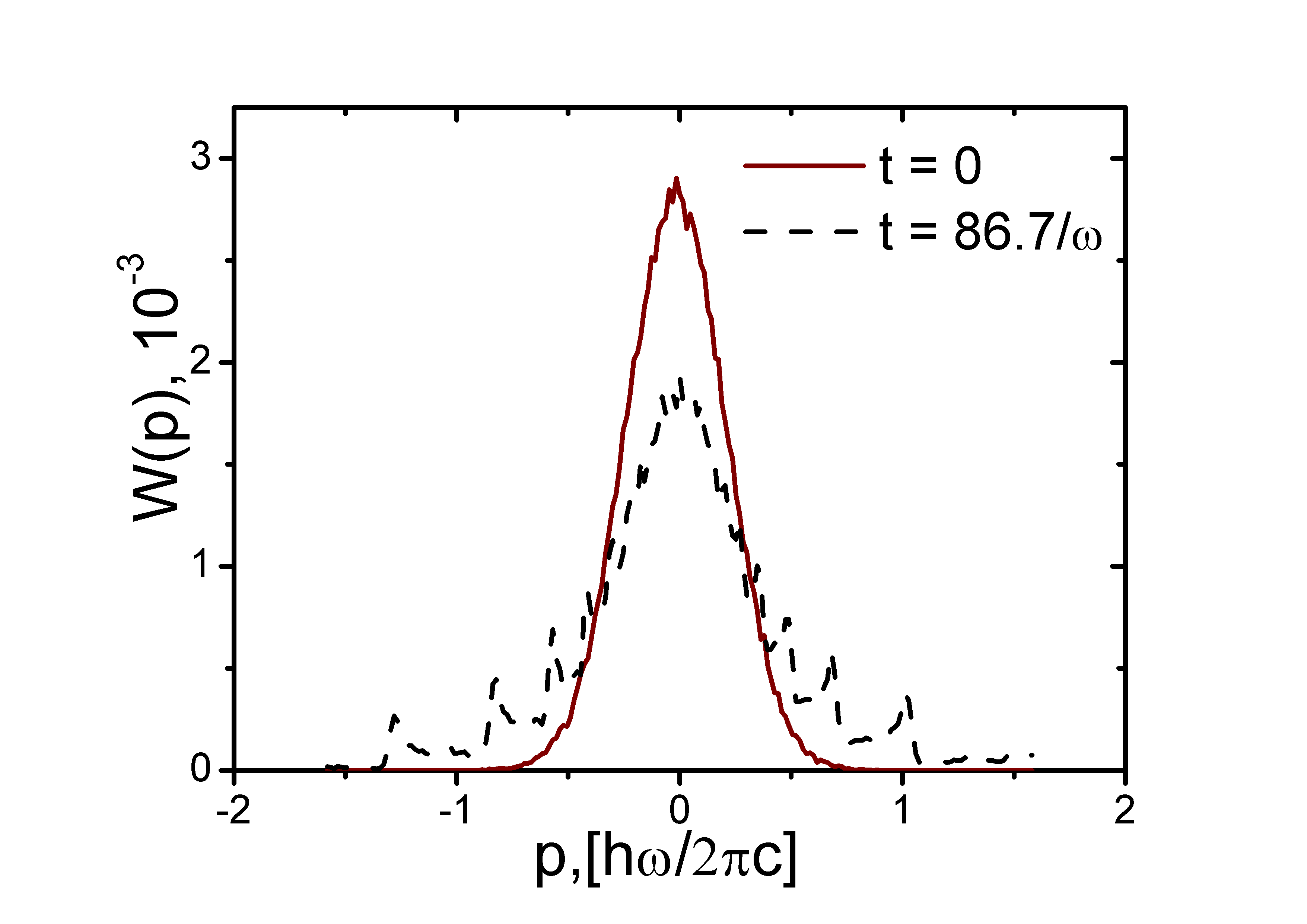
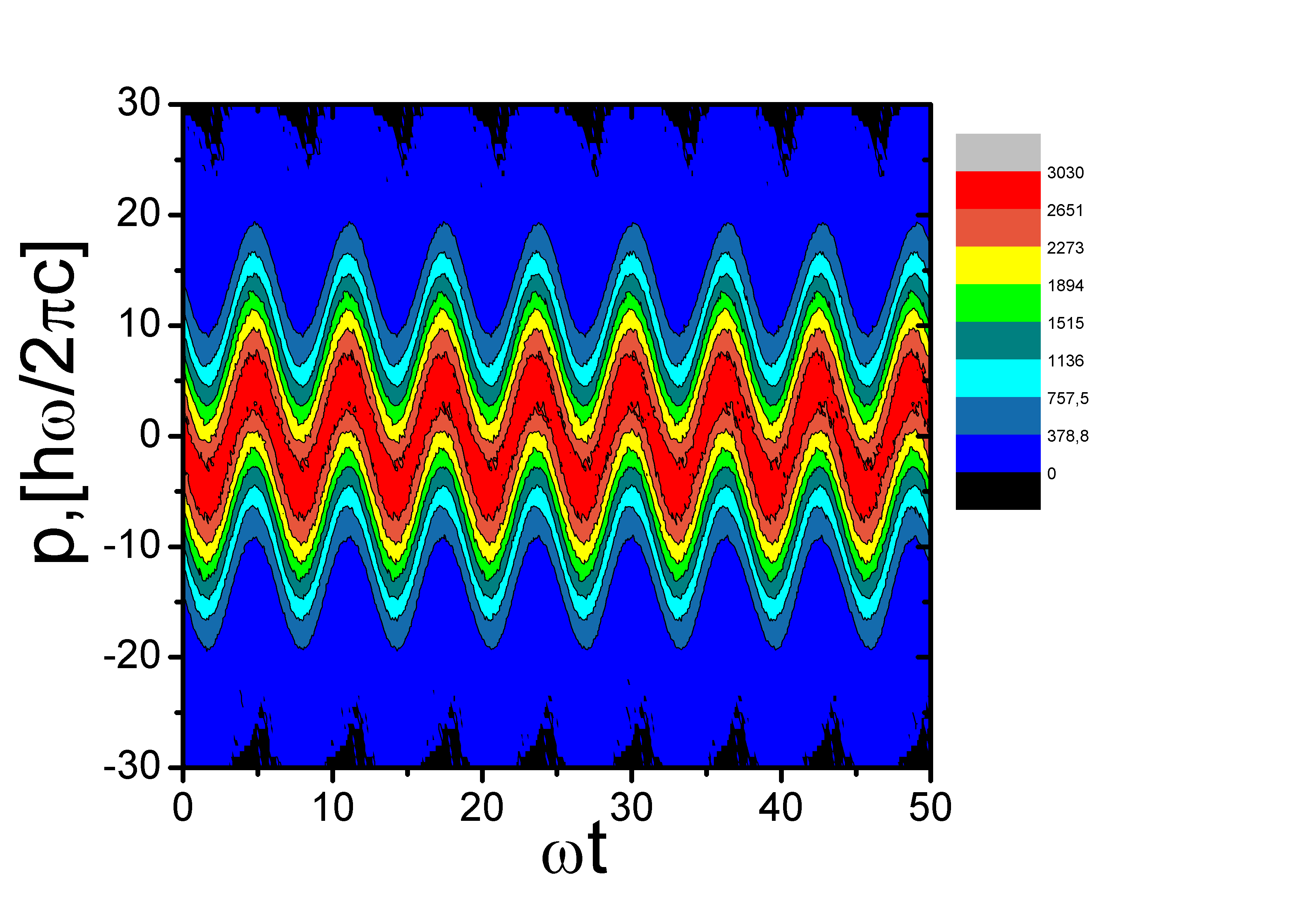
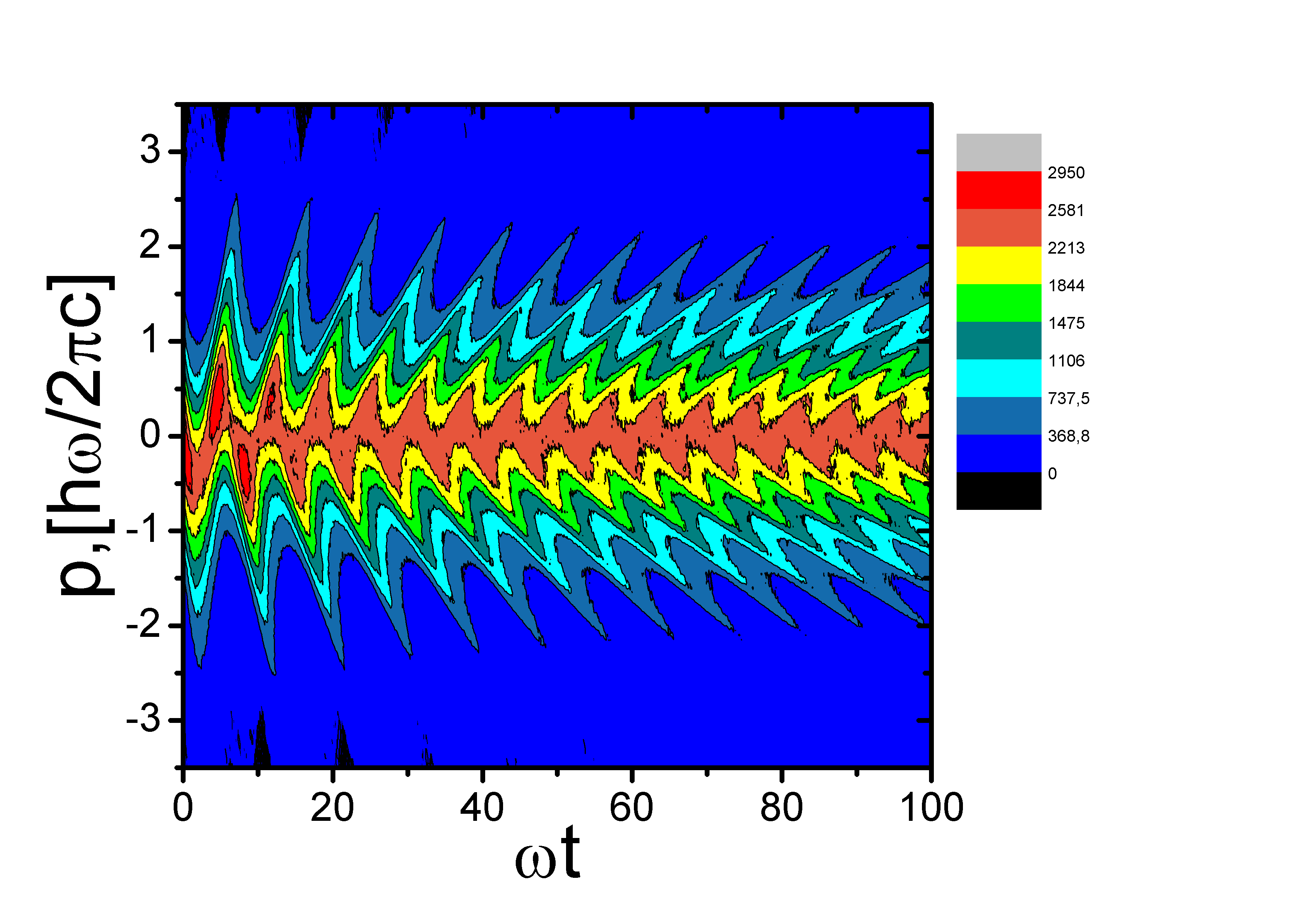
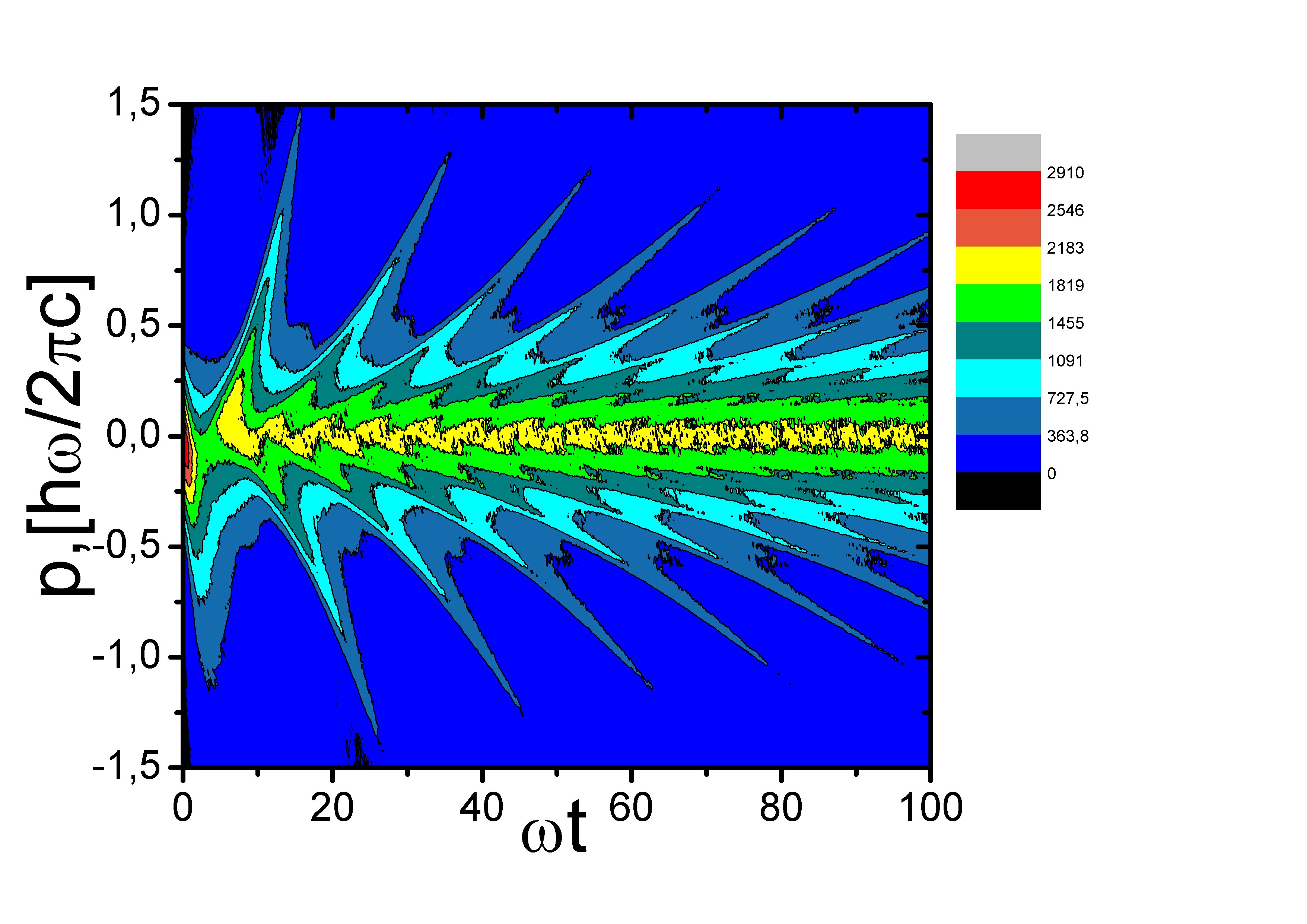
Figure 1: Time evolution of the non normalized momentum distributions for oscillators at $z=100$, $z=1$ and $z=0.1$. The left top panel – initial at $t=0$ (solid line) and at $\omega t=86.7$ distributions (dot line) for $z=0.1$ . The right top panel – the contour plot for $z=100$, the left bottom panel – the contour plot for $z=1$, the right bottom panel – the contour plot for $z=0.1$. Small oscillations on the initial distribution at $t=0$ characterize the error of the generated Gauss momentum distribution (21).

Velocity distribution $W(v)$ has an interesting shape presented by the Fig. 3 for oscillators with $z=1$ (top) and $z=0.1$ (bottom). Due to the complicated transformation $v=\frac{pc}{\sqrt{p^{2}+m^{2}c^{2}}}$ positions of the maximum of the velocity distributions $W(v)$ at initial time $t=0$ does not coincide with the position of the maximum of momentum distribution at $p=0$.

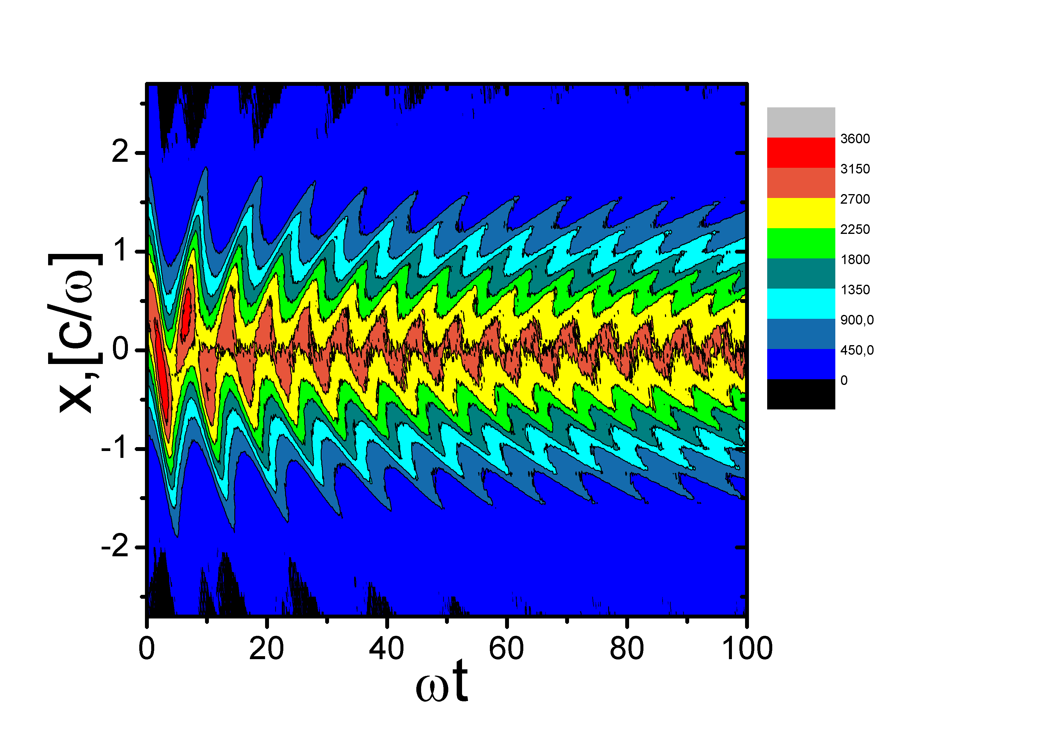
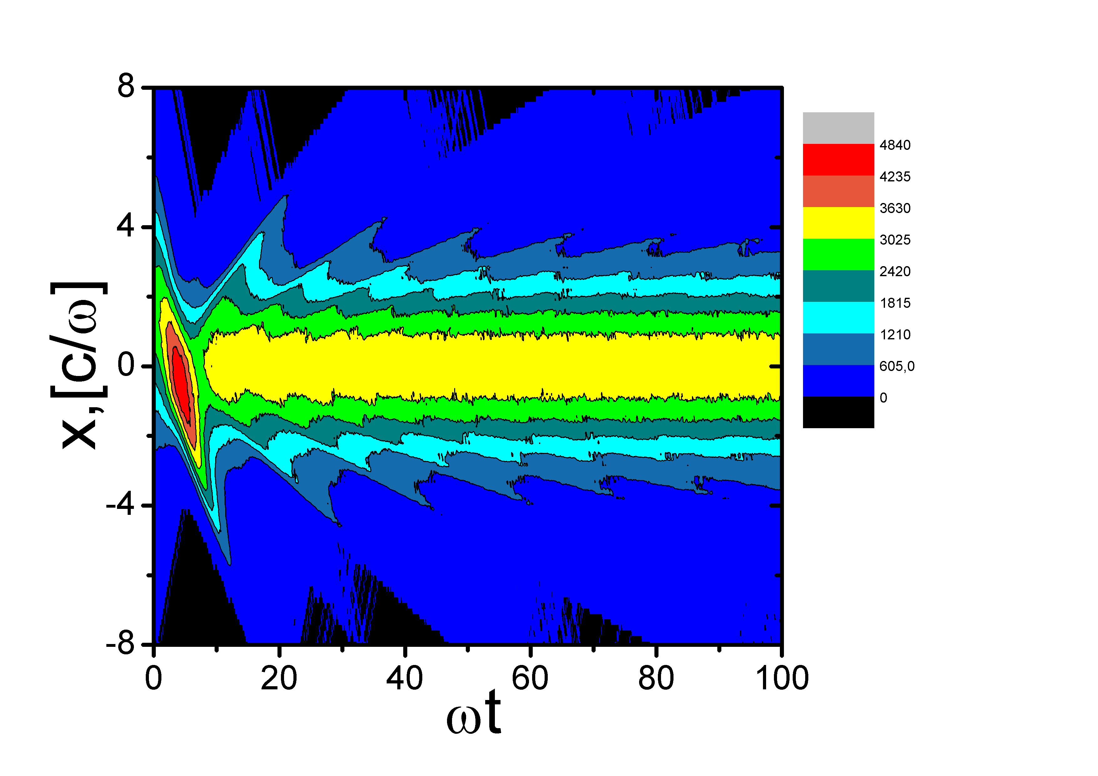
Figure 2: The time contour plot of the coordinate non normalized distributions. Left panel – $z=1$, right panel – $z=0.1$.

Moreover at time evolution the velocity distribution is restricted by the light speed velocity, while the momentum distributions has not any limits. Asymmetry of velocity distribution at the initial moment is the result of errors, which is related to sampling of the exponentially rare events in the tails of the momentum Gauss distributions function. Take notice that on Fig. 1 - Fig. 2 distributions are not normalized on unity. Its presented values show the number of the virtual trajectories have been counted in the vicinity of the each point on the plane related to presented distributions.

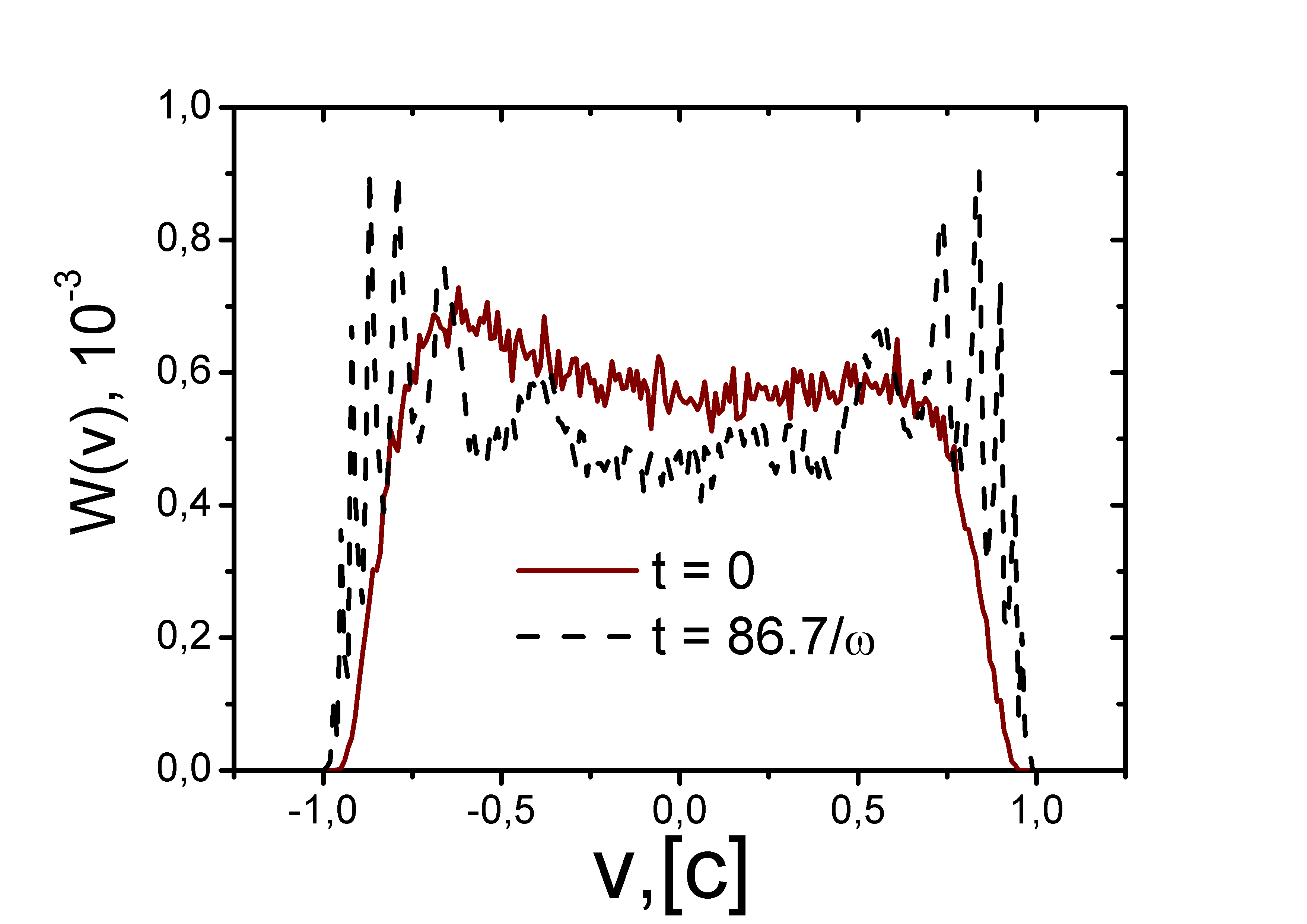
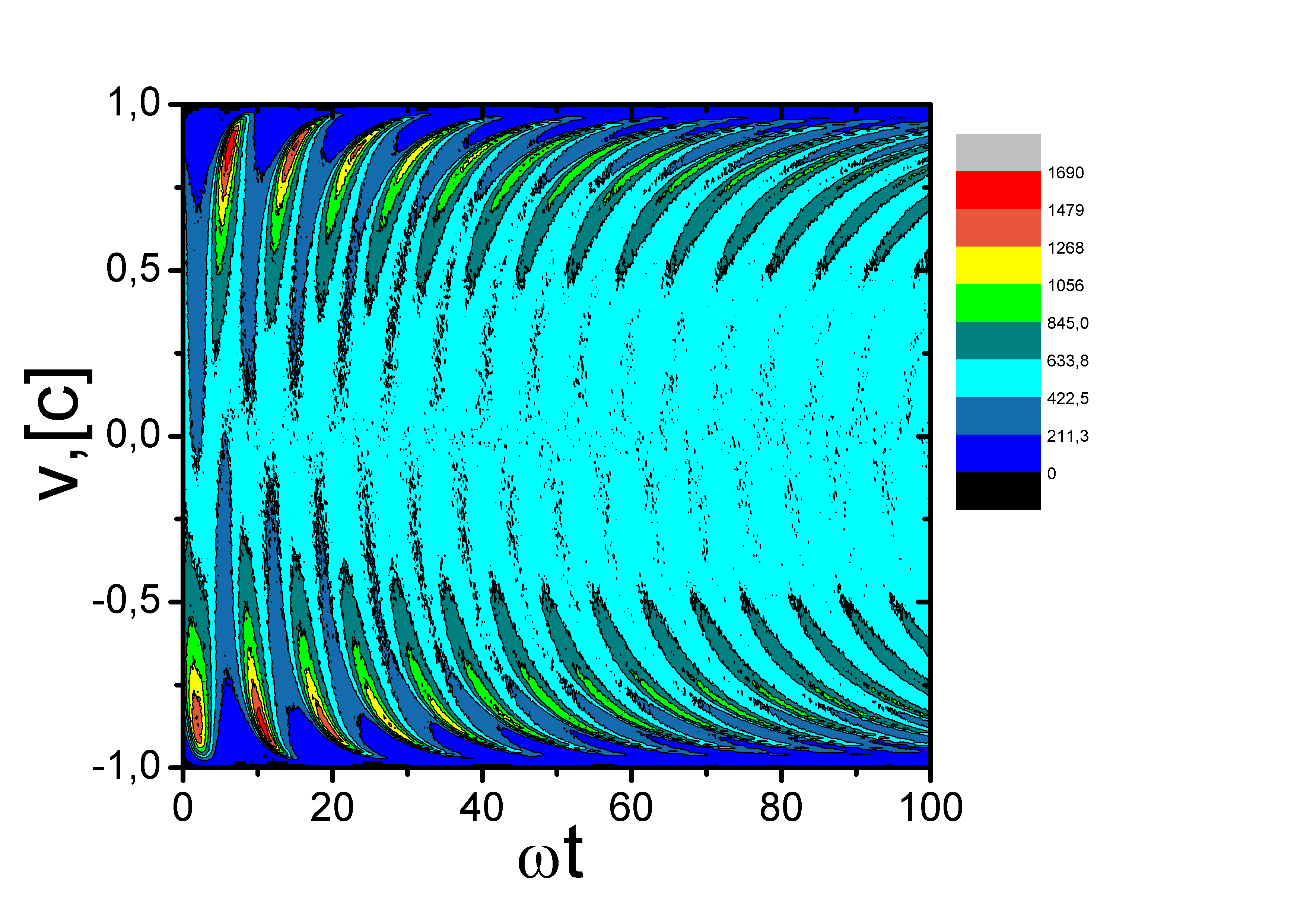
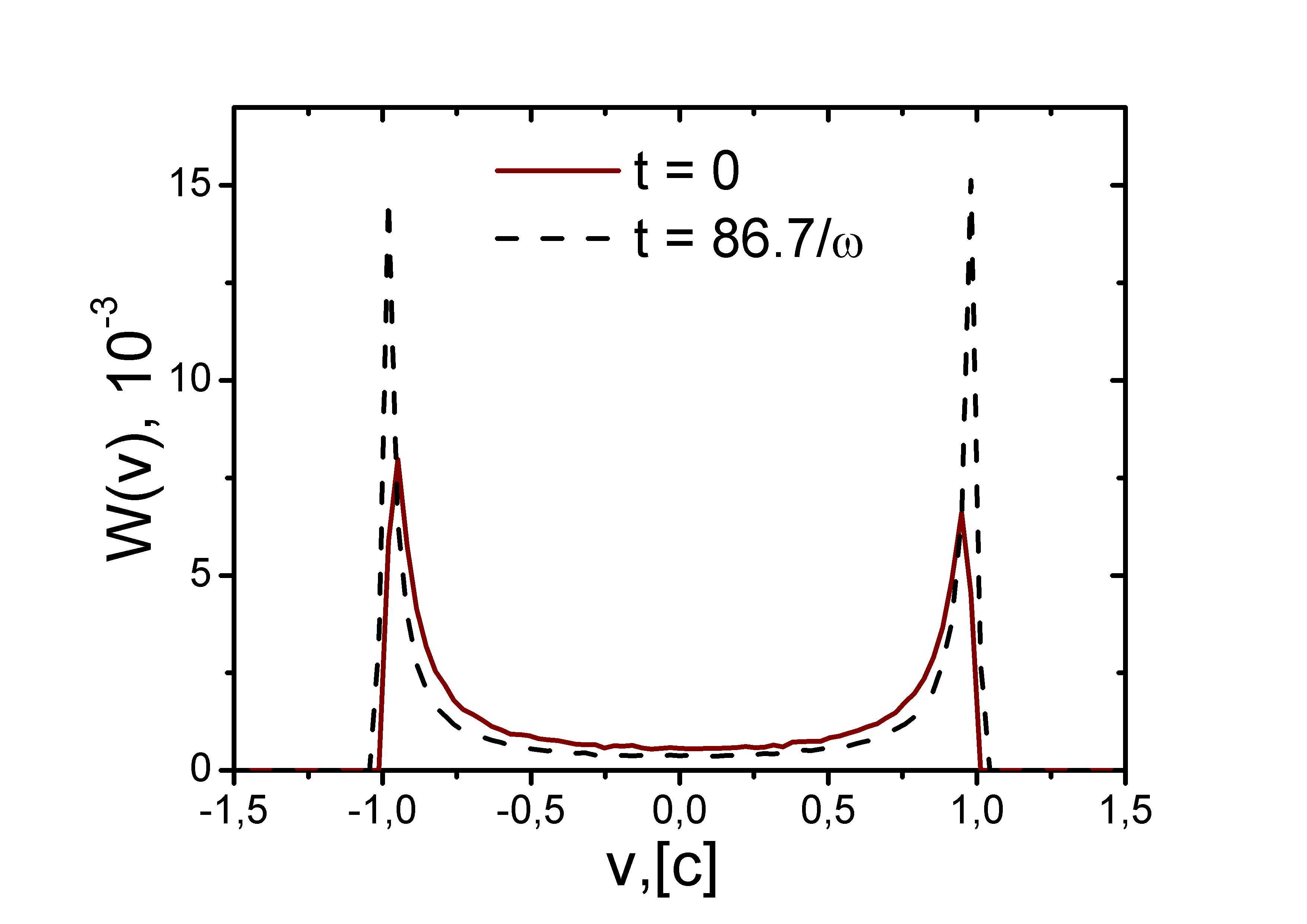
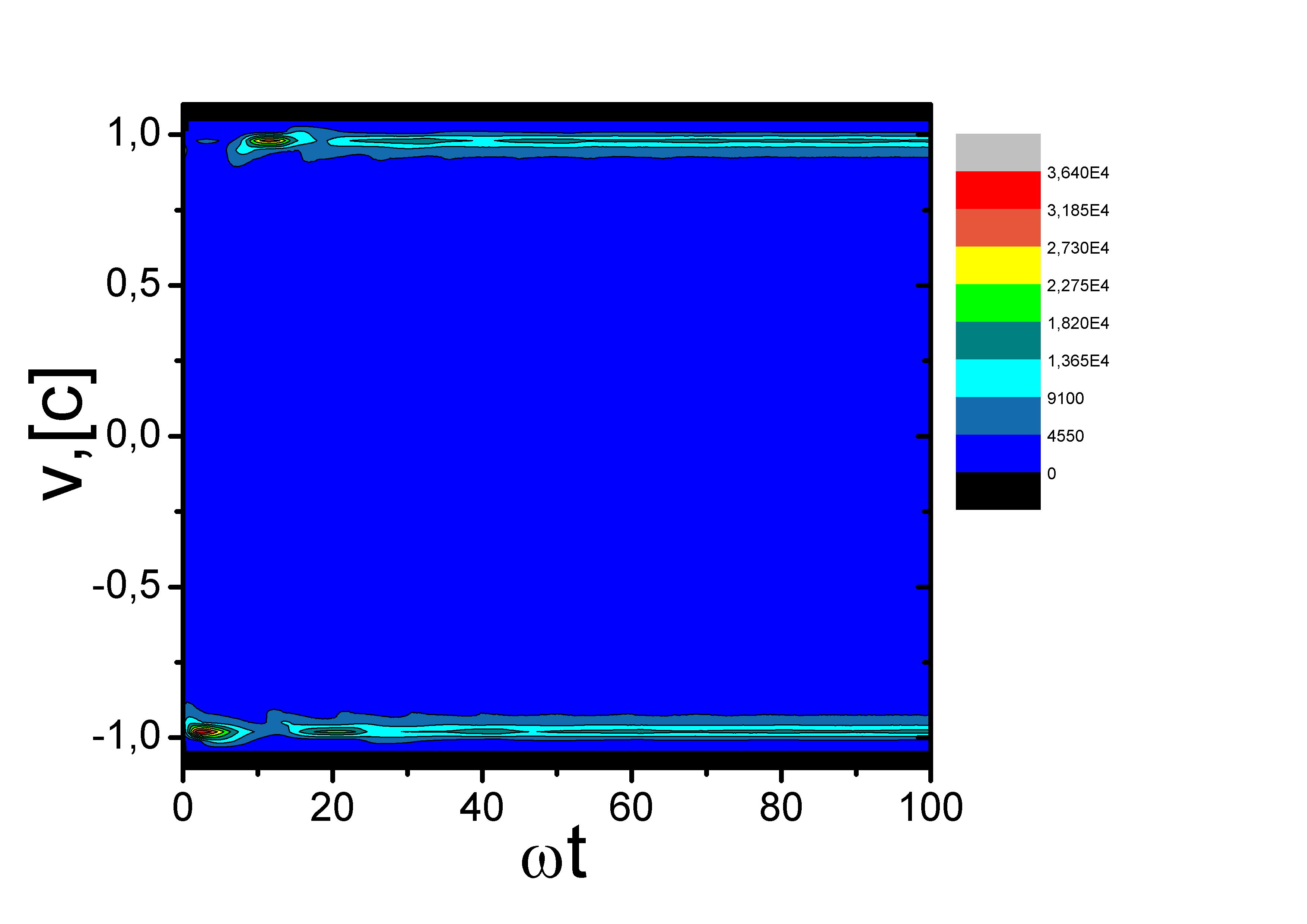
Figure 3: Time evolution of the non normalized velocity distributions for oscillators at $z=1$ (top) and $z=0.1$ (bottom). The left top panel – initial at $t=0$ (solid line) and at $\omega t=86.7$ distributions (dot line). The right top panel – the time contour plot, the left bottom panel – initial at $t=0$ (solid line) and at $\omega t=86.7$ distributions (dot line), the right bottom panel – the time contour plot

Average values of quantum operators. Now we are going to consider behavior of average values of quantum operators in time for discussed above initial Wigner function. On the Fig. 4 one can see time dependence of average momentum $<p(t)>$ and the average coordinate $<x(t)>$. For $z=100$ (weak relativism) $<p(t)>$ and $<x(t)>$ are sinusoidal functions with period of oscillation equal to $2\pi/\omega$. Here the average momentum and coordinate behave almost classically like sinusoidal trajectory corresponding to initial data $\tilde{p}(0)=0$, $\tilde{x}(0)=\tilde{x}_{0}$ quantum . To analyze the increasing influence of relativistic effects let us consider lines $2$,$3$,$4$. Firstly, with decreasing parameter $z$ period of oscillations is increasing. Secondly, oscillations are damped as the Wigner functions are spreading in the phase space.

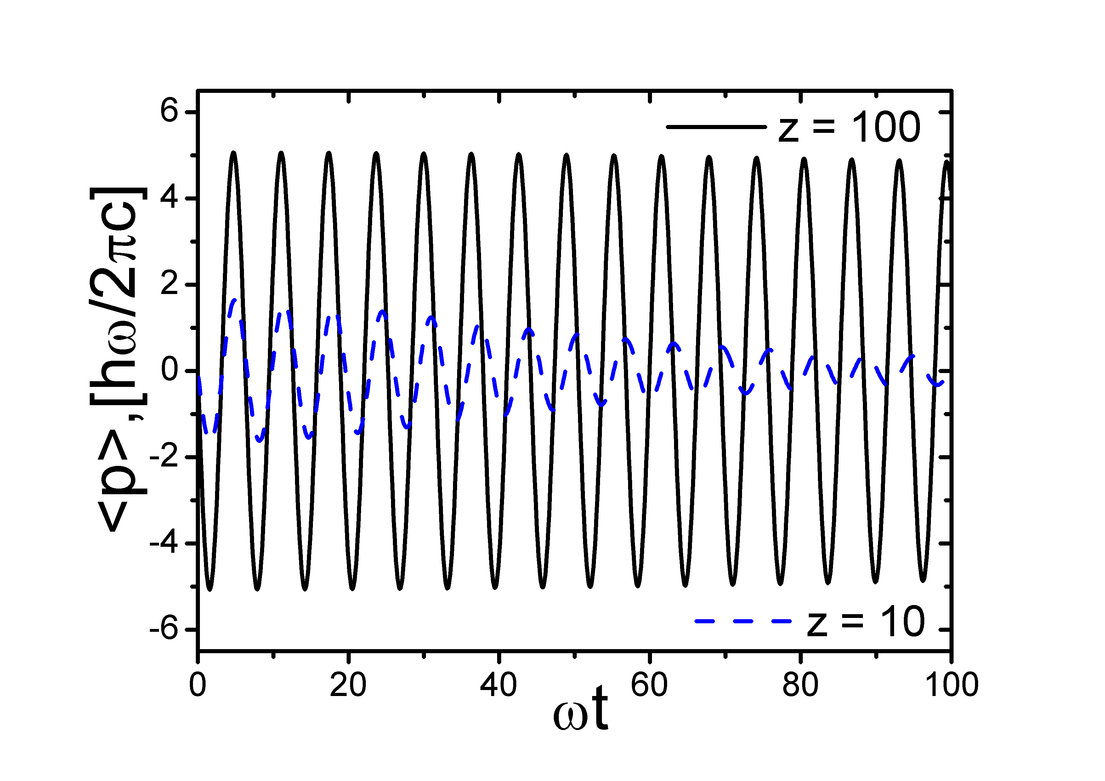
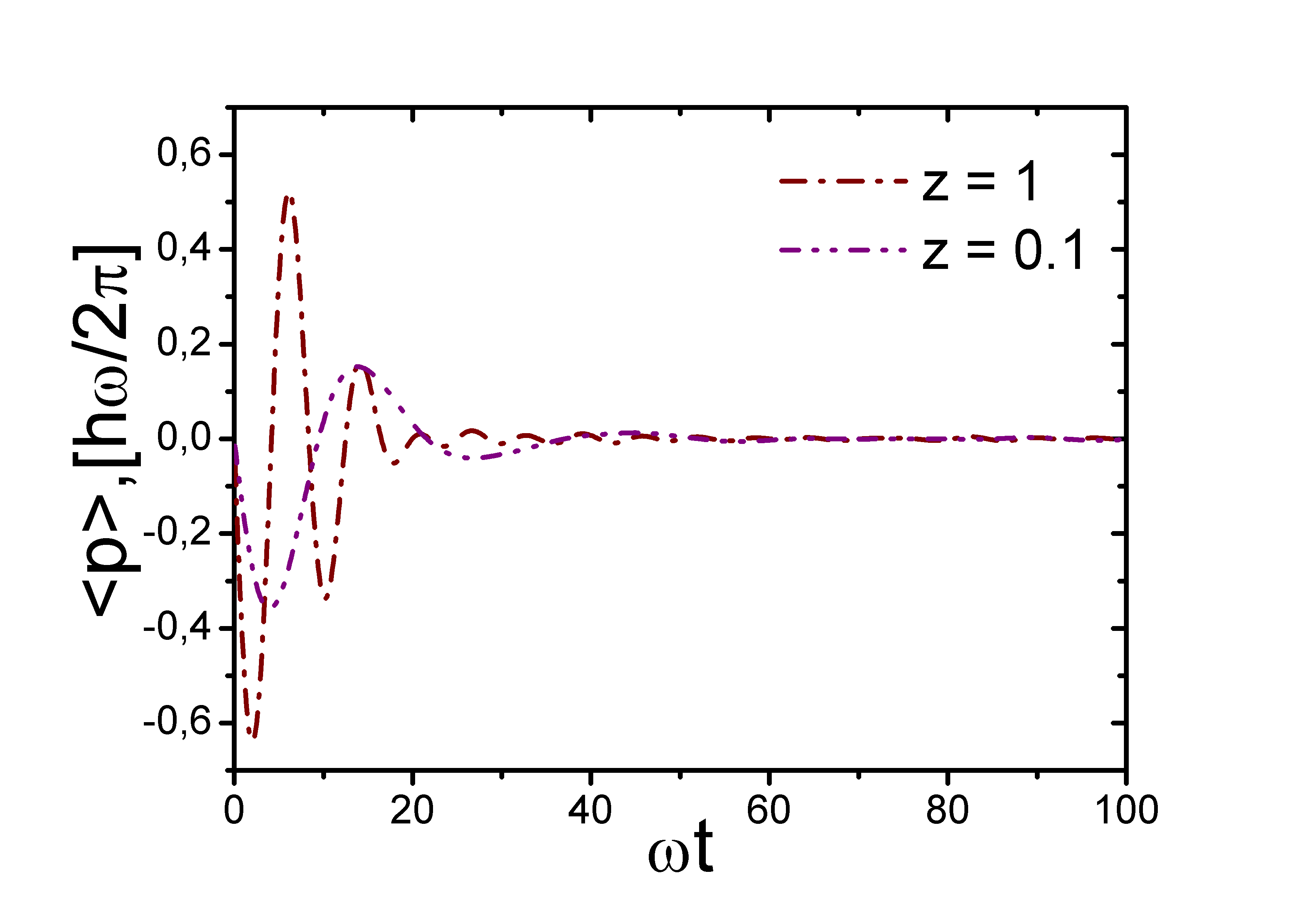
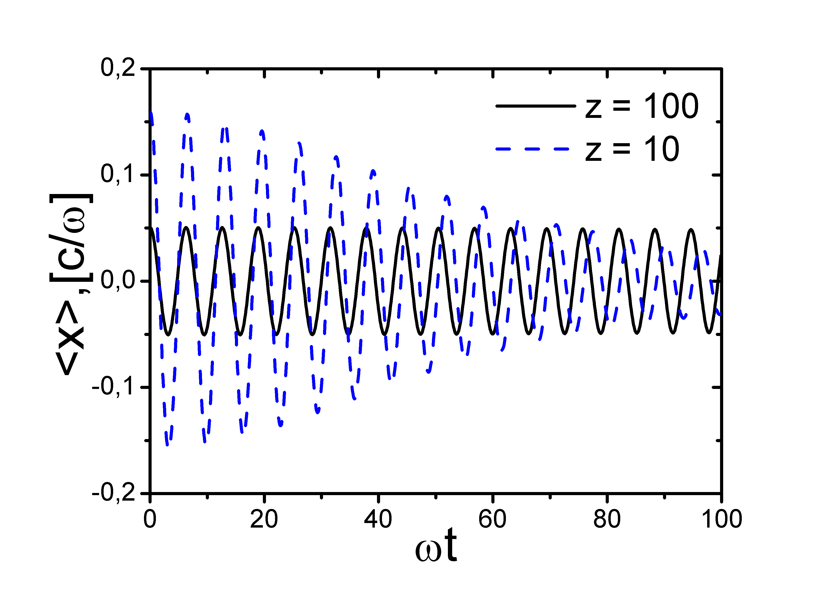
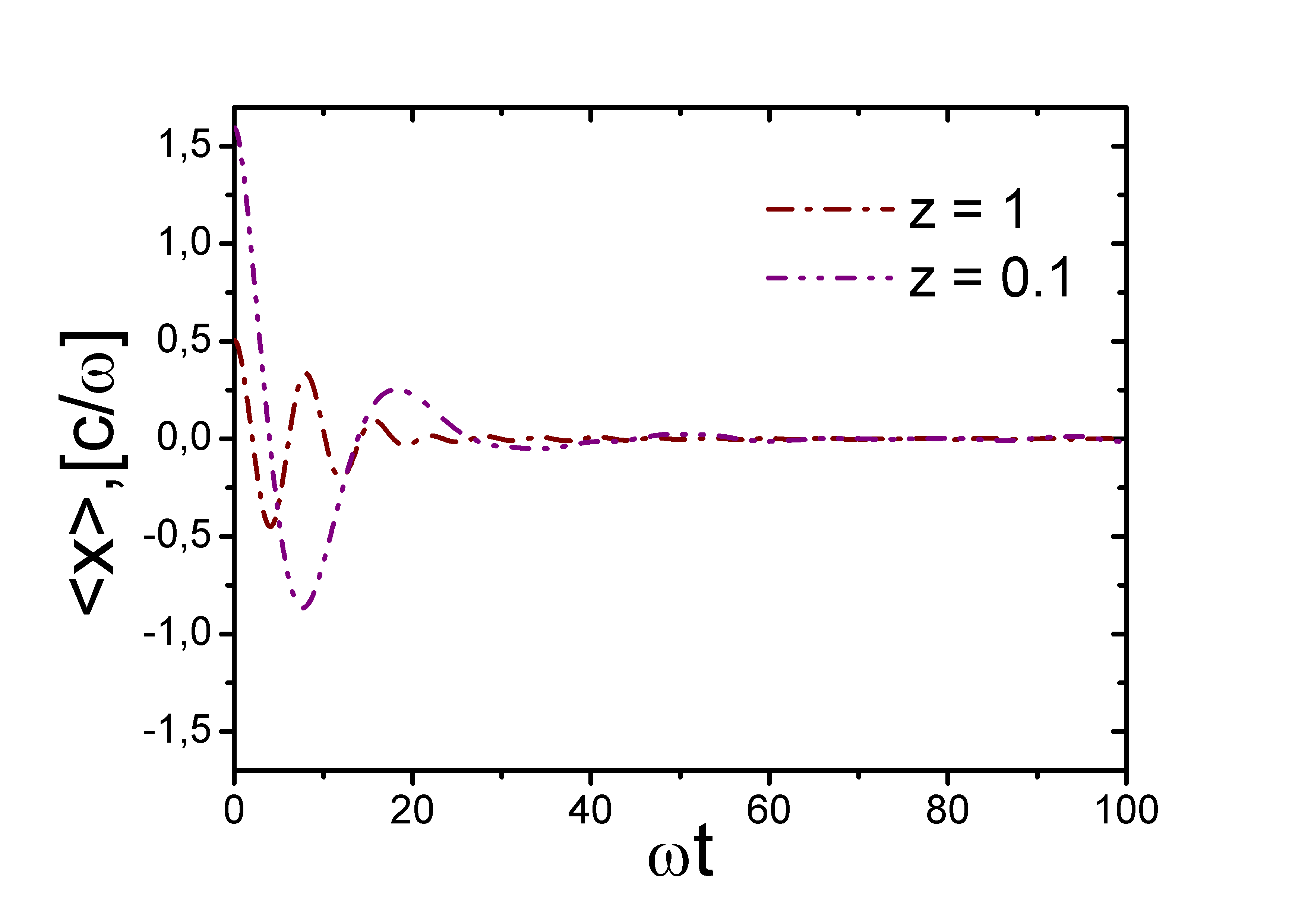
Figure 4: Dependence of average momentum $<p(t)>$ and average coordinate $<x(t)>$ on time. Lines $1$ correspond to oscillator with $z=100$, line $2$ - $z=10$, line $3$ - $z=1$ and line $4$ - $z=0.1$. With decreasing of z period of oscillations rises, while oscillations are damped.

Fig. 5 presents the time evolution of the average velocity $<v(t)>$. Behavior of the average velocity is similar to behavior of the average momentum and coordinate. Moreover, the phases of momentum and velocity oscillations (Fig. 4) coincide with each other. Let us stress that due to the influence of relativistic effects (lines $2,3,4$) $<p>/<v>$ is not equal to mass of oscillator $m$.

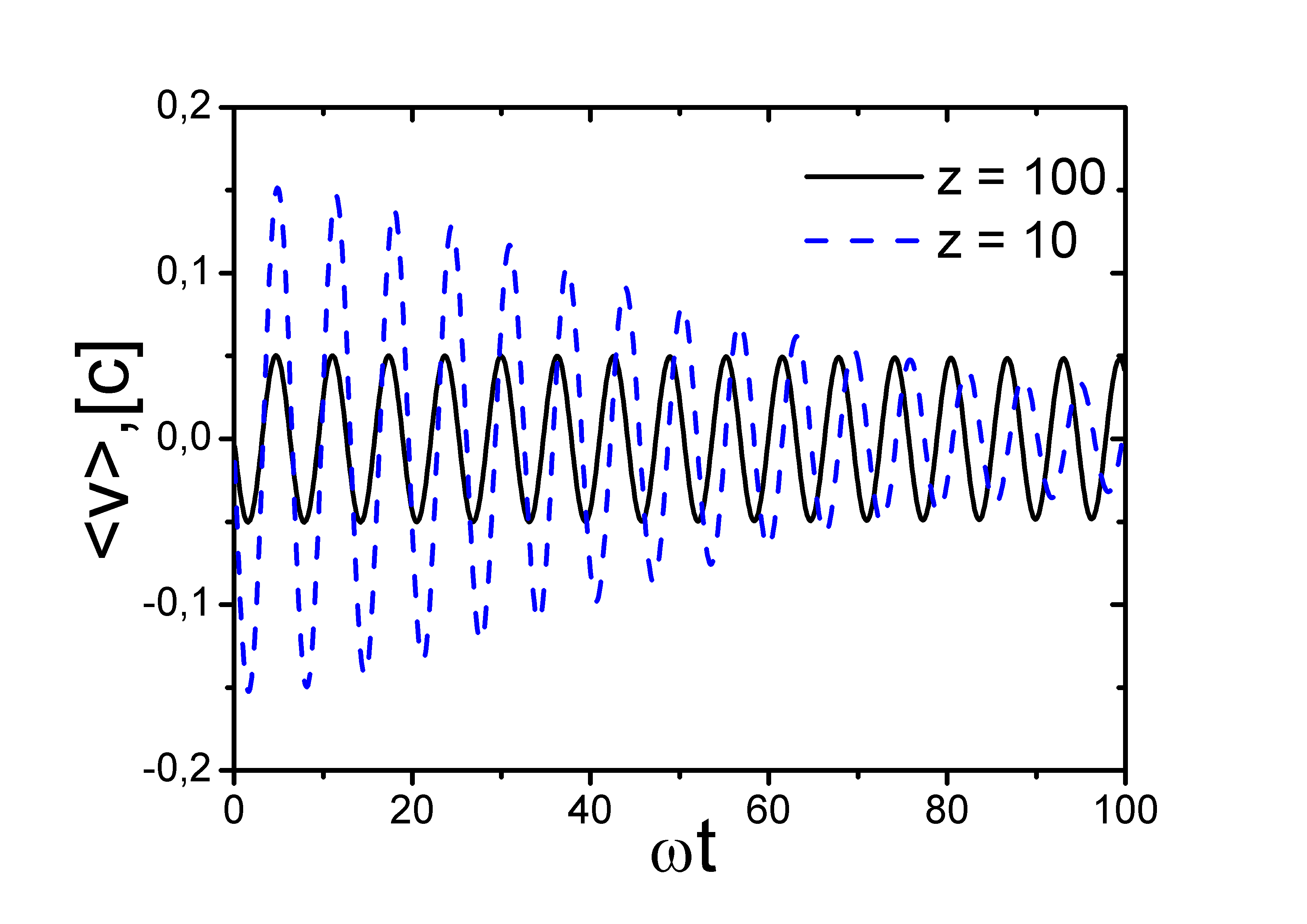
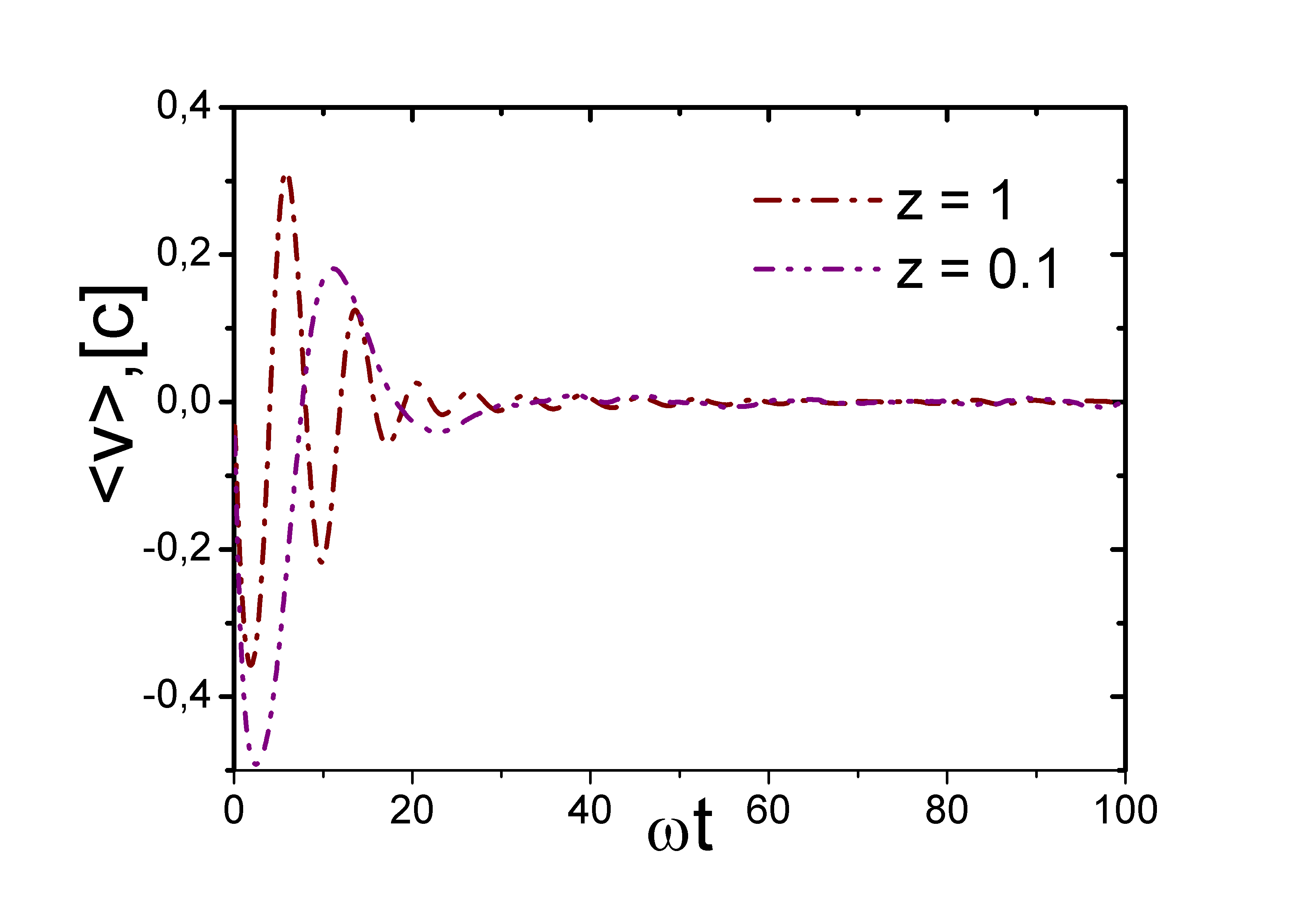
Figure 5: Dependence of average velocity $<v(t)>$ on time. Line $1$ corresponds to oscillator with $z=100$, line $2$ - $z=10$, line $3$ - $z=1$ and line $4$ - $z=0.1$.

The products of momentum and coordinate dispersions $<\delta p^{2}><\delta x^{2}>$ versus time are presented on the left panel of Fig. 6. The Heisenberg’s uncertainty principle is satisfied as $<\delta p^{2}><\delta x^{2}>\geq\hbar^{2}/4,$. More over these products have minimum at $t=0$ due to the proper choice of initial state. In case of weak relativism $z=100$ (line $1$) the product of dispersions is almost constant as the initial Wigner function is not spreading. This results to the horizontal line presenting the $<\delta p^{2}><\delta x^{2}>$. On the contrary the products of dispersions increase in time very fast for small $z$. The reason for this is that the initial Wigner function does not correspond to the coherent or eigen states of the semi-relativistic harmonic oscillator.

The right panel of Fig. 6 show the dependence of average energy $<E(t)>$ on time. As the considered oscillators are conservative the energies are constants. For weak relativism (lines $1$, $2$) average energy $<E>$ is circa the rest energy $mc^{2}$ ($100\hbar\omega$ and $10\hbar\omega$ ). Due to the strong relativistic effects (line $4$) the average energy $<E>$ is considerably greater then rest energy $mc^{2}$ ($mc^{2}=0.1\hbar\omega$ for $z=0.1$).

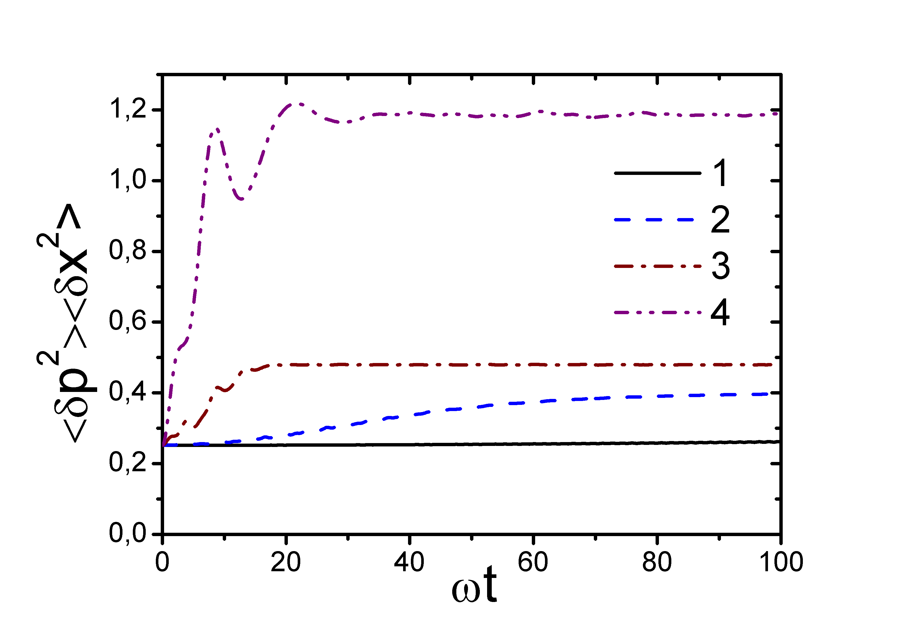
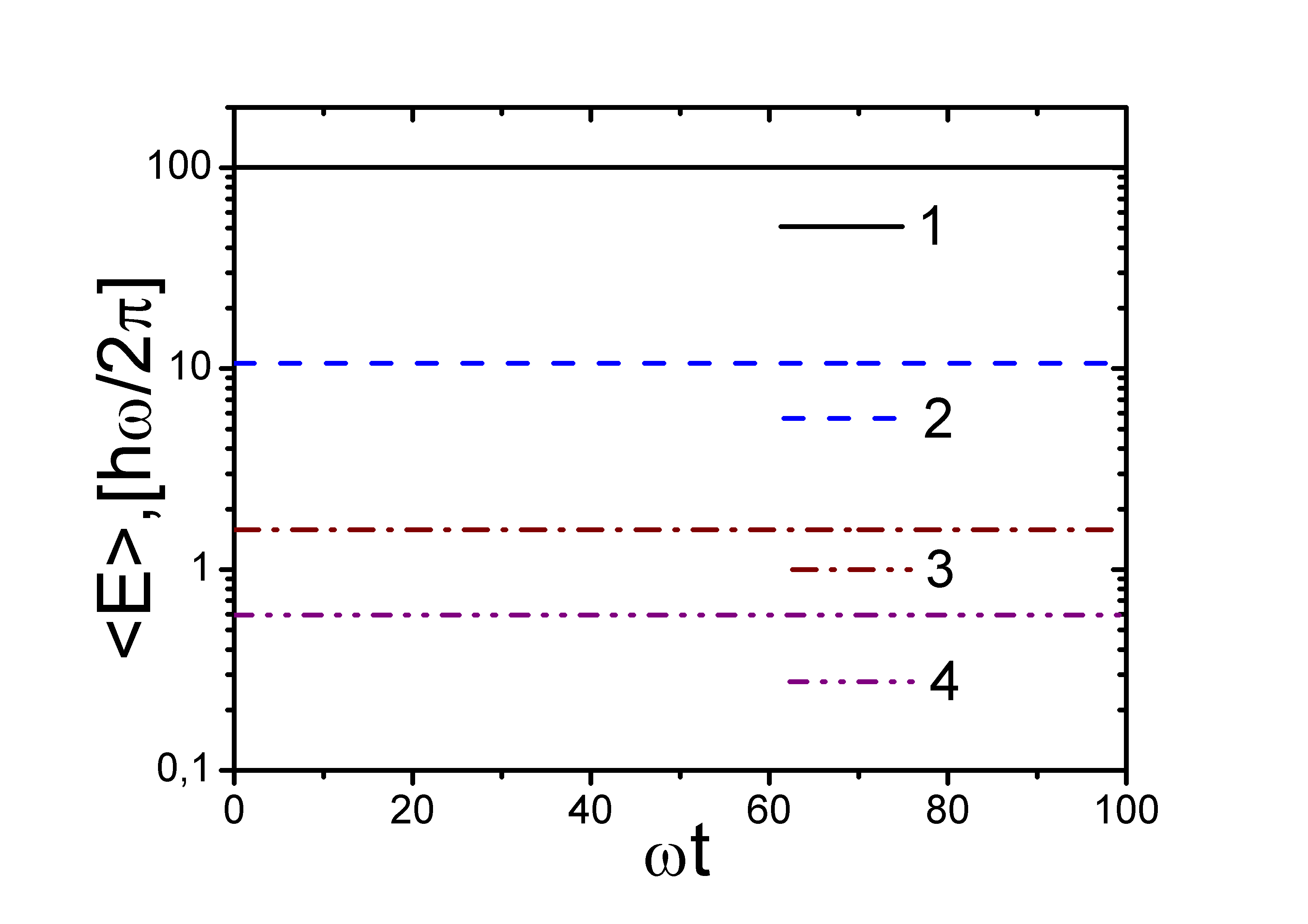
Figure 6: Left panel – dependences on time of the products of the momentum and coordinate dispersions. Right panel – dependence of average energy $<E>$ on time for semi-relativistic oscillators.

Virtual trajectories. To understand physical reasons of the different properties of non-relativistic and relativistic harmonic oscillators we have to consider behavior of individual virtual trajectories related to initial delta distribution with fixed initial momentum and coordinate

$$W_{0}(x_{0},p_{0};0)=\delta(x-x_{0})\delta(p-p_{0}),$$ (23)

where $(p_{0},x_{0})$ are initial condition of the virtual trajectories. Here due to the limitation (9) distribution $W_{0}$ can not be considered as physical Wigner function. However this choice of the Wigner function can help in understanding peculiarities in the time behavior of the discussed above average values. The given choice of the Wigner function (23) reduces the averaging over ensemble of the virtual trajectories to the consideration of the contribution only one virtual trajectory with fixed initial $x_{0},p_{0}=0$ like in classical case.

Fig. 7 presents the virtual trajectories as function of time. For $z=100$ non-relativistic trajectories look like sinusoid curves with equal oscillation periods (trajectories $1$, $2$ on the left panel). Let us note that energy of the virtual trajectory is proportional to the square of $x_{0}$ and in the relativistic case (central and right panels $z=0.1$) oscillation period strongly increases with growth of the energy of trajectory (see (19)). Period of oscillations of $x(\omega t)$ for curve $4$ is longer than for one $3$ due to the larger value of energy. Moreover, curves $3$ and $4$ tend to become the zig - zag lines.

Velocity of the trajectory $4$ (right panel of the Fig. 7) looks like rectangular wave for high energy. This figure illustrates that mostly the virtual trajectory has velocity $v$ approaching the velocity of light $c$ and only near the turning points $v$ differs from this limit. Velocity of trajectory $3$ for the same $z$ but lower energy differs considerably from rectangular wave.

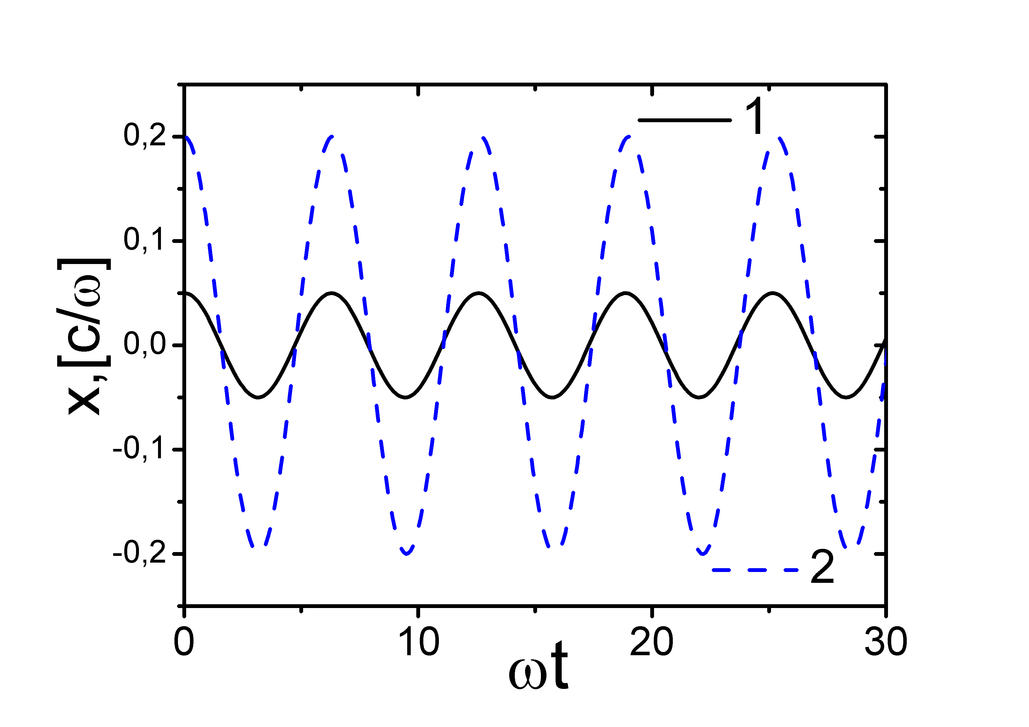
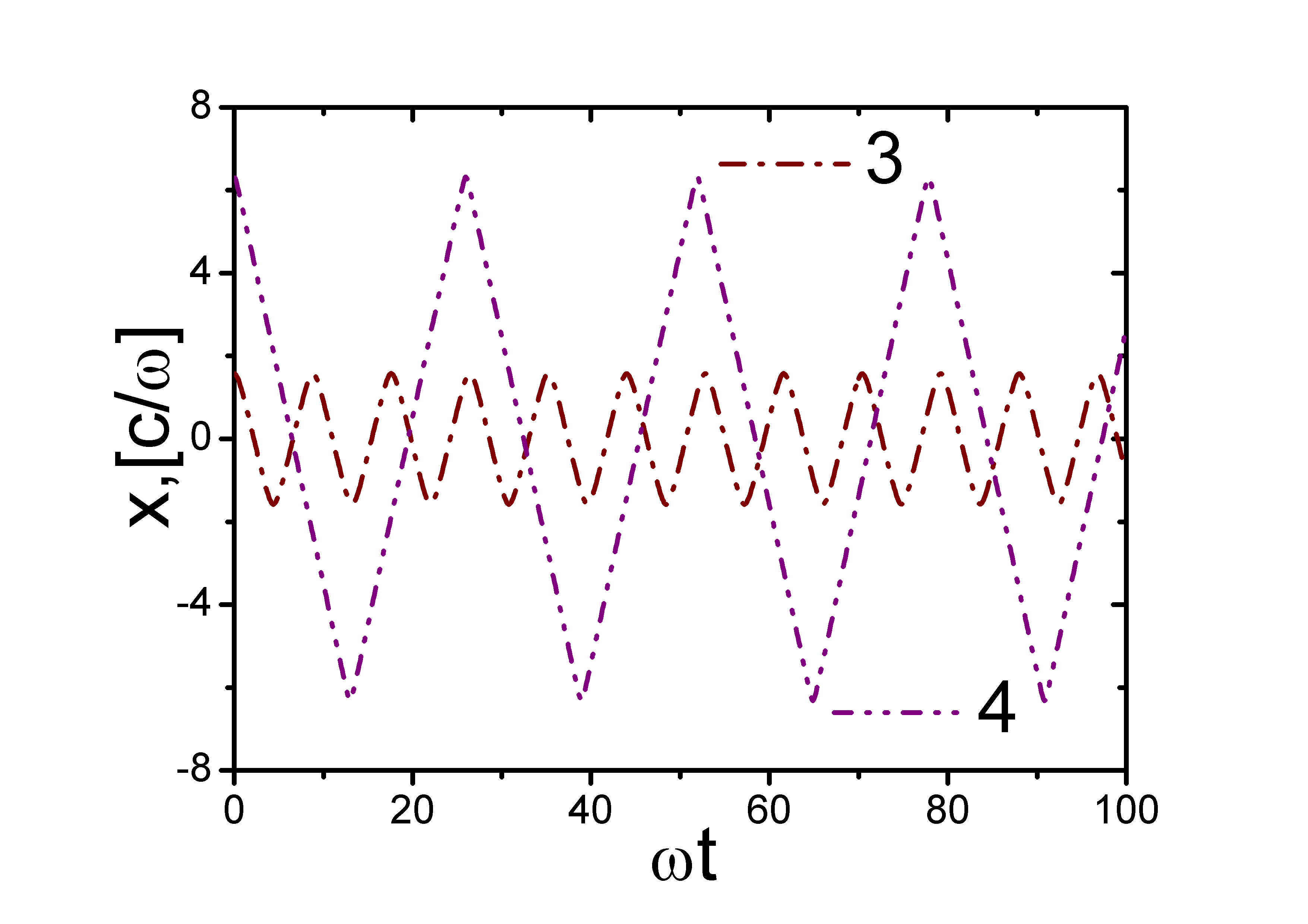
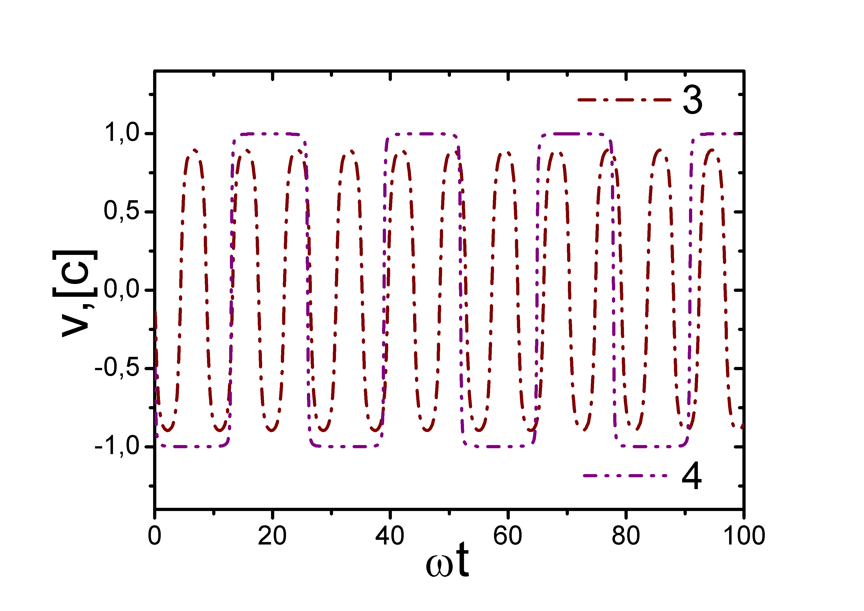
Figure 7: Virtual trajectories for $p_{0}=0$. Left panel - non-relativistic trajectories $1$ (with $x_{0}=0.05c/\omega$) and $2$ (with $x_{0}=0.2c/\omega$) for $z=100$. Central and right panels - relativistic trajectories $3$ (with $x_{0}=1.58c/\omega$) and $4$ (with $x_{0}=6.3c/\omega$) $z=0.1$.

Left and cetral panels of the Fig. 8 show non-relativistic momentum virtual trajectory versus time for $z=100$ (lines $1,2$) and relativistic trajectories for $z=0.1$ (lines $3,4$). The time dependences of $p(\omega t)$ look practically as sinusoid curves. In the left panel period of momentum oscillations for trajectories $1$ and $2$ is almost the same. In the central panel oscillation period is longer for the relativistic trajectory $4$ with higher energy.

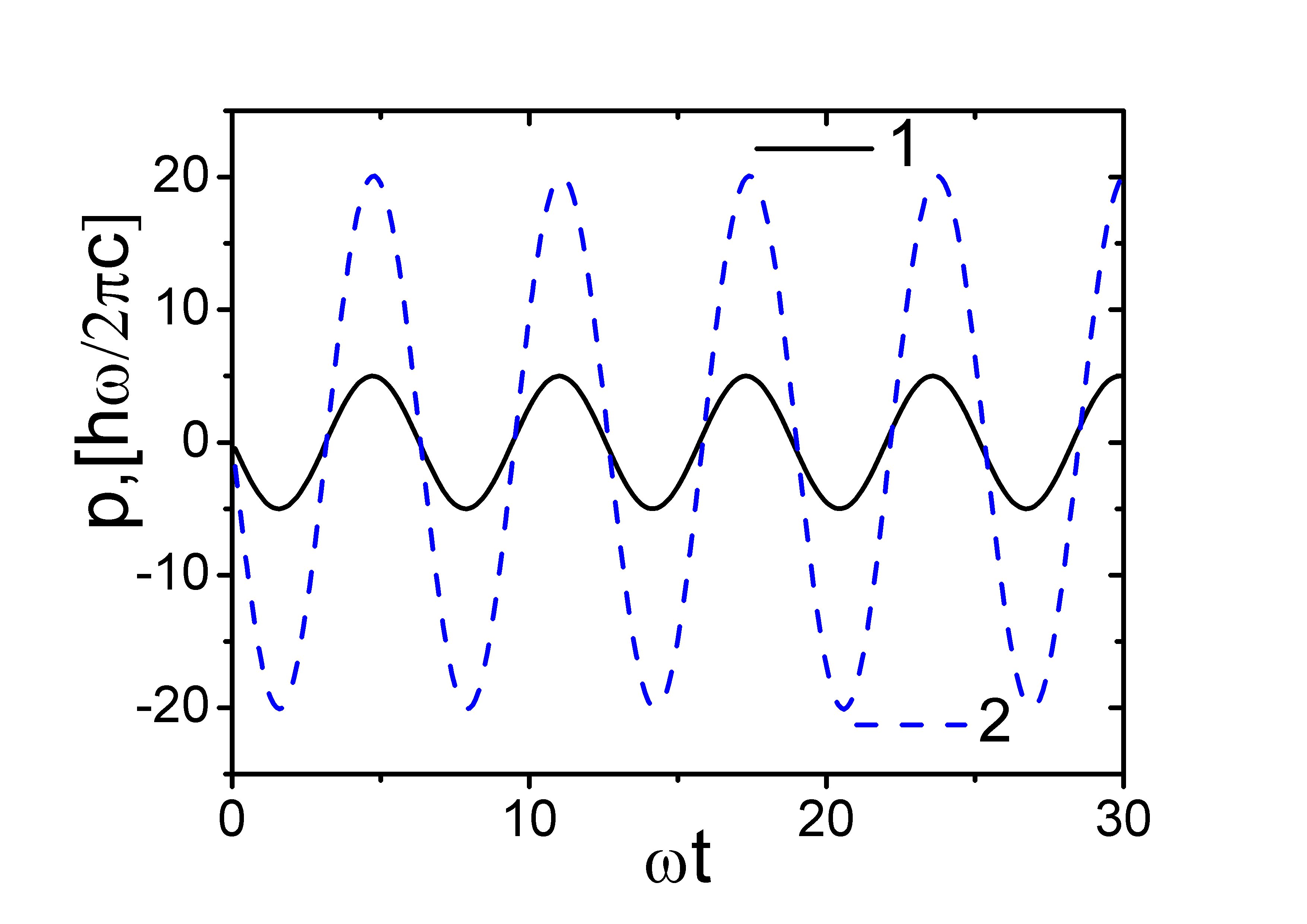
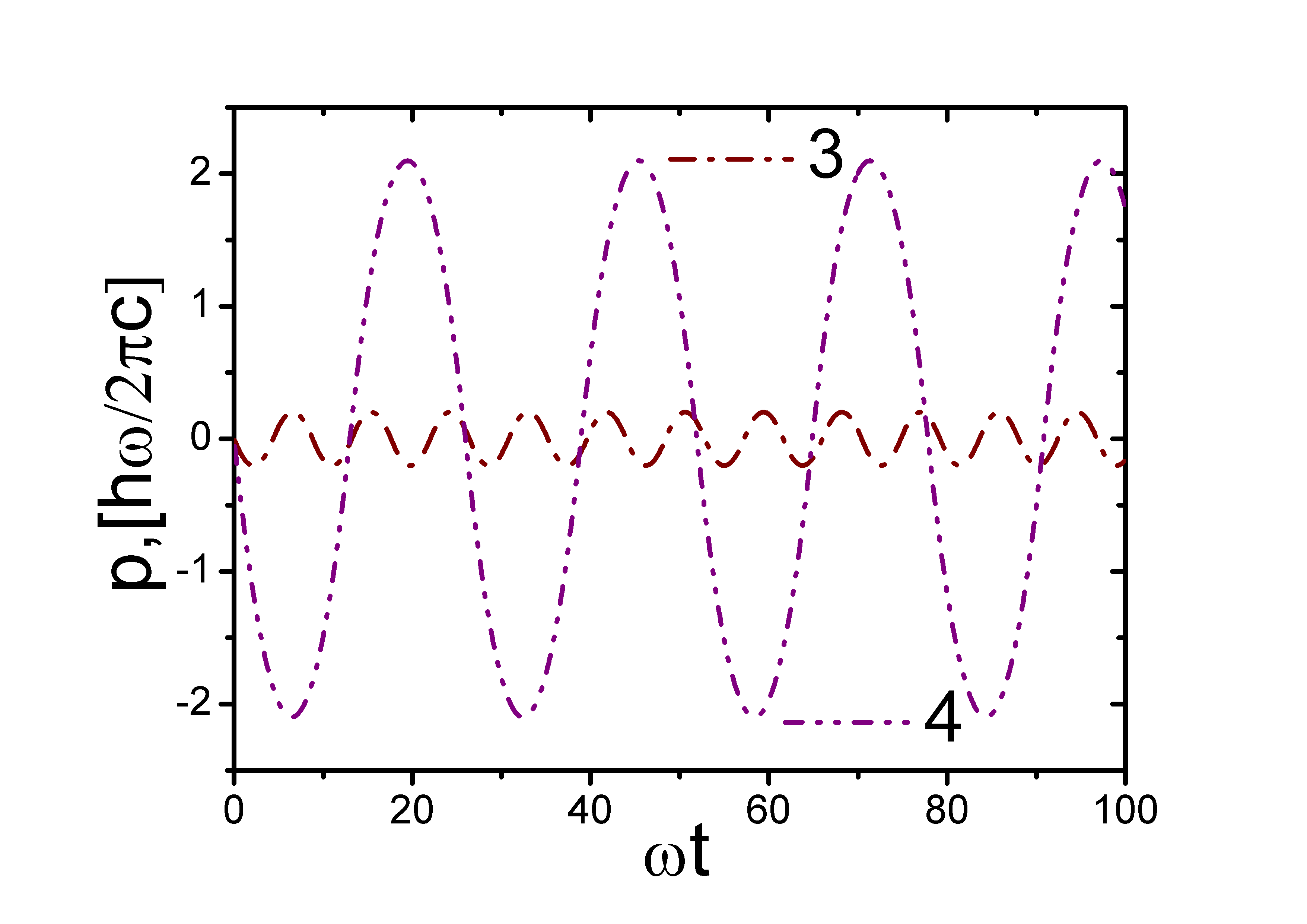
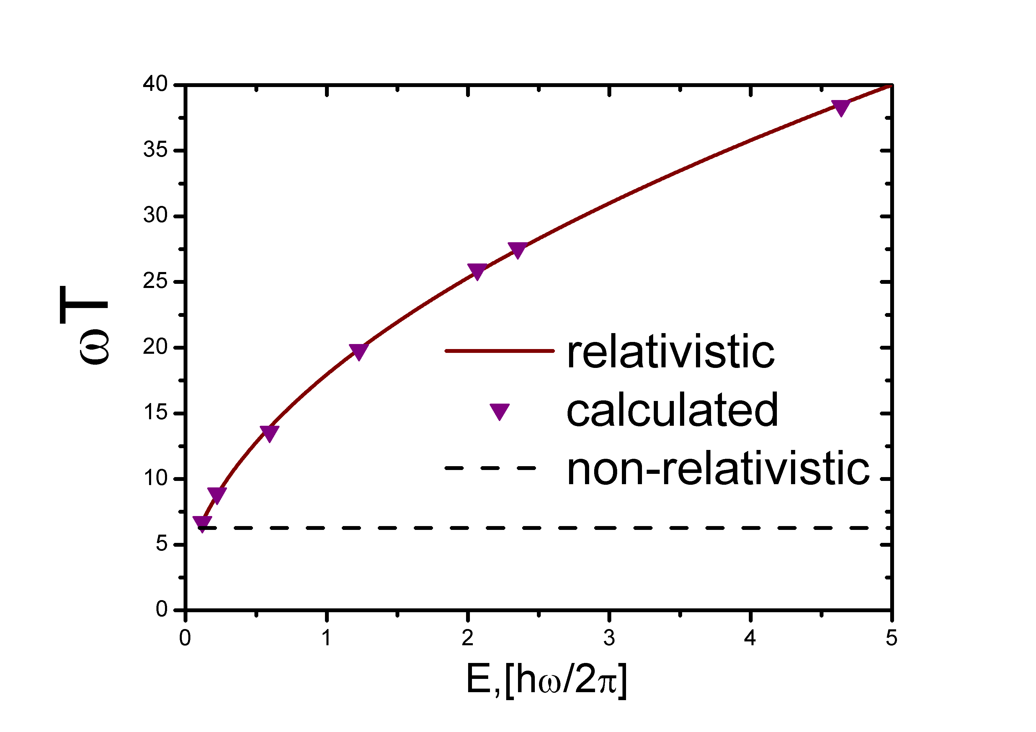
Figure 8: Virtual trajectories for $p_{0}=0$. Left panel - non relativistic trajectories $1$, $2$, central panel - relativistic ones $3$ and $4$. Oscillation period of relativistic trajectory $4$ is longer than $3$ due to the larger value of virtual energy. Right panel - period of oscillations of the virtual trajectories versus energy for $z=0.1$. Solid line - formula (19), triangles - results of numerical simulations, dashed line - non-relativistic case.

Comparison of analytical and numerical calculations of the oscillation period is presented by the right panel of the Fig. 8. Analytical dependence of oscillation period on energy according to the formula (19) is plotted by solid curve for $z=0.1$. Results of numerical calculations presented by triangles agree very well with analytical dependence.

Time dilation. One of the most important relativistic effects is the time dilation: proper time of relativistic particle is slower than time in the non -relativistic lab frame of reference (inertial). Now we will consider this effect for semi-relativistic harmonic oscillator. We begin our consideration for one virtual trajectory $p(t),x(t)$.The relationship between proper time and lab time is well known for the case, when particle moves with constant velocity:

$$t^{\prime}-t^{\prime}_{0}=(t-t_{0})\sqrt{1-\frac{\dot{x}(t)^{2}}{c^{2}}},$$ (24)

where $\dot{x}(t)$ is velocity of the particle, $t-t_{0}$ is time interval between two events in lab frame of reference, $t^{\prime}-t^{\prime}_{0}$ is time interval between this two events in the rest frame of particle. In case of oscillator, however, particle’s velocity is not a constant and formula (24) is right only for infinitesimal time intervals:

$$dt^{\prime}=dt\sqrt{1-\frac{\dot{x}(t)^{2}}{c^{2}}}\quad\mbox{while for finite time interval }\quad t^{\prime}-t^{\prime}_{0}=\int\limits_{t_{0}}^{t}{dt}{\sqrt{1-\frac{\dot{x}(t)^{2}}{c^{2}}}}.$$ (25)

Dependence on time for virtual trajectories with different energies is represented in logarithmic scale by the left panel of Fig. 9 for $z=0.1$. Almost constant parts of the curves ((4),(5)) related to the trajectories with high energy and correspond to the motion with velocity of order of the speed of light $c$.

In case of semi-relativistic oscillator with Hamiltonian (15) one has to average integral in (25) over all virtual trajectories. So for quantum oscillator described by the Wigner function $W(x,p;t)$ the time dilation for semi-relativistic oscillator can be calculated by formula:

$$t^{\prime}-t^{\prime}_{0}=\int\limits_{t_{0}}^{t}{dt}\int{W(x,p;t)\frac{1}{\sqrt{1+(p/mc)^{2}}}}{dp}{dx}\quad\mbox{related to the 'time dilation operator'- }\quad d\hat{t}^{\prime}=dt\sqrt{1-\frac{\hat{\dot{x}}(t)^{2}}{c^{2}}}.$$ (26)

In numerical calculation the averaging has been done over all virtual trajectories for each time moment $t$. Results are represented by the right panel of the Fig. 9 for oscillators with $z=100$, $10$,$1$ and $0.1$.

Figure 9: Time dilation for $t_{0}=0$. Left panel - the time dilation for virtual trajectories with $z=0.1$. Energies $E_{tr}$ of the virtual trajectories: $1$ - $0.1\hbar\omega$ (resting particle); $2$ - $0.13125\hbar\omega$; $3$ - $0.225\hbar\omega$; $4$ - $0.6\hbar\omega$; $5$ - $2.1\hbar\omega$. Right panel - the time dilation for quantum semi-relativistic oscillators.

IV Conclusion

In this paper we are doing the exact simulation of time evolution of semi-relativistic quantum 1D harmonic oscillator. To solve the Wigner - Liouwille equation for such system we combine Monte-Carlo procedure and molecular dynamics methods. As initial Wigner quasi distribution function we have used a coherent state of appropriate non relativistic harmonic oscillator. We have studied the time evolution of the momentum, velocity and coordinate Wigner distributions and average values of quantum operators. Obtained results demonstrates, that relativistic treatment results in the appearance of the new physical effects as opposed to non-relativistic case. Interesting is the complete changing of the shape of the momentum, velocity and coordinate distribution functions as well as formation of "unexpected protuberances". We have also calculated relativistic time dilation for oscillator, as it can be useful for consideration of the life -time of the particle bound states in the traps.

References

- (1) M. Moshinsky, The Harmonic Oscillator in Modern Physics: from Atoms to Quarks (New-York: Gordon and Breach), (1969).
- (2) R. P. Feynman, and A. R. Hibbs, Quantum Mechanics and Path Integrals (McGraw-Hill, New York), (1965).
- (3) V. Tatarskii, Sov. Phys. Uspekhi 26, 311 (1983).
- (4) E. E. Salpeter and H. A. Bethe, Phys. Rev. 84, 1232, (1951).
- (5) E. E. Salpeter, Phys. Rev. 87, 328, (1952).
- (6) W. Lucha, F. F. Schoberl, and D. Gromes, Phys. Rep. 200, 127, (1991).
- (7) W. Lucha, F. F. Schoberl, Int. J. Mod. Phys. A7, 6431, (1992).
- (8) V. Filinov, Y. Medvedev, V. Kamskii, Mol. Phys. 85(4), 711 (1995).
- (9) Yu. L. Klimontovich, Doklady of Academy of Sciences SSSR 108, 1033, (1956).
- (10) L. D. Landau, E. M. Lifshitz Quantum Mechanics, Physmathlit, (2008).
- (11) . I. Zav’jalov, Proceedings of the Steklov Institute of Mathematics, 228, 126, (2000).
- (12) Belendez Augusto, et al. Int. J. Mod. Phys. B23, 521, (2009).
- (13) I. M. Ryzhik, I. S. Gradshteyn, Table of Integrals, Series, and Products, Physmathlit, (1963).
- (14) David E. Potter, Computational physics, (John Wiley & Sons Ltd), (1973).