Bayesian inference for the multivariate skew-normal model: a Population Monte Carlo approach

Abstract

Frequentist and likelihood methods of inference based on the multivariate skew-normal model encounter several technical difficulties with this model. In spite of the popularity of this class of densities, there are no broadly satisfactory solutions for estimation and testing problems. A general population Monte Carlo algorithm is proposed which: 1) exploits the latent structure stochastic representation of skew-normal random variables to provide a full Bayesian analysis of the model and 2) accounts for the presence of constraints in the parameter space. The proposed approach can be defined as weakly informative, since the prior distribution approximates the actual reference prior for the shape parameter vector. Results are compared with the existing classical solutions and the practical implementation of the algorithm is illustrated via a simulation study and a real data example. A generalization to the matrix variate regression model with skew-normal error is also presented.

1 Introduction

The skew-normal (SN hereafter) class of densities has independently and recurrently appeared in statistical literature: see for example Roberts (1966) and O’Hagan and Leonard (1976); it was named by Azzalini (1985) and further generalised to the multivariate case by Azzalini and Dalla Valle (1996) and Azzalini and Capitanio (1999). The appearance of the multivariate version is to be considered the starting point of a dramatically prolific line of research, both from a methodological and an applied perspective. Comprehensive accounts of the huge production of papers and applications related to the SN model and its ramifications can be found, for example, in the book edited by Genton (2004), or in the review paper by Azzalini (2005). The popularity of this class of distributions stems mainly from its ability to capture and explicitly model mild departures from symmetry, without losing mathematical tractability, which can be particularly useful in real data applications. Another reason for the popularity of the SN class is because it naturally arises in real data analysis under special mechanisms of data collection, such as hidden truncation or selective reporting: see Arnold and Beaver (2002). A deeper analysis of the literature, however, reveals that most of the existing results are restricted to the distributional theory of skew-normal and, more generally, skew-elliptical distributions. On the other hand, the theory of inference is still problematic even in the scalar case (Azzalini and Capitanio, 2003). These problems were anticipated in Azzalini (1985) and Liseo (1990), and are basically due to a number of anomalies of the likelihood function: for instance, under the scalar stndard skew-normal model, there is a positive sampling probability that the maximum likelihood estimator will produce infinite values; specifically, this phenomenon occurs when all the data points have the same sign. These difficulties tend to be more challenging in the multivariate set-up where, in addition, “problematic” situations are not so easy to detect. Even ignoring these pathological cases, the likelihood surface arising from an i.i.d. sample of skew-normal random variables is often non regular and maximum likelihood estimates (MLE, hereafter) tend to be unstable.

In this paper we describe a full Bayesian analysis of the multivariate SN model. In particular we propose:

• to use objective priors, in order to correct the odd behavior of the likelihood function without introducing external information;

• to exploit the latent structure of the SN model in order to tailor a specific version of a Population MonteCarlo (PMC, hereafter) algorithm, and to produce valid posterior inferences, in terms of estimation and testing.

The paper is organized as follows: Section 2 introduces the multivariate SN model and presents a few examples that motivates the proposal of the paper. Section 3.1 introduces an augmented likelihood function which exploits the intrinsic latent structure of the skew-normal model. In Section 3.2 we discuss the choice of prior distributions; in Section 4 we describe a PMC algorithm with proposal densities based on the full conditional distributions of the parameters (Celeux et al., 2006); in Section 5 we discuss the testing and model selection problems, where a comparison between the nested normal and the skew-normal model may be of interest. Section 6 generalises the approach to the matrix variate regression model, which is useful when a set of covariates is available. We also discuss some technical and practical issues related to the algorithm. Finally, Section 7 deals with some numeric comparisons with other existing methods and the analysis of a financial data set.

2 Motivations

A random vector $\mathbf{X}$ is said to have a $p$-dimensional standard SN distribution, with correlation matrix $\Omega$ and shape parameter $\alpha$ when its density function is

$$f\left(\mathbf{x};\text{$\Omega$},\text{$\alpha$}\right)=2\varphi_{p}\left(\mathbf{x};\text{$\Omega$}\right)\text{$\Phi$}_{1}\left[\text{$\alpha$}^{\prime}\mathbf{x}\right],\qquad\mathbf{x},\text{$\alpha$}\in\mathbb{R}^{p},$$ (1)

with $\varphi_{p}({\bf w},{\bf A})$ denoting the density of a $p$-dimensional normal random vector with standard marginals and covariance matrix ${\bf A}$, evaluated at ${\bf w}\in\mathbb{R}^{p}$, and $\text{$\Phi$}_{1}({\bf w})$ is the cumulative distribution function of a standard scalar normal random variable. Note that $\Omega$ is a correlation matrix, although it is not the correlation matrix for the components of $\mathbf{X}$; it even appears in the standard version of the SN model. It is easy to generalise the model with the inclusion of location and scale parameters. Let $\xi$ be a $p$-dimensional vector of real numbers and

$${\bf\text{$\omega$}}=\operatorname{\rm diag}\left(\omega_{1},\dots,\omega_{p}\right)$$

be a diagonal matrix with the marginal scale parameters, so that $\text{$\Sigma$}=\text{$\omega$}\Omega\text{$\omega$}$ represents the scale matrix; then $\mathbf{Y}=\text{$\xi$}+\text{$\omega$}\mathbf{X}$ has a $p$-dimensional SN distribution ($SN_{p}(\text{$\Sigma$},\text{$\xi$},\text{$\alpha$})$, hereafter) with density

$$f(\mathbf{y};\text{$\xi$},\text{$\Sigma$},\text{$\alpha$})=2\varphi_{p}(\mathbf{x}-\text{$\xi$};\text{$\Sigma$})\text{$\Phi$}_{1}\left[\text{$\alpha$}^{\prime}\text{$\omega$}^{-1}(\mathbf{x}-\text{$\xi$})\right].$$

In this parameterization, each component of the shape parameter $\alpha$ can take any real value. An alternative parameterization (Azzalini and Capitanio, 1999), defined in terms of $\delta$, exists, namely

$$\text{$\alpha$}=(1-\text{$\delta$}^{\prime}\text{$\Omega$}^{-1}\text{$\delta$})^{-\frac{1}{2}}\text{$\Omega$}^{-1}\text{$\delta$},$$ (2)

or equivalently,

$$\text{$\delta$}=(1+\text{$\alpha$}^{\prime}\text{$\Omega$}\text{$\alpha$})^{-\frac{1}{2}}\text{$\Omega$}\text{$\alpha$}.$$ (3)

Notice that, although each component $\delta_{j}$ takes values in $[-1,1]$, the entire vector $\delta$ belongs to an ellipsoidal subset of $[-1,1]^{p}$ whose shape is regulated by $\Omega$. Although this problem is crucial in any simulation based Bayesian approach for inference, it seems to have been neglected in the literature; we will return to this issue below. Another possible parameterization, which is particularly useful for likelihood-based inference, has been proposed in Arellano-Valle and Azzalini (2008).

Consider now the simplest inferential situation, where one observes an i.i.d. sample $\mathbf{y}=(y_{1},\dots,y_{n})$ of $n$ observations from an $SN_{p}(\text{$\Sigma$},\text{$\xi$},\text{$\alpha$})$ population. The likelihood function is then

$${L(\text{$\Sigma$},\text{$\xi$},\text{$\alpha$};\mathbf{y})} \propto \mid\text{$\Sigma$}\mid^{-\frac{n}{2}}\exp\left\{-\frac{1}{2}\sum_{i=1}^{n}\left[({\mathbf{y}_{i}}-\text{$\xi$})^{\prime}\text{$\Sigma$}^{-1}({\mathbf{y}_{i}}-\text{$\xi$})\right]\right\}$$

$$\times \prod_{i=1}^{n}\text{$\Phi$}_{1}\left(\text{$\alpha$}^{\prime}\text{$\omega$}^{-1}(\mathbf{y}_{i}-\text{$\xi$})\right).$$

This likelihood function is quite difficult to manage (Azzalini and Capitanio, 1999): there are no closed form expressions for the maximum likelihood estimator and, as anticipated, the MLE of $\alpha$ can be infinite even in very simple settings. Consider, for example, the case $p=2$, when all the parameters except $\alpha$ are known: suppose we observe the following bivariate random sample of size $10$; the first (second) row indicates $X_{1}$ ($X_{2}$) values:

$$\begin{bmatrix}-0.272&0.340&0.498&1.511&-0.134&0.170&-0.169&0.484&-1.042&0.945\\ 1.421&0.668&1.610&-0.610&0.577&-0.168&2.222&-0.606&1.789&0.361\\ \end{bmatrix}.$$

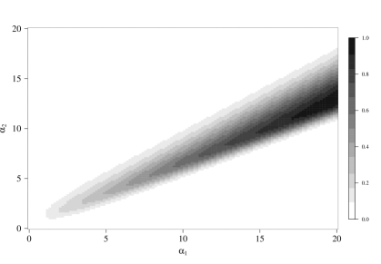
Figure 1: An example of an ill-behaved likelihood function.

Figure 1 depicts the contour plot of the likelihood function for $\text{$\alpha$}=(\alpha_{1},\alpha_{2})$; it is clear that the MLE of the vector $\alpha$ is infinite: the R function msn.mle in the suite sn provides the estimates

$$(\hat{\alpha}_{1},\hat{\alpha}_{2})=(24776144,19911143).$$

The unsatisfactory behaviour of the maximum likelihood method is not immediate clear from the sample values. Table 3 in Eling (2012) shows an even more dramatic example with real data in the context of the skew-$t$ model.

To emphasize this point, we have generated 2000 samples of size 30 from a $SN_{2}$ density with $\text{$\xi$}=(0,0)$, $\Sigma=I_{2}$ and $\text{$\alpha$}=(2,2)$. Point estimates of the shape vector have been obtained, based on the R suite sn, which can be considered as a benchmark in this context. Out of 2000 samples, about $38\%$ resulted in an infinite estimate for $\alpha$; Figure 2 shows the subset of the finite point estimates for $\alpha$. Of course, this admittedly unsatisfactory behaviour tends to be even worse for smaller sample sizes and/or for larger values of $\alpha$. While in the scalar case the set of samples producing infinite ML estimates of $\alpha$ (or $\mid\delta\mid=1$) can be exactly characterized (Liseo and Loperfido, 2006), the detection of such cases in the multivariate case is more complicated.

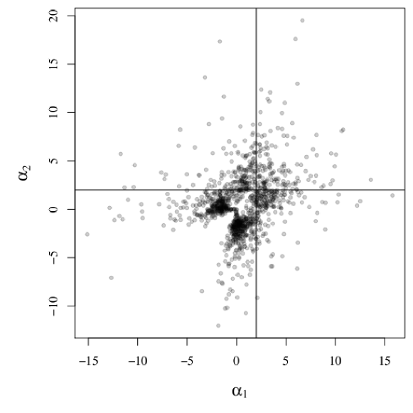
Figure 2: Sampling distribution of the (finite-valued) maximum likelihood estimates of $\alpha$. Solid lines indicate the true value.

A theoretical justification for the unsatisfactory behaviour of the maximum likelihood estimates is that the symmetrized Kullback-Leibler divergence between two $SN_{p}$ densities with similar values of $\alpha$ tends to be very small; this fact typically produces a profile likelihood for $\alpha$ which is rather flat over a large portion of the parameter space. Another way of interpreting the difficulties of a likelihood approach, at least in a simple setting, is the following. For a fixed positive value $z$, consider, as a function of $\alpha$, the likelihood ratio between a standard normal density and an $SN(0,1,\alpha)$ one, with positive $\alpha$, that is

$$LR(\alpha)=\frac{\varphi(z)}{2\varphi(z)\text{$\Phi$}(\alpha z)}=\frac{1}{2\text{$\Phi$}(\alpha z)}.$$

Since $LR(\alpha)$ is decreasing, for any fixed positive $z$, in $(0,\infty)$, its possible values range from $0.5$ (when $\alpha\rightarrow\infty$, that is for a half-normal density) to 1 (for $\alpha=0$); in other words the ability of the likelihood to discriminate between a normal and a skew-normal model seems quite limited. One possibility is then to switch to the production of valid interval estimates. However, solid classical and likelihood theories of confidence intervals for the $SN_{p}$ model are still lacking. Another technical inferential problem with the SN model is that the likelihood function may be multimodal when both the location and the shape parameters are unknown: we will discuss this issue below in this section.

For all these reasons, we propose a full Bayesian analysis of the multivariate SN model. A Bayesian analysis based on objective priors has already been proposed by Liseo and Loperfido (2006) for the scalar case. See also Wiper et al. (2008) for an objective Bayesian analysis in the half-normal and half-$t$ cases, and Branco et al. (2013a) for the skew-$t$ case. Frühwirth-Schnatter and Pyne (2010) have recently proposed a fully Bayesian analysis of a mixture of skew-normal and skew-$t$ densities. Other recent and important advances in the application of multivariate skew-normal models can be found in Fung and Seneta (2010), Panagiotelis and Smith (2010), Ferraz and Moura (2012) and Cabral et al. (2012).
The computational approach described in Frühwirth-Schnatter and Pyne (2010) differs from ours in two respects: i) they adopt conjugate priors in order to facilitate a Gibbs sampling strategy for simulating from the posterior; ii) as a consequence of i), we adopt a different sampling strategy, based on importance sampling rather than MCMC; we will describe the PMC algorithm in detail in Section 4. For the moment we explain why we are not completely confident with the use of Gibbs-type algorithms for skew-normal or skew-$t$ models. It is a well-known fact that likelihood functions arising from a skew-normal model may be multimodal. In these situations, the Gibbs sampler chains are often captured by one of the modes. As a consequence, the chains do not mix well and the posterior distribution is not well explored.

As a practical illustration of the problem, Figure 3 presents the 1000 draws obtained from a Gibbs sampler - similar to that proposed in Frühwirth-Schnatter and Pyne (2010) - in the very simple setting of a scalar skew-normal model with unknown location $\xi$ and shape $\alpha$, and a known scale parameter $\omega=1$. Almost all posterior draws belong to the same mode and the posterior distribution is not well explored.

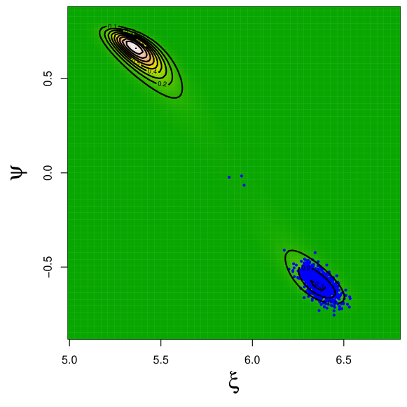
Figure 3: Scalar skew-normal example; posterior distribution for $(\xi,\psi)$ - where $\psi=\omega\alpha/\sqrt{1+\alpha^{2}}$ and 1000 values drawn from a Gibbs algorithm.

In the multidimensional case, things tend to be more complicated; as we will argue in Section 3.1, constraints in the parameter space should be introduced in order to obtain a positive definite correlation matrix, and accounting for them in the Gibbs sampling algorithm may not be easy.

3 Augmented likelihood function and priors

3.1 Introducing the latent structure

In this section we describe how to exploit the intrinsically latent structure of the SN density function in order to produce an augmented likelihood function. The main proposition follows.

Proposition 1

Let $\Omega$ be a correlation matrix, $\delta$ a $p$-dimensional vector and ${\text{$\alpha$}}=(1-\text{$\delta$}^{T}\text{$\Omega$}^{-1}\text{$\delta$})^{-\frac{1}{2}}\text{$\Omega$}^{-1}\text{$\delta$}$. Define

$$\binom{Z}{\mathbf{X}}\sim N_{p+1}\left[\binom{0}{\text{$0$}},\left(\begin{array}[]{c c}1&\text{$\delta$}^{T}\\ \text{$\delta$}&\text{$\Omega$}\end{array}\right)\right]\mbox{ and }\mathbf{U}=\begin{cases}\mathbf{X}&Z\geq 0\\ -\mathbf{X}&Z<0\end{cases}.$$

Then, (a) the random vector ${\mathbf{Y}=\text{$\omega$}\mathbf{U}+\text{$\xi$}}\sim SN_{p}(\text{$\Sigma$},\text{$\xi$},\text{$\alpha$})$, with $\text{$\Sigma$}=\text{$\omega$}\text{$\Omega$}\text{$\omega$},$ and (b) the joint density of $(\mathbf{Y},Z)$ is given by

$$f_{p+1}\left(\mathbf{y},z\right)=f_{p}(\mathbf{y}\mid z)f(z)={N_{p}\left(\text{$\xi$}+\text{$\omega$}\text{$\delta$}\mid z\mid,\text{$\omega$}(\text{$\Omega$}-\text{$\delta$}\text{$\delta$}^{\prime})\text{$\omega$}\right)}\,\times N_{1}(0,1).$$

Proof: (a): From one of the possible definitions of a multivariate $SN$ r.v., it is known that $\mathbf{U}\sim SN_{p}(\text{$\Omega$},\text{$0$},\text{$\alpha$})$; $\mathbf{Y}$ is a simple linear transformation of $\mathbf{U}$ and its distribution is readily obtained.
(b): Start from $f(y,z)=f(z)f(y\mid z)$. Then $f(z)$ is, by assumption, a standard Gaussian density, while

$$\left(\mathbf{Y}\mid Z=z\right)=\left(\text{$\omega$}\mathbf{U}+\text{$\xi$}\mid Z=z\right)=\begin{cases}\text{$\omega$}\mathbf{X}+\text{$\xi$}&z\geq 0\\ -\text{$\omega$}\mathbf{X}+\text{$\xi$}&z<0\\ \end{cases}.$$

Then, by using simple results on conditional Gaussian densities, one gets

$$\left(\mathbf{Y}\mid Z=z\right)\sim\begin{cases}N_{p}\left(\text{$\xi$}+\text{$\omega$}\text{$\delta$}z,\text{$\omega$}(\text{$\Omega$}-\text{$\delta$}\text{$\delta$}^{\prime})\text{$\omega$}\right)&z\geq 0\\ N_{p}\left(\text{$\xi$}-\text{$\omega$}\text{$\delta$}z,\text{$\omega$}(\text{$\Omega$}-\text{$\delta$}\text{$\delta$}^{\prime})\text{$\omega$}\right)&z<0\\ \end{cases}.$$

Using the above proposition one can write an augmented likelihood function, “as if” we had observed, for each sample unit, the latent value $z_{i}$, $i=1,\dots,n$. Write $\text{$\psi$}=\text{$\omega$}\text{$\delta$}$ and $\text{$\omega$}(\text{$\Omega$}-\text{$\delta$}\text{$\delta$}^{\prime})\text{$\omega$}={\text{$\Sigma$}-\text{$\psi$}\text{$\psi$}^{\prime}}=\mathbf{G};$ define the parameter vector as $\text{$\theta$}^{\ast}=(\text{$\delta$},\text{$\Sigma$},\text{$\xi$})$ or $\text{$\theta$}=(\text{$\psi$},\mathbf{G},\text{$\xi$})$. The augmented likelihood function is then

$${L(\text{$\theta$};\mathbf{y},\mathbf{z})} \propto \prod_{i=1}^{n}\left\{\varphi_{p}(\mathbf{y}_{i}-\text{$\xi$}-\text{$\psi$}\,\mid z_{i}\mid;\text{$\Sigma$}-\text{$\psi$}\text{$\psi$}^{\prime})\times\varphi_{1}(z_{i};1)\right\}$$

$$= {\frac{1}{\mid\mathbf{G}\mid^{\frac{n}{2}}}\exp\left(-\frac{1}{2}\sum_{i=1}^{n}z_{i}^{2}\right)}$$

$$\times \exp\left(-\frac{1}{2}\sum_{i=1}^{n}(\mathbf{y}_{i}-\text{$\xi$}-\text{$\psi$}\mid z_{i}\mid)^{\prime}\mathbf{G}^{-1}(\mathbf{y}_{i}-\text{$\xi$}-\text{$\psi$}\mid z_{i}\mid)\right).$$

Notice that the matrix $\mathbf{G}$ must be positive definite; this implies a logical constraint among the values of $\delta$ and $\Omega$ in the original parameterization which should be taken into account when exploring the parameter space via simulation methods. As we have already noticed, this issue seems to have been neglected in literature. See Azzalini’s website http://azzalini.stat.unipd.it/SN/, under the section “A less frequent question” for a graphical treatment of this problem. In particular, MCMC methods should be used with care in order to avoid the chain in the $(\text{$\delta$},\text{$\Omega$})$ parameterization visiting inadmissible parts of the parameter space.

3.2 Prior distributions

Our primary goal here is to propose a general method of inference for the parameters of the multivariate SN distribution. For these reasons we have tried to be as “objective” as possible in choosing the prior for the parameter vector. However, it is not easy to derive a formal Jeffreys or reference prior for the parameters of a multivariate skew-normal distribution. In this paper we have assumed a priori, as usual, $\text{$\xi$}\mathchoice{\mathrel{\hbox to0.0pt{$\displaystyle\perp$\hss}\mkern 2.0mu{\displaystyle\perp}}}{\mathrel{\hbox to0.0pt{$\textstyle\perp$\hss}\mkern 2.0mu{\textstyle\perp}}}{\mathrel{\hbox to0.0pt{$\scriptstyle\perp$\hss}\mkern 2.0mu{\scriptstyle\perp}}}{\mathrel{\hbox to0.0pt{$\scriptscriptstyle\perp$\hss}\mkern 2.0mu{\scriptscriptstyle\perp}}}(\text{$\delta$},\text{$\Sigma$})$. Also we have assumed a flat prior for the “location” parameter $\xi$ and a conjugate normal Inverse Wishart prior for the “scale” parameter $\Sigma$, that is

$$\pi(\text{$\xi$})\propto 1\qquad\mbox{ and }\qquad{\text{$\Sigma$}\sim IW_{p}(m,\text{$\Lambda$})}.$$

Obviously, one can always consider the limiting case ($m\rightarrow 0,\text{$\Lambda$}\rightarrow\text{$0$}$) to get the classical Jeffreys prior

$$\pi(\text{$\xi$},\text{$\Sigma$})\propto\frac{1}{\mid\text{$\Sigma$}\mid^{\frac{p+1}{2}}}.$$ (4)

The choice of a good objective prior for $\delta$ (or $\alpha$) is more delicate. Liseo and Loperfido (2006) have shown that, in the univariate SN model, the Jeffreys’ prior for the shape parameter $\alpha$ is proper; its use, in a sense, automatically and pragmatically solves the problem of a potentially non vanishing likelihood function, which can happen with the skew-normal model (Azzalini and Capitanio, 1999). Branco and Bayes Rodriguez (2007) have shown that the Jeffreys’ prior can be adequately approximated by a Student $t$ density with a half degree of freedom, centered at zero and with scale parameter $\pi^{2}/4$. Branco et al. (2013b), in an as yet unpublished technical report, have partially generalised the above results to the bivariate case, but no general results are available for the $SN_{p}$ model with $p>2$. They have proved that, unlike the scalar case, the Jeffreys’ prior is improper in the bivariate case. On the other hand the one-at-a-time reference prior (Berger and Bernardo, 1992) is proper although its expression is quite complicated. In particular, the Jeffreys’ prior in the $\alpha$ parameterization (using the same approximation provided by Branco and Bayes Rodriguez (2007) for the scalar case) is

$$\pi^{J}(\alpha_{1},\alpha_{2})\propto\frac{1}{1+\pi^{2}/2(\alpha_{1}^{2}+\alpha_{2}^{2})}.$$

The proper reference prior when $\alpha_{1}$ is the parameter of interest and $\alpha_{2}$ is considered a nuisance parameter is given by $\pi^{R}(\alpha_{2}\mid\alpha_{1})\pi^{R}(\alpha_{1})$ where

$$\pi^{R}(\alpha_{2}\mid\alpha_{1})\propto\frac{\left(1+2\eta^{2}\alpha_{1}^{2}\right)^{1/4}}{\left(1+2\eta^{2}(\alpha_{1}^{2}+\alpha_{2}^{2})\right)^{3/4}}\frac{1}{\sqrt{\left(1+2\eta^{2}\alpha_{1}^{2}\right)}}$$ (5)

and

$$\pi^{R}(\alpha_{1})\propto\exp\left(-\frac{1}{4}\int\log\left(1+2\eta^{2}(\alpha_{1}^{2}+t^{2})\right)\pi_{R}(t\mid\alpha_{1})dt\right),$$ (6)

where $\eta=\pi/2$. Of course, when $\alpha_{2}$ is the parameter of interest the prior is the same with $\alpha_{1}$ and $\alpha_{2}$ switching their roles. The above considerations show that an objective analysis can be made only for one component of the shape vector: to get a proper posterior with sampling probability $1$, in the multivariate case, one should introduce genuine prior information for some of the components of $\alpha$. For practical purposes, a prior can be chosen in the following way: in the scalar case the approximate Jeffreys’ prior for $\beta=(1+\delta)/2$, with $\delta=\alpha/\sqrt{1+\alpha^{2}}$, is a Beta$(0.25,0.25)$ prior; in analogy with that, one can use, in the multivariate case, the prior

$$\pi^{IND}(\text{$\delta$})\propto\prod_{j=1}^{p}\left(1-\delta_{j}^{2}\right)^{-\frac{3}{4}},$$ (7)

that is, we assume that the components of the skewness vector are, a priori, independent and identically distributed. Although independence can be considered a strong assumption, it is hard to conceive any non subjective form of dependence. Alternatively, the use of a uniform prior in the $\delta$ parameterization, especially for $p>2$, could be suggested. Using the Jacobian

$$\left|\frac{\partial\text{$\delta$}}{\partial\text{$\alpha$}}\right|=\frac{\mid\text{$\Omega$}\mid}{\left(1+\text{$\alpha$}^{\prime}\text{$\Omega$}\text{$\alpha$}\right)^{2}},$$

the uniform prior in the $\delta$ parameterization is transformed into

$$\pi^{U}(\text{$\alpha$})\propto\frac{1}{(1+\text{$\alpha$}^{\prime}\text{$\Omega$}\text{$\alpha$})^{2}},$$ (8)

which explicitly introduces a dependence on the correlation matrix $\Omega$. Notice also that any prior distribution on $\delta$ should be considered only for those values which satisfy the constraints illustrated at the end of section 3.1. In this perspective, for computational reasons, we will consider the parameter constraint as generated from the prior rather than from the likelihood. In the rest of the paper, we will then consider, as the prior for $\delta$,

$$\tilde{\pi}^{IND}(\text{$\delta$}\mid\text{$\Omega$})=\frac{1}{A(\text{$\Omega$})}\prod_{j=1}^{p}\left(1-\delta_{j}^{2}\right)^{-\frac{3}{4}},$$ (9)

where $A(\text{$\Omega$})$ is the integral of (7) over the parameter values such that $\det(\mathbf{G})>0$. In fact, it is important to notice that, given the hierarchical structure of the prior for $\delta$, one needs to recover the normalizing constant $A(\text{$\Omega$})$. This is analitically feasible only for particular choices of $\pi(\text{$\delta$}\mid\text{$\Omega$})$. In all other cases, one needs to evaluate the integral of $\pi(\text{$\delta$}\mid\text{$\Omega$})$ on the ellipsoid determined by the constraint.

We now give some details about the evaluation of $A(\text{$\Omega$})$ when $p=2$. Generalizations to higher dimensions are similar, although more complicated. In a bivariate setup, we define $\rho$ to be the off-diagonal element of $\Omega$; the constraint produces an ellipse which is a proper subset of the square $[-1,1]^{2}$ (see figure 4, left panel): the shape of the ellipse is a function of $\rho$.

Figure 4: Left panel: different shapes of the parameter space of $\delta$ for different values of $\rho$. Right panel: dots represent numerical evaluations of $A(\text{$\Omega$})$ for different values of $\rho$, the solid curve represents the approximation given in eq. (10). Vertical lines denote the same values of $\rho$ considered in the left panel.

$A(\text{$\Omega$})$ can be evaluated on a grid of values of $\rho$, for example using a rejection sampler where the simulated values of $\delta$ are generated by two independent $\textrm{Beta}({0.1,0.1})$ deviates. The choice of the proposal is due to the fact that the Jeffreys’ prior puts most of the probability mass on the boundary of the square. Results on a grid of values of $\rho$ are represented in the right panel of fig. 4 by dots. This approach can be computationally demanding. For practical purposes, a very satisfactory approximation can be obtained using the formula

$$A(\text{$\Omega$})\approx a\,(1-\rho^{2})^{b}.$$ (10)

Estimation of $a$ and $b$ is then straightforward. We have obtained $a$ = 6.68 and $b$ = 0.28.

Although the above defined $\text{$\theta$}^{\ast}$ parameterization is more suitable for elicitation, the alternative $\theta$ parameterization should be preferred in terms of implementation and computation. From now on, we will use $\text{$\theta$}=(\text{$\psi$},\mathbf{G},\text{$\xi$})$. This can be simply done by introducing a Jacobian term in the prior, namely

$$J(\text{$\theta$}^{\ast}\to\text{$\theta$})=\prod_{j=1}^{p}\left(G_{jj}+\psi_{j}^{2}\right)^{-\frac{1}{2}}.$$ (11)

4 Population Monte Carlo algorithm

In this section we illustrate a PMC algorithm for obtaining a sample from the joint posterior distribution of $\theta$. PMC methods (see e.g. Cappé et al., 2004) essentially consist of an iterated version of the importance sampling algorithm: at each iteration, a population of particles is generated, independently of each other, possibly using a set of different importance functions. Performances obtained in the past iterations by the different kernels are typically evaluated in a relative way in order to adaptively modify the proposal distributions over the iterations.
Alternatively, Celeux et al. (2006) suggest the use of the full conditional distributions as the importance functions when the model at hand has a latent structure representation, as in the present case. This way, one can exploit the easiness of proposing from a natural importance function, i.e. the full conditional, and, at the same time, avoid the convergence issues of a generic MCMC method. Also, the coexistence of different particles, and the competition between them, allows us to tackle better the issue of multimodality of the posterior density. It is well known that in similar situations the Gibbs sampler tends to be attracted by one of the modes and hardly escapes from a neighborhood of it (Celeux et al., 2000).

From a model selection perspective, the estimation of the normalising constant of $\pi(\text{$\theta$}|\mathbf{y})$ can be performed as a simple by-product of any PMC (and MC) sampler. In fact, from the importance sampling identity, one obtains

$$p(\mathbf{y})=\int_{\text{$\Theta$}}\int_{\mathcal{Z}}\pi(\text{$\theta$},\mathbf{z},\mathbf{y})d\text{$\theta$}d\mathbf{z}=\int_{\text{$\Theta$}}\int_{\mathcal{Z}}\frac{\pi(\text{$\theta$},\mathbf{z},\mathbf{y})}{q(\text{$\theta$},\mathbf{z})}q(\text{$\theta$},\mathbf{z})d\text{$\theta$}d\mathbf{z},$$

where $q$ is the proposal distribution. Adopting the usual Monte Carlo approximation, $p(\mathbf{y})$ can be estimated by

$$\hat{p}(\mathbf{y})\approx\frac{\sum_{t=1}^{T}H_{t}\sum_{i=1}^{N}\tilde{\zeta}_{i}^{(t)}}{N\sum_{t=1}^{T}H_{t}},$$ (12)

where the $\tilde{\zeta}_{i}$’s denote the unnormalised importance weights, and

$$H_{t}=-\sum_{i=1}^{N}\zeta_{i}^{(t)}\log(\zeta_{i}^{(t)}).$$ (13)

is an entropy measure of performance of the $t$-th iteration of the algorithm. $H_{t}$ takes high values when the normalised weights of the particles in the $t$-th iteration are concentrated around $1/N$. The quantity (13) is a monotonic transformation of the perplexity measure (Robert and Casella, 2010), defined as $\exp(H_{t})/N$. We will use the perplexity index as a measure of non degeneracy of the PMC algorithm, which is often considered as one potential drawback of Monte Carlo methods. Last but not least, the use of PMC algorithms allows the simultaenous draw of all the particles: this fact dramatically improves the efficiency of the algorithm compared with generic MCMC approaches. The estimator (12) is quite simple and stable since it does not rely upon convergence issues. A possible improvement on (12) can be obtained via the Adaptive Multiple Importance sampling technique, Cornuet et al. (2012). The difference with PMC is that, in this case, the importance weights of all simulated values, past as well as present, are recomputed at each iteration. We are currently working on these aspects.

Without loss of generality, we illustrate the steps of the algorithm for a bidimensional setup. The generalization to higher dimensional problems is straightforward, even though numerical problems can arise with some choices of the prior for $\delta$, and care must be taken in handling the approximation of $A(\text{$\Omega$})$. In the simulation study described in Section 7 we reported perplexities of our samples, although we have never experienced significant problems in terms of degeneracy: however we recognize that this can be a critical issue when the proposal densities are not well calibrated.

After approximating $A(\text{$\Omega$})$, the PMC algorithm can be initialised by sampling random starting particles. These particles will be updated in the following iterations using, as proposal distributions, the full conditionals (when available in closed form) or some other distributions which approximate them.
In particular, the full conditional distributions of the latent variables $Z_{i}$’s (see figure 5) are symmetric about the origin:

$$f(z_{i}|\cdots)=\left\{\begin{array}[]{lll}\varphi(z_{i}-m_{i};v)&\rule{5.69046pt}{0.0pt}&z_{i}\geq 0\\ \varphi(z_{i}+m_{i};v)&\rule{5.69046pt}{0.0pt}&z_{i}<0\\ \end{array}\right.,$$

Figure 5: Some examples of the full conditional distribution of a generic $z_{i}$ for different values of $m_{i}$.

where

$$v=(1+\text{$\psi$}^{\prime}\mathbf{G}^{-1}\text{$\psi$})^{-1},$$

and $m_{i}$ is the $i$-th component of the vector

$$\mathbf{m}=v\left[(\mathbf{y}-\mathds{1}_{n}\otimes\text{$\xi$})^{\prime}\mathbf{G}^{-1}\text{$\psi$}\right].$$

It is not necessary to sample the signs of $Z_{i}$’s, as $\mathbf{z}$ is involved in the posterior distribution only with its absolute value, and the full conditional distribution of $|z_{i}|$ is just a truncated normal. Nevertheless, we prefer to directly sample the value of $\mathbf{z}$, as potential asymmetries in the posterior draws could highlight potential problems in the sampler. Hence, we only have to sample the sign (each sign having probability 1/2) independently of $|z_{i}|$. Generation of the $z_{i}$’s can be done using several methods; troubles can arise when $m_{i}/v^{1/2}$ takes large negative values: in this case, sampling from the very extreme tail of a normal distribution using an accept-reject algorithm can be intensive while the inversion method may give numerically unreliable results; in these cases we have employed the approach described in Philippe and Robert (2003), essentially a perfect sampling algorithm.

Simple algebra leads to the full conditional for $\xi$:

$$\left[\text{$\xi$}|\cdots\right]\sim N_{p}(\bar{\mathbf{y}}-\text{$\psi$}\overline{|\mathbf{z}|},\mathbf{G}/n),$$

where $\bar{\mathbf{y}}$ is the sample mean vector, and $\overline{|\mathbf{z}|}$ is the mean of the absolute values of the $z_{i}$’s. Finally, $\mathbf{G}$ and $\psi$ have non-standard full-conditional distributions:

$$\pi(\mathbf{G}|\cdots)\propto\pi(\mathbf{G})IW_{p}(n+m,\text{$\Lambda$}_{\star}),$$

where $\pi(\mathbf{G})$ is the prior for $\mathbf{G}$ arising from (4) and a Jacobian argument, and

$$\text{$\Lambda$}_{\star}=\text{$\Lambda$}+\sum_{i=1}^{n}(\mathbf{y}_{i}-\text{$\psi$}|z_{i}|-\text{$\xi$})(\mathbf{y}_{i}-\text{$\psi$}|z_{i}|-\text{$\xi$})^{\prime}.$$

We use a $IW_{p}(n+m,\text{$\Lambda$}_{\star})$ distribution (which is the one obtained by the full conditional distribution ignoring the contribution of the prior) to propose values for $\mathbf{G}$, as this distribution will resemble the full conditional, in particular for large sample sizes. Finally, the full conditional distribution of $\psi$ is proportional to

$$\pi(\text{$\psi$}|\cdots)\propto\pi(\text{$\psi$}|\text{$\Omega$})\varphi_{p}\left(\text{$\psi$}-\frac{\sum_{i=1}^{n}|z_{i}|(\mathbf{y}_{i}-\text{$\xi$})}{\sum_{i=1}^{n}z_{i}^{2}};\frac{\mathbf{G}}{\sum_{i=1}^{n}z_{i}^{2}}\right).$$

In this case, it is possible to consider several proposal distributions; in order to minimize the computational burden, we propose to sample values from the $p$-variate normal “part” of the full conditional distribution.

As usual, we compute the importance weights $\tilde{\boldsymbol{\zeta}}$ as the ratio $\tilde{\pi}(\text{$\theta$},\mathbf{z}\mid\mathbf{y})/q(\text{$\theta$},\mathbf{z})$, where $\tilde{\pi}$ is the posterior density in which the prior for $(\text{$\psi$}\mid\text{$\Omega$})$ has been (approximately) normalised, and $q$ is the joint proposal density. Particles will be multinomially resampled with unnormalised weights given by $\tilde{\boldsymbol{\zeta}}$ and the resampled particles will represent the starting point for the particles of the next iteration.

5 Bayes factor

One of the main reasons for the popularity of the multivariate skew-normal model is that it represents a proper generalization of the multivariate normal model. Then it is often important to test the normality of the dataset versus skew-normal alternatives. Here we will use the Bayes factor to compare the multivariate Gaussian model - say $M_{0}$ - versus the multivariate skew-normal one - say $M_{1}$. To this end, we need to evaluate the predictive distribution of the data under the two competing models. Suppose that, under model $M_{0}$, $\psi$ is set equal to $\mathrm{𝟎}$. Then the model is described by the following assumptions:

• $Y_{1},\dots,Y_{n}\stackrel{{\scriptstyle\texttt{iid}}}{{\sim}}N_{p}(\text{$\xi$},\text{$\Sigma$})$;

• $\pi^{J}(\text{$\xi$},\text{$\Sigma$})=\mid\text{$\Sigma$}\mid^{-(p+1)/2}$;

it is a standard calculation to show that the marginal distribution of the data under the normal model is

$$p_{0}(\mathbf{y})=\int_{\text{$\Sigma$}}\int_{\text{$\xi$}}\varphi_{p}(\mathbf{y}-\text{$\xi$};\text{$\Sigma$})\pi^{J}(\text{$\xi$},\text{$\Sigma$})d\text{$\Sigma$}d\text{$\xi$}=\frac{2^{n/2}\Psi_{p}((n-1)/2)}{\pi^{p(n-p-1)/4}\mid S\mid^{(n-1)/2}n^{n/2}},$$ (14)

where $S$ is the sample covariance matrix and

$$\Psi_{p}(u)=\prod_{j=1}^{p}\Gamma\left(u-\frac{1}{2}(j-1)\right)$$

is the multivariate Gamma function. Notice that, since the Jeffreys’ prior $\pi^{J}(\text{$\xi$},\text{$\Sigma$})$ is improper, quantity (14) is meaningless per se. However, if we use the same - improper - prior for the common parameters of the two models (in this case $\xi$ and $\Sigma$), then the Bayes factor is a well-defined tool for model comparison.

To compute the Bayes factor $B_{10}$ for comparing the skew-normal model and the nested normal model we need an estimate $\hat{p}_{1}(\mathbf{y})$ of $p_{1}(\mathbf{y})$, the marginal distribution of data under the skew-normal hypothesis. We then perform $T$ iterations of PMC algorithm and we sample $N$ particles in each iteration. Using (12), the final estimate of the Bayes factor is then

$$B_{10}\approx\frac{\sum_{t=1}^{T}H_{t}\sum_{i=1}^{N}\tilde{\zeta}_{j}^{(t)}}{p_{0}(\mathbf{y})N\sum_{t=1}^{T}H_{t}}.$$ (15)

6 Some discussion and extensions

The computational approach we have discussed in the previous sections can be easily adapted to more general situations. In the presence of $k$ covariates, the location parameter vector $\xi$ should be replaced by a $k\times p$ matrix of regression coefficients $\mathbf{B}$, so that our model gets transformed into

$$\mathbf{y}_{i}\stackrel{{\scriptstyle\texttt{iid}}}{{\sim}}SN(\mathbf{G},\mathbf{X}_{i}^{\prime}\mathbf{B},\text{$\psi$}),\qquad i=1,2,\ldots,n.$$

The augmented likelihood for this new model is then

$$L(\mathbf{B},\mathbf{G},\text{$\psi$}|\mathbf{Y},\mathbf{z}) \propto |\mathbf{G}|^{-n/2}\exp\left\{-\frac{1}{2}\mathbf{z}^{\prime}\mathbf{z}\right\}$$

$$\exp\left\{-\frac{1}{2}\sum_{i=1}^{n}(\mathbf{y}_{i}-\mathbf{X}_{i}^{\prime}\mathbf{B}-\text{$\psi$}|z_{i}|)^{\prime}\mathbf{G}^{-1}(\mathbf{y}_{i}-\mathbf{X}_{i}^{\prime}\mathbf{B}-\text{$\psi$}|z_{i}|)\right\}.$$

The previous PMC sampler is still valid for this model; the only necessary modification is the introduction of a proposal step for $\mathbf{B}$ in lieu of $\xi$. Adopting a flat prior for the elements of the matrix $\mathbf{B}$, we again use the full conditional distribution of $\mathbf{B}$ as our proposal. It is easy to show that

$$[\mathbf{B}|\cdots]\sim MN(\mathbf{S}^{-1}\mathbf{C}_{\text{$\psi$}},\mathbf{S}^{-1},\mathbf{G}),$$

where

$$\mathbf{S}=\sum_{i=1}^{n}\mathbf{X}_{i}\mathbf{X}_{i}^{\prime},\qquad\mathbf{C}_{\text{$\psi$}}=\sum_{i=1}^{n}\mathbf{X}_{i}(\mathbf{y}_{i}-|z_{i}|\text{$\psi$})^{\prime},$$

and the symbol $MN(\mathbf{M},\mathbf{R},\text{$\Delta$})$ refers to a matrix normal random variable $\mathbf{V}$ (Dawid, 1981), with location $\mathbf{M}$ and scale parameters $\mathbf{R}$ and $\Delta$, with density:

$$f(\mathbf{V}|\mathbf{M},\mathbf{R},\text{$\Delta$})=\frac{\exp\left\{\frac{1}{2}\operatorname{tr}[\mathbf{R}^{-1}(\mathbf{V}-\mathbf{M})^{\prime}\text{$\Delta$}^{-1}(\mathbf{V}-\mathbf{M})]\right\}}{(2\pi)^{np/2}|\mathbf{R}|^{n/2}|\text{$\Delta$}|^{p/2}}.$$

Simulating draws from this distribution is simple, as it is linked with the multivariate normal distribution by a simple relation:

$$\mathbf{V}\sim MN_{n\times p}(\mathbf{M},\mathbf{R},\text{$\Delta$})\mbox{ if and only if }\operatorname{vec}(\mathbf{V})\sim N_{np}(\operatorname{vec}(\mathbf{M}),\mathbf{R}\otimes\text{$\Delta$}),$$

where $\otimes$ denotes the Kronecker product.

The Bayesian approach through data augmentation is also particularly useful in problems with missing data. Our algorithm can be easily adapted to account for missingness and a comparison of our approach with the one based on the EM algorithm proposed in Lin and Lin (2011) and Lin et al. (2009) is currently under investigation.

7 Simulations and examples

In this section we consider the frequentist properties of our Bayesian procedure; in particular we simulate samples of size $n_{1}=50$ and $n_{2}=200$ for different combinations of parameter values. In all simulations we have used $20,000$ particles for 20 iterations, setting $\text{$\xi$}=(3,3)^{\prime}$ and $\omega_{1}=\omega_{2}=1$.
Table 1 shows a summary of the results: for each parameter combination we provide

• the frequency of times that $B_{10}$ provides evidence in favour of the normal or the skew-normal model (second and fourth column) or that it does not provide strong evidence for any of the two models (third column);

• the median of the simulated sampling distribution of the posterior median (fifth column);

• the frequentist coverage of the one-sided 0.95% and 0.9% credible sets (columns $FC_{0.95}$ and $FC_{0.9}$);

• the median of the sampling distributions of the posterior mean $\operatorname{\rm IE}\left(\psi_{1}|\mathbf{y}\right)$ (eighth column, denoted by MeMean), Conditional (on the true $z_{i}$’s) MLE (ninth column, denoted by MeCMLE) and MLE (tenth column, denoted by MeMLE);

Results for the skewness parameter are shown for the first component of the vector $\text{$\psi$}_{1}$; similar results are obtained for $\text{$\psi$}_{2}$. As might be expected, both the likelihood and Bayesian approaches successfully estimate the off-diagonal element of $\mathbf{G}$, while estimation of $\psi$ - and, consequently, of $\xi$ - seems more difficult. Table 1 highlights the difficulties in catching skewness in small datasets, which implies a high rate of wrong answers given by Bayes factors for non-normal samples. With respect to the ML estimator, it should be noticed that, even though the medians of the sampling distributions of the MLE are quite precise, this estimator always shows a non-negligible probability of producing infinite estimates.

$$\begin{array}[]{cccccccccccc}n=30\\ \lx@intercol\hfil\text{True values}\hfil\lx@intercol&B_{10}<0.5&0.5\leq B_{10}<2&B_{10}\geq 2&Med(Med(\psi_{1}))&FC_{0.95}&FC_{0.9}&MeMean&MeCMLE&MeMLE\\ \hline\cr\text{$\psi$}=0_{2},&\rho=0&(\text{$\alpha$}=0_{2})&0.997&0.003&0.000&0.007&0.983&0.971&0.008&0.010&-0.015\\ \text{$\psi$}=0.5_{2},&\rho=0&(\text{$\alpha$}\approx 0.71_{2})&0.988&0.011&0.001&0.031&0.926&0.874&0.026&0.516&0.085\\ \text{$\psi$}=0.7_{2},&\rho=0&(\text{$\alpha$}\approx 4.95_{2})&0.877&0.098&0.025&0.362&0.806&0.728&0.308&0.696&0.582\\ \text{$\psi$}=0_{2},&\rho=0.5&(\text{$\alpha$}=0_{2})&0.996&0.003&0.001&0.011&0.979&0.959&0.007&0.022&0.123\\ \text{$\psi$}=0.5_{2},&\rho=0.5&(\text{$\alpha$}\approx 0.41_{2})&0.989&0.009&0.002&0.031&0.900&0.852&0.026&0.519&0.146\\ \text{$\psi$}=0.7_{2},&\rho=0.5&(\text{$\alpha$}\approx 0.79_{2})&0.940&0.042&0.018&0.163&0.782&0.660&0.133&0.702&0.385\\ \text{$\psi$}\approx 0.495_{2},&\rho=-0.5&(\text{$\alpha$}=7_{2})&0.958&0.034&0.008&0.161&0.874&0.838&0.116&0.499&0.483\\ &&&&&\\ &&&&&\\ n=200\\ \lx@intercol\hfil\text{True values}\hfil\lx@intercol&B_{10}<0.5&0.5\leq B_{10}<2&B_{10}\geq 2&Med(Med(\psi_{1}))&FC_{0.95}&FC_{0.9}&MeMean&MeCMLE&MeMLE\\ \hline\cr\text{$\psi$}=0_{2},&\rho=0&(\text{$\alpha$}=0_{2})&0.999&0.001&0&-0.002&0.873&0.816&-0.003&-0.007&0.045\\ \text{$\psi$}=0.5_{2},&\rho=0&(\text{$\alpha$}\approx 0.71_{2})&0.995&0.004&0.001&0.211&0.709&0.634&0.187&0.500&0.267\\ \text{$\psi$}=0.7_{2},&\rho=0&(\text{$\alpha$}\approx 4.95_{2})&0.006&0.005&0.989&0.573&0.737&0.635&0.569&0.699&0.687\\ \text{$\psi$}=0_{2},&\rho=0.5&(\text{$\alpha$}=0_{2})&0.999&0.001&0.000&0.027&0.820&0.724&0.031&-0.005&0.071\\ \text{$\psi$}=0.5_{2},&\rho=0.5&(\text{$\alpha$}\approx 0.41_{2})&0.997&0.002&0.001&0.152&0.695&0.601&0.139&0.499&0.183\\ \text{$\psi$}=0.7_{2},&\rho=0.5&(\text{$\alpha$}\approx 0.79_{2})&0.899&0.065&0.036&0.479&0.701&0.624&0.460&0.699&0.664\\ \text{$\psi$}\approx 0.495_{2},&\rho=-0.5&(\text{$\alpha$}=7_{2})&0.008&0.019&0.973&0.385&0.885&0.804&0.382&0.496&0.495\\ \end{array}$$

Table 1: Summary of the results obtained in the simulation study; the rows relative to combinations of parameters that generate high skewness are highlighted in gray.

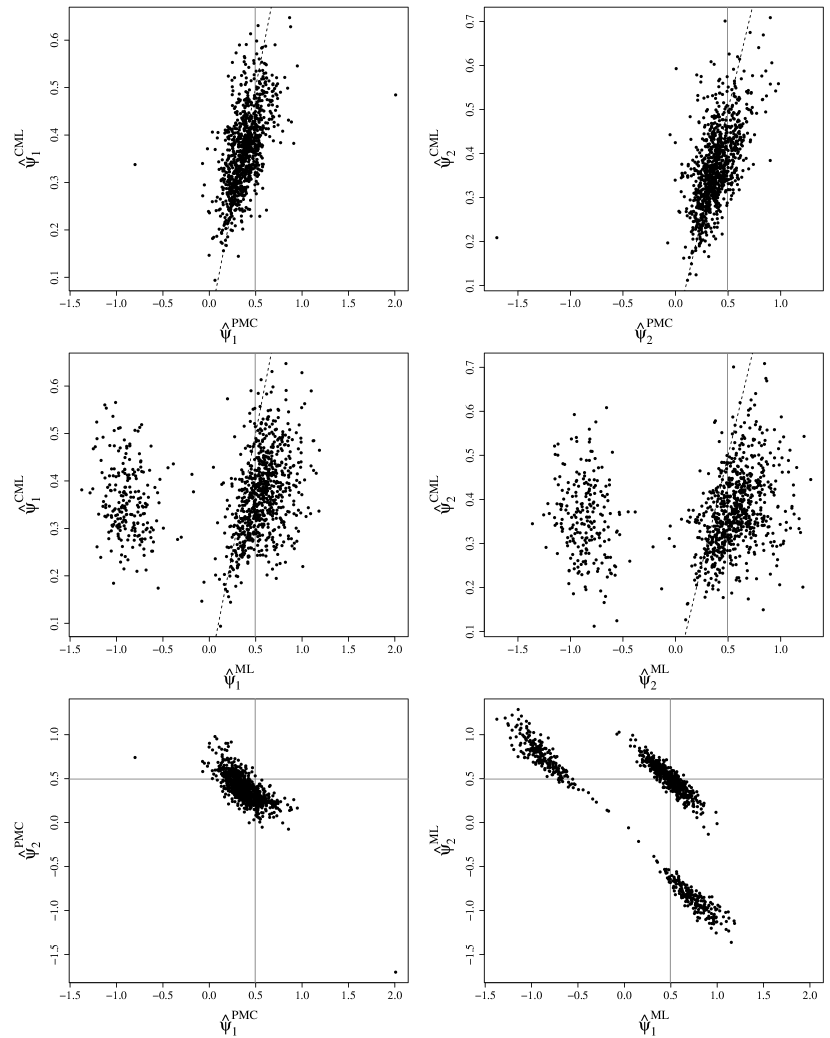
Figure 6: ML, CML, Bayesian estimates and true values of the parameters.

Figure 6 compares the estimates obtained using our approach and the maximum likelihood method in the most extreme combination of parameters, with $\rho=-0.5$, $\text{$\omega$}=(1,1)^{\prime}$ and $\text{$\psi$}=(0.495,0.495)^{\prime}$. The value of $\psi$ lies on the border of the acceptable region and corresponds to $\text{$\alpha$}=(7,7)^{\prime}$. The first row shows a comparison between our Bayesian estimates $\text{$\psi$}_{1}^{PMC}$, and $\text{$\psi$}_{1}^{CML}$, the complete maximum likelihood estimates. These estimates are obtained using the true values of the latent variables $z_{i}$, thus bringing the problem back to a multivariate normal regression model of $\mathbf{y}$ over $|\mathbf{z}|$, in which $\xi$ and $\psi$ play the roles of an intercept and a slope. In fact, for known values of $\mathbf{z}|$, the complete likelihood function reduces to

$$L(\text{$\theta$};\mathbf{y},\mathbf{z})\propto|\mathbf{G}|^{-n/2}\exp\left\{-\frac{1}{2}\sum_{i=1}^{n}(\mathbf{y}_{i}-\text{$\xi$}-\text{$\psi$}|z_{i}|)^{\prime}\mathbf{G}^{-1}(\mathbf{y}_{i}-\text{$\xi$}-\text{$\psi$}|z_{i}|)\right\},$$

and the conditional (on $z$’s) maximum likelihood (CML) estimates are:

$$\hat{\text{$\psi$}}^{CML} = \frac{\sum_{i}(|z_{i}|(\mathbf{y}_{i}-\hat{\text{$\xi$}}^{CML}))}{\sum_{i}z_{i}^{2}};$$

$$\rule{0.0pt}{14.22636pt}\hat{\text{$\xi$}}^{CML} = \bar{\bf y}-\hat{\text{$\psi$}}^{CML}\overline{|\mathbf{z}|};$$

$$\rule{0.0pt}{19.91684pt}\hat{\mathbf{G}}^{CML} = n^{-1}(\overline{\mathbf{y}}-\hat{\text{$\xi$}}^{CML}-\hat{\text{$\psi$}}^{CML}\overline{|\mathbf{z}|})(\overline{\mathbf{y}}-\hat{\text{$\xi$}}^{CML}-\hat{\text{$\psi$}}^{CML}\overline{|\mathbf{z}|})^{\prime}.$$

The CML estimator is to be considered as a benchmark, as it uses an additional piece of information which is not available for ML and PMC estimators.
The PMC estimates are concentrated in a single cloud around the true value and they are in close agreement with the CML estimates. Very few points fall far from the cloud: it is probably a consequence of the multimodality of the posterior distribution.

The second row shows the comparison between ML estimates $\hat{\text{$\psi$}}_{1}^{ML}$ and $\hat{\text{$\psi$}}_{1}^{CML}$. The dashed line is the bisector of the first and third quadrant, and the solid line represents the true value of the parameter. Scatterplots of the ML estimates reveal the odd behaviour of the likelihood, with points in the “genuine” part of the distribution showing a higher variability.
The last row of Figure 6 show the bivariate scatterplots of the Bayesian point estimates $\hat{\text{$\psi$}}^{PMC}$ and of the maximum likelihood estimates $\hat{\text{$\psi$}}^{ML}$, with lines indicating the true values of the parameters. The sampling distribution of $\hat{\text{$\psi$}}^{ML}$ is clearly multimodal. It also shows a larger dispersion and a negative skewness for both $\hat{\psi}_{1}^{ML}$ and $\hat{\psi}_{2}^{ML}$.

Figure 7: Perplexity measures in the first three iterations of the PMC algorithm for a simulation. It shows a typical pattern, with a decreasing number of outlier particles.

7.1 A real dataset

As a final illustration of the proposed algorithm, we analyse the returns of two stocks in the NYSE composite index, namely the “ABM Industries Incorporated” and “The Boeing Company” for the two decades October 1, 1992 to October 1, 2012 (240 monthly observations). Data are available at
http://finance.yahoo.com/q/cp?s=%5ENYA+Components. Data show a moderate degree of skewness.

We have performed a PMC sampler with $25$ iterations, $30,000$ particles each. Figure 8 displays the raw data and the estimated $SN_{2}$ density obtained from our proposed algorithm (left) and from the ML approach (right). Table 2 summarizes the marginal posterior distributions of the parameters.

	$\xi_{1}$	$\xi_{2}$	$\rho$	$\omega_{1}$	$\omega_{2}$	$\psi_{1}$	$\psi_{2}$
1%	0.040	0.042	0.310	0.085	0.086	-0.075	-0.076
5%	0.045	0.049	0.369	0.088	0.090	-0.072	-0.076
50%	0.059	0.061	0.462	0.096	0.095	-0.064	-0.065
95%	0.068	0.068	0.526	0.101	0.102	-0.046	-0.054
99%	0.071	0.072	0.559	0.104	0.104	-0.042	-0.048

Table 2: Marginal posterior quantiles for the parameters of the model.

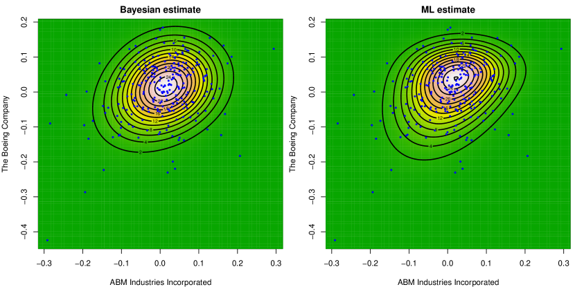
Figure 8: Returns of the stocks and contour plot of the density of the estimated $SN_{2}$ model, using the PMC algorithm (left) and the ML approach (right).

Figure 9 depicts a typical pattern of an MC estimate of the Bayes factor throughout the iterations: at the sixth iteration, a huge jump occurs, probably due to the discovery of a region of high posterior density. This causes a degeneracy of the particles, the production of non reliable estimates and a rise in the perplexity index for that iteration. Once that the new region has been explored, the estimates become stable. The high value of the estimated Bayes factor in the sixth iteration will not affect the final estimate, as it will be downweighted through the perplexity index. Using formula (15), the final estimate of the Bayes factor is $\hat{B}_{10}=500.76$, showing overwhelming evidence in favour of the skew-normal model compared to the normal one.

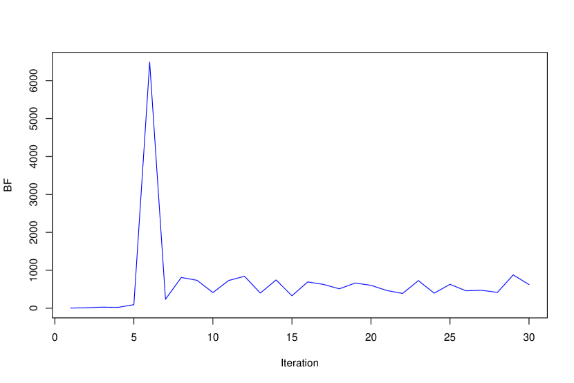
Figure 9: Pattern of the estimated Bayes factor over iterations.

8 Acknowledgements

The Authors are sincerely grateful to an Associate Editor and two anonymous referees whose constructive criticism greatly improved a first version of the present paper. Work supported by the project PRIN 2008: New developments in Bayesian sampling: theory and practice, Project number 2008CEFF37, Sector: Economics and Statistics.

References

- Arellano-Valle and Azzalini (2008) Arellano-Valle, R. B., Azzalini, A., 2008. The centred parametrization for the multivariate skew-normal distribution. J. Multivariate Anal. 99 (7), 1362–1382.
- Arnold and Beaver (2002) Arnold, B. C., Beaver, R. J., 2002. Skewed multivariate models related to hidden truncation and/or selective reporting. Test 11 (1), 7–54, with discussion and a rejoinder by the authors.
- Azzalini (1985) Azzalini, A., 1985. A class of distributions which includes the normal ones. Scand. J. Statist. 12, 171–178.
- Azzalini (2005) Azzalini, A., 2005. The skew-normal distribution and related multivariate families (with discussion). Scand. J. Statistics 32, 159–200.
- Azzalini and Capitanio (1999) Azzalini, A., Capitanio, A., 1999. Statistical applications of the multivariate skew-normal distributions. J. R. Statist. Soc. B 61, 579–602.
- Azzalini and Capitanio (2003) Azzalini, A., Capitanio, A., 2003. Distributions generated by perturbation of symmetry with emphasis on a multivariate skew t distribution. J. R. Statist. Soc. B 65, 367–389.
- Azzalini and Dalla Valle (1996) Azzalini, A., Dalla Valle, A., 1996. The multivariate skew-normal distribution. Biometrika 83, 715–726.
- Berger and Bernardo (1992) Berger, J., Bernardo, J., 1992. On the development of reference priors. Bayesian statistics, 4;(J.O. Berger, J.M. Bernardo, A.P. Dawid and A.F.M. Smith, eds.) Oxford Univ. Press, London, 35–60.
- Branco and Bayes Rodriguez (2007) Branco, M., Bayes Rodriguez, C., 2007. Bayesian inference for the skewness parameter of the skew-normal distribution. Brazilian Journal of Probability and Statistics 21, 141–163.
- Branco et al. (2013a) Branco, M., Genton, M., Liseo, B., 2013a. Objective Bayesian Analysis of Skew-t Distributions. Scandinavian Journal of Statistics (in press).
- Branco et al. (2013b) Branco, M., Genton, M., Liseo, B., 2013b. Objective Bayesian Analysis of the bivariate skew-normal distributions. Manuscript under preparation.
- Cabral et al. (2012) Cabral, C. R. B., Lachos, V. H., Prates, M. O., 2012. Multivariate mixture modeling using skew-normal independent distributions. Comput. Statist. Data Anal. 56 (1), 126–142.
- Cappé et al. (2004) Cappé, O., Guillin, A., Marin, J. M., Robert, C. P., 2004. Population Monte Carlo. J. Comput. Graph. Statist. 13 (4), 907–929.
- Celeux et al. (2000) Celeux, G., Hurn, M., Robert, C., 2000. Computational and inferential difficulties with mixture posterior distributions. Journal of the American Statistical Association 95, 957–970.
- Celeux et al. (2006) Celeux, G., Marin, J.-M., Robert, C. P., 2006. Iterated importance sampling in missing data problems. Comput. Statist. Data Anal. 50 (12), 3386–3404.
- Cornuet et al. (2012) Cornuet, J., Marin, J., Mira, A., Robert, C., 2012. Adaptive Multiple Importance Sampling. Scandinavian Journal of Statistics (to appear)Available as arXiv:0907.1254.
- Dawid (1981) Dawid, A. P., 1981. Some matrix-variate distribution theory: Notational considerations and a Bayesian application. Biometrika 68 (1), 265–274.
- Eling (2012) Eling, M., 2012. Fitting insurance claims to skewed distributions: are the skew-normal and skew-student good models? Insurance Math. Econom. 51 (2), 239–248.
- Ferraz and Moura (2012) Ferraz, V. R. S., Moura, F. A. S., 2012. Small area estimation using skew normal models. Comput. Statist. Data Anal. 56 (10), 2864–2874.
- Frühwirth-Schnatter and Pyne (2010) Frühwirth-Schnatter, S., Pyne, S., 2010. Bayesian inference for finite mixtures of univariate and multivariate skew-normal and skew-t distributions. Biostatistics 11 (2), 317–336.
- Fung and Seneta (2010) Fung, T., Seneta, E., 2010. Modelling and Estimation for Bivariate Financial Returns. International statistical review 78 (1), 117–133.
- Genton (2004) Genton, M. E., 2004. Skew-Elliptical Distributions and Their Applications: A Journey Beyond Normality. CRC/Chapman & Hall, London.
- Lin et al. (2009) Lin, T. I., Ho, H. J., Chen, C. L., 2009. Analysis of multivariate skew normal models with incomplete data. J. Multivariate Anal. 100 (10), 2337–2351.
- Lin and Lin (2011) Lin, T.-I., Lin, T.-C., 2011. Robust statistical modelling using the multivariate skew distribution with complete and incomplete data. Stat. Model. 11 (3), 253–277.
- Liseo (1990) Liseo, B., 1990. La classe delle densità normali sghembe: aspetti inferenziali da un punto di vista bayesiano. Statistica 50, 59–70.
- Liseo and Loperfido (2006) Liseo, B., Loperfido, N., 2006. A note on the reference prior for the scalar skew normal distribution. J. Statist. Plann. Inference 136 (2), 373–389.
- O’Hagan and Leonard (1976) O’Hagan, A., Leonard, T., 1976. Bayes estimation subject to uncertainty about parameter constraints. Biometrika 63, 201–202.
- Panagiotelis and Smith (2010) Panagiotelis, A., Smith, M., 2010. Bayesian skew selection for multivariate models. Computational Statistics and Data Analysis 54, 1824–1839.
- Philippe and Robert (2003) Philippe, A., Robert, C., 2003. Perfect simulation of positive Gaussian distributions. Stat. Comput. 13 (2), 179–186.
- Robert and Casella (2010) Robert, C., Casella, G., 2010. Introducing Monte Carlo Methods with R. Springer.
- Roberts (1966) Roberts, C., 1966. A correlation model useful in the study of twins. Journal of the American Statistical Association 61, 1184–1190.
- Wiper et al. (2008) Wiper, M. P., Girón, F. J., Pewsey, A., 2008. Objective Bayesian inference for the half-normal and half- distributions. Comm. Statist. Theory Methods 37 (18-20), 3165–3185.