Work distribution in time-dependent logarithmic-harmonic potential: exact results and asymptotic analysis

Abstract

We investigate the distribution of work performed on a Brownian particle in a time-dependent asymmetric potential well. The potential has a harmonic component with time-dependent force constant and a time-independent logarithmic barrier at the origin. For arbitrary driving protocol, the problem of solving the Fokker-Planck equation for the joint probability density of work and particle position is reduced to the solution of the Riccati differential equation. For a particular choice of the driving protocol, an exact solution of the Riccati equation is presented. Asymptotic analysis of the resulting expression yields the tail behavior of the work distribution for small and large work values. In the limit of vanishing logarithmic barrier, the work distribution for the breathing parabola model is obtained.

1 Introduction

Stochastic thermodynamics is an advancing field with many applications to small systems of current interest [1, 2, 3]. Work performed on a small system by an external driving becomes a stochastic variable because of the strong influence of fluctuations mediated by the environment. In a standard setting, a particle moves in a thermal environment and experiences a time-dependent external force. The particle position by itself is a stochastic process, say $\mathsf{X}(t)$. Any single trajectory of the particle in a time interval $[0,t]$ yields a single value of the work $\mathsf{W}(t)$ done on the particle. The work $\mathsf{W}(t)$ thus is a functional of the position process $\mathsf{X}(t^{\prime})$, $0\leq t^{\prime}\leq t$, and is distributed with a probability density function (PDF) $p(w;t)$. The probability $p(w;t){\rm d}w$ that the work $\mathsf{W}(t)$ falls into an infinitesimal interval $(w,w+{\rm d}w)$ equals the probabilistic weight of all trajectories giving work values in that interval. An important aspect of stochastic thermodynamics is that relations between work distributions for forward and reversed driving protocols as well as averages over functions of the work allow one to determine thermodynamic potential differences between equilibrium states of small systems. Perhaps most widely known is the Jarzynski equality [4], which relates the free energy difference between two equilibrium configurations of a system to the average

$$\left\langle{\rm e}^{-\beta\mathsf{W}(t)}\right\rangle=\int_{-\infty}^{+\infty}\!\!\!{\rm d}w\,{\rm e}^{-\beta w}p(w;t)\,\,,$$ (1)

where $\beta^{-1}=k_{{\rm B}}T$ is the thermal energy. In computer simulations and experiments, sampled values of $w$ lie typically within one or two standard deviations of the maximum of $p(w;t)$, while values most important in Eq. (1) are those near the maximum of $\exp(-\beta w)\,p(w;t)$. The corresponding regimes overlap significantly only if the function $\exp(-\beta w)$ does not change much over one standard deviation. If this is not the case, the relevant contributions to the integral come from those rare trajectories with work value belonging to the tails of $p(w;t)$. In experiments these rare trajectories are almost never observed and even in simulations it is difficult to generate them with sufficient statistical weight. Hence, to evaluate averages as in Eq. (1), information on the tails of the PDF is essential. An important part of this study is to gain insight into the asymptotic PDF behavior of the work performed on a Brownian particle in an asymmetric time-dependent potential well.

We will calculate the characteristic function for the work in a simple setting which, however, may be realized in experiments [5, 6, 7]. In this setting, an overdamped motion of a Brownian particle is considered in the logarithmic-harmonic potential

$$U(x,t)=-g\ln(x)+\frac{1}{2}k(t)x^{2}\,,\quad g>0\,,\quad x>0\,.$$ (2)

where the parameter $g>0$ specifies the strength of the logarithmic repulsive wall near the origin, and $k(t)$ is a time-dependent force constant. In the deterministic limit, i.e., in absence of thermal noice, the particle moves along the positive $x$-axis as driven by the time-dependent force $-\partial U(x,t)/\partial x$ (without inertia). Taking into account the thermal noise, the combined process $\{\mathsf{X}(t),\mathsf{W}(t)\}$ is described by the system of Langevin equations

$${\rm d}\mathsf{X}(t)=\left[\frac{g}{\mathsf{X}(t)}-k(t)\mathsf{X}(t)\right]{\rm d}t+\sqrt{2D}\,{\rm d}\mathsf{B}(t)\,,$$ (3)

$${\rm d}\mathsf{W}(t)=\frac{1}{2}\dot{k}(t)\mathsf{X}^{2}(t)\,{\rm d}t\,,$$ (4)

where $D$ quantifies the strength of the noise and $\mathsf{B}(t)$ is the standard Wiener process. Specifically, in the case of a thermal environment, the noise strength is proportional to the temperature, $D=k_{{\rm B}}T$ (when the particle mobility is set to one).

While the work process has not yet been studied for the logarithmic-harmonic potential, an exact solution of the Fokker-Planck equation for the position process was obtained [8]. In the following, we recover this solution from our Lie algebraic approach. The solvability of this problem stems from the fact that the operators entering the Fokker-Planck equation form a Lie algebra [9, 10]. If one considers the Fokker-Planck equation for the joint PDF of position and work, the corresponding differential operators no longer form a Lie algebra. However, if one starts with the Fokker-Planck equation for the joint PDF and performs a Laplace transformation with respect to the work variable $w$, a Lie algebra is obtained. Solution of the Fokker-Planck equation then provides the characteristic function for the work process and the tails of the work PDF can be extracted using asymptotic analysis of Laplace transforms.

The work PDF for the problem of the “breathing parabola” ($g=0$) has been studied analytically in Refs. [11], [12], [13], and [14]. In [11], [12], the authors considered an expansion around a single trajectory attributed to a prescribed rare value of the work and derived asymptotic results for the tails of the work PDF in the small temperature limit. The solution reported in [13] is formally exact for arbitrary protocol $k(t)$. Explicit results are given in the limit of slow driving, where the process is close to a quasi-static equilibrium and the work PDF can be approximated by a Gaussian. In Ref. [14] the work-weighted propagator was derived by the path integral method. Another closely related setting, where the work PDF can be calculated analytically, is for a parabolic potential with a time-dependent position of the minimum (“sliding parabola”) [14], [15], [16], [17], [18]. The present work broadens the list of few exact results in this field.

2 Solution of Fokker-Planck equation for arbitrary protocol

2.1 Green’s function for logarithmic potential

An important auxiliary quantity in deriving all subsequent results is the Green’s function

$$q(x;t|x_{0})=\exp\!\!\left[\,t\!\left(\frac{\partial^{2}}{\partial x^{2}}-\frac{g}{D}\frac{\partial}{\partial x}\frac{1}{x}\right)\right]\delta(x\!-\!x_{0})\,,\quad x_{0}>0\,,$$ (5)

which represents the solution of the Fokker-Planck equation

$$\frac{\partial}{\partial t}q(x;t|x_{0})=\left(\frac{\partial^{2}}{\partial x^{2}}-\frac{g}{D}\frac{\partial}{\partial x}\frac{1}{x}\right)q(x;t|x_{0})\,\,$$ (6)

for the diffusion in the time-independent logarithmic potential with initial condition $q(x;0|x_{0})=\delta(x\!-\!x_{0})$. The explicit form of the solution is [19, 20]

$$q(x;t|x_{0})=\frac{x_{0}}{2t}\left(\frac{x}{x_{0}}\right)^{\!\!\nu+1}\!\!\!\!\!\exp\!\!\left(\!-\frac{x^{2}+x_{0}^{2}}{4t}\right)I_{\nu}\!\!\left(\frac{xx_{0}}{2t}\right)\,\,,$$ (7)

where $I_{\nu}(.)$ is the modified Bessel function of order $\nu$, and

$$\nu=\frac{1}{2}\left(\frac{g}{D}-1\right)$$ (8)

measures the strength of the logarithmic potential in relation to the intensity of the thermal noise. In all subsequent results the parameter $g$ enters solely through $\nu$ defined in Eq. (8).

Equation (7) is the unique norm-preserving solution of the diffusion problem in the domain $x>0$, i.e., the probability current at $x=0$ vanishes. Therefore, performing the limit $g\to 0$ and using $I_{-1/2}(z)=\sqrt{2/\pi}\cosh(z)/\sqrt{z}$, we obtain the standard solution for free diffusion with a reflecting boundary at $x=0$ [21].

2.2 Joint Green’s function for work and position

Let us denote by $p(x,w;t|x_{0},0)$ the joint PDF for the process $\{\mathsf{X}(t),\mathsf{W}(t)\}$ given that at time $t=0$ the particle is at position $x_{0}$, $x_{0}>0$, and no work has been done yet,

$$p(x,w;0|x_{0},0)=\delta(x\!-\!x_{0})\delta(w)\,,\qquad x_{0}>0\,\,.$$ (9)

The time evolution of the joint PDF is given by the Fokker-Planck equation

$$\frac{\partial}{\partial t}p(x,w;t|x_{0},0)=\left[D\frac{\partial^{2}}{\partial x^{2}}-\frac{\partial}{\partial x}\left(\frac{g}{x}-k(t)x\right)-\frac{1}{2}\dot{k}(t)x^{2}\frac{\partial}{\partial w}\right]p(x,w;t|x_{0},0)\,.$$ (10)

The differential operators on the right-hand side do not exhibit closed commutation relations. However, after performing the two-sided Laplace transformation [22]

$$\widetilde{p}(x,\xi;t|x_{0})=\int_{-\infty}^{+\infty}\!\!\!\!{\rm d}w\,{\rm e}^{-\xi w}p(x,w;t|x_{0},0)\,\,,$$ (11)

the Fokker-Planck equation (10) assumes the form

$$\frac{\partial}{\partial t}\widetilde{p}(x,\xi;t|x_{0},0)=\left[D\widehat{J}_{0}+2k(t)\widehat{J}_{1}-4\xi\dot{k}(t)\widehat{J}_{2}+\left(\nu+1\right)k(t)\right]\widetilde{p}(x,\xi;t|x_{0},0)\,\,,$$ (12)

where the differential operators

$$\widehat{J}_{0}=\frac{\partial^{2}}{\partial x^{2}}-\frac{g}{D}\frac{\partial}{\partial x}\frac{1}{x}\,\,,\qquad\widehat{J}_{1}=\frac{1}{2}\left(x\frac{\partial}{\partial x}-\nu\right)\,\,,\qquad\widehat{J}_{2}=\frac{1}{8}x^{2}\,\,,$$ (13)

satisfy the closed commutation relations

$$[\widehat{J}_{0},\widehat{J}_{1}]=\widehat{J}_{0}\,\,,\qquad[\widehat{J}_{0},\widehat{J}_{2}]=\widehat{J}_{1}\,\,,\qquad[\widehat{J}_{1},\widehat{J}_{2}]=\widehat{J}_{2}\,\,.$$ (14)

This allows us to apply the Lie algebraic method, as discussed, e.g., in Refs. [9, 23]. First, we write the solution of Eq. (12) in the factorized form

$$\widetilde{p}(x,\xi;t|x_{0}) = \exp\!\!\left[(\nu\!+\!1)\!\!\int_{0}^{t}\!\!\!{\rm d}t^{\prime}k(t^{\prime})\right]\!\exp\!\!\left(b_{2}(t)\widehat{J}_{2}\right)\exp\!\!\left(b_{1}(t)\widehat{J}_{1}\right)\exp\!\!\left(b_{0}(t)\widehat{J}_{0}\right)\!\delta(x\!-\!x_{0})$$ (15)

where the time-dependent coefficient $b_{2}(t)$ is obtained by solving the Riccati differential equation

$$\dot{b}_{2}(t)=\frac{D}{2}b_{2}^{2}(t)+2k(t)b_{2}(t)-4\xi\dot{k}(t)\,,\qquad b_{2}(0)=0\,.$$ (16)

Knowing $b_{2}(t)$ the other coefficients are given by

$$b_{1}(t)=2\int_{0}^{t}\!\!{\rm d}t^{\prime}\,k(t^{\prime})+D\!\int_{0}^{t}\!\!{\rm d}t^{\prime}\,b_{2}(t^{\prime})\,,\quad b_{0}(t)=D\!\int_{0}^{t}\!\!{\rm d}t^{\prime}\exp\!\left[\,b_{1}(t^{\prime})\,\right]\,.$$ (17)

In the last step, we evaluate, using Eqs. (5) and (7), the action of the operator $\exp(b_{0}(t)\widehat{J}_{0})$ on the delta function in Eq. (15), and subsequently apply to the corresponding result the two remaining exponential operators in Eq. (15). This yields

$$\widetilde{p}(x,\xi;t|x_{0})=\exp\!\!\left(\int_{0}^{t}\!\!\!{\rm d}t^{\prime}k(t^{\prime})\!-\!\frac{1}{2}\,\nu D\!\!\int_{0}^{t}\!\!\!{\rm d}t^{\prime}b_{2}(t^{\prime})\!+\!\frac{1}{8}\,b_{2}(t)x^{2}\!\right)\!q(x{\rm e}^{\frac{1}{2}\,b_{1}(t)};b_{0}(t)|x_{0})\,\,.$$ (18)

In the derivation we have utilized the operator identity

$$\exp\left(\eta x\frac{\partial}{\partial x}\right)f(x)=f\left(x\exp(\eta)\right)\,\,.$$ (19)

The exact solution (18) is the central result of the present section and constitutes the starting point of all subsequent analyses.

3 PDF of particle position and its long-time asymptotics

After integrating the joint PDF $p(x,w;t|x_{0},0)$ over the work variable, the transition PDF $p(x;t|x_{0})$ for the particle coordinate is obtained. Equivalently, the $w$-integration is accomplished by evaluating the result (18) at $\xi=0$ [cf. Eq. (11)]. Notice that the variable $\xi$ enters the solution (18) only through the Riccati equation (16). When taking $\xi=0$, this equation reduces to the Bernoulli differential equation, where the unique solution satisfying $b_{2}(0)=0$ is the trivial one, $b_{2}(t)=0$. The remaining coefficients in Eq. (18) are then given by

$$b_{1}(t)=2\int_{0}^{t}\!\!{\rm d}t^{\prime}\,k(t^{\prime})\,,\quad b_{0}(t)=D\!\int_{0}^{t}\!\!{\rm d}t^{\prime}\exp\!\left[\,2\int_{0}^{t^{\prime}}\!\!{\rm d}t^{\prime\prime}\,k(t^{\prime\prime})\,\right]\,.$$ (20)

Hence the PDF for the particle position reads

$$p(x;t|x_{0})=\frac{x_{0}\,{\rm e}^{\frac{\nu+2}{2}\,b_{1}(t)}}{2b_{0}(t)}\left(\frac{x}{x_{0}}\right)^{\!\!\nu+1}\!\!\!\!\!\exp\!\!\left(\!-\frac{x^{2}{\rm e}^{b_{1}(t)}\!+\!x_{0}^{2}}{4b_{0}(t)}\right)I_{\nu}\!\!\left(\frac{xx_{0}\,{\rm e}^{\frac{1}{2}\,b_{1}(t)}}{2b_{0}(t)}\right)\,.$$ (21)

This finding is valid for an arbitrary driving protocol $k(t)$. If $k(t)$ is a positive constant, say $k(t)\!=\!k_{0}>0$, then the system approaches the Gibbs canonical equilibrium at long times. If the constant force constant is superimposed with a periodically oscillating component, a gradual formation of a nontrivial steady state occurs. In this steady state, the PDF does not depend on the initial condition $x_{0}$ and, for any given $x>0$ is a periodic function of time with the fundamental period given by that of $k(t)$.

To exemplify the PDF in the steady state, let us take

$$k(t)=k_{0}+k_{1}\sin(\omega t)\,\,,\quad k_{0}>0\,.$$ (22)

The asymptotic analysis of Eq. (21) for long times requires the evaluation of the limit

$$\lim_{t\to\infty}\frac{{\rm e}^{\alpha\,b_{1}(t)}}{b_{0}(t)}\,,\quad\alpha\leq 1\,\,.$$ (23)

If $\alpha<1$, the limit exists and, using L’Hôpital’s rule, it equals zero. Hence for any finite $x$ and $x_{0}$, the argument $z=xx_{0}e^{b_{1}(t)/2}/(2b_{0}(t))$ in the Bessel function appearing in Eq. (21) becomes small for large $t$ and we can write $I_{\nu}(z)\sim(\frac{1}{2}z)^{\nu}/\Gamma(\nu+1)$. If $\alpha=1$, the limit does not exist and ${\rm e}^{b_{1}(t)}/b_{0}(t)\sim 1/f(t)$ for $t\to\infty$, where

$$f(t)=D\exp\!\!\left(\frac{2k_{1}}{\omega}\cos(\omega t)\right)\sum_{n=-\infty}^{+\infty}I_{n}\!\!\left(\!-\frac{2k_{1}}{\omega}\!\right)\frac{{\rm e}^{in\omega t}}{2k_{0}+in\omega}\,\,,\quad k_{0}>0\,\,.$$ (24)

Accordingly, for $t\to\infty$

$$p(x;t|x_{0})\sim p_{\rm as}(x;t)=\frac{1}{\Gamma(\nu+1)}\left(\frac{1}{f(t)}\right)^{\!\!\nu+1}\!\!\!\left(\frac{x}{2}\right)^{\!2\nu+1}\!\!\!\exp\!\!\left[-\left(\frac{x}{2}\right)^{\!2}\!\frac{1}{f(t)}\right]\,.$$ (25)

In the limit $k_{1}\to 0$ or $\omega\to 0$, $f(t)\to D/(2k_{0})$, and $p(x;t|x_{0})$ approaches the Gibbs equilibrium distribution.

Finally, the limit $g\to 0$ in Eq. (21) [Eq. (25)] yields the exact transition PDF (exact time-asymptotic PDF) for the breathing parabola model with reflecting boundary at the origin. Since the parameter $g$ enters only via $\nu$ in Eq. (8), $g\to 0$ corresponds to $\nu\to-\frac{1}{2}$ in Eqs. (21) and (25).

4 Work fluctuations

4.1 Characteristic functions

By integration of the joint PDF in Eq. (18) over the spatial variable $x$, we obtain the characteristic function for the work done on the particle during the time interval $[0,t]$.

Let us first consider the particle dynamics conditioned on the initial position $x_{0}$. In this case the characteristic function for the work reads

$$\Phi(\xi;t|x_{0})=\int_{0}^{+\infty}\!\!\!{\rm d}x\,\widetilde{p}(x,\xi;t|x_{0})\,\,.$$ (26)

Carrying out the integration we find

$$\Phi(\xi;t|x_{0})=\left(\frac{2{\rm e}^{b_{1}(t)-\frac{1}{2}D\!\int_{0}^{t}\!\!{\rm d}t^{\prime}b_{2}(t^{\prime})}}{2{\rm e}^{b_{1}(t)}-b_{0}(t)b_{2}(t)}\right)^{\!\!\nu+1}\!\!\!\!\!\exp\!\!\left[\left(\frac{x_{0}}{2}\right)^{\!2}\!\frac{b_{2}(t)}{2{\rm e}^{b_{1}(t)}-b_{0}(t)b_{2}(t)}\,\right]\,\,.$$ (27)

A physically more important situation is, when the particle coordinate is initially equilibrated with respect to the initial value $k(0)=k_{0}>0$ of the force constant. In order to obtain the characteristic function for this situation we have to integrate over $x_{0}$ the product of the characteristic function $\Phi(\xi;t|x_{0})$ and the equilibrium PDF $p_{\rm as}$ for $f(t)=D/(2k_{0})$ given in Eq. (25). The result is

$$\Phi(\xi;t)=\left\langle{\rm e}^{-\xi\mathsf{W}(t)}\right\rangle=\left(\frac{4k_{0}{\rm e}^{b_{1}(t)-\frac{1}{2}D\!\int_{0}^{t}\!\!{\rm d}t^{\prime}b_{2}(t^{\prime})}}{4k_{0}{\rm e}^{b_{1}(t)}-\left(D+2k_{0}b_{0}(t)\right)b_{2}(t)}\right)^{\!\!\nu+1}\,\,.$$ (28)

Note that for $\xi\!=\!\beta$, the average in Eq. (1) equals $\Phi(\beta;t)$. Equation (28) is valid for an arbitrary driving protocol $k(t)$. The Laplace variable $\xi$ enters $\Phi(\xi;t)$ implicitly through the function $b_{2}(t)$ [cf. the Riccati equation (16)] and through the functions $b_{1}(t)$ and $b_{0}(t)$ [cf. Eq. (17)].

In the limit $g\to 0$ ($\nu\to-\frac{1}{2}$), Eqs. (27,28) give the corresponding characteristic functions for the breathing parabola model with reflecting boundary at $x\!=\!0$. These characteristic functions are also valid for the breathing parabola model without reflecting boundary, if rather obvious changes are made of the meaning of the initial coordinate $x_{0}$ in Eq. (27), and of the initial Gibbs equilibrium state underlying Eq. (28). In the breathing parabola model without reflecting boundary, Eq. (27) is valid for $x_{0}\in(-\infty,+\infty)$ and Eq. (28) corresponds to the initial Gibbs equilibrium in the parabolic potential $U(x_{0})=k_{0}x_{0}^{2}/2$. The equivalence of the characteristic functions for the problems with and without reflecting boundary is due to the symmetry of the parabolic potential, which implies that the work done on the particle that crosses the origin is the same as the work done on the particle reflected at the origin. This reasoning can be supported by an independent calculation if one notices that both models, the present model with logarithmic-harmonic potential and the breathing parabola one, have the same operator algebra.

4.2 Simple example

A driving protocol, where an explicit solution of the Riccati equation (16) in terms of elementary functions can be given, is

$$k(t)=\frac{k_{0}}{1+\gamma t}\quad,\quad k_{0}>0\quad,\quad\gamma>0\,\,.$$ (29)

Notice that the same protocol was considered before in Refs. [11, 12]. According to Eq. (29), the potential well widens with time and hence the work done on the particle is negative for any $x>0$. The solution of the Riccati equation (16) reads

$$b_{2}(t)=-\frac{2}{D}\frac{\rm d}{{\rm d}t}\ln\left\{(1+\gamma t)^{\frac{1}{2\gamma}\left[(2k_{0}+\gamma)-A(\xi)\right]}\left[(1+\gamma t)^{A(\xi)}-\frac{(2k_{0}+\gamma)+A(\xi)}{(2k_{0}+\gamma)-A(\xi)}\right]\right\}\,\,,$$ (30)

where

$$A(\xi)=\sqrt{(2k_{0}+\gamma)^{2}-8k_{0}\gamma D\xi}\,\,.$$ (31)

For simplicity, we take $\gamma=1$ and $k_{0}=1$ in the following. After calculating $b_{0}(t)$ and $b_{1}(t)$ from Eqs. (17), the characteristic function in Eq. (28) becomes

$$\Phi(\xi;t)=\left(\frac{2A(\xi)(1+t)^{\frac{1}{2}\left[3+A(\xi)\right]}}{A(\xi)\left[(1+t)^{A(\xi)}+1\right]+(3-2D\xi)\left[(1+t)^{A(\xi)}-1\right]}\right)^{\nu+1}.$$ (32)

For $\xi=1/D$ in particular, we obtain $\Phi(1/D;t)=(1+t)^{\nu+1}$ which exemplifies the Jarzynski equality for the driving protocol (29).

Successive derivatives of the characteristic function with respect to $\xi$ evaluated at $\xi=0$ yield the cumulants of the work distribution. The mean work done on the particle during the time interval $[0,t]$ is

$$\left\langle\mathsf{W}(t)\right\rangle=-(\nu\!+\!1)\frac{D}{9}\left[6\ln(1\!+\!t)+\frac{t^{3}+3t^{2}+3t}{(1+t)^{3}}\right]\,\,.$$ (33)

It is a monotonically decreasing function of $t$, where for small times, the decrease is linear, while in the long-time limit, it is logarithmic. For the variance we find

$$\left\langle\mathsf{W}^{2}(t)\right\rangle-\left\langle\mathsf{W}(t)\right\rangle^{2}=(\nu+1)\!\left(\frac{D}{9}\right)^{\!2}\!\frac{t^{3}+3t^{2}+3t}{(1+t)^{6}}\,\left[t^{3}+3t^{2}+3t+24(1\!+\!t)^{3}\ln(1\!+\!t)\right]\,.$$ (34)

This increases monotonically, where the increase is quadratic for small times and logarithmic for long times. The strength $g$ of the logarithmic potential barrier enters the above formulae only through the multiplicative prefactor $(\nu+1)$. This holds true for all cumulants. For stronger repulsion, the particle predominantly diffuses in a region further away from the origin. The decrease of its typical potential energy results in a larger absolute value of the mean work. At the same time, the width of the work PDF increases, since the initial particle position is sampled from a broader Gibbs distribution.

Equation (32) entails the complete information about the work distribution $p(w;t)$. In particular it allows one to derive the tails of the work PDF for both $w\to 0^{-}$ and $w\to-\infty$ without carrying out the inverse Laplace transformation of $\Phi(\xi;t)$.

The asymptotics of $p(w;t)$ for $w\to 0^{-}$ is related to the asymptotics of $\Phi(\xi;t)$ for $\xi\to-\infty$, which follows from (32),

$$\Phi(\xi;t)\sim\left(\sqrt{8}\left(1+t\right)^{\frac{3}{2}}\frac{\exp\!\!\left[-\sqrt{2}\,\ln\!\left(1+t\right)\sqrt{-D\xi}\right]}{\sqrt{-D\xi}}\right)^{\nu+1},\quad\xi\to-\infty\,.$$ (35)

By taking the inverse Laplace transform of this asymptotic form (cf. Ref. [25]), we obtain the parabolic cylinder function (cf. Ref. [26]) with argument proportional to $\sqrt{D/|w|}$. Considering the limit of large arguments of this function [26], we find

$$p(w;t)\sim c_{1}(t)\left(\frac{|w|}{D}\right)^{\nu-\frac{1}{2}}{\rm e}^{-c_{2}(t)\frac{D}{|w|}}\,\,,\qquad w\to 0^{-}\,\,,$$ (36)

where

$$c_{2}(t)=\left(\frac{\nu+1}{\sqrt{2}}\ln\left(1+t\right)\right)^{2}\,\,,\qquad c_{1}(t)=\frac{1}{D}\sqrt{\frac{8}{\pi}}\left(1+t\right)^{\frac{3}{2}}\!\left(\frac{2\left(1+t\right)^{\frac{3}{2}}}{(\nu+1)\ln(1+t)}\right)^{\!\nu}\,\,.$$ (37)

For any $g$ and any $t$, the PDF almost vanishes in an interval $(w_{c}(t),0)$, where its width $|w_{c}(t)|$ is controlled by the “damping constant” $c_{2}(t)$. The width increases both with time and the strength of the logarithmic potential. This can be understood from the fact that any trajectory yielding a small (absolute) value of the work, must necessarily depart from a position close to the origin and remain in its vicinity during the whole time interval $[0,t]$. The probabilistic weight of such trajectories decreases with both $t$ and $g$.

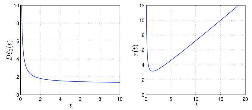
Figure 1: Positions of the singularity in the expression (38) (left panel), and the prefactor (39) (right panel) as functions of time. These functions control, through Eq. (40), the large $|w|$ asymptotics of the work PDF. In the right panel we have taken $D=1$ and $g=1$.

The asymptotics of the work PDF $p(w;t)$ for $w\!\to\!-\infty$ (at fixed $t$) is determined by the expansion of the characteristic function $\Phi(\xi;t)$ at that $\xi_{0}(t)$, which gives the singularity of $\Phi(\xi;t)$ lying closest to its domain of analyticity [22]. To find $\xi_{0}(t)$, we numerically solved the transcendental equation $1/\Phi(\xi_{0}(t);t)=0$. In the vicinity of the singularity,

$$\Phi(\xi;t)\sim r(t)\left(-\frac{1}{D(\xi-\xi_{0}(t))}\right)^{\nu+1}\,,\quad\xi\to\xi_{0}(t)\,\,,$$ (38)

with

$$r(t)=(-D)^{\nu+1}\!\!\lim_{\xi\to\xi_{0}(t)}\left(\xi-\xi_{0}(t)\right)^{\nu+1}\Phi(\xi;t)\,\,.$$ (39)

From this result we obtain [22]

$$p(w;t)\sim\frac{1}{D}\,\frac{r(t)}{\Gamma(\nu+1)}\left(\frac{|w|}{D}\right)^{\nu}{\rm e}^{-D\xi_{0}(t)\frac{|w|}{D}}\quad,\quad w\to-\infty\,\,,$$ (40)

where $D\xi_{0}(t)$ is a real, positive, decreasing function of $t$, cf. Fig. 1. For small $t$, the work PDF is very narrow ($D\xi_{0}(t)$ large). With increasing $t$, the weight of the trajectories yielding large (absolute) values of the work increases. This is reflected by the decrease of $D\xi_{0}(t)$. Contrary to the function $c_{2}(t)$ in (36), $D\xi_{0}(t)$ does not depend on the strength of the logarithmic potential. The parameter $g$ enters only the pre-exponential factor in Eq. (40).

In order to verify the exact asymptotic expansions of the work PDF, we have performed extensive Langevin dynamics simulations using the Heun algorithm [27] for several sets of parameters and different time intervals. A typical PDF together with the predictions for its asymptotic behavior according to Eqs. (36) and (40) is shown in Fig. 2. In order to avoid nonphysical negative values of the particle position in the numerics, which can originate from a fixed time discretization, we have implemented a time-adapted Heun scheme. If a negative (attempted) coordinate along a trajectory is generated, the time step $\Delta t$ is reduced until the attempted particle position is positive. To allow for a better comparison of the analytical findings with the simulated data in Fig. 2 for small $|w|$, we have derived also the second leading term in the asymptotic expansion for $|w|\to 0$. After somewhat lengthy but straightforward calculation, we obtain

$$p(w;t)\sim c_{1}(t)\left[\left(\frac{|w|}{D}\right)^{\nu-\frac{1}{2}}-\sqrt{\frac{4}{(\nu+1)\ln(1+t)}}\left(\frac{|w|}{D}\right)^{\nu+\frac{1}{2}}\right]{\rm e}^{-c_{2}(t)\frac{D}{|w|}}\,\,,\quad w\to 0^{-}\,\,,$$ (41)

where $c_{1}(t)$ and $c_{2}(t)$ are given in Eq. (37).

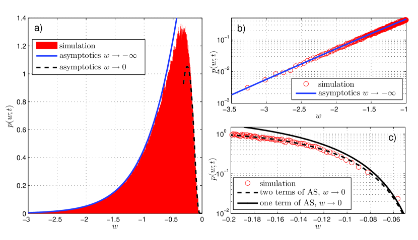
Figure 2: a) Simulated work PDF in comparison with the asymptotic behavior predicted by Eq. (40) ($|w|$ large, solid line) and Eq. (41) ($|w|$ small, dashed line) for parameters $g=1.5$, $D=1$ and $t=1$. In the simulations $10^{6}$ trajectories were generated with a time step $\Delta t=0.001$ (adapted when the particle is near the origin, see text). b) Semi-logarithmic plot of simulated $p(w;t)$ vs. $w$ (circles), demonstrating the agreement with Eq. (40) (solid line) for large $|w|$. c) Semi-logarithmic plot of simulated $p(w;t)$ vs. $w$ (circles) in comparison with the first leading term of the asymptotic expansion for small $|w|$ (Eq. (36), solid line), and when including the second leading term according to Eq. (41) (dashed line).

5 Concluding remarks

Based on a Lie algebraic approach we succeeded to derive Eq. (18) for the joint PDF of work and position for a Brownian particle in a time-dependent logarithmic-harmonic potential. In order to derive explicit results from Eq. (18) for a given protocol, the Riccati equation (16) needs to be solved. This nonlinear differential equation is equivalent to the linear second-order differential equation [28]

$$\ddot{y}(t)-2k(t)\dot{y}(t)-2D\xi\dot{k}(t)y(t)=0\quad,\quad\dot{y}(0)=0\,\,.$$ (42)

Specifically, if $y(t)$ solves (42), then the logarithmic derivative

$$b_{2}(t)=-\frac{2}{D}\frac{\dot{y}(t)}{y(t)}\,\,,$$ (43)

is the solution of Eq. (16). Hence the characteristic function (28) can be expressed in terms of the function $y(t)$.

The solution of (42) for several reasonable driving protocols, e.g., for $k(t)=k_{0}\exp(\pm\gamma t)$, $k(t)=k_{0}+k_{1}t$, or $k(t)=k_{1}t^{n}$, can be written in terms of higher transcendental functions. Corresponding results are quite involved and will be published elsewhere. Here we have focused on the simple protocol (29) which should exemplify typical asymptotic features of the work PDF for monotonic driving. Notice that, if $\dot{k}(t)>0$ and $\xi\to\infty$ along the real axis, one can use the WKB approximation and derive a generic expression for $y(t)$ valid for any protocol, i.e., also a generic approximative expression for the work characteristic function (28).

For non-monotonic driving protocols the work can assume any real value. Then the work PDF has the support $(-\infty,+\infty)$ and its two-sided Laplace transform will be analytic within a stripe parallel to the imaginary axis. The $w\to+\infty$ ($w\to-\infty$) tail of the work PDF is determined by the singularity, which is closest to the stripe on its left (right) side. We hence expect an asymptotics

$$p(w;t)\sim\frac{1}{D}\frac{r_{\pm}(t)}{\Gamma(\nu+1)}\left(\frac{|w|}{D}\right)^{\nu}{\rm e}^{-D\xi_{\pm}(t)\frac{|w|}{D}}\quad,\quad w\to\pm\infty\,\,,$$ (44)

where the coefficients $\xi_{\pm}(t)$, $r_{\pm}(t)$, depend on the driving protocol $k(t)$. Periodic driving protocols play an important role in the analysis of Brownian motors. A deeper analysis of the work PDF for this class of protocols seems to be worthy for further study.

References

References

- [1] U. Seifert, Stochastic thermodynamics: Principles and perspectives, Eur. Phys. J. B, 64:423, 2011.
- [2] M. Esposito and C. Van den Broeck, Three faces of the second law. I. Master equation formulation, Phys. Rev. E, 82:011143, 2010.
- [3] M. Esposito and C. Van den Broeck, Three faces of the second law. II. Fokker-Planck formulation, Phys. Rev. E, 82:011144, 2010.
- [4] C. Jarzynski, Nonequilibrium equality for free energy differences, Phys. Rev. Lett., 78:2690–2693, Apr 1997.
- [5] D. A. Kessler and E. Barkai, Infinite covariant density for diffusion in logarithmic potentials and optical lattices, Phys. Rev. Lett., 105:120602, 2010.
- [6] A. E. Cohen, Control of nanoparticles with arbitrary two-dimensional force fields, Phys. Rev. Lett., 94:118102, 2010.
- [7] V. Blickle and C. Bechinger, Realization of a micrometre-sized stochastic heat engine, Nat. Phys., 8:143, 2012.
- [8] J. A. Giampaoli et al., Exact expression for the diffusion propagator in a family of time-dependent anharmonic potentials, Phys. Rev. E, 60:2540, 1999.
- [9] J. Wei and E. Norman, Lie algebraic solution of linear differential equations, J. Math. Phys., 4:575, 1963.
- [10] F. Wolf, Lie algebraic solutions of linear Fokker-Planck equations, J. Math. Phys., 29:305, 1988.
- [11] A. Engel, Asymptotics of work distributions in nonequilibrium systems, Phys. Rev. E, 80:021120, 2009.
- [12] D. Nickelsen and A. Engel, Asymptotics of work distributions: the pre-exponential factor, Eur. Phys. J. B, 82:207, 2011.
- [13] T. Speck, Work distribution for the driven harmonic oscillator with time-dependent strength: Exact solution and slow driving, J. Phys. A: Math. Theor., 44:305001, 2011.
- [14] D. D. L. Minh and A. B. Adib, Path integral analysis of Jarzynski’s equality: Analytical results, Phys. Rev. E, 79:021122, 2009.
- [15] O. Mazonka and C. Jarzynski, Exactly solvable model illustrating far-from-equilibrium predictions, arXiv:cond-mat/9912121, 1999.
- [16] R. van Zon and E. G. D. Cohen, Stationary and transient work-fluctuation theorems for a dragged Brownian particle, Phys. Rev. E, 67:046102, 2003.
- [17] R. van Zon and E. G. D. Cohen, Extended heat-fluctuation theorems for a system with deterministic and stochastic forces, Phys. Rev. E, 69:056121, 2004.
- [18] E. G. D. Cohen, Properties of nonequilibrium steady states: a path integral approach, J. Stat Mech., page P07014, 2008.
- [19] S. Karlin and H. M. Taylor, A Second Course in Stochastic Processes, Academic Press, New York, 1981.
- [20] A. J. Bray, Random walks in logarithmic and power-law potentials, nonuniversal persistence, and vortex dynamics in the two-dimensional XY model, Phys. Rev. E, 62:103, 2000.
- [21] S. Redner, A Guide to First-Passage Processes, Cambridge University Press, 2001.
- [22] G. Doetsch, Introduction to the Theory and Application of The Laplace Transformation, Springer-Verlag, Berlin Heidelberg, 1974.
- [23] R. M. Wilcox, Exponential operators and parameter differentiation in quantum physics, J. Math. Phys., 8:962, 1967.
- [24] C. F. Lo, Exact propagator of the Fokker-Planck equation with logarithmic factors in diffusion and drift terms, Phys. Lett. A, 319:110, 2003.
- [25] H. Bateman and A. Erdélyi, Tables of Integral Transforms, volume 1, McGraw-Hill Book Company, INC., New York, 1954.
- [26] A. Erdélyi, editor, Higher Transcendental Functions, volume 2, Robert E. Krieger Publishing Company, INC., Malabar, Florida, 1955.
- [27] P. E. Kloeden and E. Platen, Numerical Solution of Stochastic Differential Equations, Springer-Verlag, Berlin, 1999.
- [28] A. D. Polyanin and V. F. Zaitsev, Handbook of Exact Solutions for Ordinary Differential Equations, Chapman & Hall/CRC, Boca Raton, 2-nd edition, 2003.