A symplectic integrator for the symmetry reduced and regularised planar 3–body problem with vanishing angular momentum

Abstract

We construct an explicit reversible symplectic integrator for the planar 3-body problem with zero angular momentum. We start with a Hamiltonian of the planar 3-body problem that is globally regularised and fully symmetry reduced. This Hamiltonian is a sum of 10 polynomials each of which can be integrated exactly, and hence a symplectic integrator is constructed. The performance of the integrator is examined with three numerical examples: The figure eight, the pythagorean orbit, and a periodic collision orbit.

Keywords: geometric integration explicit symplectic integration numerical integration 3-body problem symmetry reduction hamiltonian system regularisation

1 Introduction

It is well known that the flow $\Psi_{H}^{t}$ of a Hamiltonian $H$ of the form $H=T(p)+V(q)$ with conjugate variables $q$ and $p$ can be approximated by splitting it into the integrable flow $\Psi_{T}^{t}$ of $T(p)$ and the integrable flow $\Psi_{V}^{t}$ of $V(q)$ and observing that $\Psi_{H}^{t}=\Psi_{T}^{t}\circ\Psi_{V}^{t}+O(t^{2})$, see, e.g.  Channell and Neri (1996); Hairer et al (2002); McLachlan and Quispel (2002); Leimkuhler and Reich (2004). Thus a first order explicit symplectic integrator is obtained, and higher order methods can be constructed along similar lines Yoshida (1990). In an integrable and separable Hamiltonian system of the form $H=H_{1}(q_{1},p_{1})+H_{2}(q_{2},p_{2})$ such splitting gives the exact identity $\Psi_{H}^{t}=\Psi_{H_{1}}^{t}\circ\Psi_{H_{2}}^{t}$. If instead the Hamiltonian is a product $H=H_{1}(q_{1},p_{1})H_{2}(q_{2},p_{2})$ again the system is integrable with integrals $H_{1}$ and $H_{2}$ and the flow can be written as

$$\Psi_{H}^{t}=\Psi_{H_{1}}^{tH_{2}}\circ\Psi_{H_{2}}^{tH_{1}}=\Psi_{H_{2}}^{tH_{1}}\circ\Psi_{H_{1}}^{tH_{2}}\,.$$

In the superscript $tH_{i}$ denotes multiplication of $t$ by the (constant) value of $H_{i}$. A monomial Hamiltonian is a special case that has the same structure. There are obvious generalisations to more degrees of freedom. Hence any polynomial Hamiltonian is a sum of integrable monomial Hamiltonians, and thus a splitting integrator can be constructed. Symplectic integration of polynomial Hamiltonians has been discussed in Shi and Yan (1993); Gjaja (1994); Channell and Neri (1996); Blanes (2002); Quispel and Mclachlan (2004). In a recent paper by Blanes and Iserles (2012) various methods for time step control in geometric integrators are constructed and discussed. These methods could be useful in order to implement variable time stepping on top of our method, see the discussion in section 3.4.

In this paper we apply these methods to the polynomial Hamiltonian of the globally regularised and symmetry reduced 3-body problem at angular momentum zero. For a review of numerical and regularisation methods in the $n$-body problem we refer to Ito and Tanikawa (2007). It is well known that binary collisions in the 3-body problem can be regularised. Regularisation consists of a canonical transformations which essentially extracts a square root near collision, and of a scaling of time so that the approach to the collision is slowed down. The classical simultaneous regularisation of the (spatial) 3-body problem is due to Heggie (1974). This increases the dimension of phase space from 18 to 24. Instead we would like to decrease the dimension of phase space by using reduction at the same time as regularisation. The simultaneous regularisation of the planar 3-body problem is due to Lemaître (1964), and we use a version due to Waldvogel (1982). This is a symmetric simultaneous regularisation of the symmetry reduced planar 3-body problem and has the smallest possible 6-dimensional phase space. The resulting Hamiltonian is a polynomial of up to degree 6 in the canonical variables. A modern extension of these regularising transformations has recently been given by Moeckel and Montgomery (2012), however, their Hamiltonians are not polynomial but rational.

Our paper applies the methods for construction of an explicit symplectic integrator to Waldvogel’s Hamiltonian with angular momentum zero. We also describe how a similar integrator could be constructed for Heggie’s Hamiltonian, which works for non-zero angular momentum and in the spatial problem.

2 The 3-body Hamiltonian

The classical 3-body problem has long been studied, but still many open questions regarding its dynamics remain. For many questions, e.g. the study of relative periodic orbits, it is useful to reduce by translational and rotational symmetries, so that the absolute rotation of an orbit can be separated from shape dynamics in the centre of mass frame. Moreover, to study collision or near-collision orbits it is essential to perform (global) regularisation of the binary collisions. Following Waldvogel (1982) we are going to do both.

If the position and momentum of mass $m_{j}$, for $j=1,2,3$, are given by complex Cartesian coordinates $X_{j}$ and $P_{j}$ respectively, we can transform into symmetry-reduced coordinates such that

$$X_{l}-X_{k}=a_{j}e^{\phi_{j}},$$

where $a_{j}=|X_{l}-X_{k}|$ is the length of the triangle’s side opposite to $m_{j}$, $\phi_{j}$ is the angle of that side in the original coordinate system (in the direction of $m_{k}$ to $m_{l}$), as illustrated in figure 1, and $(j,k,l)$ represents cyclic permutations of $(1,2,3)$.

Figure 1: Coordinates of a triangle in the plane with centre of mass at the origin $O$.

This reduction results in coordinates $a_{j}$ and $\phi=\frac{1}{3}(\phi_{1}+\phi_{2}+\phi_{3})$, which represents the orientation angle of the triangle with respect to the original choice of Cartesian coordinates, and corresponding canonical momenta $p_{j}$ and $p_{\phi}$. The Hamiltonian rewritten in these coordinates is independent of $\phi$, so $p_{\phi}$ is a constant of motion. Hamilton’s equations for $(a_{j},\phi,p_{j},p_{\phi})$ give the reduced dynamics, including a differential equation for $\phi$ which may be integrated along to be able to recover the unreduced position of the triangle.

Figure 2: Physical significance of the regularised coordinates $\alpha_{j}$.

The globally regularising transformation, illustrated in figure 2, goes from symmetry-reduced to regularised coordinates, simultaneously regularising all the binary collisions. Define $\alpha_{j}$ for $j=1,2,3$ such that $a_{j}=\alpha_{k}^{2}+\alpha_{l}^{2}$. In this way $\alpha_{j}^{2}$ is the distance from $m_{j}$ to the point where the incircle of the triangle touches the sides adjacent to $m_{j}$.

The space of coordinates $(a_{j})$ is the space of all triangles, not accounting for orientation. Orientation is taken to be positive if, going clockwise around the triangle, the masses are encountered in a cyclic permutation of $(1,2,3)$ or negative otherwise. The space of all possible oriented triangles is called the shape space, and the space of $(\alpha_{j})$ is a four-fold covering of this space, in which the sign of the product $\alpha_{1}\alpha_{2}\alpha_{3}$ determines the orientation of the triangle. Thus the triangle formed by $(\alpha_{1},\alpha_{2},\alpha_{3})$ is the same as the ones formed by $(\alpha_{1},-\alpha_{2},-\alpha_{3})$, $(-\alpha_{1},\alpha_{2},-\alpha_{3})$ and $(-\alpha_{1},-\alpha_{2},\alpha_{3})$.

Canonically conjugate momenta $\pi_{j}$ are introduced using a generating function. Finally the time scaling

$$\frac{\text{d}t}{\text{d}\tau}=a_{1}a_{2}a_{3}$$ (1)

together with Poincaré’s trick to make this Hamiltonian yields the regularised and symmetry reduced polynomial Hamiltonian

$$K=(H-h)a_{1}a_{2}a_{3},$$

where $H$ is the original Hamiltonian written in the new coordinates and $h=H(\boldsymbol{\alpha}_{0},\boldsymbol{\pi}_{0})$ is the energy corresponding to the initial conditions $(\boldsymbol{\alpha}_{0},\boldsymbol{\pi}_{0})$, so only those solutions for which $K\equiv 0$ are physically meaningful.

The Hamiltonian of the zero-angular momentum 3-body problem in regularised coordinates is

$$K=K_{0}-ha_{1}a_{2}a_{3},$$ (2)

where

$$K_{0}=\frac{1}{8}\boldsymbol{\pi}^{T}B(\boldsymbol{\alpha})\boldsymbol{\pi}-\sum m_{k}m_{l}a_{k}a_{l},$$ (3)

in which

$$\boldsymbol{\pi} =\begin{pmatrix}\pi_{1}&\pi_{2}&\pi_{3}\end{pmatrix}^{T}$$

$$\boldsymbol{\alpha} =\begin{pmatrix}\alpha_{1}&\alpha_{2}&\alpha_{3}\end{pmatrix}^{T}$$

$$B(\boldsymbol{\alpha}) =\begin{pmatrix}A_{1}&B_{3}&B_{2}\\ B_{3}&A_{2}&B_{1}\\ B_{2}&B_{1}&A_{3}\end{pmatrix},$$

where

$$A_{j} =\dfrac{a_{j}}{m_{j}}\alpha^{2}+\dfrac{a_{k}}{m_{k}}\alpha_{l}^{2}+\dfrac{a_{l}}{m_{l}}\alpha_{k}^{2},$$

$$B_{j} =-\dfrac{a_{j}}{m_{j}}\alpha_{k}\alpha_{l}\text{\ \ and}$$

$$\alpha^{2} =\alpha_{1}^{2}+\alpha_{2}^{2}+\alpha_{3}^{2}.$$

The sum in (3) (and any hereafter where the index of summation is unspecified) is over cyclic permutations of $(1,2,3)$, so that $(j,k,l)$ is replaced by $(1,2,3)$, $(2,3,1)$, and $(3,1,2)$ in turn, and then the three corresponding terms are added together. When there is no summation the indices $(j,k,l)$ take on the three possible cyclic permutations in turn, as, e.g., in the definition of $A_{j}$ and $B_{k}$ above.

The new Hamiltonian is a polynomial in $\boldsymbol{\alpha}$ and $\boldsymbol{\pi}$, and thus Hamilton’s equations of motion for this system can be integrated with an explicit symplectic integrator obtained by splitting into monomials. As we are going to show in the next section it is more efficient to split into certain polynomials whose flow can be exactly solved.

3 Construction of the Symplectic Integrator

The basic building blocks of the integrator are the exact solutions for monomial Hamiltonians $H_{mn}=q^{m}p^{n}$ in one degree of freedom. The flow of this Hamiltonian for $m\neq n$ is

$$\psi_{mn}^{t}(q,p)=(q\beta^{n},p\beta^{-m}),\quad\mbox{ where }\quad\beta=\left(1+(n-m)q^{m-1}p^{n-1}t\right)^{\frac{1}{n-m}}$$ (4)

while for $m=n$ it is

$$\psi_{m}^{t}(q,p)=(q\beta,p/\beta),\quad\mbox{ where }\quad\beta=\exp(m(qp)^{m-1}t)\,.$$ (5)

For the Hamiltonian we are studying the cases that occur are $n=m=1$, $n=m=2$, and $m=3$, $n=1$. We also recall that if the Hamiltonian is a function of positions or momenta only (with any number of degrees of freedom) the flows are

$$\psi_{T(p)}^{t}(q,p)=(q+(\nabla_{p}T)t,p),\quad\mbox{ and }\quad\psi_{U(q)}^{t}(q,p)=(q,p-(\nabla_{q}U)t)\,.$$ (6)

3.1 Integrable Polynomial Hamiltonians

The basic building blocks just mentioned are now combined to form integrators for the terms that appear in the Hamiltonian $K$. The main observation is that if the Hamiltonian is a product of factors that depend on disjoint groups of degrees of freedom, then each factor is a constant of motion. Each of the factors in our case is either depending on momenta or positions only (denoted by $T(p)$ or $U(q)$) or it is a single monomial in one degree of freedom (denoted by $H_{mn})$ or a sum of monomials of disjoint degrees of freedom (denoted by $G$).

We now list the cases that are relevant in our case (recall that each of the factors depends on disjoint groups of degrees of freedom):

$$H_{a}=TH_{nm},\quad \psi_{a}=\psi_{T}^{tH_{nm}}\circ\psi_{nm}^{tT}$$ (7a)

$$H_{b}=TV,\quad \psi_{b}=\psi_{T}^{tV}\circ\psi_{V}^{tT}$$ (7b)

$$H_{c}=GH_{nm},\quad \psi_{c}=\psi_{nm}^{tG}\circ\psi_{G}^{tH_{nm}}$$ (7c)

where $G$ is a Hamiltonian which is the sum of Hamiltonians depending on disjoint degrees of freedom $G=H_{1}(q_{1},p_{1})+H_{2}(q_{2},p_{2})$ and thus $\psi_{G}=\psi_{H_{1}}\circ\psi_{H_{2}}$. Note that all these formulas are exact, and that the order of composition is irrelevant since the flows commute and the individual factors are constants of motion.

3.2 Splitting

Let us now explain how to split $K$ (2) into such terms. It is a polynomial Hamiltonian of degree $6$ in $\boldsymbol{\alpha}$ and $\boldsymbol{\pi}$ with 34 monomials. There are $13$ monomials, dependent only on $\boldsymbol{\alpha}$, of degrees $6$ and $4$, which may be treated as a single stage. The remaining $21$ terms may be grouped such that only $9$ more stages are necessary to approximate the flow of the full Hamiltonian to first order in the time step in $10$ stages. Let $K=\sum_{i=0}^{9}H_{i}$, where we set $M_{j}=m_{k}m_{l}$ and $N_{j}=\frac{1}{m_{k}}+\frac{1}{m_{l}}$. Then the splitting is

$$\begin{array}[]{rlrl}H_{0}=&-\sum M_{j}\alpha_{j}^{4}-\left(\sum M_{j}\right)\left(\sum\alpha_{k}^{2}\alpha_{l}^{2}\right)-ha_{1}a_{2}a_{3}&=&\ \ \ \ \ C_{0}\\ H_{1}=&\frac{1}{8}\left(N_{2}\alpha_{2}^{2}+N_{3}\alpha_{3}^{2}\right)\alpha_{1}^{2}\pi_{1}^{2}&=&\ \ \frac{1}{8}\ C_{1,23}\ C_{1,1}\\ H_{2}=&\frac{1}{8}\left(N_{3}\alpha_{3}^{2}+N_{1}\alpha_{1}^{2}\right)\alpha_{2}^{2}\pi_{2}^{2}&=&\ \ \frac{1}{8}\ C_{2,31}\ C_{2,2}\\ H_{3}=&\frac{1}{8}\left(N_{1}\alpha_{1}^{2}+N_{2}\alpha_{2}^{2}\right)\alpha_{3}^{2}\pi_{3}^{2}&=&\ \ \frac{1}{8}\ C_{3,12}\ C_{3,3}\\ H_{4}=&\frac{1}{8}\left(N_{2}\alpha_{2}^{4}+\frac{2}{m_{1}}\alpha_{2}^{2}\alpha_{3}^{2}+N_{3}\alpha_{3}^{4}\right)\pi_{1}^{2}&=&\ \ \frac{1}{8}\ C_{4}\\ H_{5}=&\frac{1}{8}\left(N_{3}\alpha_{3}^{4}+\frac{2}{m_{2}}\alpha_{3}^{2}\alpha_{1}^{2}+N_{1}\alpha_{1}^{4}\right)\pi_{2}^{2}&=&\ \ \frac{1}{8}\ C_{5}\\ H_{6}=&\frac{1}{8}\left(N_{1}\alpha_{1}^{4}+\frac{2}{m_{3}}\alpha_{1}^{2}\alpha_{2}^{2}+N_{2}\alpha_{2}^{4}\right)\pi_{3}^{2}&=&\ \ \frac{1}{8}\ C_{6}\\ H_{7}=&-\frac{1}{4}\left(\frac{1}{m_{3}}\alpha_{2}\pi_{2}+\frac{1}{m_{2}}\alpha_{3}\pi_{3}\right)\alpha_{1}^{3}\pi_{1}&=&-\frac{1}{4}\ C_{7,23}\ C_{7,1}\\ H_{8}=&-\frac{1}{4}\left(\frac{1}{m_{1}}\alpha_{3}\pi_{3}+\frac{1}{m_{3}}\alpha_{1}\pi_{1}\right)\alpha_{2}^{3}\pi_{2}&=&-\frac{1}{4}\ C_{8,31}\ C_{8,2}\\ H_{9}=&-\frac{1}{4}\left(\frac{1}{m_{2}}\alpha_{1}\pi_{1}+\frac{1}{m_{1}}\alpha_{2}\pi_{2}\right)\alpha_{3}^{3}\pi_{3}&=&-\frac{1}{4}\ C_{9,12}\ C_{9,3},\end{array}$$ (8)

where each subindexed function $C_{i}$ is a constant of motion in its associated Hamiltonian.

There are clearly four groups in equation (8), which we shall enumerate 0: {0}, 1: {1,2,3}, 2: {4,5,6} and 3: {7,8,9}. $H_{0}$ depends on coordinates only, so can be integrated by (6). Group 1 can be integrated by (7b), group 2 can be integrated by (7a), and finally group 3 can be integrated by (7c) where $G$ is a sum of $H_{mm}$ Hamiltonians.

3.3 Higher order methods

An important ingredient in constructing higher order reversible methods is the adjoint $(\phi^{t})^{*}$ of a method $\phi^{t}$ which is defined to be $(\phi^{-t})^{-1}$. If $\phi^{t}=\psi_{1}^{t}\circ\psi_{2}^{t}\circ\dots\circ\psi_{n}^{t}$ and each $\psi_{i}^{t}$ is self-adjoint, then the adjoint is obtained by reversing the order of composition. This follows from the definition of the adjoint:

$$(\phi^{t})^{*} =(\phi^{-t})^{-1}$$

$$=(\psi_{1}^{-t}\circ\psi_{2}^{-t}\circ\dots\circ\psi_{n}^{-t})^{-1}$$

$$=(\psi_{n}^{-t})^{-1}\circ(\psi_{n-1}^{-t})^{-1}\circ\dots\circ(\psi_{1}^{-t})^{-1}$$

$$=\psi_{n}^{t}\circ\psi_{n-1}^{t}\circ\dots\circ\psi_{1}^{t}\,.$$

In our case the self-adjointness of the individual steps $\psi_{i}^{t}$ follows from the fact that they are exact solution of Hamilton’s equations.

Channell & Neri Channell and Neri (1996) offer a basic derivation of a reversible, symplectic map that is accurate to second order in the time step. When the splitting is of the form $H=T(p)+U(q)$ this leads to the symplectic leapfrog integrator, by composing symplectic Euler with its adjoint.

This construction also applies to the more complicated case with a first order integrator composed of 10 self-adjoint maps as in our case. Given $\phi^{t}=\psi_{1}^{t}\circ\psi_{2}^{t}\circ\dots\circ\psi_{n}^{t}$ as above a reversible second order method is found as

$$\phi_{2}^{t} =\phi_{1}^{\frac{t}{2}}\circ(\phi_{1}^{\frac{t}{2}})^{*}$$

$$=\psi_{1}^{\frac{t}{2}}\circ\dots\circ\psi_{n-1}^{\frac{t}{2}}\circ\psi_{n}^{t}\circ\psi_{n-1}^{\frac{t}{2}}\circ\dots\circ\psi_{1}^{\frac{t}{2}}.$$

Yoshida (1990) gives a general method by which one may obtain integrators of arbitrary even order, if only one has, to start with, a reversible even-order integrator $\phi_{2}^{t}$ such as the symplectic leapfrog—or, more generally, symplectic midpoint. One can compose $\phi_{2}^{t}$ to obtain a fourth order integrator $\phi_{4}^{t}$, and compose this to obtain $\phi_{6}^{t}$ and so on. In general, given $\phi_{2n}^{t}$,

$$\phi_{2n+2}^{t}=\phi_{2n}^{z_{1}t}\ \phi_{2n}^{z_{0}t}\ \phi_{2n}^{z_{1}t},$$ (9)

where we define $z_{0}=-\dfrac{2^{1/(2n+1)}}{2-2^{1/(2(2n+1))}},z_{1}=\dfrac{1}{2-2^{1/(2n+1)}}$ to adjust the step size of the lower order method.

This method is easy to construct and implement, but quickly becomes unwieldy. When $n=2$ (order $4$), there are three evaluations of the second order method, but at orders $6$ and $8$ there are, respectively, nine and twenty-seven. As noted by Yoshida (1990), there are better methods, and he gives coefficients for a sixth order method and several sets of coefficients for eighth order methods. The construction of higher order methods is discussed extensively in Hairer et al (2002) and McLachlan and Quispel (2002). We will assess in section 4 which methods give good results for our problem comparing the methods whose coefficients are given in Hairer et al (2002) and those constructed by Yoshida (1990).

3.4 Regularisation and variable time stepping

There is a well known restriction on symplectic integration that such integrators must use a constant step size, or the benefits of these methods for large integration times are lost due to the introduction of new secular error terms. Various authors have discussed methods of achieving adaptive step size in symplectic integration that avoids this problem; for example, Mikkola (1997); Preto and Tremaine (1999); Blanes and Budd (2005); Blanes and Iserles (2012).

In particular, Blanes and Iserles (2012) explore the use of Sundman and Poincaré transformations and give a good overview of the problem. In general the Sundman transformation is non-symplectic, though with care the transformation can be made to respect geometric structure. In the their framework, the time scaling $\frac{\text{d}t}{\text{d}\tau}=a_{1}a_{2}a_{3}$ is called the monitor function. Our situation is special because the regularisation transformation consists of two intimately related steps. First there is the canonical extension of the transformation of coordinates from distances $a_{j}$ to their “roots” $\alpha_{j}$ (space regularisation), and second there is the time scaling (time regularisation). The time scaling up to a constant factor is achieved using the square of the Jacobian determinant of the transformation of the coordinates. Only the combination of the two achieves global regularisation. Treating the time transformation separately as a monitor function would mean to integrate singular equations, since the original equations are singular at collision, and they are still singular after the spatial regularisation alone. Slight modifications of the time scaling are possible, see the remark at the end of the next section.

In order to achieve variable time stepping a monitor function could be used in the way described by Blanes and Iserles (2012) by integrating another equation on top of the regularisation (in space and time) we have done. This may be particularly useful when integrating orbits with large distances between the bodies.

3.5 Finite time blowup

It must be noted that the solution of the Hamiltonian $H=q^{m}p^{n}$ given in (4) can (for $n\neq m$) reach infinity in finite time. This occurs when

$$1+(n-m)\ q_{0}^{m-1}\ p_{0}^{n-1}t=0.\$$ (10)

This obviously makes step sizes comparable to this threshold risky when this form of solution is used in the integrator. This singularity could be reached if the denominator is negative and large during forward timesteps, or if the denominator is positive and large for “backward” timesteps (as during the middle stage of Yoshida’s trick). This possibility arises in equation (2) in the group 4 of the splitting (8), which have terms of the form $\alpha_{j}^{3}\pi_{j}^{1}$. It may appear that this finite time blowup is an artefact of the integrator. However, after the time scaling the Hamiltonian $K$ does have finite time blow up when particles escape to infinity. In this light it seems less unexpected that a stage of the corresponding symplectic integrator shows the same behaviour.

Blanes (2002) provides a means by which to avoid such singularities, by way of rewriting the polynomial in terms of sums of binomials in the coordinates and momenta and finding coefficients such that the two expressions are equal. We did apply this to the Hamiltonian $H_{31}$ in our problem, and found a way to replace this with a Cremona map. However, it turned out that the overall error of the method was worse than without this modification. Our method is more expensive, since it needs to compute rational powers, but this additional cost is worth it.

A way to possibly avoid finite time blowup when the configuration of the system becomes large would be to consider a rational—rather than polynomial—time scaling function as in Moeckel and Montgomery (2012). One could consider, for example, $\frac{\text{d}t}{\text{d}\tau}=\frac{a_{1}a_{2}a_{3}}{\alpha^{2\gamma}}$ (recalling $\alpha^{2}=\sum\alpha_{j}^{2}$), which tends to $0$ for $\gamma=3$ or to ${a_{j}}/{4}$ for $\gamma=2$ as $\alpha_{j}\rightarrow\infty$. For negative energy, the only possible escape to infinity is of one single mass and a hard binary; in regularised coordinates this is exactly one coordinate tending to infinity while the other two remain bounded. Such a time scaling would inevitably require that the Hamiltonian be split differently, possibly with more stages and complexity. In principle the methods described in this paper apply as long as exact solutions can be found for the partial Hamiltonians. Unfortunately we have not been able to solve all of the resulting rational Hamiltonians.

3.6 Other polynomial globally regularised Hamiltonians

Our main concern in this paper is the zero-angular momentum reduced and regularised planar 3-body problem, which has 3 degrees of freedom. Other well known globally regularised polynomial Hamiltonians are due to Waldvogel (1972) for the planar 3-body problem and to Heggie (1974) for the spatial 3-body problem. These Hamiltonians are not fully symmetry reduced and have 4 degrees of freedom (planar arbitrary angular momentum) and 12 degrees of freedom (spatial arbitrary angular momentum).

Heggie’s simultaneously regularised Hamiltonian for the spatial 3-body problem Heggie (1974) in canonical variables $Q_{ji}$ and conjugate $P_{ji}$, $j=1,2,3$, $i=1,\dots,4$ has the form

$$H =H_{0}+H_{4}+H_{5}+H_{6}+H_{-1}$$

$$H_{0} =-ha_{1}a_{2}a_{3}-\sum m_{j}m_{k}a_{j}a_{k},$$

$$H_{3+l} =\frac{1}{8}\frac{a_{j}a_{k}}{\mu_{jk}}|p_{l}|^{2},\quad l=1,2,3$$

$$H_{-1} =\frac{1}{4}\sum\frac{a_{j}}{m_{j}}(A_{k}P_{k})\cdot(A_{l}P_{l})$$

where $\mu_{jk}=m_{j}m_{k}/(m_{j}+m_{k})$, and $a_{j}=\sum_{i=1}^{4}Q_{ji}^{2}$, $|p_{j}|^{2}=\sum_{i=1}^{4}P_{ji}^{2}$. In addition $P_{l}=(P_{l1},P_{l2},P_{l3},P_{l4})^{T}$ and $A_{l}$ is the KS-matrix Kustaanheimo and Stiefel (1965) of the form

$$A_{l}=\begin{pmatrix}Q_{l1}&-Q_{l2}&-Q_{l3}&Q_{l4}\\ Q_{l2}&Q_{l1}&-Q_{l4}&-Q_{l3}\\ Q_{l3}&Q_{l4}&Q_{l1}&Q_{l2}\\ \end{pmatrix}$$

The terms $H_{0}$ and $H_{4,5,6}$ are analogous to the previous ones. The terms in $H_{-1}$ can be split into 9 terms of the form $a_{j}f_{k}g_{l}$ where the functions $f_{k}$ and $g_{l}$ only depend on the degrees of freedom $k$ and $l$, respectively. These terms are somewhat similar to the Hamiltonians $H_{1,2,3}$ in Waldvogel’s case. Thus the Hamiltonian can be split into 13 polynomials of degree up to 6 each of which is integrable.

When setting $Q_{ji}$ and $P_{ji}$ with $i=3,4$ equal to zero Heggie’s Hamiltonian describes a planar problem. However, this still has 6 degrees of freedom. We can reduce the number of degrees of freedom to 4 by instead using Waldvogel’s Hamiltonian Waldvogel (1972); Gruntz and Waldvogel (2004). This Hamiltonian is a polynomial of degree 12 and can be split into 15 terms in a way similar to the two cases discussed above.

4 Numerical examples

In this section we will show some numerical results achieved using our integrator in a selection of orbits ranging from far from collision to close encounters to a collision orbit.

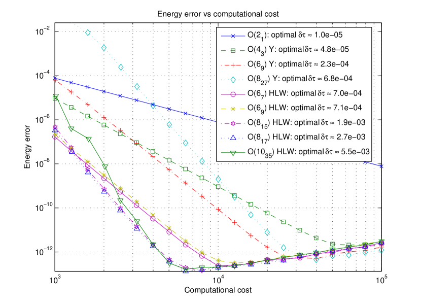
Figure 3: Averaged error, integrating a fixed time interval for varying integration costs. Time step size at the minimal error is listed for each order, as well as our source for the method.

Figure 3 shows the energy error for various integration methods in a “work-precision” diagram. The error is averaged over several different initial conditions integrated over a fixed time interval. The error is displayed as a function of the computational cost. The methods compared are the base method of order $2_{1}$, the integrators of Yoshida (1990) ($4_{3}$, $6_{9}$, and $8_{27}$) and other higher order symmetric compositions of symmetric methods of various authors, whose coefficients are given in Hairer et al (2002), section V.3.2, also see the references therein. The subscript with each method’s order indicates the number of second order substeps in the evaluation of a single time step, indicating the cost of each method, where the second order method is given the base cost of 1. A close look at the graph reveals that integrator $8_{17}$ achieves the lowest error with a step size of about $0.0027$, though it is a close call between any of the three best methods $8_{15}$, $8_{17}$ and $10_{35}$. Reducing the step size further creates larger round-off errors. All of the following examples are calculated with the $8_{17}$ integrator and step size $0.0027$, unless otherwise mentioned.

Consider the figure–8 choreography, discovered by Moore (1993), proved to exist by Chenciner and Montgomery (2000) and explored by Simó (2002, 2001). We choose initial conditions

$$\boldsymbol{\alpha}_{0} =(0,1.134522804969261,1.134522804969261)^{T}$$

$$\boldsymbol{\pi}_{0} =(1.506773685132772,0.694233777317562,-0.694233777317562)^{T}$$

in regularised coordinates, with $h=-1$ and equal unit masses. In scaled time, the figure-8 has a period of $2{.}221813718$; in physical time its period is $9.2371333$. The trajectory in regularised coordinates is shown in figures 4(a) and 4(b) and the energy error over 25 orbits with large time steps given by the period divided by 200 is shown in figure 4(c). Figure 5 shows the trajectory of this orbit in the 3-dimensional space $(\alpha_{j})$. Note that each crossing of a plane $\alpha_{j}=0$ corresponds to a syzygy with $m_{j}$ in the middle of the configuration.

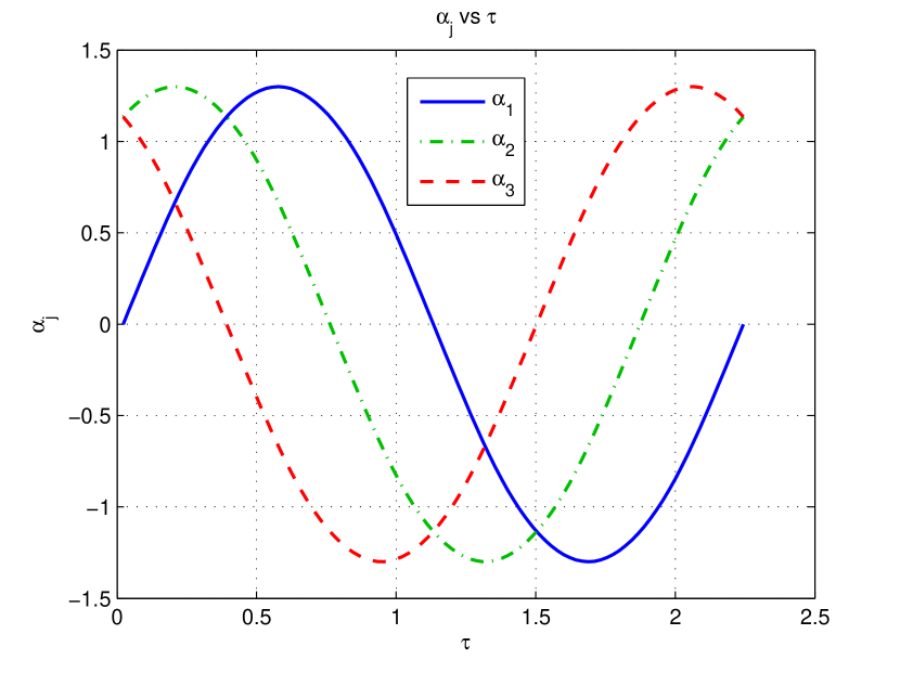
(a) Regularised coordinates.

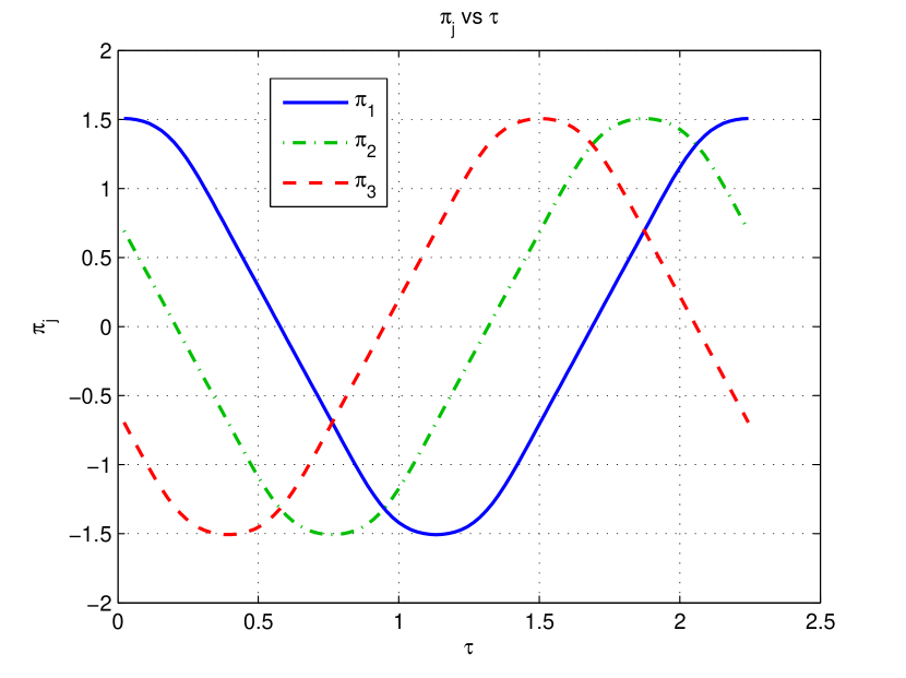
(b) Regularised momenta.

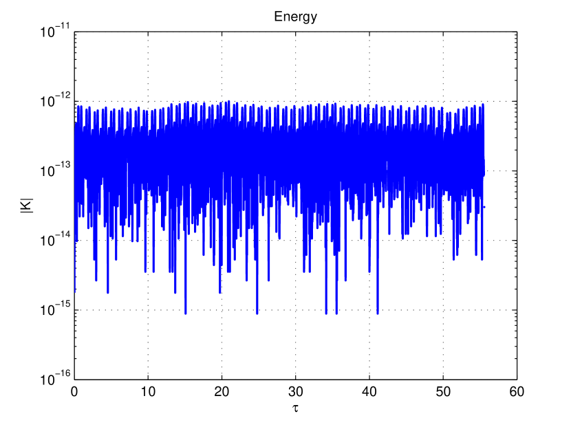
(c) Energy error for 25 periods with 200 time steps per period.

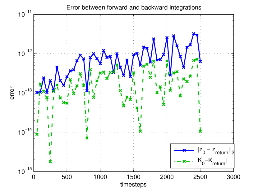
(d) Two-way integration error over 25 periods.

Figure 4: The figure–8 choreography with scaled period $2{.}221813718$.

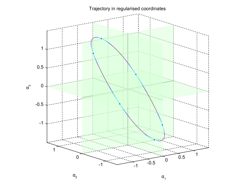
Figure 5: Trajectory of figure—8 choreography in $\alpha$-space, lying nearly in a plane. Colour gradient represents the moment of intertia (lighter is higher).

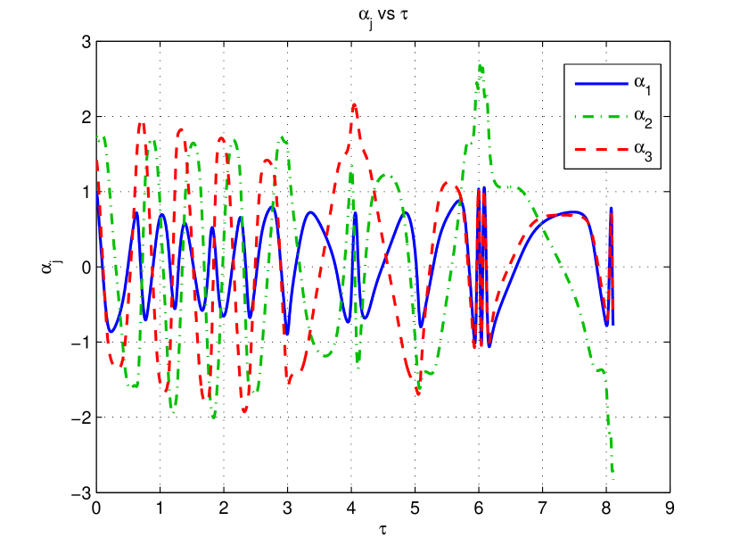
(a) Regularised coordinates.

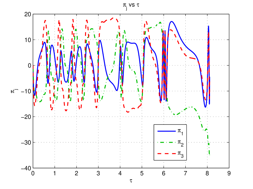
(b) Regularised momenta.

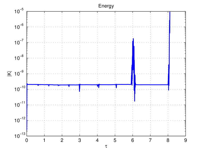
(c) Energy error.

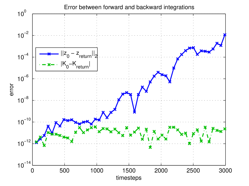
(d) Two-way integration error.

Figure 6: The Pythagorean orbit integrated up to $\tau=8{.}105$ in scaled time.

Next we look at the Pythagorean orbit Szebehely and Peters (1967) for $m_{1}=3$, $m_{2}=4$, $m_{3}=5$, with initial conditions as given in Gruntz and Waldvogel (2004), which, in regularised coordinates, are

$$\boldsymbol{\alpha}_{0} =(1,\sqrt{3},\sqrt{2})^{T}$$

$$\boldsymbol{\pi}_{0} =(0,0,0)^{T}.$$

This orbit has a close encounter between masses 1 and 3 at around $t=15.8$ in physical time (about $\tau=1.52$ in scaled time). Waldvogel’s analysis regularises the system, albeit slightly differently, and his integration is not symplectic. The final motions of this orbit compare well with other studies; plotting the orbit in physical space produces results indistinguishable from Szebehely and Peters (1967), Gruntz and Waldvogel (2004).

The regularisation of the 3—body problem allows our integrator to cope well when the distances between any two masses are small. The result of the time scaling is that the regularised system has a finite time blowup for any escape orbit. If one continues to integrate the Pythagorean orbit past $\tau=8.105$, the error in the energy grows exponentially and the results become inaccurate.

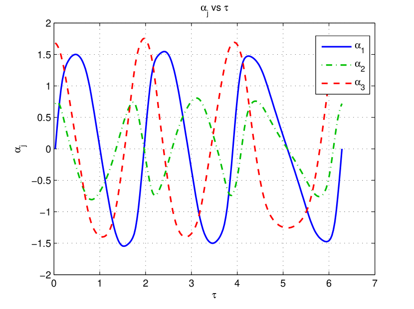
(a) Regularised coordinates.

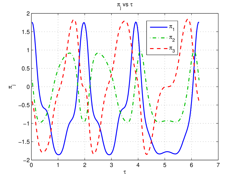
(b) Regularised momenta.

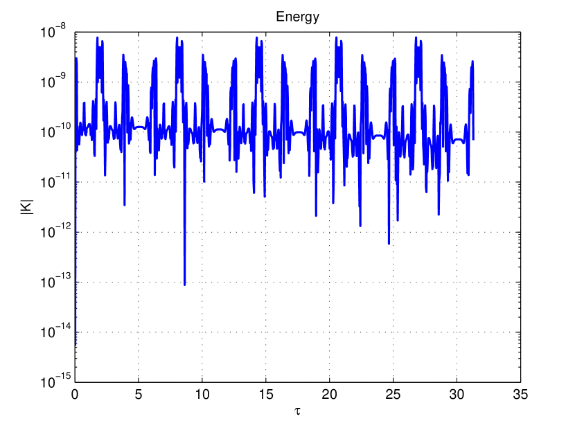
(c) Energy error for 5 periods.

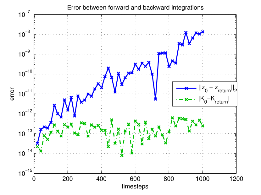
(d) Two-way integration error for 5 periods.

Figure 7: A periodic collision orbit with scaled period $6{.}2520511$ with 200 time steps per period.

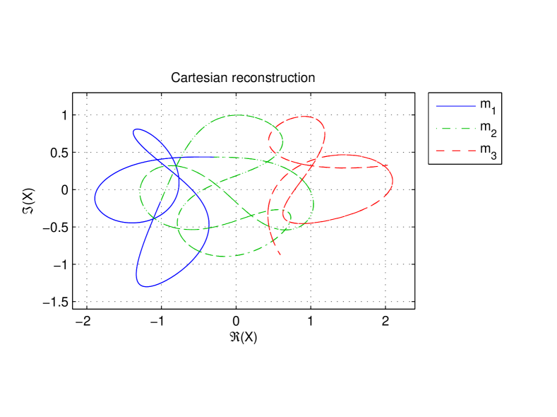
Figure 8: Reconstruction of Cartesian trajectories from regularised integration for a periodic collision orbit.

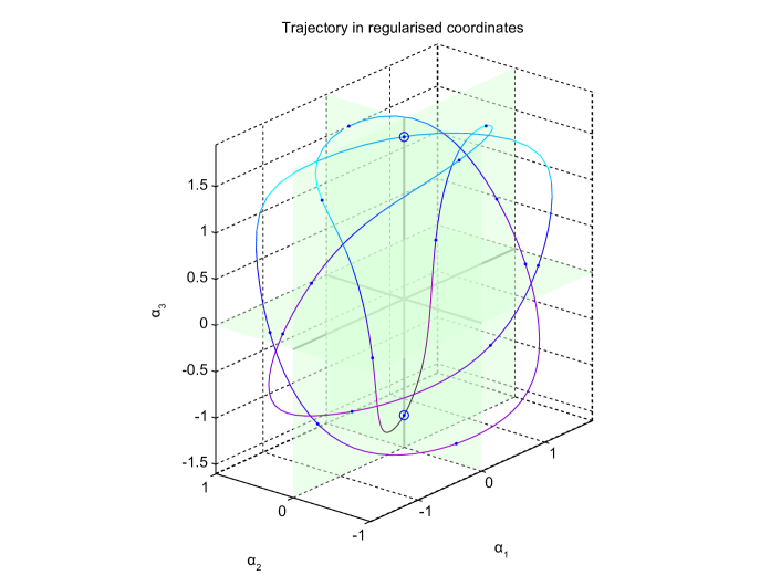
Figure 9: Trajectory of periodic collision orbit in $\alpha$-space. Colour gradient represents the moment of intertia of the configuration (lighter is higher). The two big dots mark the (regularised) collisions.

Finally, we show results in a periodic collision orbit, discovered during a search for periodic orbits in the reduced space, with initial conditions

$$\boldsymbol{\alpha}_{0} =(0,0.717162073833634,1.683647749751810)^{T}$$

$$\boldsymbol{\pi}_{0} =(1.762174970761679,0.177158588505747,-0.401743282150556)^{T},$$

equal unit masses and $h=-1$. This orbit has two collisions between masses 1 and 2, as can be seen by $\alpha_{1}=\alpha_{2}=0$ at $\tau=1.9362$ and $\tau=5.062$ in figure 7(a). This orbit is periodic in full phase space and is shown in figures 7, 8 and 9. Its scaled period is $6.2520511$, corresponding to a physical period of $29.6117209$. Note in figure 9 that the collisions happen on the $\alpha_{3}$-axis, when $\alpha_{1}=\alpha_{2}=0$.

Because Hamiltonian systems are time-reversible, it is desirable to have an integrator with the same property. The second order map $\phi_{2}^{t}$ is constructed as such, and Yoshida’s formula for higher order integrators constructs them to be reversible as well. That means that $\phi_{2n}^{t}\ \phi_{2n}^{-t}=Id$ up to roundoff error. Figures 4(d), 6(d) and 7(d) show how closely this integrator returns to its initial condition after a certain number of time steps in one direction, followed by the same number of iterations with a negative time step.

By this measure, the integrator has the most trouble with Pythagorean orbit, which clearly shows signs that it exists within a chaotic region of phase space by the exponential growth of error. However; energy is well preserved in this and the other cases.

5 Conclusion

We have constructed a symplectic integrator for the reduced and regularised planar 3-body problem at zero angular momentum. The method works well, but it is not very efficient, because each (first order) time step involves the computation of 10 individual maps. Our interests is the computation of relative periodic orbits including collision orbits, and for this task the method is appropriate. The detailed results about relative periodic orbits and their geometric phase will be reported in a forthcoming paper.

Appendix A Integrator stages

Subsection 3.1 described how to integrate a monomial Hamiltonian, and subsection 3.2 described the splitting of equation (2) into a minimal number of solvable parts and those solutions. Here we use those solutions to build an explicit first order symplectic composition method for (2).

Let the timestep be $\Delta\tau$, let $\mu_{j}=(m_{k}+m_{l})$, let the values of the system before and after one timestep respectively be $\boldsymbol{z}_{0}=(\alpha_{1,0},\dots,\pi_{3,0})^{T}$ and $\boldsymbol{z}_{1}=(\alpha_{1,1},\dots,\pi_{3,1})^{T}$ and intermediate steps be $\boldsymbol{\xi}_{i}=(\alpha_{1,.i-1},\dots,\pi_{3,.i-1})^{T}$. Now

$$\boldsymbol{\xi}_{1}= \begin{pmatrix}\alpha_{1,0}\\ \alpha_{2,0}\\ \alpha_{3,0}\\ \pi_{1,0}+2\alpha_{1,0}\left(\left(2\alpha_{1,0}^{2}+a_{1,0}\right)\left(ha_{1,0}+M_{1}\right)+m_{1}\alpha_{1,0}\mu_{1}a_{1,0}\right)\Delta\tau\\ \pi_{2,0}+2\alpha_{2,0}\left(\left(2\alpha_{2,0}^{2}+a_{2,0}\right)\left(ha_{2,0}+M_{2}\right)+m_{2}\alpha_{2,0}\mu_{2}a_{2,0}\right)\Delta\tau\\ \pi_{3,0}+2\alpha_{3,0}\left(\left(2\alpha_{3,0}^{2}+a_{3,0}\right)\left(ha_{3,0}+M_{3}\right)+m_{3}\alpha_{3,0}\mu_{3}a_{3,0}\right)\Delta\tau\end{pmatrix}$$

$$\boldsymbol{\xi}_{2}= \begin{pmatrix}\alpha_{1,.1}\ \exp\left(\frac{1}{4}\left(N_{2}\alpha_{2,.1}^{2}+N_{3}\alpha_{3,.1}^{2}\right)\alpha_{1,.1}\ \pi_{1,.1}\ \Delta\tau\right)\\ \alpha_{2,.1}\\ \alpha_{3,.1}\\ \pi_{1,.1}\ \exp\left(-\frac{1}{4}\left(N_{2}\alpha_{2,.1}^{2}+N_{3}\alpha_{3,.1}^{2}\right)\alpha_{1,.1}\ \pi_{1,.1}\ \Delta\tau\right)\\ \pi_{2,.1}-\frac{1}{4}\ N_{2}\ \alpha_{1,.1}^{2}\ \pi_{1,.1}^{2}\ \alpha_{2,.1}\Delta\tau\\ \pi_{3,.1}-\frac{1}{4}\ N_{3}\ \alpha_{1,.1}^{2}\ \pi_{1,.1}^{2}\ \alpha_{3,.1}\Delta\tau\end{pmatrix}$$

$$\boldsymbol{\xi}_{3}= \begin{pmatrix}\alpha_{1,.2}\\ \alpha_{2,.2}\ \exp\left(\frac{1}{4}\left(N_{3}\alpha_{3,.2}^{2}+N_{1}\alpha_{1,.2}^{2}\right)\alpha_{2,.2}\ \pi_{2,.2}\ \Delta\tau\right)\\ \alpha_{3,.2}\\ \pi_{1,.2}-\frac{1}{4}\ N_{1}\ \alpha_{2,.2}^{2}\ \pi_{2,.2}^{2}\ \alpha_{1,.2}\Delta\tau\\ \pi_{2,.2}\ \exp\left(-\frac{1}{4}\left(N_{3}\alpha_{3,.2}^{2}+N_{1}\alpha_{1,.2}^{2}\right)\alpha_{2,.2}\ \pi_{2,.2}\ \Delta\tau\right)\\ \pi_{3,.2}-\frac{1}{4}\ N_{3}\ \alpha_{2,.2}^{2}\ \pi_{2,.2}^{2}\ \alpha_{3,.2}\Delta\tau\end{pmatrix}$$

$$\boldsymbol{\xi}_{4}= \begin{pmatrix}\alpha_{1,.3}\\ \alpha_{2,.3}\\ \alpha_{3,.3}\ \exp\left(\frac{1}{4}\left(N_{1}\alpha_{1,.3}^{2}+N_{2}\alpha_{2,.3}^{2}\right)\alpha_{3,.3}\ \pi_{3,.3}\ \Delta\tau\right)\\ \pi_{1,.3}-\frac{1}{4}\ N_{1}\ \alpha_{3,.3}^{2}\ \pi_{3,.3}^{2}\ \alpha_{1,.3}\Delta\tau\\ \pi_{2,.3}-\frac{1}{4}\ N_{2}\ \alpha_{3,.3}^{2}\ \pi_{3,.3}^{2}\ \alpha_{2,.3}\Delta\tau\\ \pi_{3,.3}\ \exp\left(-\frac{1}{4}\left(N_{1}\alpha_{1,.3}^{2}+N_{2}\alpha_{2,.3}^{2}\right)\alpha_{3,.3}\ \pi_{3,.3}\ \Delta\tau\right)\end{pmatrix}$$

$$\boldsymbol{\xi}_{5}= \begin{pmatrix}\alpha_{1,.4}+\pi_{1,.4}\left(\frac{1}{4}\left(N_{2}\alpha_{2,.4}^{4}+N_{3}\alpha_{3,.4}^{4}\right)+\frac{1}{2m_{1}}\alpha_{2,.4}^{2}\alpha_{3,.4}^{2}\right)\Delta\tau\\ \alpha_{2,.4}\\ \alpha_{3,.4}\\ \pi_{1,.4}\\ \pi_{2,.4}+\frac{1}{2}\pi_{1,.4}^{2}\left(N_{2}\alpha_{2,.4}^{3}+\frac{1}{m_{1}}\alpha_{2,.4}\alpha_{3,.4}^{2}\right)\Delta\tau\\ \pi_{3,.4}+\frac{1}{2}\pi_{1,.4}^{2}\left(N_{3}\alpha_{3,.4}^{3}+\frac{1}{m_{1}}\alpha_{3,.4}\alpha_{2,.4}^{2}\right)\Delta\tau\end{pmatrix}$$

$$\boldsymbol{\xi}_{6}= \begin{pmatrix}\alpha_{1,.5}\\ \alpha_{2,.5}+\pi_{2,.5}\left(\frac{1}{4}\left(N_{3}\alpha_{3,.5}^{4}+N_{1}\alpha_{1,.5}^{4}\right)+\frac{1}{2m_{2}}\alpha_{3,.5}^{2}\alpha_{1,.5}^{2}\right)\Delta\tau\\ \alpha_{3,.5}\\ \pi_{1,.5}+\frac{1}{2}\pi_{2,.5}^{2}\left(N_{1}\alpha_{1,.5}^{3}+\frac{1}{m_{2}}\alpha_{1,.5}\alpha_{3,.5}^{2}\right)\Delta\tau\\ \pi_{2,.5}\\ \pi_{3,.5}+\frac{1}{2}\pi_{2,.5}^{2}\left(N_{3}\alpha_{3,.5}^{3}+\frac{1}{m_{2}}\alpha_{3,.5}\alpha_{1,.5}^{2}\right)\Delta\tau\end{pmatrix}$$

$$\boldsymbol{\xi}_{7}= \begin{pmatrix}\alpha_{1,.6}\\ \alpha_{2,.6}\\ \alpha_{3,.6}+\pi_{3,.6}\left(\frac{1}{4}\left(N_{1}\alpha_{1,.6}^{4}+N_{2}\alpha_{2,.6}^{4}\right)+\frac{1}{2m_{3}}\alpha_{1,.6}^{2}\alpha_{2,.6}^{2}\right)\Delta\tau\\ \pi_{1,.6}+\frac{1}{2}\pi_{3,.6}^{2}\left(N_{1}\alpha_{1,.6}^{3}+\frac{1}{m_{3}}\alpha_{1,.6}\alpha_{2,.6}^{2}\right)\Delta\tau\\ \pi_{2,.6}+\frac{1}{2}\pi_{3,.5}^{2}\left(N_{2}\alpha_{2,.5}^{3}+\frac{1}{m_{3}}\alpha_{2,.5}\alpha_{1,.5}^{2}\right)\Delta\tau\\ \pi_{3,.6}\end{pmatrix}$$

$$\boldsymbol{\xi}_{8}= \begin{pmatrix}\alpha_{1,.7}\left(1+\frac{1}{2}\left(\frac{1}{m_{3}}\alpha_{2,.7}\pi_{2,.7}+\frac{1}{m_{2}}\alpha_{3,.7}\pi_{3,.7}\right)\alpha_{1,.7}^{2}\Delta\tau\right)^{-\frac{1}{2}}\\ \alpha_{2,.7}\exp\left(-\frac{1}{4m_{3}}\alpha_{1,.7}^{3}\pi_{1,.7}\Delta\tau\right)\\ \alpha_{3,.7}\exp\left(-\frac{1}{4m_{2}}\alpha_{1,.7}^{3}\pi_{1,.7}\Delta\tau\right)\\ \pi_{1,.7}\left(1+\frac{1}{2}\left(\frac{1}{m_{3}}\alpha_{2,.7}\pi_{2,.7}+\frac{1}{m_{2}}\alpha_{3,.7}\pi_{3,.7}\right)\alpha_{1,.7}^{2}\Delta\tau\right)^{\frac{3}{2}}\\ \pi_{2,.7}\exp\left(\frac{1}{4m_{3}}\alpha_{1,.7}^{3}\pi_{1,.7}\Delta\tau\right)\\ \pi_{3,.7}\exp\left(\frac{1}{4m_{2}}\alpha_{1,.7}^{3}\pi_{1,.7}\Delta\tau\right)\end{pmatrix}$$

$$\boldsymbol{\xi}_{9}= \begin{pmatrix}\alpha_{1,.8}\exp\left(-\frac{1}{4m_{3}}\alpha_{2,.8}^{3}\pi_{2,.8}\Delta\tau\right)\\ \alpha_{2,.8}\left(1+\frac{1}{2}\left(\frac{1}{m_{1}}\alpha_{3,.8}\pi_{3,.8}+\frac{1}{m_{3}}\alpha_{1,.8}\pi_{1,.8}\right)\alpha_{2,.8}^{2}\Delta\tau\right)^{-\frac{1}{2}}\\ \alpha_{3,.8}\exp\left(-\frac{1}{4m_{1}}\alpha_{2,.8}^{3}\pi_{2,.8}\Delta\tau\right)\\ \pi_{1,.8}\exp\left(\frac{1}{4m_{3}}\alpha_{2,.8}^{3}\pi_{2,.8}\Delta\tau\right)\\ \pi_{2,.8}\left(1+\frac{1}{2}\left(\frac{1}{m_{1}}\alpha_{3,.8}\pi_{3,.8}+\frac{1}{m_{3}}\alpha_{1,.8}\pi_{1,.8}\right)\alpha_{2,.8}^{2}\Delta\tau\right)^{\frac{3}{2}}\\ \pi_{3,.8}\exp\left(\frac{1}{4m_{1}}\alpha_{2,.8}^{3}\pi_{2,.8}\Delta\tau\right)\end{pmatrix}$$

$$\boldsymbol{\xi}_{10}= \begin{pmatrix}\alpha_{1,.9}\exp\left(-\frac{1}{4m_{2}}\alpha_{3,.9}^{3}\pi_{3,.9}\Delta\tau\right)\\ \alpha_{2,.9}\exp\left(-\frac{1}{4m_{1}}\alpha_{3,.9}^{3}\pi_{3,.9}\Delta\tau\right)\\ \alpha_{3,.9}\left(1+\frac{1}{2}\left(\frac{1}{m_{2}}\alpha_{1,.9}\pi_{1,.9}+\frac{1}{m_{1}}\alpha_{2,.9}\pi_{2,.9}\right)\alpha_{3,.9}^{2}\Delta\tau\right)^{-\frac{1}{2}}\\ \pi_{1,.9}\exp\left(\frac{1}{4m_{2}}\alpha_{3,.9}^{3}\pi_{3,.9}\Delta\tau\right)\\ \pi_{2,.9}\exp\left(\frac{1}{4m_{1}}\alpha_{3,.9}^{3}\pi_{3,.9}\Delta\tau\right)\\ \pi_{3,.9}\left(1+\frac{1}{2}\left(\frac{1}{m_{2}}\alpha_{1,.9}\pi_{1,.9}+\frac{1}{m_{1}}\alpha_{2,.9}\pi_{2,.9}\right)\alpha_{3,.9}^{2}\Delta\tau\right)^{\frac{3}{2}}\end{pmatrix}=\boldsymbol{z}_{1}.$$

References

- Blanes [2002] Blanes S (2002) Symplectic maps for approximating polynomial hamiltonian systems. Phys Rev E Stat Nonlin Soft Matter Phys 65(5 Pt 2):056,703
- Blanes and Budd [2005] Blanes S, Budd CJ (2005) Adaptive geometric integrators for hamiltonian problems with approximate scale invariance. SIAM Journal on Scientific Computing 26:1089–1113
- Blanes and Iserles [2012] Blanes S, Iserles A (2012) Explicit adaptive symplectic integrators for solving hamiltonian systems. Celestial Mechanics and Dynamical Astronomy 114:297–317
- Channell and Neri [1996] Channell PJ, Neri FR (1996) An Introduction to Symplectic Integrators, vol 10, Fields Institute Communications, pp 45–58
- Chenciner and Montgomery [2000] Chenciner A, Montgomery R (2000) A remarkable periodic solution of the three body problem in the case of equal masses. Annals of Mathematics 152:881–901
- Gjaja [1994] Gjaja I (1994) Monomial factorization of symplectic maps. Particle Accelerators 43(3):133–144
- Gruntz and Waldvogel [2004] Gruntz D, Waldvogel J (2004) Orbits in the planar three-body problem. In: Gander W, Hřebíček J (eds) Solving Problems in Scientific Computing Using Maple and Matlab, 4th edn, Springer, chap 4, pp 51–72
- Hairer et al [2002] Hairer E, Lubich C, Wanner G (2002) Geometric numerical integration. Springer, Berlin
- Heggie [1974] Heggie D (1974) A global regularisation of the gravitationaln-body problem. Celestial Mechanics and Dynamical Astronomy 10(2):217–241
- Ito and Tanikawa [2007] Ito T, Tanikawa K (2007) Trends in 20th century celestial mechanics. Publ Natl Astron Observ Japan 9:55–112
- Kustaanheimo and Stiefel [1965] Kustaanheimo P, Stiefel E (1965) Perturbation theory of kepler motion based on spinor regularization. Journal für Mathematik Bd 218:27
- Leimkuhler and Reich [2004] Leimkuhler B, Reich S (2004) Simulating Hamiltonian dynamics. Cambridge University Press
- Lemaître [1964] Lemaître C (1964) The three body problem. Tech. rep., NASA CR-110, http://ntrs.nasa.gov/, URL http://ntrs.nasa.gov/
- McLachlan and Quispel [2002] McLachlan RI, Quispel GRW (2002) Splitting methods. Acta Numerica 11:341–434
- Mikkola [1997] Mikkola S (1997) Practical symplectic methods with time transformation for the few-body problem. Celestial Mechanics and Dynamical Astronomy 67:145–165
- Moeckel and Montgomery [2012] Moeckel R, Montgomery R (2012) Symmetric regularization, reduction and blow-up of the planar three-body problem. arXiv preprint arXiv:12020972
- Moore [1993] Moore C (1993) Braids in classical dynamics. Physical Review Letters 70:3675–3679
- Preto and Tremaine [1999] Preto M, Tremaine S (1999) A class of symplectic integrators with adaptive time step for separable hamiltonian systems. Astronomical Journal 118:2532–2541
- Quispel and Mclachlan [2004] Quispel GRW, Mclachlan R (2004) Explicit geometric integration of polynomial vector fields. BIT Numerical Mathematics 44:515–538
- Shi and Yan [1993] Shi J, Yan YT (1993) Explicitly integrable polynomial hamiltonians and evaluation of lie transformations. Physical Review E 48(5):3943
- Simó [2001] Simó C (2001) Periodic orbits of the planar N-body problem with equal masses and all bodies on the same path. In: Steves BA, Maciejewski AJ (eds) The Restless Universe, pp 265–284
- Simó [2002] Simó C (2002) Dynamical properties of the figure eight solution of the three-body problem. In: Chenciner A, Cushman R, Robinson C, Xia ZJ (eds) Celestial Mechanics, Dedicated to Donald Saari for his 60th Birthday, pp 209–228
- Szebehely and Peters [1967] Szebehely V, Peters CF (1967) Complete solution of a general problem of three bodies. Astronomical Journal 72:876–883, DOI 10.1086/110355
- Waldvogel [1972] Waldvogel J (1972) A New Regularization of the Planar Problem of Three Bodies. Celestial Mechanics 6:221–231, DOI 10.1007/BF01227784
- Waldvogel [1982] Waldvogel J (1982) Symmetric and regularized coordinates on the plane triple collision manifold. Celestial Mechanics 28:69–82
- Yoshida [1990] Yoshida H (1990) Construction of higher order symplectic integrators. Physics Letters A 150:262–268