Rates of Superluminous Supernovae at $z\sim 0.2$

Abstract

We calculate the volumetric rate of superluminous supernovae (SLSNe) based on 5 events discovered with the ROTSE-IIIb telescope. We gather light curves of 19 events from the literature and our own unpublished data and employ crude k-corrections to constrain the pseudo-absolute magnitude distributions in the rest frame ROTSE-IIIb (unfiltered) band pass for both the hydrogen poor (SLSN-I) and hydrogen rich (SLSN-II) populations. We find that the peak magnitudes of the available SLSN-I are narrowly distributed ($M=-21.7\pm 0.4$) in our unfiltered band pass and may suggest an even tighter intrinsic distribution when the effects of dust are considered, although the sample may be skewed by selection and publication biases. The presence of OII features near maximum light may uniquely signal a high luminosity event, and we suggest further observational and theoretical work is warranted to assess the possible utility of such SN 2005ap-like SLSN-I as distance indicators. Using the pseudo-absolute magnitude distributions derived from the light curve sample, we measure the SLSN-I rate to be about $(32^{+77}_{-26})$ events Gpc^-3 yr^-1 $h_{71}^{3}$ at a weighted redshift of $\overline{z}=0.17$, and the SLSN-II rate to be about $(151^{+151}_{-82})$ events Gpc^-3 yr^-1 $h_{71}^{3}$ at $\overline{z}=0.15$. Given that the exact nature and limits of these populations are still unknown, we discuss how it may be difficult to distinguish these rare SLSNe from other transient phenomena such as AGN activity and tidal disruption events even when multi-band photometry, spectroscopy, or even high resolution imaging are available. Including one spectroscopically peculiar event, we determine a total rate for SLSN-like events of $(199^{+137}_{-86})$ events Gpc^-3 yr^-1 $h_{71}^{3}$ at $\overline{z}=0.16$.

1 Introduction

There is a growing sample of supernovae with peak luminosities over 30 times brighter than average (based on $\overline{M}=-16.8$ from the volume limited Lick Observatory Supernova Search, Li et al. 2011). These superluminous supernovae (SLSNe), were not identified in the first 60 years of studies following the pioneering work of Zwicky and Baade, which marked the beginning of systematic searches for extragalactic transients (Zwicky 1938).

This lack in what would naively seem to be the easiest kind of supernova to discover could in part be explained if the historical searches were simply looking in the wrong place; indeed, the sample of SLSNe published thus far shows a preference for low luminosity galaxies (Neill et al. 2011) and possibly galaxy cores–two environments neglected by early surveys. But the greater distance over which the SLSNe are visible further suggests that the intrinsic rates must be low lest they be discovered in the background of a targeted galaxy.

The origin of these events is still a matter of debate (for a recent review, see Gal-Yam 2012). While the host environments and energetics may best be understood in the context of massive stellar explosions from young, star-forming environments, the ultimate power source is less clear. The decay of radioactive ⁵⁶Ni, the source of a Type Ia explosion’s brilliance, may be involved in certain events (Gal-Yam et al. 2009, but see also Dessart et al. 2012), but for others, it cannot be more than a minor contributor (e.g. Pastorello et al. 2010; Quimby et al. 2011; Chomiuk et al. 2011). Some events show narrow emission lines that indicate that an interaction with a slow-moving CSM may drain the large store of kinetic energy from the supernova ejecta and transfer this into radiated light (e.g. Smith et al. 2007; Ofek et al. 2007; Smith et al. 2008a; Drake et al. 2010). Others show no such evidence for a long-lived interaction (e.g. Miller et al. 2009; Gezari et al. 2009). Some SLSNe may draw their power from a compact object that forms in the collapse of the progenitor star (e.g. Kasen & Bildsten 2010; Woosley 2010; Ouyed et al. 2012).

Whatever their origin, the high luminosities of SLSNe make them detectable from large distances, and they are thus capable of shepherding information from the early universe to the present. Intervening clouds of gas, including gas in the vicinity of the progenitor, can leave absorption signatures on the spectra of SLSNe, and these may transmit the chemical composition of these otherwise undetectable systems (Quimby et al. 2011; Berger et al. 2012). If the SLSNe are, in fact, products of massive stars, then their volumetric rates will be entwined with the cosmic star-formation history and the initial mass function (Tanaka et al. 2012). Finally, if the luminosities fall within a narrow enough range, or if they can be predicted from secondary indicators such as the light curve width, then SLSNe may serve as standard candles.

Among the first clear SLSN discoveries are several contributions from the ROTSE-IIIb telescope at the McDonald Observatory. Although modest in size (the primary mirror is just 0.45 m), ROTSE-IIIb has a wide field of view (about $1.85\times 1.85$ degrees per exposure), which allows large swaths of sky to be monitored (Akerlof et al. 2003). As the discoveries are necessarily bright ($M\mathrel{\hbox{\hbox to0.0pt{\hbox{\lower 4.0pt\hbox{$\sim$}}\hss}\hbox{$<$}}}18.3$), follow-up spectroscopy is relatively inexpensive.

ROTSE-IIIb detected one of the first SLSNe, SN 2006gy (Smith et al. 2007). Classified as a Type IIn from the narrow hydrogen emission lines apparent in its spectra (Harutyunyan et al. 2006; Prieto et al. 2006; Foley et al. 2006), SN 2006gy shone brighter than a typical Type Ia supernova at peak for 5 months and radiated over $10^{51}$ erg in optical light alone. Other SLSN-II discoveries have followed including SN 2003ma (Rest et al. 2011), SN 2008am (Chatzopoulos et al. 2011), and SN 2008fz (Drake et al. 2010). Interaction with circum-stellar media clearly plays an important role in these events and may be responsible for their extreme luminosities (e.g. Smith & McCray 2007; Smith et al. 2008b; Chevalier & Irwin 2011).

The nature of a prior ROTSE-IIIb discovery, SN 2005ap, was not immediately apparent. The first spectrum lacked the strong P-Cygni profiles typically seen in supernova spectra, but the rise in flux toward shorter wavelengths did indicate at hot photosphere (Quimby et al. 2007). Later discoveries by the Palomar Transient Factory (PTF; Law et al. 2009; Rau et al. 2009) and Pan-STARRS (Kaiser et al. 2010) of similar objects show that this class of objects is depleted in hydrogen and thus cannot produce its luminosity through interactions with a hydrogen rich CSM (Pastorello et al. 2010; Quimby et al. 2011; Chomiuk et al. 2011).

A rough estimation of the rate of objects similar to SN 2005ap was presented in Quimby (2008). The derivation used the discovery ratio of SN 2005ap to Type Ia supernovae in the ROTSE-IIIb sample (at that time) and a simplistic estimate of the search volume ratio for these to estimate a rate relative to the Type Ia rate. Miller et al. (2009) followed this method with a larger sample from ROTSE-IIIb to derive an approximate rate for objects similar to SN 2005ap and SN 2008es relative to the Type Ia rate. They find about 1 such event for every 350 Type Ia. They further note that the non-detection of such events from the KAIT SN search (Filippenko et al. 2001) implies that the rate in large galaxies is less than 1/160 times the local Type II rate (note that 2006gy was actually detected by the KAIT SN search in such a host, but it was not discovered due to a selection bias). Recently, Cooke et al. (2012) estimated the high redshift SLSN rate using two transients found at $z=2.05$ and $z=3.90$ in archival SNLS data. These were not spectroscopically confirmed, but they imply a SLSN rate at $z=2-4$ of $\sim 400$ Gpc^-3 yr^-1 $h_{71}^{3}$.

Quimby et al. (2012), have measured the volumetric rate of Type Ia supernovae using background discoveries from the ROTSE-IIIb searches. In this paper, we measure the rates of SLSNe from the same survey over the same period. It is not yet clear if SLSNe are produced from one or multiple channels, so we will supply the necessary parameters for the reader to determine the approximate rates (or limits) of individual events from our survey, or to group events into physically related groups. We also supply rate measurements of the bulk SLSN-I and SLSN-II populations based on 1 and 3 discoveries, respectively. We further supply the rate for an all inclusive category of SLSN-like events, which includes one additional (as yet unverified) SLSN candidate in addition to the confirmed SLSN-I and SLSN-II. We discuss this event and the full sample in more detail in §2.

These rates may be compared against prospective progenitor rates (including any high luminosity tail of normal supernova) to help constrain the origin of these events. The rates of Type Ia supernovae and, in particular, core collapse events spanning the Type IIn through Type Ic classes, have previously been used to make such inferences and continue to be useful for such studies (see Graur et al. 2011, Horiuchi et al. 2011, Dahlen et al. 2012, and references therein).

For our rate estimation, we perform a Monte Carlo simulation where the light curves of simulated SLSNe are compared against observations logged by ROTSE-IIIb to estimate the fraction of events we would recover over a variety of distances. We construct a sample of light curve templates from published SLSNe in §3.1 and use the peak magnitudes from these to estimate the pseudo-absolute magnitude distribution (pAMD), which is the intrinsic luminosity function mixed with the host absorption distribution, in §3.2. The rates are presented in §4, and discussion and conclusions are given in §5.

Table 1: Background SLSN-like Events Discovered with ROTSE-IIIb by Feb. 1, 2009.

Name	Disc. Date	RA	Dec	z	Type	Reference
2005ap	Mar 3, 2005	13:01:14.8	+27:43:31	0.283	Ic	Quimby et al. (2007)
2006tf	Dec 12, 2006	12:46:15.8	+11:25:56	0.074	IIn	Smith et al. (2008a)
2008am	Jan 10, 2008	12:28:36.3	+15:34:49	0.234	IIn	Chatzopoulos et al. (2011)
2008es	Apr 26, 2008	11:56:49.1	+54:27:26	0.202	II	Gezari et al. (2009)
Dougie	Jan 21, 2009	12:08:47.9	+43:01:21	0.191	?	Vinko et al. (in prep.)

2 The ROTSE-IIIb SLSN Sample

Our sample is drawn from two similar surveys conducted with the ROTSE-IIIb telescope: The Texas Supernova Search (TSS; Quimby 2006) and the ROTSE Supernova Verification Project (RSVP; Yuan 2010). Both surveys used ROTSE-IIIb’s wide field of view to canvas about 500 square degrees on the sky with preference given to areas with high concentrations of galaxies in the local ($D<200$ Mpc) universe.

Between November 1, 2004 and January 31, 2009, ROTSE-IIIb discovered 76 supernovae. All of these were spectroscopically confirmed by us or others in the community. The highest luminosity Type Ia found in our survey is SN 2007if at about $M_{r}=-20.4$ mag (Scalzo et al. 2010; Yuan et al. 2010). Here we consider only higher luminosity events, so we remove SN 2007if and 69 fainter objects. To calculate a volumetric rate that is unbiased by the local density enhancements (e.g. galaxy clusters) targeted by our search, we must further remove discoveries found about 50 Mpc behind the targeted objects or less. This cut eliminates what is perhaps the best known SLSN discovery from ROTSE-IIIb: SN 2006gy (Smith et al. 2007; Ofek et al. 2007). This object was found in a massive galaxy (NGC 1260) residing in the Perseus Galaxy Cluster, which we had specifically targeted.

After these cuts, we are left with the five events listed in table 1. SN 2005ap (Quimby et al. 2007) was first detected before SN 2006gy, but it could not be identified as a SLSN until after the discovery of SN 2006gy reset the accepted limits of the supernova peak absolute magnitude distribution. SN 2005ap is the first member of the hydrogen-poor, SLSN-I group. SN 2006tf (Smith et al. 2008a) and SN 2008am (Chatzopoulos et al. 2011) both show hydrogen Balmer lines of relatively narrow widths in their spectra (in addition to broader components), and can be grouped in the SLSN-II category. The hydrogen features seen in the spectra of SN 2008es (Miller et al. 2009; Gezari et al. 2009) lack these narrow emission peaks, and it was not until the initially hot, blue continuum cooled and faded after peak that broad P-Cygni profiles clearly emerged. This points to some differences in the progenitor system–but not necessarily profound differences (cf. Moriya & Tominaga 2012), and SN 2008es can be grouped with the other SLSN-II based on the eventual signs of hydrogen. Finally, ROTSE-IIIb detected a high luminosity event internally designated as “Dougie” (sometimes called ROTSE3 J120847.9+430121). Dougie exhibited a mostly featureless blue continuum, which was seen to redden over time; however, the broad features typical of supernovae were never observed. It is possible that Dougie is a tidal disruption event or an unusual AGN outburst (although no x-ray emission was detected), but we do not rule out a connection to SLSNe at this time. Full details of this event will be presented later (Vinko et al. in prep.).

In summary, we have just one SLSN-I (SN 2005ap), three SLSN-II (SNe 2006tf, 2008es, and 2008am), and one additional, SLSN-like event (Dougie) to use in our rate calculations. If Dougie is a supernova, its lack of spectroscopic evidence for hydrogen would place it in the SLSN-I group, and we will supply SLSN-I rates with and without this event.

3 Light Curves and pseudo-Absolute Magnitude Distributions of SLSNe

A key factor in determining the rates of supernovae is accurately knowing the peak magnitude distribution with the effects of host absorption factored in. Here we devise representative light curves and pseudo-absolute magnitude distribution (pAMD) models in our unfiltered band pass for both SLSNe-I and SLSNe-II that can be used to determine our survey efficiency and thus rates. The pAMDs required for our rate study give the distribution of absolute magnitudes, without correction for absorption external to the Milky Way, that would be recovered by an ideal, volume limited survey. As the available SLSN sample has been gathered from non-ideal, flux limited surveys, we discuss how we can fit our volume limited pAMD models to the observed sample after filtering the models for flux limited selection bias. There could always be additional bias, particularly the unknown publication bias, that we cannot account for. Given the small ROTSE-IIIb sample size, however, the precision of rates may yet be dominated by statistical errors, and if our pAMD models prove deficient in lower luminosity events, our rates will still stand as lower limits on the larger population.

3.1 SLSN Light Curves

We define a light curve sample using published photometry of SLSNe. The sample consists mostly of the 18 events listed in Gal-Yam (2012). The light curve for SN 1999as (Knop et al. 1999) has not been published and we are thus unable to include it. The light curve sample includes the ROTSE-IIIb discoveries above. We have added unpublished observations of SN 2006tf, Dougie, and another ROTSE-IIIb discovery, SN 2010kd (Vinko et al. 2010), a SLSN-I that was discovered after the survey period considered here. Table 2 lists the SLSNe considered.

Table 2: Light curve sample of SLSN-like events.

Name	Type	Abs. Maga	$\Delta m_{40}$	Effective	Effective	Reference
				Vol.-Timeb	Vol.-Timec
SN2003ma	SLSN-II	$-21.58$	0.55	0.0296	0.0286	Rest et al. (2011)
SN2005ap	SLSN-I	$-22.15$	1.36d	0.0503	0.0288	Quimby et al. (2007)
SCP06F6	SLSN-I	$-22.11$	1.41	0.0561	0.0341	Barbary et al. (2009)
SN2006gy	SLSN-II	$-20.75$	0.64	0.0113	0.0349	Smith et al. (2007)
SN2006oz	SLSN-I	$-21.67^{d}$	…	…	…	Leloudas et al. (2012)
SN2006tf	SLSN-II	$-20.53$	0.15	0.0103	0.0432	Smith et al. (2008a)
SN2007bi	SLSN-I	$-21.02$	0.35	0.0182	0.0450	Gal-Yam et al. (2009)
SN2008am	SLSN-II	$-21.77$	0.24	0.0653	0.0503	Chatzopoulos et al. (2011)
SN2008es	SLSN-II	$-22.02$	0.87	0.0510	0.0269	Gezari et al. (2009); Miller et al. (2009)
SN2008fz	SLSN-II	$-21.91$	0.70	0.0494	0.0311	Drake et al. (2010)
Dougie	SLSN-I?	$-22.50$	2.66	0.0332	0.0129	Vinko et al. (in prep.)
PTF09atu	SLSN-I	$-21.59$	0.52	0.0385	0.0458	Quimby et al. (2011)
SN2009jh	SLSN-I	$-21.68$	0.69	0.0397	0.0416	Quimby et al. (2011)
PTF09cnd	SLSN-I	$-21.90$	0.55	0.0565	0.0452	Quimby et al. (2011)
CSS100217	SLSN-II?	$-22.79$	0.18	0.2870	0.0546	Drake et al. (2011)
SN2010gx	SLSN-I	$-21.54$	1.54	0.0220	0.0288	Pastorello et al. (2010); Quimby et al. (2011)
PS1-10ky	SLSN-I	$-21.92$	1.15	0.0433	0.0317	Chomiuk et al. (2011)
PS1-10awh	SLSN-I	$-21.90$	…	0.0356	0.0273	Chomiuk et al. (2011)
SN2010kd	SLSN-I	$-21.08$	0.28	0.0245	0.0562	Vinko et al. (in prep.)

^aPseudo-absolute magnitudes are in the unfiltered ROTSE-IIIb rest frame system and not corrected for host absorption.

^b Effective volume-time in units of Gpc³ yr $h_{71}^{-3}$ using only the object’s light curve and an assumed intrinsic Gaussian distribution of peak magnitudes ($\sigma=0.3$ mag ).

^c Effective volume-time in units of Gpc³ yr $h_{71}^{-3}$ using only the object’s light curve scaled to the average peak magnitude of the group ($-21.7\pm 0.4$ mag for SLSN-I and $-21.4\pm 0.6$  mag for the SLSN-II).

^dEstimate based on extrapolation of the light curve.

We have gathered the observed photometry in each of the available pass bands, and we use these to estimate the rest frame absolute magnitudes in the ROTSE-IIIb band pass. When multiple bands are available, we select the subset of (sometimes several) pass bands that best overlap with the rest frame ROTSE-IIIb response. We convert the observed magnitudes to pseudo-absolute magnitudes with $M=m_{X}-\mu-A_{X}-k_{X}$, where $m_{x}$ is the observed magnitude in band $X$, $\mu$ is the distance modulus, $A_{X}$ is the Galactic extinction in band $X$, and $k_{X}$ is the k-correction term for converting the observer frame pass band into the rest frame ROTSE-IIIb band. We do not include a term to correct for host absorption, hence our values are “pseudo-absolute”. Our unfiltered ROTSE-IIIb magnitudes are calibrated against the USNO-B1.0 R2 magnitudes, and we include the conversion from observed magnitudes in the AB system to the Vega system in the k-correction term when applicable.

To properly estimate the k-corrections, we need to know the intrinsic spectral energy distribution (SED) of each target as a function of time. As this information is not always available, we make the following approximations.

For the SLSNe-I, we assume an augmented, cooling black body for the SED. Using the analysis of Chomiuk et al. (2011), we fit a cooling curve to the sample of SLSN-I with spectroscopically derived black body temperatures. We add the best fit black body temperature measured from the spectra of SN 2007bi about 48 rest frame days after peak, which fits in with the overall cooling trend. To approximate the effects of metal absorption in the UV (Pastorello et al. 2010; Chomiuk et al. 2011), we scale the template flux below 3000 Å by a linear function that grows from 0 at 912 Å to 1 at 3000 Å. We compare the observed spectra of several SLSN-I covering a range of rest frame wavelengths to our assumed templates at similar phases in Figure 1. As we are ultimately interested in the response over ROTSE-IIIb’s very broad, unfiltered band pass (or the combination of multiple broad bands), we assume that the effects of individual line features missing from the templates to be minor. For example, if we compare to the k-corrections derived from the actual spectrum of PTF09cnd shown in Figure 1 to those derived with our SED model, then, assuming a redshift of $z=0.17$, our SED model (at the appropriate phase) gives k-corrections in the $g$ band that are $\sim 0.1$ mag too faint, accurate to less than 0.01 mag in the $r$ band, and less than 0.1 mag too bright in the $i$ band. Averaging the three bands should thus result in reasonably accurate absolute magnitudes (we will adopt a 0.2 mag offset to estimate systematic error in our rates).

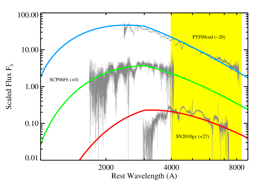
Figure 1: SLSN-I spectral templates (thick blue, green, and red lines) compared to the actual spectra of supernovae at 3 different phases (20 days before maximum, near maximum, and 27 days after maximum in the rest frame ROTSE-IIIb system). The spectra of PTF09cnd, SCP 06F6, and SN 2010gx are taken from Quimby et al. (2011), Barbary et al. (2009), and Pastorello et al. (2010), respectively. The yellow shaded area marks the ROTSE-IIIb rest frame band pass.

Near maximum light, which is the most important phase for our rate calculation, the features present in the rest frame ROTSE-IIIb are very weak in comparison to normal supernovae, so the temperature of the black body is the main concern. The results of Chomiuk et al. (2011) suggest that SLSN-I follow similar cooling curves, although there may be a range of peak temperatures. We note that the SDSS-II photometry of SN 2006oz indicates a nearly constant photospheric temperature with time (Leloudas et al. 2012), and the earliest phases are cooler than our simple model. The peak of this particular event is not well constrained, so we cannot include it in our efficiency calculations.

For the SLSNe-II, we assume a simple Planck function for the SED. This is motivated by events like SN 2008es, which was well observed and found to be well fit by a black body (Miller et al. 2009; Gezari et al. 2009), and other SLSNe-II like SN 2006tf (Smith et al. 2008a) and SN 2008am (Chatzopoulos et al. 2011), which, apart from their hydrogen emission lines, are reasonably well approximated by black bodies. The temperature measured at peak for SN 2008es ($\sim$14,000 K) is much higher than for SN 2006tf ($\sim$8000 K), but both objects cool in a similar manner as they fade. We find that the temperature evolution of SLSNe-II can be parameterized as $T(\eta)=11.8-15.3\eta+14.4\eta^{2}-4.2\eta^{3}$ (in units of $10^{3}$ K; see Fig. 2). The parameter, $\eta$, is a function of the peak absolute magnitude in the rest frame ROTSE-IIIb band, $M_{peak}$, and the decline from peak, $\Delta M$, such that $\eta=0.25(M_{peak}+22)-\Delta M$ before peak and $\eta=0.25(M_{peak}+22)+\Delta M$ after. The $\eta$ parameter thus corresponds to the drop in magnitudes below peak (with negative values for pre-maximum phases) normalized to the behavior of a $M=-22$ source. We limit $\eta$ to $-0.4<\eta<0.8$, so the temperatures can be up to 20000 K early on, but never below 6700 K at later times. We have also experimented with other ad hoc parameterizations of the temperature evolution, but these made no significant changes to our results.

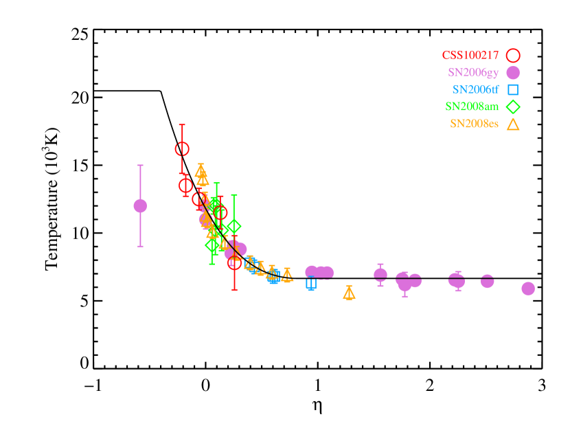
Figure 2: Blackbody temperature of SLSNe-II as a function of the parameter, $\eta$, described in the text. The symbols with error bars plot individual measurements from Drake et al. (2011), Smith et al. (2007), Smith et al. (2008a), Chatzopoulos et al. (2011), and Miller et al. (2009). The black line is the best fit cubic polynomial for $-0.4<\eta<0.8$ and a constant above and below these limits.

To construct the final light curve templates, we fit low order polynomials to the photometry (after conversion to the rest frame ROTSE-IIIb band pass as described above). In some cases, we smoothly combine fits to the rising and declining phases to better capture asymmetries in the light curves without resorting to higher order polynomials. Since the date of maximum light depends on the k-correction, and the k-corrections depend on the phase relative to maximum light (and also the peak magnitude in the case of SLSNe-II), we begin with an initial guess for the date of maximum and iterate the k-corrections and polynomial fits until they converge. The resulting templates are shown in Figure 3. Note that our light curve templates are constrained by observations taken, on average, every 3.5 rest frame days within 20 days of maximum light (without double counting the multiple bands usually obtained on the same night).

Several of the supernovae in our light curve sample have both unfiltered ROTSE-IIIb photometry and filtered observations. After k-corrections the ROTSE-IIIb measurements are about 0.1 mag fainter than the (similarly corrected) filtered photometry of SN 2006gy and SN 2008es, and the ROTSE-IIIb measurements are about 0.1 mag brighter for Dougie and SN 2010kd. The largest discrepancy seen is for SN 2006tf, for which the ROTSE-IIIb measurements are about 0.25 mag brighter than the filtered photometry available from Smith et al. (2008a) after k-corrections. The observed ROTSE-IIIb magnitudes agree with the observed R-band measurements to within 0.1 mag over the same range (out to about 100 days after maximum light), so the discrepancy in k-corrected, absolute magnitudes is probably due in part to the k-corrections themselves (as noted above, we will assume a 0.2 mag systematic error in magnitudes for the rate measurements). In the case of SN 2006tf, we choose to shift our unfiltered photometry to match the filtered measurements. This preserves the constraints on maximum light from the ROTSE-IIIb observations, which precede the filtered data by up to 1 month.

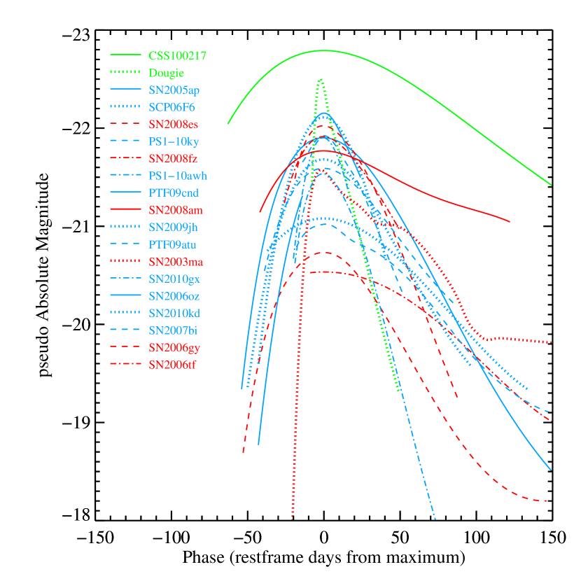
Figure 3: Light curves of SLSN-like events in the rest frame unfiltered ROTSE-IIIb band pass. Blue curves are for SLSN-I, and red curves mark SLSN-II. The green curves are for two objects of uncertain origin.

CSS100217 (Drake et al. 2011) appears to be distinctly brighter than the rest of the objects considered, and, integrating its light curve, it radiated far more energy than the others over the period shown in Figure 3. It was also located precisely coincident with a known AGN (SDSS J102912.58+404219.7; cf. Greene & Ho 2007). Drake et al. (2011) favor classifying this object as a SLSN-II because its variability is larger than normal AGN flares, but given that its amplitude is also larger than even the extreme supernovae considered here, a similar argument could be used to disfavor classification as a supernova (see further discussion in §5). Similarly, Dougie is brighter than the other remaining events, it rises and fades faster, and, as noted above, it shows a spectral evolution that is distinct from most SLSNe. While each of these may yet prove to be supernovae, the evidence against this interpretation is considerable. We will thus calculate the SLSN rates below with and without these questionable events.

3.2 SLSN Pseudo-Absolute Magnitude Distribution

From the light curve templates constructed above, we derive the approximate pseudo-absolute magnitude distribution of SLSNe-I and SLSNe-II. Ideally, one would like to have a volume limited sample from which to derive these distributions. This is simply not available, and we are further limited by the small numbers in the flux limited samples. Given these limitations, it may be tempting to simply take the peak magnitudes from the light curve sample, measure the average and standard deviation, and then assume a Gaussian distribution with these parameters (and we do consider such distributions for the rate calculations below for reference). However, this will generally be problematic since the observed sample is flux limited and thus lacking representation from the lower luminosity members of the true population. The mean and standard deviation from the observed samples will thus be biased. Additionally, real, astrophysical sources that lie in star-forming galaxies will be obscured by dust. This will skew an intrinsically Gaussian distribution and produce an extended faint tail to the pAMD.

We thus attempt to derive realistic pAMDs from the data available by assuming the intrinsic populations obey a Gaussian distribution for simplicity and including the skewing effects of dust. To translate these ideal models into the distributions recovered by a flux limited search, we simply weight the ideal distributions by the relative volumes expected from such a survey. We can then find the best pAMD (the one that would be found from an ideal, volume limited survey) by varying the input model until the best match is found between the weighted model and the observed sample. As the model separates the effects of dust from the intrinsic scatter, insights into the later may be gained if the correct dust model is used. SN 2006oz was not observed at maximum light, so we must exclude it from what follows.

The sample is based on discoveries drawn from several different surveys, each with their own selection biases. The ultimate selection function for our light curve sample is thus complex and largely unknown. To simplify matters, we assume the aggregate population is selected from a hypothetical, flux limited survey. This should be a reasonable assumption since the contributing surveys are flux limited (not targeting specific luminosity ranges or host galaxy types) at their core, with spectroscopic follow-up adding a second roughly flux limited layer to the discovery process. There could be additional biases, however, such as a preference for publication of the higher luminosity events, that may further skew our light curve sample. Such effects should typically limit the inclusion of lower-luminosity events (in particular, we note that the sample from Gal-Yam 2012 is based on events that peak above $-21$ mag in any given photometric system). This could lead us to overestimate our survey efficiency and thus underestimate the rates.

We consider simple models for the pAMDs based on intrinsic luminosity functions that follow a Gaussian distribution combined with host absorption drawn from an exponential distribution of the form $P(A_{V})\propto e^{-A_{V}/\tau}$ (the V-band is the best match to the ROTSE-IIIb band when redshifted to $z\sim 0.2$). We adopt $\tau=0.6$ for the SLSN-I and SLSN-II populations because these events are very likely to be connected with massive stars and the absorption distribution expected for objects originating from such stars is approximately fit with this exponential distribution (Hatano, Branch & Deaton 1998). As shown below, this choice also provides a reasonable match to the observed distributions of SLSN in the light curve sample after transforming the pAMD models to the distributions expected from a flux limited survey.

With $\tau$ fixed, we vary the model’s peak (intrinsic) magnitude, $M$, and its Gaussian width, $\sigma$ to find the best match to the light curve sample. We measure the maximum offsets in the cumulative distributions of the models and data and we record the Kolmogorov-Smirnov probability that the observed distribution was drawn from each model. Given the limited SLSN-I and SLSN-II sample sizes, a variety of values are plausible, but we find the best agreement for the SLSN-I sample around $M=-22.0$ and $\sigma=0.3$, while the SLSN-II population is best matched with values around $M=-21.4$ and $\sigma=0.6$. The peaks of the intrinsic distributions cannot be much brighter (e.g. $M\mathrel{\hbox{\hbox to0.0pt{\hbox{\lower 4.0pt\hbox{$\sim$}}\hss}\hbox{$>$}}}-22.3$ for the SLSN-I), but fainter values are plausible if the widths of the distributions are larger. We did not allow the absorption distribution to vary, but smaller values of $\tau$ would decrease the expected number of the lower luminosity events, which is less preferred (but not excluded). We considered observed distributions both with and without CSS100217 and Dougie, but the differences are negligible. The resulting pAMD models are shown in Figure 4.

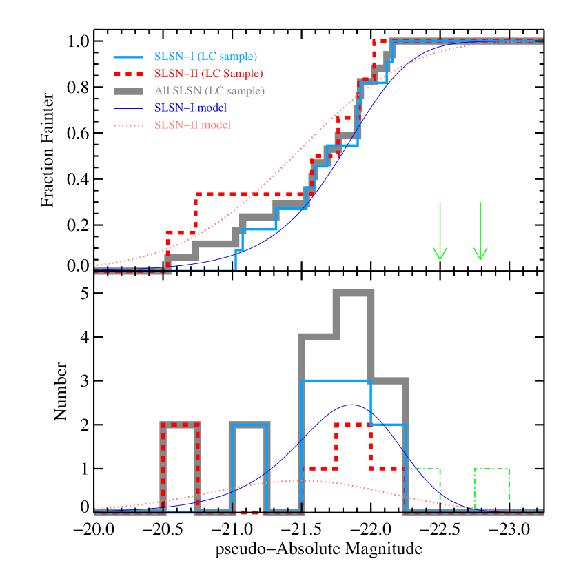
Figure 4: Peak pseudo-absolute magnitudes for SLSN-I (blue) and SLSN-II (dashed red) in the light curve sample. SN 2006oz is not included because its peak magnitude is not well constrained. The locations of CSS100217 and Dougie, which may or may not actually be SLSNe, are marked with the green arrows on the top plot (cumulative distribution) and dashed-dotted green boxes on the lower plot (binned distribution). The dark blue and dotted pink curves show the models used in the survey efficiency calculations adjusted for the selection effects of a flux limited survey for comparison to the observed sample. The SLSN-I model has an intrinsic Gaussian width of just $\sigma=0.3$ mag. The skewed faint end tail of the model is a result of the assumed host absorption distribution.

We have included SN 2007bi and SN 2010kd in the SLSN-I light curve sample even though their light curves decline (and likely rise) much more slowly than the other SLSN-I, which could point to a different physical origin (Gal-Yam et al. 2009 have concluded that SN 2007bi is a radioactively powered, pair-creation supernova, but this possibility is excluded for others in the SLSN-I sample). Even with these events, the width of the intrinsic luminosity function could be rather narrow. If there is a publication bias against lower luminosity SLSN-I, then the true distribution could be broader than the available evidence suggests. It is also possible to explain the observed scatter in SLSN-I peak magnitudes from the effects of dust alone, with zero intrinsic dispersion (assuming the dust model adopted above).

We estimate the uncertainty in the peaks of our distributions by varying the temperatures assumed in calculating the k-corrections for our light curve sample. To determine the systematic error, we adjust the model temperatures by $\pm 1000$ K, and add to this an estimate of the statistical uncertainty in the peak magnitudes.

4 The SLSN Rates

In this section, we combine the ROTSE-IIIb sample presented in section 2 and the light curves and pAMDs infered from the published sample of SLSNe (presented in section 3) to derive the volumetric rates of SLSN-I, SLSN-II, and all SLSN-like objects (which may include additional, rare phenomena that may or may not be true supernovae). The rates are calculated from,

$$R={N\over\sum_{i}\epsilon_{i}V_{i}t_{i}}$$ (1)

with $N$ the number of events detected, $V_{i}$ the co-moving volume element for the $i^{\rm th}$ distance bin, $\epsilon_{i}$ the corresponding survey efficiency for that bin, and $t_{i}$ the proper time for the survey in each bin. We refer to the denominator in eqn. 1 as the “effective volume-time” in what follows. We first describe the Monte Carlo simulations employed to calculate the survey efficiency before presenting the actual rates.

4.1 Monte Carlo Simulations

Following the procedure described in Quimby et al. (2012), we have run Monte Carlo simulations to determine how efficient our ROTSE-IIIb search has been in selecting SLSNe. We define our survey efficiency, $\epsilon_{i}$, as the fraction of SLSNe in a given volume that we are likely to select. There are two main factors in selecting SLSNe: 1) are the observations deep enough to detect a given SLSNe at a given distance, and 2) did we observe the appropriate sky location during the right time to catch the transient during outburst (relevant only if the observations are deep enough). The first factor results from the flux limited (i.e. not volume limited) nature of our survey. At a given distance we may detect some of the more luminous SLSNe but miss some of the fainter events. The second factor is a result of our sampling function (or “cadence”). Due to weather, observing seasons, and time constraints, we have not observed the same fields every day, and some fields have far less coverage that others (see figures 1 and 2 from Quimby et al. 2012), so we could have missed even bright SLSNe in coverage gaps. We thus perform a Monte Carlo simulation in which we compare SLSNe light curves at various sky locations, distances, and random explosion dates to the actual survey data to determine what fraction of simulated events we are likely to have selected.

We determine our selection efficiency in distance bins from 40 to 4000 Mpc (beyond this our selection probability is zero, as we will show below). For each distance bin, we convert the absolute magnitude light curves from section 3 to their expected (or “observed”) magnitudes by adding the distance modulus, the same crude k-corrections described above, and the Galactic extinction from Schlegel, Finkbeiner & Davis (1998) for a given sky position. Next we randomly select a date for maximum light between Nov 1, 2004 and January 31, 2009. The observed magnitude can then be computed for any day over the survey period. We compare the expected magnitudes for our simulated SLSNe to the actual data recorded to determine the fraction of events likely to have been selected. To do this, we use the detection efficiency curves from Quimby et al. (2012), which give the probability of detecting an object as a function of magnitude. These detection efficiency curves take into account the seeing quality for the image as well as the “limiting magnitude.”

In the actual survey, the selection of targets was done by humans reviewing an automatically generated “short list” of candidates that was constructed from targets with at least a $5\sigma$ detection in a nightly image stack, and at least $2.5\sigma$ detections in the first and second halves of the night (in addition to other cuts on shape parameters and increase in brightness; see Quimby et al. 2012 for full details). Thus, in our simulations we calculate the detection probabilities on each of the three stacks, draw three random numbers (uniformly distributed between 0 and 1), and we only count a simulated source as recovered if each of the three probabilities is larger than their respective random draws.

As in Quimby et al. (2012), we compare the expected distributions in the distance, observed peak magnitudes, pseudo absolute magnitudes, and the number of nights a simulated source is detected from the simulations to the observed data. Given our small sample size, we lack the statistical power to identify differences between how the simulated sources are selected versus the actual survey data; however, we do note that not one event in our observed sample was detected on fewer than 5 nights. In contrast, the simulations typically predict that $\sim$60% of our discoveries should only be detectable on 4 or fewer nights. Quimby et al. (2012) found a similar disagreement between the models and data for a larger sample of Type Ia supernovae, which could be resolved by considering only the events (real or simulated) detected on 5 or more nights. The dearth of objects detected on just 1-4 nights is presumably attributed to human bias in the selection of targets. We assume a similar effect for our SLSN sample and limit the models and data to events detected on 5 or more nights. With this cut, the four model distributions considered appear to be well matched with the observations. If we were to ignore this selection cut, the rates found below would be lowered by a factor of 2.5.

4.2 SLSN-I Rates

We have only one discovery, SN 2005ap, from which to derive the SLSN-I rate. Obviously, our rate will be subject to the eccentric properties of small number statistics, and care should be taken in interpreting these results.

We first perform Monte Carlo simulations using the SLSN-I light curves from section 3 (excluding Dougie for the moment) and the the SLSN-I pAMD model derived in section 3.2 to determine our effective volume-time. Under these assumptions, the effective volume-time of the ROTSE-IIIb search is $0.0315$ Gpc³ yr¹ $h_{71}^{-3}$, which gives a rate of $(32^{+77}_{-26})$ events Gpc^-3 yr^-1 $h_{71}^{3}$, where the error bars account for only the statistical Poisson fluctuations (Gehrels 1986).

To estimate our systematic error, we recalculate our survey efficiencies with the input pAMDs shifted 0.2 mag brighter or fainter. This is to account for possible systematic error in our k-corrections, which may bias the peak magnitude distributions. Given our small sample size, the statistical errors dominate the systematics, which we find to be ${}^{+10}_{-7}$ events Gpc^-3 yr^-1 $h_{71}^{3}$ for the SLSN-I. We note, however, that due to selection (and particularly publication) bias, our pAMD may not accurately represent the full population of events physically connected to the SLSNe-I. In this case, our rates are valid only for the luminosity range considered and are simply lower limits for the greater population.

Figure 5 shows our survey efficiency as a function of luminosity distance. The expected distance distribution of SLSN-I is also shown with the solid blue curve. This latter curve is calculated by multiplying the efficiency curve by the relative volume and proper time in each distance bin. Although the sensitivity curve drops off above $\sim$300 Mpc, this is initially compensated for by the nearly cubic rise in volume with distance. Due to this rise in volume, we are sensitive to SLSN-I out to more than 2000 Mpc even though we may detect less than 1% of this population. We expect to find about 97% of our SLSN-I between 200 and 2000 Mpc (roughly $0.05<z<0.4$), and half should be farther than about 800 Mpc. Note that at $D_{L}\sim 1440$ Mpc, SN 2005ap falls comfortably with in our expectations. The average effective redshift for our SLSN-I rate measurement is thus $z=0.17$.

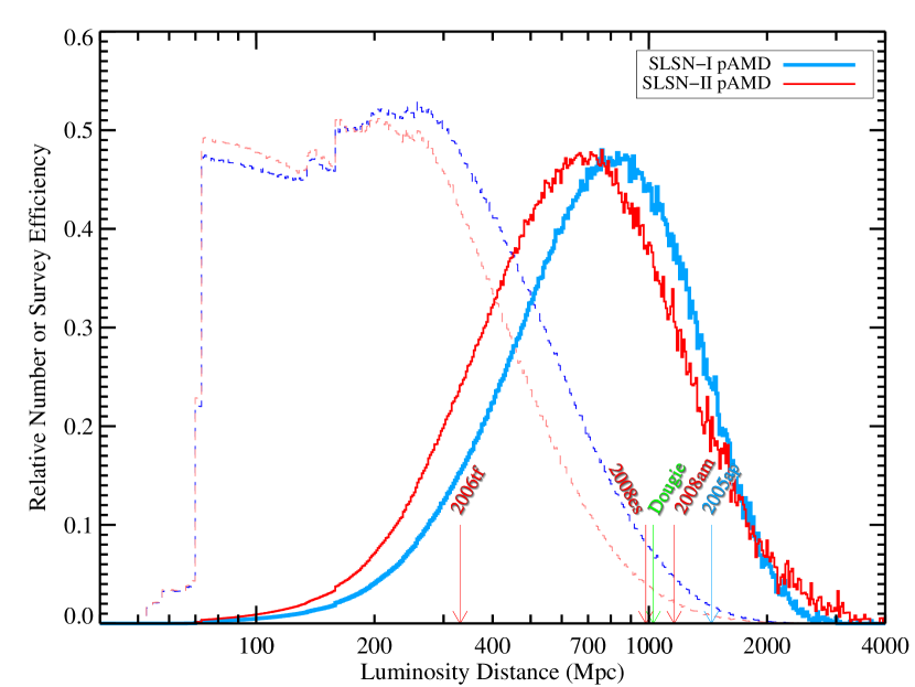
Figure 5: Survey efficiencies (dashed lines) and the relative distance distributions (solid lines) of SLSN-I (blue curves) and SLSN-II (red curves) expected from these. The luminosity distances for the SLSNe in the ROTSE-IIIb sample are indicated with arrows.

As a check, we also provide effective volume-times assuming only the light curves of individual supernovae and two separate assumptions on the peak magnitude distribution in table 2. The values in the fifth column assume that the distribution is a simple Gaussian (no skewing by host absorption) that takes the reported peak magnitude of the supernova for the peak of the distribution and assumes a width of $\sigma=0.3$ mag. This width was chosen to represent the (assumed) intrinsic scatter in events otherwise identical to each object listed and is based on the intrinsic scatter of SLSN-I estimated above. For SN 2005ap, the effective volume-time is $0.0504$ Gpc³ yr¹ $h_{71}^{-3}$ under these assumptions. From equation 1, this leads to a rate of $(20^{+48}_{-16})$ events Gpc^-3 yr^-1 $h_{71}^{3}$ (statistical error only).

The sixth column in table 2 gives the effective volume-times again assuming only the single light curve of the supernova and a simple, uncorrected Gaussian distribution but with the peak and width set by the average and standard deviation of the apparent SLSN-I sample, respectively ($M=-21.7$ and $\sigma=0.4$ mag). With these assumptions, the effective volume-time drops to $0.0288$ Gpc³ yr¹ $h_{71}^{-3}$. The rate for this distribution is then $(35^{+84}_{-29})$ events Gpc^-3 yr^-1 $h_{71}^{3}$.

Our original measurement is fully consistent with these two later assessments. Again, the small sample size (one object) results in large statistical errors which dominate systematic concerns. As the procedure used to estimate the pAMD model is generally less prone to bias than the later, simple Gaussian assumptions, we retain its effective volume-time for our best measurement of the SLSN-I rate.

If we count Dougie as a SLSN-I, then the effective volume-time (including Dougie and all SLSN-I light curves in the Monte Carlo simulations) decreases slightly to 0.0291 Gpc³ yr¹ $h_{71}^{-3}$. The combined rate for these two events is then $(68^{+94}_{-44})$ events Gpc^-3 yr^-1 $h_{71}^{3}$ (statistical error only).

4.3 SLSN-II Rates

Our ROTSE-IIIb sample includes three events with clear signatures of hydrogen in their spectra: SNe 2006tf, 2008am, and 2008es. Although they share some similar properties, there are differences as well. In particular, the available observations of SN 2008es do not show the obvious narrow emission lines from hydrogen. These are present in the spectra of SNe 2006tf and 2008am and suggest an interaction of the supernova ejecta with slow moving circum-stellar material as a contributing power source. It could be, however, that SN 2008es experienced a similar interaction prior to the first available spectra (cf. Moriya & Tominaga 2012).

Given the apparent differences, one could follow a similar procedure as outlined above and calculate three separate rates using the effective volume-times in Table 2. Here we use the full ensemble of SLSN-II light curves available in the light curve sample and the pAMD model from section 3.2 to place limits on the bulk, hydrogen rich SLSN population.

Using the SLSN-II pAMD model, we find an effective volume-time of $0.0199$ Gpc³ yr¹ $h_{71}^{-3}$ (this would be 6% larger if the light curve of CSS100217 were included). From equation 1, this gives a SLSN-II rate of $(151^{+151}_{-82})$ events Gpc^-3 yr^-1 $h_{71}^{3}$ (statistical error only) for our sample of three events. Performing the same check described above, we estimate a systematic error of ${}^{+52}_{-33}$ events Gpc^-3 yr^-1 $h_{71}^{3}$. Again, we stress that there could be lower luminosity events that are physically related to those considered in determining the pAMD. In this case, our rate is a lower limit on the greater population.

From Figure 5, it is apparent that like the SLSN-I, we are sensitive to SLSN-II in roughly the 200 to 2000 Mpc range. The average redshift for our SLSN-II rate measurement is $z=0.15$.

4.4 SLSN-Like Rates

Finally, we measure the total rate of SLSN-like events including possible tidal disruption events or rare, supernova-like outbursts from (uncatalogued) AGN. Our survey was not intentionally biased against events located near galaxy nuclei (for example, SN 2006gy was found less than 0.3 pixels from the core if its host), but we did exclude a few sources detected coincident with known AGN. Our detection efficiency was also calculated for blank sky locations only, so it may be an overestimation for sources on top of bright galactic nuclei. So once again, our rate may be considered a lower limit.

We include Dougie with the other 4 background events and assume the effective volume-time is simply given by the average of the SLSN-I and SLSN-II values found above (including Dougie and CSS100217 in the Monte Carlo simulations). Since the pAMDs for these two groups are broadly similar, this should be a reasonable approximation. With these assumptions, the total SLSN-like rate is $(199^{+137,+65}_{-86,-41})$ events Gpc^-3 yr^-1 $h_{71}^{3}$, where the first and second errors quoted are statistical and systematic, respectively.

5 Conclusions and Discussion

We have produced a set of SLSN light curve templates corrected to the rest frame, unfiltered ROTSE-IIIb band pass and used these to estimate the pseudo-absolute magnitude distributions of SLSN-I and SLSN-II. With these and our sample of ROTSE-IIIb discovered SLSN (and a SLSN-like event), we have calculated the volumetric rates in the local volume ($\overline{z}\sim 0.2$). Compared to the $z\sim 0.2$ core collapse supernova (CCSN) rate (cf. Botticella et al. 2008)), we find that there is about one SLSN-I or SLSN-II event for every 400 to 1300 CCSNe, or one SLSN-I for every $1000$ to $2\times 10^{4}$ CCSNe (these fractions may be halved if the full population of faint or obscured CCSNe is included; Horiuchi et al. 2011). The total SLSN-like rate is also similar to the local rate of sub-energetic, long-duration gamma-ray bursts (LGRB; Soderberg et al. 2006), although the SLSN-like and LGRB samples are currently too small for a definitive comparison.

If the SLSNe rates simply track the cosmic star formation rate (CSFR), then, using the parameterization of Yüksel et al. (2008), the CSFR and thus SLSN rate should be about 5 times larger at $z\sim 3$ than we have measured for the nearby ROTSE-IIIb sample. Given the large errors, this could be roughly consistent with the rate of SLSNe at $z\sim 2$ and 4 (Cooke et al. 2012). However, the search performed by Cooke et al. (2012) was likely biased to longer duration events, and they suggest their discoveries represent only the radioactively powered subset of SLSNe (and only a fraction of those). In this case, their high redshift discoveries could imply an enhancement over a simple scaling by the CSFR when compared to an appropriate fraction of our low redshift rates, as they have noted.

The SLSN-I in the light curve sample are particularly interesting. Although these events were observed in a variety of (rest frame) band passes and we apply only a simplistic k-correction, they still appear to constitute a surprisingly uniform class when transformed to the ROTSE-IIIb system (see Fig. 3). The light curves show some quantitative differences but tend to rise smoothly over around 50 rest frame days, which is considerably longer than typical Type Ia supernovae. Several SLSN-I also show smooth declines that almost mirror their pre-maximum behavior. The peak magnitudes of the SLSN-I in the light curve sample have an average of $-21.7$ mag and a standard deviation of $\pm 0.4$ mag. Our best estimate of the intrinsic scatter (after accounting for absorption in the host galaxies and selection bias) is about $\pm 0.3$ mag, but this is not well constrained. These values are based on a small sample (10 events) and change negligibly if Dougie is added. Given that the peak magnitudes of the SLSN-I sample are relatively tightly distributed, it is worth considering if this is a mere selection bias or indicative of a population that may prove useful as standard candles.

First, we consider the high luminosity cutoff to the distribution. The published sample of SLSN-I shows a cap in peak absolute magnitudes close to $M\sim-22$. If there are such events with significantly brighter peaks they must be exceedingly rare or they would dominate flux limited searches. It is thus reasonable to conclude that most SLSN-I will peak around $-22$ mag or fainter.

Next, we consider the lower luminosity limit for the SLSN-I available in the light curve sample. Formally, we have used an arbitrary cut on peak luminosities ($M_{\rm peak}<-21$) to select the SLSN-I for our light curve sample, but we note that we could use other, luminosity independent criteria to define this sample. In particular, the SLSN-I in the light curve sample contain the only supernovae we know of that show OII features in their maximum light spectra. Other supernovae with more normal peak luminosities may also display such features at very early times, but these quickly disappear as the ejecta cool and oxygen recombines (cf. the spectral series of SN 2008D presented by Modjaz et al. 2009). As a practical matter, this definition is perhaps less useful than a simple luminosity cut as it requires reasonably high signal to noise spectra taken at the right phase and with the proper wavelength coverage to catch the relatively weak OII features in the 4400 to 5800 Å range. Indeed, The wavelength coverage and signal to noise of SCP 06F6 and PS1-10ky preclude a definitive assessment of such features at maximum light, but based on the available spectral information (particularly the high temperatures implied and the similar features at 2100 to 2700 Å), we find this to be likely. There are no spectra of SN 2007bi near maximum light, but we suspect the OII features would have been visible at maximum as well considering later phase spectroscopic matches to the SLSN-I sample.

There are no known supernovae of normal luminosities that show OII at maximum light (events with this feature at maximum will be called SN 2005ap-like hereafter), and this signature may uniquely identify a potentially useful population of high luminosity supernovae. Based on the considerations below, we find it likely that all SN 2005ap-like events will be superluminous because the OII lines require high temperatures and the long expansion of the ejecta up to maximum light necessitate a large radius. The maximum light spectra of SLSN-I are reasonably well approximated by a black body (at least in the optical range where line blanketing is not an issue; Pastorello et al. 2010, Chomiuk et al. 2011; see Fig. 1), so the peak luminosity of SLSNe-I will be approximately, $L=4\pi R^{2}\sigma T^{4}$ (with a small dilution term to correct for the departure from a black body, which we neglect). Hatano et al. (1999) have shown that OII features are temperature sensitive. These lines should be replaced by the usual OI lines for temperatures below about 12000 K, and by OIII lines for temperatures above 15000 K. The typical expansion velocity of supernovae, $10^{4}$ km s^-1 over a one month period gives a radius of $\sim 3\times 10^{15}$ cm. Thus any supernova that remains hot enough to display prominent OII features after a one month rise to maximum light should have a peak absolute magnitude brighter than about $M=-21$.

More detailed theoretical modeling, beyond the scope of this paper, is required to verify this simplified picture and determine if all SN 2005ap-like supernovae must necessarily reach such high luminosities. If the observed floor to the peak magnitude distribution proves to be physical and not just a selection effect, then the peak magnitudes of SN 2005ap-like supernovae are confined to a relatively narrow range. This gives potential for SN 2005ap-like supernovae to one day serve as standard candles visible as far as $L_{*}$ galaxies can be seen and clearly warrants further study.

We next consider if SLSN-I obey a luminosity-decline relation analogous to the Phillips relation observed for the standard bearer of standard candles, Type Ia supernovae. In Figure 6, we plot the change in magnitude between peak and 40 days after peak, $\Delta m_{40}$, against peak pseudo-absolute magnitude. SLSNe may be better differentiated in their declines from peak at even later phases, but the observations are harder to come by. Errors shown are the estimated statistical error plus an estimate of the systematic error based on changing the temperature of the SED used in the k-correction, as discussed above.

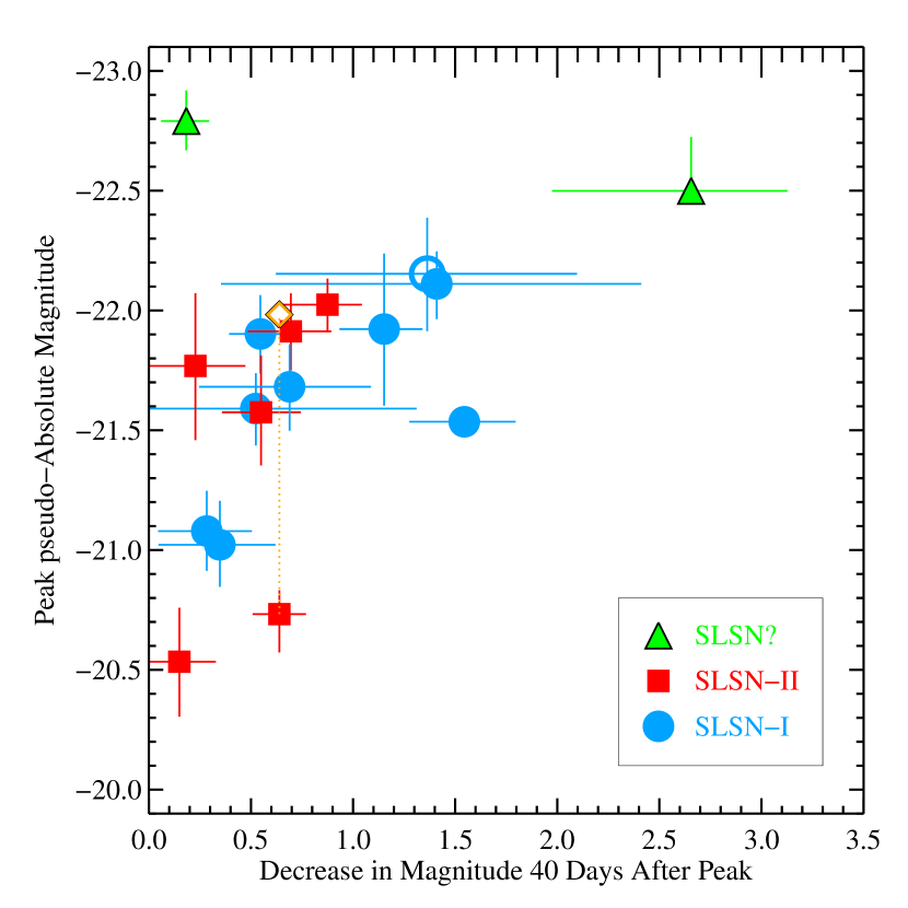
Figure 6: Photometric decline in magnitudes between peak and 40 days after peak for the SLSN light curve sample. The open orange diamond shows where SN 2006gy would lie if corrected for host absorption. The open circle marks SN 2005ap, which was not observed on day $+40$ or after; the $\Delta m_{40}$ shown for SN 2005ap is an extrapolation of the earlier light curve. Errors include the estimated systematics.

Using the Bayesian linear regression routine, linmix_err.pro (Kelly 2007), we do not find a significant correlation for 9 SLSN-I plotted in Figure 6. If we include Dougie, however, there may be a weak correlation between the peak magnitudes and decline parameter in the sense that brighter events have faster declines. This may simply be a selection effect, however, which would tend to remove the fainter, faster declining events.

Figure 6 also includes the SLSN-II from the light curve sample. It is interesting to note that if the peak magnitude of SN 2006gy is corrected for host absorption, then the combined distribution of SLSN-I and SLSN-II peaks sharply at $M\sim-21.8$ with SN 2006tf the only SLSN-II falling below. It is unclear if this event is the low luminosity tail of the SLSNe-II population or the bright tail of the “normal” Type IIn supernova distribution. Indeed, it is unclear if two such distinct populations exist in nature, or if there is simply a publication bias against Type IIn supernovae of moderately bright luminosities. Any such distinction may be borne out by the larger samples of normal supernovae and SLSNe currently being gathered by searches such as PTF, Pan-STARRS, the Catalina Real-Time Transient Survey (Drake et al. 2009), and La Silla-QUEST (Hadjiyska et al. 2012).

The discovery of such rare events, however, may be hindered by contamination from other transient phenomena. The ROTSE-IIIb sample includes about ten times more SNe Ia than SLSNe-like events even though the SLSNe are observable over a much larger volume because the ratio of the rates is even larger. There is also the worry that other rare transient phenomena, such as tidal disruption flares or an outburst from an AGN with a supernova-like light curve, could contaminate the sample. We potentially have one such source in our ROTSE-IIIb sample: Dougie. If Dougie proves to be a hydrogen poor supernova, our SLSN-I rate would roughly double.

The SLSN-II population may similarly be polluted with AGN activity. Drake et al. (2011) favor classifying CSS100217 as a superluminous supernova even though it radiated far more light than other SLSN published so far. CSS100217 does show features present in Type IIn supernova, but these are not unique to supernovae and can also mark an AGN outburst (see Colgate & Cameron 1963 and Filippenko 1989 for a discussion of the similarities between AGN and SNe IIn spectra). Since the host of CSS100217 is known to harbor an AGN and this is precisely coincident with the transient, this could simply be a demonstration of rare AGN related activity. Drake et al. (2011) note that amplitude of CSS100217’s outburst stands distinct from typical AGN, but CSS100217 was specifically selected for this unusual brightening while the comparison sample was drawn from the SDSS DR3 spectroscopic sample (i.e. not selected based on variability). The relatively large effective volume-time for CSS100217-like events listed in Table 2 indicates that such events are either very rare (least they dominate flux limited surveys, which is not the case), or they must be selected against due to, for example, the presence of a coincident AGN. We know of no reason to exclude AGN from having supernova-like outbursts, so it will be important to measure the rate of such events to determine their potential contamination to supernovae samples.

Like CSS100217, SN 2006gy was located near the core of its host (but clearly offset in this case). Studies of our own galaxy and M31 have uncovered a significant population of massive stars located very close to the central nuclei (Genzel et al. 2000; Lauer et al. 2012). We speculate that such environments may on occasion harbor dense clouds of gas accreted from the disk (cf. Levin & Beloborodov 2003), recent galaxy mergers, or fed by filaments, and these special environments may yet give birth to unusual supernovae. These events may be heavily extincted and thus difficult to detect (e.g. SN 2006gy suffers from about 1.25 mag of absorption in the R-band). This may add to the confusion with AGN and make the SLSN-II rate difficult to measure.

The rates presented here may be helpful in determining the origin of SLSNe. For example, using the total star formation rate at z=0.16 (Hopkins & Beacom 2006) and a modified Salpeter IMF (Baldry & Glazebrook 2003), we can compare our total SLSN rate to the expected production rate of stars with $56M_{\sun}\mathrel{\hbox{\hbox to0.0pt{\hbox{\lower 4.0pt\hbox{$\sim$}}\hss}\hbox{$<$}}}M_{\rm initial}\mathrel{\hbox{\hbox to0.0pt{\hbox{\lower 4.0pt\hbox{$\sim$}}\hss}\hbox{$<$}}}84M_{\sun}$, which is the mass range under which zero metallicity stars are expected to enter the pulsational pair instability regime (Chatzopoulos & Wheeler 2012; Yoon, Dierks & Langer 2012). We find that our SLSN rate could be explained by a small fraction of the stars born in this mass range (about 1 to 3% at the $1\sigma$ confidence level). To put this another way, we can say at the $>10\sigma$ confidence level that at $z\sim 0.2$, not all stars in this mass range produce supernovae brighter than $M\sim-21$ mag; if some of these stars do produce SLSNe, others must experience alternate fates. These rates also define a basis for comparison to future, higher redshift studies, which may help determine if the IMF varies over the distances that will be probed by forthcoming surveys (i.e. $z\sim 4$ with Subaru Hyper-SuprimeCam).

References

- Akerlof et al. (2003) Akerlof C. W. et al., 2003, PASP, 115, 132
- Baldry & Glazebrook (2003) Baldry I. K., Glazebrook K., 2003, ApJ, 593, 258
- Barbary et al. (2009) Barbary K. et al., 2009, ApJ, 690, 1358
- Berger et al. (2012) Berger E. et al., 2012, ApJ, 755, L29
- Botticella et al. (2008) Botticella M. T. et al., 2008, A&A, 479, 49
- Chatzopoulos & Wheeler (2012) Chatzopoulos E., Wheeler J. C., 2012, ApJ, 748, 42
- Chatzopoulos et al. (2011) Chatzopoulos E. et al., 2011, ApJ, 729, 143
- Chevalier & Irwin (2011) Chevalier R. A., Irwin C. M., 2011, ApJ, 729, L6
- Chomiuk et al. (2011) Chomiuk L. et al., 2011, ApJ, 743, 114
- Colgate & Cameron (1963) Colgate S. A., Cameron A. G. W., 1963, Nature, 200, 870
- Cooke et al. (2012) Cooke J. et al., 2012, Nature, 491, 228
- Dahlen et al. (2012) Dahlen T., Strolger L.-G., Riess A. G., Mattila S., Kankare E., Mobasher B., 2012, ApJ, 757, 70
- Dessart et al. (2012) Dessart L., Hillier D. J., Waldman R., Livne E., Blondin S., 2012, ArXiv e-prints
- Drake et al. (2011) Drake A. J. et al., 2011, ApJ, 735, 106
- Drake et al. (2009) —, 2009, ApJ, 696, 870
- Drake et al. (2010) —, 2010, ApJ, 718, L127
- Filippenko (1989) Filippenko A. V., 1989, AJ, 97, 726
- Filippenko et al. (2001) Filippenko A. V., Li W. D., Treffers R. R., Modjaz M., 2001, in Astronomical Society of the Pacific Conference Series, Vol. 246, IAU Colloq. 183: Small Telescope Astronomy on Global Scales, Paczynski B., Chen W.-P., Lemme C., eds., p. 121
- Foley et al. (2006) Foley R. J., Li W., Moore M., Wong D. S., Pooley D., Filippenko A. V., 2006, Central Bureau Electronic Telegrams, 695, 1
- Gal-Yam (2012) Gal-Yam A., 2012, ArXiv e-prints
- Gal-Yam et al. (2009) Gal-Yam A. et al., 2009, Nature, 462, 624
- Gehrels (1986) Gehrels N., 1986, ApJ, 303, 336
- Genzel et al. (2000) Genzel R., Pichon C., Eckart A., Gerhard O. E., Ott T., 2000, MNRAS, 317, 348
- Gezari et al. (2009) Gezari S. et al., 2009, ApJ, 690, 1313
- Graur et al. (2011) Graur O. et al., 2011, MNRAS, 417, 916
- Greene & Ho (2007) Greene J. E., Ho L. C., 2007, ApJ, 667, 131
- Hadjiyska et al. (2012) Hadjiyska E. et al., 2012, in IAU Symposium, Vol. 285, IAU Symposium, Griffin E., Hanisch R., Seaman R., eds., pp. 324–326
- Harutyunyan et al. (2006) Harutyunyan A., Benetti S., Turatto M., Cappellaro E., Elias-Rosa N., Andreuzzi G., 2006, Central Bureau Electronic Telegrams, 647, 1
- Hatano, Branch & Deaton (1998) Hatano K., Branch D., Deaton J., 1998, ApJ, 502, 177
- Hatano et al. (1999) Hatano K., Branch D., Fisher A., Millard J., Baron E., 1999, ApJS, 121, 233
- Hopkins & Beacom (2006) Hopkins A. M., Beacom J. F., 2006, ApJ, 651, 142
- Horiuchi et al. (2011) Horiuchi S., Beacom J. F., Kochanek C. S., Prieto J. L., Stanek K. Z., Thompson T. A., 2011, ApJ, 738, 154
- Kaiser et al. (2010) Kaiser N. et al., 2010, in Society of Photo-Optical Instrumentation Engineers (SPIE) Conference Series, Vol. 7733, Society of Photo-Optical Instrumentation Engineers (SPIE) Conference Series
- Kasen & Bildsten (2010) Kasen D., Bildsten L., 2010, ApJ, 717, 245
- Kelly (2007) Kelly B. C., 2007, ApJ, 665, 1489
- Knop et al. (1999) Knop R. et al., 1999, IAU Circ., 7128, 1
- Lauer et al. (2012) Lauer T. R., Bender R., Kormendy J., Rosenfield P., Green R. F., 2012, ApJ, 745, 121
- Law et al. (2009) Law N. M. et al., 2009, PASP, 121, 1395
- Leloudas et al. (2012) Leloudas G. et al., 2012, A&A, 541, A129
- Levin & Beloborodov (2003) Levin Y., Beloborodov A. M., 2003, ApJ, 590, L33
- Li et al. (2011) Li W. et al., 2011, MNRAS, 412, 1441
- Miller et al. (2009) Miller A. A. et al., 2009, ApJ, 690, 1303
- Modjaz et al. (2009) Modjaz M. et al., 2009, ApJ, 702, 226
- Moriya & Tominaga (2012) Moriya T. J., Tominaga N., 2012, ApJ, 747, 118
- Neill et al. (2011) Neill J. D. et al., 2011, ApJ, 727, 15
- Ofek et al. (2007) Ofek E. O. et al., 2007, ApJ, 659, L13
- Ouyed et al. (2012) Ouyed R., Kostka M., Koning N., Leahy D. A., Steffen W., 2012, MNRAS, 423, 1652
- Pastorello et al. (2010) Pastorello A. et al., 2010, ApJ, 724, L16
- Prieto et al. (2006) Prieto J. L., Garnavich P., Chronister A., Connick P., 2006, Central Bureau Electronic Telegrams, 648, 1
- Quimby (2006) Quimby R. M., 2006, PhD thesis, The University of Texas at Austin
- Quimby (2008) —, 2008, in Astronomical Society of the Pacific Conference Series, Vol. 393, New Horizons in Astronomy, Frebel A., Maund J. R., Shen J., Siegel M. H., eds., p. 141
- Quimby et al. (2007) Quimby R. M., Aldering G., Wheeler J. C., Höflich P., Akerlof C. W., Rykoff E. S., 2007, ApJ, 668, L99
- Quimby et al. (2011) Quimby R. M. et al., 2011, Nature, 474, 487
- Quimby et al. (2012) Quimby R. M., Yuan F., Akerlof C., Wheeler J. C., Warren M. S., 2012, ArXiv e-prints
- Rau et al. (2009) Rau A. et al., 2009, PASP, 121, 1334
- Rest et al. (2011) Rest A. et al., 2011, ApJ, 729, 88
- Scalzo et al. (2010) Scalzo R. A. et al., 2010, ApJ, 713, 1073
- Schlegel, Finkbeiner & Davis (1998) Schlegel D. J., Finkbeiner D. P., Davis M., 1998, ApJ, 500, 525
- Smith et al. (2008a) Smith N., Chornock R., Li W., Ganeshalingam M., Silverman J. M., Foley R. J., Filippenko A. V., Barth A. J., 2008a, ApJ, 686, 467
- Smith et al. (2008b) Smith N. et al., 2008b, ApJ, 686, 485
- Smith et al. (2007) —, 2007, ApJ, 666, 1116
- Smith & McCray (2007) Smith N., McCray R., 2007, ApJ, 671, L17
- Soderberg et al. (2006) Soderberg A. M. et al., 2006, Nature, 442, 1014
- Tanaka et al. (2012) Tanaka M., Moriya T. J., Yoshida N., Nomoto K., 2012, MNRAS, 422, 2675
- Vinko et al. (2010) Vinko J. et al., 2010, Central Bureau Electronic Telegrams, 2556, 1
- Woosley (2010) Woosley S. E., 2010, ApJ, 719, L204
- Yoon, Dierks & Langer (2012) Yoon S.-C., Dierks A., Langer N., 2012, A&A, 542, A113
- Yuan (2010) Yuan F., 2010, PhD thesis, University of Michigan
- Yuan et al. (2010) Yuan F. et al., 2010, ApJ, 715, 1338
- Yüksel et al. (2008) Yüksel H., Kistler M. D., Beacom J. F., Hopkins A. M., 2008, ApJ, 683, L5
- Zwicky (1938) Zwicky F., 1938, ApJ, 88, 529