Monitoring Atmospheric Dust Spring Activity at High Southern Latitudes on Mars using OMEGA
Abstract
This article presents a monitoring of the atmospheric dust in the south polar region during spring of martian year 27. Our goal is to contribute to identifying the regions where the dust concentration in the atmosphere shows specific temporal patterns, for instance high, variable, and on the rise due to lifting or transport mechanisms. This identification is performed in relation with the seasonal ice regression. Based on a phenomenological examination of the previous results, hypothesis regarding the origin of aerosol activity of the southern polar region are proposed. This is of paramount importance since local dust storms generated in this region sometimes grow to global proportions. The imaging spectrometer OMEGA on board Mars Express has acquired the most comprehensive set of observations to date in the near-infrared (0.93-5.1 microns) of the southern high latitudes of Mars from mid-winter solstice (Ls=110°, December 2004) to the end of the recession at Ls=320° (November 2005). We use two complementary methods in order to retrieve the optical depth of the atmospheric dust at a reference wavelength of one micron. The methods are independently operated for pixels showing mineral surfaces on the one hand and the seasonal cap on the other hand. They are applied on a time series of OMEGA images acquired between LS=220° and LS=280° . As a result the aerosol optical depth (AOD) is mapped and binned at a spatial resolution of 1.0°.pixel and with a mean period of AOD sampling ranging from less than two sols for latitudes higher than 80°S to approximately six sols at latitudes in the interval 65-75°S. We then generate and interpret time series of orthographic mosaics depicting the spatio-temporal distribution of the seasonal mean values, the variance and the local time dependence of the AOD. In particular we suspect that two mechanisms play a major role for lifting and transporting efficiently mineral particles and create dust events or storms: (i) nighttime katabatic winds at locations where a favourable combination of frozen terrains and topography exists (ii) large scale ( 10-100 km) daytime thermal circulations at the edge of the cap when the defrosting area is sufficiently narrow. As regards to the source regions around the cap, the sector with the highest AOD values/variability/increase spans longitudes 180-300°E around LS 250°. Later (LS 267°) the cryptic sector becomes the most productive while the longitude sector 300-60°E remain moderately dust-generative. Our work calls for new simulations of the martian surface-atmosphere dynamics at mesoscales to reproduce the observations and confirm the interpretations.
keywords:
Mars; South Pole; Atmosphere; Dust; OMEGA.Introduction
The southern high latitudes of Mars are of great interest in spring and summer because of their role in the dust cycle. Local dust storms generated in this region sometimes develop to global storms, and a prominent dust collar encircles the polar cap. Several experiments aboard orbiters have recently contributed to elaborate and refine this picture.
The TES and MOC instruments of Mars Global Surveyor have provided a regular, but Sun-synchronous, record of dust activity in the south polar region.
Toigo et al. (2002); Imamura and Ito (2011) produced global maps of dust distribution by integrating TES individual 9 µm optical depth measurements averaged over a 5°-Ls period (respectively 10°-Ls) and binned in 5x5° boxes (respectively 5x10°, latitude, longitude). Both sets of maps depict very distinct space and time patterns of activity around the polar cap edge for the first common Martian Year (MY) 24. These seasonal trends are sometimes in contradiction. For the following Martian year 25 and 26, Imamura and Ito (2011) reported a great stability of the dust opacity disturbance compared to MY 24. Thermal mapping of dust by TES was originally limited to regions where the temperature and thus the emitted signal are sufficiently high, thus precluding the monitoring of the seasonal polar cap itself. Nevertheless Horne and Smith (2009) modified the standard TES aerosol retrieval algorithm to retrieve atmospheric dust and ice optical depth values for each daytime spectrum in the TES database with a surface temperature below 210 K. As a result maps of the seasonal and spatial variation of dust and water ice optical depth activity over both poles are presented, averaged over a 2°-Ls period and binned in 2x2° boxes from late MY24 to early MY27. For the southern high latitudes the greatest observed dust activity each year takes place above the growing seasonal cap from late summer to the beginning of winter. At other seasons dust opacity is in general much lower but some interannual variability, e.g. the beginnings of MY 25 global storm, blurs this pattern.
Following the early work of James et al. (2001) that already noted correlation of storm event locations with the receding southern polar cap, Color MOC wide angle images were mosaicked together by Toigo et al. (2002) to produce daily global maps. Such snapshots show very dynamic dust activity near the edge of the retreating south seasonal ice cap throughout mid and late southern spring, then a decline going to midsummer. Visible MOC snapshots are limited in time coverage and do not provide quantitative values of dust opacity.
The imaging spectrometer OMEGA aboard Mars Express allowed to overcome some limitations of the previous experiments since it acquired a comprehensive set of global observations in the near-infrared (0.93-5.1 microns) of the southern high latitudes of Mars in spring and summer. A detailed study of the contribution of water ice aerosols to the OMEGA dataset is provided by Langevin et al. (2007). This study is based on the water ice absorption bands at 1.5, 2, and 3 µm. In 2005 (MY 27) from mid-spring to mid summer most OMEGA observations are nearly free of water ice either as aerosols or on the surface of the southern seasonal cap. Vincendon et al. (2008) performed the mapping of the optical depth of dust aerosols above areas of the south polar cap constituted of pure CO2 ice as a function of Ls for dates when the contribution of water ice aerosols can be neglected. The average trend of the temporal evolution is a low optical depth between Ls = 180° and Ls = 250° ((2.6 µm) = 0.1–0.2), an increase of atmospheric dust activity observed between Ls = 250° and Ls = 270° ((2.6 µm) = 0.3–0.6), and then a decrease up to Ls = 310°. Vincendon et al. (2008) observed rapid time variations which are specific to a given location in conjunction to large spatial variations of the optical depth observed over scales of a few tens of kilometres.
Monitoring of dust activity in the high southern latitudes by the previous experiments was accompanied by an important effort in modelling and simulation in order to interpret the observations in terms of processes. The results of General Circulation Models (GCM) suggest that non convective wind stress lifting produces the peak in the atmospheric dust opacity during southern spring and summer and that convective (dust devil) lifting is responsible for the background opacity during other seasons (Basu et al., 2004; Kahre et al., 2006). However the coarse spatial resolution achieved by GCM limits our understanding, fostering specific simulations conducted at mesoscales. The main picture that emerges from the latter studies is that flows capable of lifting dust from the surface can be achieved by a variety of conditions, the most likely being cap edge thermal contrasts (Toigo et al., 2002) but also topography (Siili et al., 1999). Regional or synoptic baroclinic instabilities as well as vertical convection in the boundary layer could also play a role (Imamura and Ito, 2011). These conditions as well as dust loading itself in the atmosphere can interfere constructively or destructively.
The previous compilation of observations and simulations show that some uncertainties and opened questions remain regarding dust activity in the high southern latitudes. First Toigo et al. (2002); Imamura and Ito (2011) indicate different area where the mean atmospheric dust loading is well above background levels for the same MY 24. Such discrepancy entails an uncertainty on the location of the main source regions as a function of time. Second the relative importance of the expected mechanisms for dust lifting at local and regional scales has not yet been clearly established. Third, dust activity around and inside the seasonal cap has only been reconstructed conjointly by Horne and Smith (2009) although with a very coarse spatial resolution and only as a mean of cross-validating their two retrieval techniques. A more spatially detailed and integrated monitoring could be of paramount importance to investigate the atmospheric dynamics across the cap edge. Finally the main frequency of dust cloud generation and the time they take to dissipate are also apparently inconsistent when examining the results of Toigo et al. (2002) and Imamura and Ito (2011): daily as opposed to every 10-20 sols; a few hours as opposed to 10 sols. Could that be reconciled?
In this paper we bring some new insights about dust activity in the southern polar region by monitoring the dust both inside and around the seasonal cap based on the OMEGA dataset acquired during MY 27. At the same time, special attention is paid to the exact characteristics of the cap edge based on the work of Schmidt et al. (2009). The mapping of the optical depth of atmospheric dust in the near infrared above mineral surfaces is made possible by the development of a new method that is proposed in Douté et al. (2013) and that is shortly described in Section 1. Allied to the complementary method by Vincendon et al. (2008), it is applied to analyse the time series of OMEGA observations thus producing hundred of opacity maps. The latter are integrated into a common geographical grid and processed by a special data procedure so as to generate a time series of mosaics. The mosaics depict the seasonal dust loading as well as the day-to-day variability and local time dependence of the dust optical depth according to solar longitude (Section 2). The mosaics are fully described and examined in Section 3. As a result a synthetic view of dust activity in the south polar atmosphere in mid spring to early summer is established and discussed in Section 4. Finally, in Section 5, the main points of our study are summarised.
1 Methods for retrieving the optical depth
1.1 Above ice free surfaces
In summary (see Douté et al. (2013) for more details) the first method that we operate is based on a parametrisation bringing in the mean effective optical path length of photons through the atmosphere composed of particles and gas. The effective path length determines, with local altimetry and the meteorological situation, the absorption band depth of gaseous CO2. In the following we assume that the top-of-atmosphere (TOA) reflectance factor measured by OMEGA is:
where the quantity is the reflectance factor that would be measured in the absence of atmospheric gases. The reflectance factor is defined as the ratio of the radiance coming from the planet by the radiance that would come from a idealised lambertian surface observed under the same geometrical conditions (illumination and viewing). The parametrisation can be expressed as follows. The gas contribute to the signal as a simple multiplicative transmission filter which is the aerosol free vertical transmission scaled by the mean effective optical path length . The transmission is calculated ab-initio using a Line-By-Line radiative transfer model fed by the compositional and thermal profiles given by the European Mars Climate Database (Forget et al., 1999, 2006) (MY24 dust Scenario, solar averaged conditions, no perturbations added to the mean values) for a given date, location and altitude of Mars. Exponent depends on (i) acquisition geometry (, , )(ii) type, abundance, and vertical scale height of the particles (iii) surface Lambertian albedo . All the previous parameters are assumed to be known from ancillary data or previous studies, except the dust aerosol integrated abundance and surface albedo. Information about the first quantity can be reduced to one value of aerosol optical depth (AOD) at a reference wavelength of 1m (channel ) if the intrinsic optical properties of the particles are known.
Factor can be further decomposed into two terms such that:
On the one hand factor allows a quick and simplified calculation of the free gaseous transmission along the geometrical pathlength of acquisition knowing the vertical transmission . On the other hand is a precious new observable that expresses how the aerosols influence the pathlength. It can be tabulated by performing radiative transfer theoretical calculations or experimentally estimated for each spectro-pixel of an OMEGA image. When factor is tabulated, the single scattering albedo, optical depth spectral shape, and phase function retrieved in the near-infrared by Vincendon et al. (2008) are used since these properties are relevant for the phase angle range spanned by the data set of nadir OMEGA observations that we consider. In addition after a series of tests described in Douté et al. (2013), the dust scale height is fixed at a value of 11km in agreement with Vincendon et al. (2008). Experimental estimation of factor for a given pixel means evaluating the intensity of the 2 m absorption band of gaseous CO2. Practically this is only possible for surfaces spectrally dominated by minerals or water ice, even though the procedure can be extended for spectra showing saturated 2 m CO2 ice absorption band but with some remaining radiance coming from the surface such as in the outer part of the seasonal cap (Douté et al., 2013). For that purpose we first need the observed spectrum and, secondly, the corresponding transmission spectrum computed ab-initio. Combining the estimation of with the reflectance factor deep into the 2m band (channel ), we get, by iterative inversion of the tabulated function , the AOD and the surface Lambertian albedo . Validation of the proposed method shows that it is reliable if two conditions are fulfilled: (i) the observation conditions provide large incidence or/and emergence angles (ii) the aerosols are vertically well mixed in the atmosphere. As for the first condition, experiments conducted on OMEGA nadir looking observations with incidence angles higher than 60-65° produce very satisfactory results. As for the second condition, analysis of test synthetic data demonstrates that dust must reach an altitude of 5-8 km in order to be satisfactorily detected.
1.2 Above surfaces constituted by pure CO2 ice.
The second method by Vincendon et al. (2008) is restricted to area where CO2 deposits are not contaminated by dust and water, i.e. above most places of the seasonal cap except the cryptic sector and close to the sublimation front where sub-pixel spatial mixing of ice-covered and ice-free surfaces is observed. The mapping is based on the assumption that the reflectance in the 2.64 m saturated absorption band of the surface CO2 ice is mainly due to the light scattered by aerosols. The atmospheric CO2 (respectively H2O) gas absorption at 2.7 (respectively 2.6 µm) has negligible impact. In this case the reflectance factor varies monotonically as a function of the optical depth for a given set of photometric angles. Therefore, the optical depth can be unambiguously determined by comparing the observed reflectance factor at 2.64 µm with a reference look-up table. A method for selecting pixels free of dust contamination has been derived from the relationship between the observed reflectance factor at 1.08 µm and the optical depth modelled from the reflectance at 2.6 µm. Correlation of low frequency spatial variations of optical depth with altitude can be modelled with a well-mixed dust atmospheric component with a scale height of 11 km.
1.3 Complementarity and possible limitations of the methods
As a conclusion the two methods are complementary since our approach specifically treats ice free areas (mineral surfaces), areas dominated by H2O ice or areas where remains CO2 ice provided that the latter shows specific spectral properties. Conversely the method of Vincendon et al. (2008) is restricted to areas entirely covered by CO2 deposits with the supplementary condition that the latter are not contaminated by dust and water. The common strength of both methods relies in the ability to provide estimation of the AOD for each pixel of a single image, i.e. at a fixed geometry. As regards the uncertainties, limitations on the knowledge of the optical properties of aerosols will induce a possible, systematic, and uniform bias in the maps. For the first method, empirical tests have shown that this bias is likely small since the mean effective optical path length is moderately dependent on the single scattering albedo and the phase function of the aerosols in the range of models proposed by authors in the last few decades (Korablev et al., 2005). For the second method, the overall absolute level of the optical depth could be biased by a factor up to 1.36. For both methods the assumption of a lambertian surface has little effect on the results. Otherwise the relative uncertainty linked with stochastic errors in the measurements or in the modelling is of the order of 10%.
2 Analysis of a time series of OMEGA observations
2.1 The dataset
The imaging spectrometer OMEGA on board Mars Express has acquired a comprehensive set of observations in the near-infrared (0.93-5.1 microns) in the southern high latitudes of Mars from mid-winter solstice (Ls=110°, December 2004) to the end of the recession (Ls=320°, November 2005) of martian year MY=27. These observations provide a global coverage of the region with a time resolution ranging from 3 days to one month and a spatial resolution ranging from 700 m to 10 km.pixel. We refer to Langevin et al. (2007) for a complete description. We have systematically processed a subset of 284 observations from LS=220° to 280° by using the two complementary methods of Section 1. As a result, we obtain a series of corresponding maps in the image space (optical depth of the atmospheric dust at a reference wavelength of one micron) that were normalised according to a reference altitude of 0 km and a scale height of km in order to correct for changes due solely to varying atmospheric height because of topography:
The timescale between two maps that partially overlap is frequently between 0.5° and 1° of Ls.
2.2 Specific definitions related to the recession of the south seasonal deposits
In the following a special attention is paid to the possible relationships between atmospheric dust activity and the seasonal ice regression in spring. The latter phenomenon has been monitored from orbit for decades. Different concepts, now being recognised widely, were introduced to ease its description. Since we use these concepts in our own study it is useful to give at this point some definitions. The first are relative to the passage of the sublimation front that can be detected in one given location in the visible, the infrared, or the near-infrared ranges (see Schmidt et al. (2009) for a summary). The time evolution of three physical quantities - respectively the albedo, the temperature, and the strength of a CO2 ice diagnostic absorption band, all related to the surface - is parametrised by an analytical model. The “crocus date” coincides with the inflection of the parametric curve, supposed to coincide with CO2 disappearance. The “crocus line” is the set of locations, where the crocus dates are equal to a given solar longitude Ls. Some studies also suggested that the edge of the seasonal cap can be more precisely described as a transition zone where patches of CO2 ice and dust coexist geographically over a certain spatial extent. In Schmidt et al. (2009) the transition zone is characterised using CO2 detection by the OMEGA instrument in the near infrared. The “outer (respectively inner) crocus line” is defined as the set of locations that contain for a given date a CO2 ice coverage 1% (respectively 99%). The crocus lines thus describe the local structure of the edge of CO2 frost deposits that are regressing toward the high latitudes during spring and beginning of summer. The next two definitions pertain to the interior of the south seasonal cap in spring. Using TES data, Kieffer et al. (2000) define the “cryptic region” where CO2 ice (at low temperature) has a low albedo and also recesses faster. The “cryptic sector” occupies longitudes between 60°E and 230°E whereas the “anti-cryptic sector” is the complementary (longitudes between 140°W and 60°E). The “anti-cryptic sector” notably contains the permanent cap.
2.3 Integrating the AOD maps into a common geographical grid
These maps were independently integrated onto a common geographical grid generated from the Hierarchical Equal Area isoLatitude Pixelization (HEALPix, http://healpix.jpl.nasa.gov, (Górski et al., 2005)) of Mars southern hemisphere at different spatial resolutions. Such an integration makes it easy to create a mosaic at a given date or to build a time evolution curve at a given location. The resolution of the grid is expressed by the parameter which defines the number of divisions along the side of a base-resolution bin that is needed to reach a desired high-resolution partition. The total number of bins equal to .Two built-in properties of HEALPix - equal areas of discrete elements of partition, and Iso-Latitude distribution of discrete area elements on the sphere - make it easy to map any point of coordinate into the corresponding bin. The latter can also be tagged and addressed by a single integer. If one considers in addition a partition of time according to discrete solar longitudes - those of the observations - any space-time data can be conveniently stored into a two dimensional array (the Primary Integrated Data Array, PIDA). Its X dimension corresponds to the bin number and its Y dimension corresponds to the time index. Consequently the maps - each corresponding to a given image and thus date - are integrated, one at a time, by mapping all the pixels where the AOD evaluation has succeeded to the appropriate line of the array. In case several pixels fall into the same bin, their values are averaged. After completion of the operation, the whole collection of maps has been integrated into a common geographical grid providing a mean period of AOD sampling for each bin that depends basically on the latitude. As illustrated by Figure 1 in the case =64 (1.0°.pixel) the mean period ranges from less than two sols for latitudes higher than 80°S to approximately six sols at latitudes in the interval 65-75°S. An additional dimension can be optionally added to the PIDA by considering the local time of acquisition for each pixel. Then a division of the martian sol into three equal Local Time (LT) intervals is adopted: 0-6, 6-12, and 12-18. The interval 18-24 is abandoned since it is only moderately populated by the OMEGA spatio-temporal points of acquisition.
2.4 Describing time evolutions
Figure 2 shows as an example the time evolution of the AOD for a bin chosen in the anticryptic longitude sector (see definition in Section 2.2). It was plotted by extracting a column of the PIDA. A noticeable day to day variability (one data point to the next) can be immediately noted. This can be expected for a very dynamic environment such as the polar atmosphere in spring and beginning of summer. Variability could also be accounted for by random errors that affect the AOD retrieval but, with a theoretical root mean square of the order of , they can only explain a part of it. A gap between LS=228° and LS=235° and irregularities in the sampling are also evident in the plot. Indeed coverage of the area by the OMEGA sensor had necessary some limitations due to orbital characteristics, planning constraints, and episodic OMEGA malfunctions. To mitigate the difficulties induced by the previous factors on the analysis, we consider that any of these temporal signals consists of two contributions: a mean trend of versus time, i.e. the baseline, and a highly variable component, i.e. the variability around the baseline. The former can be calculated by regression provided enough data points are available. The latter is just the difference between the original signal and the mean trend. Having a model for the seasonal trend in the form of a regression function allows to fill the gaps in the PIDA that is then restricted to the baseline component (Modified Integrated Data Array, MIDA). Nevertheless this is done at the expense of the spatial coverage as explained below. We now define the baseline of any time evolution curve as the curvilinear object that minimises its root mean square distance with the data points (continuous line in Figure 2). The typical local curvature of the baseline is controlled by a characteristic time scale that is fixed at =5°. Such parameter acts as a threshold that separates what we consider to be a seasonal trend from what is the day-to-day variability.
In order to calculate the baseline, we use Support Vector Machine (SVMs) Vapnik (1998) a popular machine learning method for classification, regression, and other learning tasks. Traditional polynomial fit is not suited to model the mean trend with its typical ups and downs which will require using high orders. In addition SVM-based regression allows us to control the characteristic time scale of the modelling. Consider a set of data points, where is a feature vector, is the target output, and is the number of points available. Under two given parameters and and the choice of a kernel function , the standard form of the Support Vector Regression (-SVR) is:
where , and is the vector of all ones. The solutions of the previous optimisation problem is expressed in the form of support vectors and a constant such that the -valued approximate regression function is:
The self-adaptation of -SVR to any kind of curvilinear object is a decisive advantage in our case. For implementation of the regression we use the library of support vector machine routines LIBSVM (Chang and Lin, 2011), one of the most widely acclaimed SVM package. We choose a radial basis function: where the parameter controls the width of the function and is directly related to the characteristic time scale . Regarding our regression, it should be noted that the feature vectors reduce to scalars (solar longitudes) that must be linearly mapped into following a requirement of the -SVR algorithm. The boundaries of the previous interval correspond respectively to the minimum and maximum solar longitude considered in our study. The parameter appears in the cost function and accommodates the dispersion of the data. In our case it is fixed at 0.05. Finally parameter is a regularisation term that is usually set to 1.0 by default. The LIBSVM routine for -SVR directly outputs and allowing us to build the model of the mean trend of versus time for any bin of the HEALPix grid for which enough points are available and sufficiently distributed in the period of interest. The bins for which these criteria are satisfied fall predominantly poleward of the 70 parallel, the precise number depending only slightly on the chosen spatial resolution of the grid. We find that =64 is the best compromise between the spatial resolution and the number of curves to model.
2.5 Generating time series of mosaics
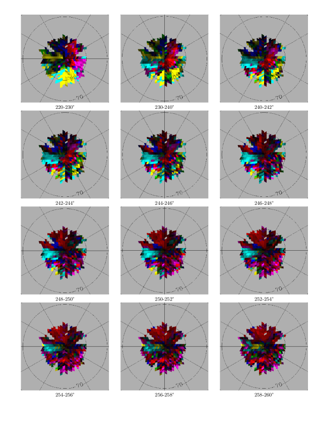
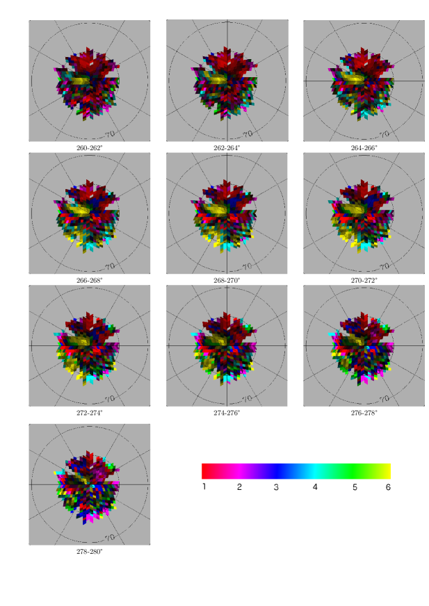
Facilities associated to HEALPix provide a means to represent each line of the PIDA or MIDA on a geographical map according to different projections. In particular the orthographic projection is the most suited among those available for the representation of the southern polar region of Mars. Prior to the mapping of the MIDA, we average along the Y dimension of the array all the valid values falling in a given solar longitude interval (of width 10° for the first two mosaics and then 2° for the following): LS=220-230°, 230-240°, 240-242°, and so on. In addition, subsequently to the mapping, we superpose on the map the position of the Seasonal South Polar Cap (SSPC) crocus lines as determined by Schmidt et al. (2009) at the beginning of each time interval of interest. As a result we obtain a series of 22 mosaics (at a spatial resolution of =64, i.e. 1.0°.pixel) that compiles the modelled version of the observations. Discussion of the results will be principally based on these mosaics. Map projections of the individual lines of the PIDA lead to one AOD map at a spatial resolution of =1024, i.e. 1/16°.pixel, for each OMEGA observation. A selection of these maps (Figures 12 to 16) is marginally examined to get some hints about the lowest latitudes and around the cap edge.
2.6 Classifying the seasonal trends of
Even though the modelling of the seasonal trend is performed in a pixel-wise manner, the spatial coherency of the time series of mosaics is excellent as can be seen in Figures 3 and 4. Then we may expect that in the MIDA, baselines can be gathered, based on similar shapes, into a limited number of classes. To test this hypothesis the whole collection of baselines is processed by kmeans classification provided by the R statistical package (http://www.r-project.org/). The main difficulty to overcome is the prior evaluation of the class number . For that purpose, several runs of the kmeans routine are conducted independently with an increasing value for this unknown input parameter. Then statistical tests Sugar and James (2003) are performed through the generation of a likelihood function depending on and peaking at the most likely value for the previous parameter. We found =4 though with a poor separability of the classes (inter-class variance only accounts for 32 % of the total variance of the data). This is to be expected when studying atmospheric conditions that transition progressively at the global scale of our investigation from one regime to the next. Nonetheless Figures 5 and 6 respectively demonstrate that a good spatial coherency and seasonal baseline separability is achieved for the four classes which boundaries must be considered as indicative only.
2.7 Assessing day-to-day variability and spatial heterogeneity
In Section 2.4 we define the variable component as the difference between the original signal and the mean trend respectively extracted from the PIDA and MIDA for the same (x,y) coordinates. We simply define an estimator of the day-to-day variability magnitude by calculating for each valid HEALPix bin the root mean square (RMS) of these differences over non-overlapping contiguous intervals of solar longitudes 10° in duration. By mapping the estimator in the geographical space according to the orthographic projection, six mosaics are obtained that indicate the most and least active locations for each time period (Figure 7). The relevance of the mosaics has been checked by comparing them to conjugated maps indicating the integrated number of original image pixels that falls into each bin of the PIDA for LS=220-230°, 230-240°, 240-250°, 250-260°, 260-270°, and 270-280°. No correlation is found for any of the time periods. In addition to producing mosaics, a spatial averaging of the estimator is performed separately over the four spatial regions conjugated to the classes distinguished in the previous Section resulting in distinct temporal trends (Figure 8 upper graph). As regards to spatial heterogeneity, we perform its assessment over the same four spatial regions. For that purpose we first calculate the root mean square of the variable component over a given region at each date, - time index - of the PIDA. We then obtain four temporal curves at full time resolution that are smoothed by a sliding average operation (width of the window: 10° LS). The result is then sampled at the solar longitudes 225°, 235°, 245°, 255°, 265°, and 275° (Figure 8 lower graph).
3 Trends of atmospheric dust opacity for the high southern latitudes
3.1 Main spatio-temporal units
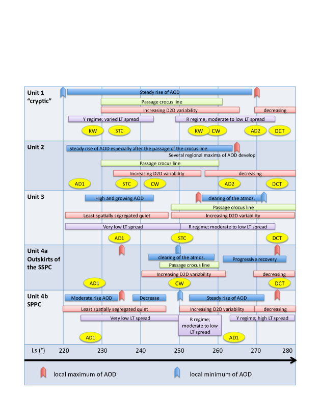
Figure 5 displays the contours of the four principal spatio-temporal units that have emerged from classifying the collection of seasonal trends followed by the dust optical depth. The first unit roughly spans the area between meridians 90°E and 210°E and parallels 70°S and 85°S. It corresponds basically to the portion of the southern polar layered deposits (SPLD) known as the “cryptic region” (see definition in Section 2.2). It is characterised by a steady rise of from 0.3 at the beginning of the covered period to a maximum 1.0 at LS=270°. The rate of increase is moderate for , before being accentuated. Once passed the maximum, one can observe a noticeable drop in the curve. Unit 2 is composed basically of two non contiguous area, the most extended being between meridians 210°E and 300°E and parallels 70° and 80°: Parva Planum, Argentera Planum. The eastern most part of the area is actually slightly deported towards the lower latitudes. The least extended area of unit 2 is centred around (78°S,100°E; western part of Promethei Planum). As regards to its temporal behaviour, this unit can be distinguished by a steady rise of that starts at higher values than unit 1 ( 0.5), has a significantly lower rate of increase, and reaches a maximum value of 0.9 ( at LS=265°). Then declines to some degree. Unit 3 is quite contiguous even though it displays a complex shape. The major part of it lies principally between longitudes 270°E and 30°E and at latitudes as high as 87°S and as low as 70°S including Dorsa Argentera. It also comprises the area occupied by the so-called Mountain of Mitchell located near 70°S, 40°E (James et al., 2000) and an “arm” of SPLD around the south permanent cap at longitudes between 120°E and 270°E. Units 2 and 3 basically coincide with the anti-cryptic region. The atmospheric opacity of unit 3 is already quite high at the beginning of our period of interest around 0.55, stays quite constant until LS=240°, and increases afterwards up to a maximum of 0.75 at LS=255°. Then it decreases down to a minimum of 0.6 at LS=272°. Our curve indicates the beginning of a reversal afterwards, but it is not possible to say if it is significant. Finally unit 4 surrounds the quasi totality of unit 3 as a “stripe” passing through (clockwise) the permanent cap and the nearby SPLD, the Argentera Planum, the Sisyphi Planum, and the Dorsa Brevia. A striking anti-correlation between the temporal behaviours of unit 3 and 4 can be noticed. Until LS=240°, the dust opacity remains basically at the same level (0.55) despite moderate rise for unit 4. Afterwards the baseline of the latter reaches its minimum ( 0.5 at LS=250° ) when the baseline of unit 3 reaches its maximum ( 0.75) and the other way around ( 0.8 at LS=275° for unit 4, 0.6 for unit 3).
3.2 Regional traits of AOD activity
The spatio temporal units with their distinct temporal signatures are the summarised expression of the dust loading of the atmosphere depicted with more details by the time series of mosaics built from the MIDA (explained in Section 2.5 and displayed in Figures 3 and 4). In addition one can appreciate the regression of the seasonal deposits by looking at the simultaneous displacement of the inner and outer crocus lines.
Cryptic region
When the latter region, which is nearly in a one to one correspondence to unit 1, is entirely covered by CO2 frost (), the overlying atmosphere AOD is the lowest of the entire seasonal cap. As the inner crocus line progresses through the region toward the high latitudes - faster than in any other longitude sectors - patches of more dusty atmosphere appear above the area that are just defrosted. By LS=254°, only the central part of the cryptic region displays AOD values below 0.5. Superimposed on the mean behaviour of steadily increasing opacity as noted above, we observe by LS=262° the emergence of a regional AOD maximum centred at (80°S,165°E) that grows in value and spatial extent and reaches its height at LS=272-274°, and starts to disappear afterwards but not completely. Thus this regional enhancement of dust opacity is present for at least 20 days. In the most western part of the cryptic region around the location (78°S,100°E; western part of Promethei Planum), there is an area of the same sort but that has been active even earlier (LS=230°). As result it is classified as belonging to unit 2 rather than to unit 1.
Anti-cryptic region
Unit 2 which falls principally in the latter region sees in many places a rise of atmospheric opacity since the beginning, i.e. even before the passage of the crocus lines. Defrosting has only a modest influence on the rise and several regional maxima’s develop. The most important one is along longitude 270°E and migrates by 5° towards the higher latitudes between LS=252° and LS=280°. Unit 3 is the portion of the seasonal cap that also shows relatively high and growing values of the overlying atmosphere AOD at least for . However contrary to unit 2, this trend then starts to reverse with the crossing of the inner crocus line. Consequently the subsequent prevalence of ice-free terrains seems correlated with a substantial apparent clearing of the atmosphere. At the end of the period of interest we observe a regional minimum of dust opacity around (75°S,330°E; Dorsa Argentera). We distinguish two sub-units for unit 4 (see Figure 5). At the lowest latitudes that we cover in the “anti-cryptic” sector (unit 4a) an early increase of AOD (modest in amplitude) followed by a decline is also observed linked to the passage of the inner crocus line. After LS=250-270° with the passage of the outer crocus line, the AOD starts to recover reaching 0.5 to 1 at the end of the period. Curiously, even though the region of the permanent cap (unit 4b) does not experience the crossing of the crocus lines, it displays a very comparable AOD seasonal baseline and thus has been also classified in unit 4 by the kmeans algorithm. Nevertheless this might just be a coincidence. To conclude one striking feature of the anti-cryptic region is thus the nearly continuous strip of relatively low AOD values (0.5-0.6) that accompanies the progressing transition zone between the inner and outer crocus lines after LS=262-264°. Such a propagating front explains the major characteristics of the temporal behaviour of units 3 and 4 and their anti-correlation.
3.3 Studying day-to-day variability and spatial heterogeneity
In Section 2.7 an estimator of the magnitude of the day-to-day variability is put forward and mapped at a resolution of 1.0°.pixel for six non-overlapping contiguous intervals of solar longitudes 10° in duration (220-230°, 230-240°, 240-250°, 250-260°, 260-270°, and 270-280°; Figure 7). The area where the resulting mosaics display meaningful values is more restricted in general than the area for which we have models of the mean trend of versus time. Indeed calculation of the estimator requires even more OMEGA observations per time intervals than for the model. Nevertheless this is not a limiting factor for studying the day-to-day variability poleward of 70°S latitude. For the variability is low (0.07) throughout the SSPC with a few exceptions. Then, passed LS 230°, the variability begins to rise very significantly (up to 0.3) in the “cryptic” sector at large (longitudes 60-240E°) regardless of the relative position of the considered bin with the inner crocus line. During the next time interval, such signs of intense low scale dust activity have intensified in the previous sector but have also propagated both clockwise and anti-clockwise. In the anti-cryptic sector enhanced values for the variance are confined within the transition zone. Inside the SSPC only the 0-60°E interval of longitudes remains relatively quiet. Then we reach the period () during which high variability is widespread among all sectors. Finally () the dust activity decreases in intensity especially inside the remaining SSPC and for latitudes equatorward of 75°S. Figure 8 illustrates the average seasonal evolution of the day-to-day variability (upper panel) and the seasonal evolution of spatial heterogeneity (lower panel) for each of the four units distinguished in Section 2.6. These graphs corroborate the previous examination. Furthermore they reveal that for each spatio-temporal unit has a very distinct signature. The atmospheric dust cover above the “cryptic” region (unit 1) displays the highest temporal variability in conjunction of being the second most spatially segregated. Nevertheless a look at Figure 6 reminds us that the absolute level of AOD is in general relatively lower than anywhere else. At the contrary above the “anti-cryptic” sector including the “Mountains of Mitchell” (unit 3) the dust cover is much more spatially uniform also implying a low day-to-day variability. According to the latter indicator alone, units 2 and 4 are intermediate. After LS 255° all units behave comparably to a first approximation.
3.4 Tracking local time dependencies
In this section our goal is to characterise local time dependencies of atmospheric optical depth during spring and beginning of summer for the high southern latitudes. In Section 2.3 we mention that an additional dimension can be optionally added to the PIDA by considering the local time of acquisition for each OMEGA pixel. A division of the martian sol into three equal Local Time (LT) intervals is adopted: 0-6, 6-12, and 12-18. Identically to what is described in Section 2.4 we model the mean trend of versus LS although each LT interval is now treated independently. As a result any systematic shift affecting the AOD correlated to the diurnal cycle should be dissociated from the variability associated to random estimation errors and day-to-day meteorology for example. The drawback of adding the LT dimension is that the number of samples per bin of the HEALPix grid is now much reduced. The bins for which enough points are available and sufficiently distributed in the period of interest fall predominantly poleward of the 80 parallel, the area that was scrutinised the most frequently by OMEGA. Finally the modelling leads to the generation of three MIDA, one per LT interval. Prior to further processing, we average along the Y dimension of each array all the valid values falling in the reference solar longitude intervals: LS=220-230°, 230-240°, 240-242°, etc. At this point quantifying the spread and the ordering of the triplet of seasonal values - one per baseline - is performed for each eligible bin and each LS range. In addition a better visualisation of the results is achieved by means of a special colour coding. We assign to each bin a distinctive primary hue and a luminosity depending on the ordering of the triplet and on its variance as follows. Red, magenta, blue, cyan, green, and yellow correspond respectively to the six possible ordering, i.e. permutations, among the three baselines. The luminosity is a continuous real number in the [0,1] interval that is set to . The denominator of the previous fraction represents three times the standard deviation of when doing the statistics on the whole dataset. By mapping our colour coded joint estimators of ordering and variance in the geographical space according to the orthographic projection we obtain a time series of mosaics (Figures 9 and 10). Bright and subdued colours indicate significant, respectively undetectable, LT variability. Table 1 summarises the local time pattern of dust activity for each color regime effectively realised in the series of mosaics.
| Colour regime | Local time pattern of dust activity |
|---|---|
| Yellow | |
| Magenta | |
| Red | |
| Cyan |
At the beginning of the covered period LS=220-230° a clear dichotomy separates the “cryptic sector” of longitudes with high diurnal variance and the “anti-cryptic” sector with much less pronounced values of . Nevertheless in both cases we observe two regimes: (magenta) in the western part (0-150°E) and (yellow) in the eastern part (150-300°E). The remaining area shows no sign of diurnal variability until LS 240°. During the period the portion of unit 1 (see Section 2.6) covered by the map stays predominantly in the yellow regime even though the middle part shows very low values of . Meanwhile closer to the pole over a quite extended area we rather have (“red” regime). In the interval a transition can be observed. Then for the predominance of the red regime is obvious everywhere except in the sector 240-270°E where the ordering remains in the regime (cyan) until . In any case the variance is moderate to low. After LS 264° and at least until LS 274° the yellow regime returns with quite high diurnal variability over the SPPC and for longitudes 180-240°E at the outskirts of the covered area. Past this date no clear spatially coherent trends are visible in the mosaics in terms of ordering nor in terms of spread.
3.5 Individual features
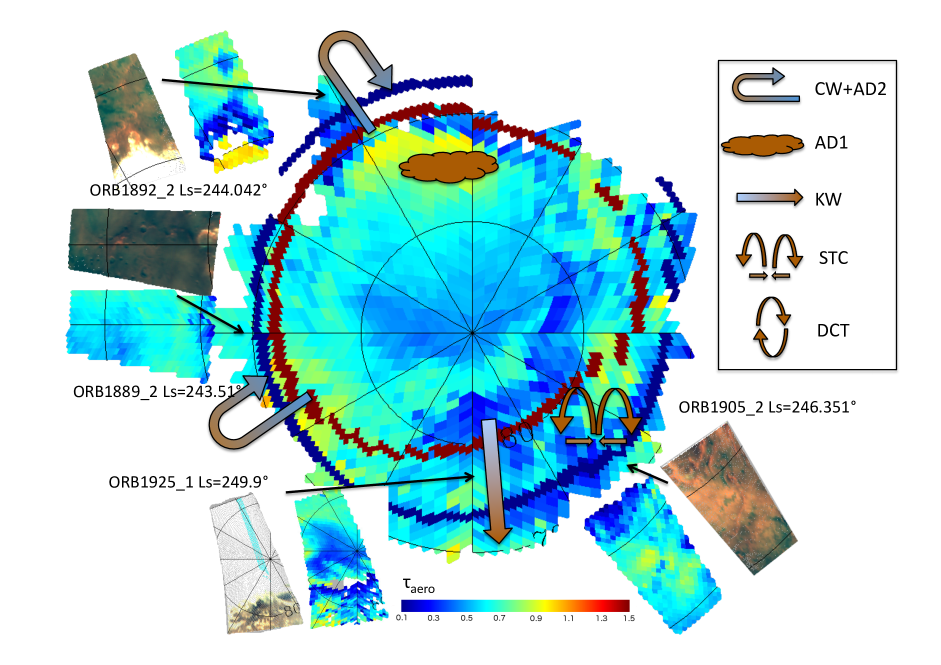
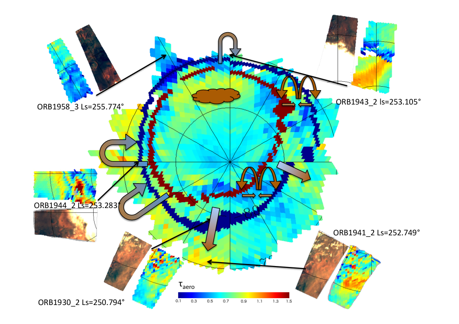
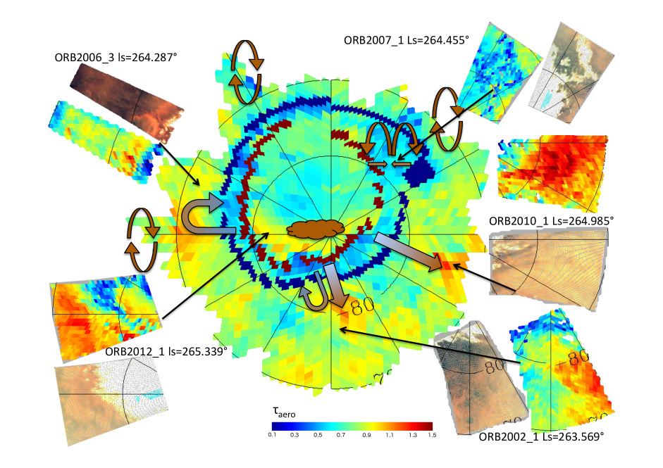
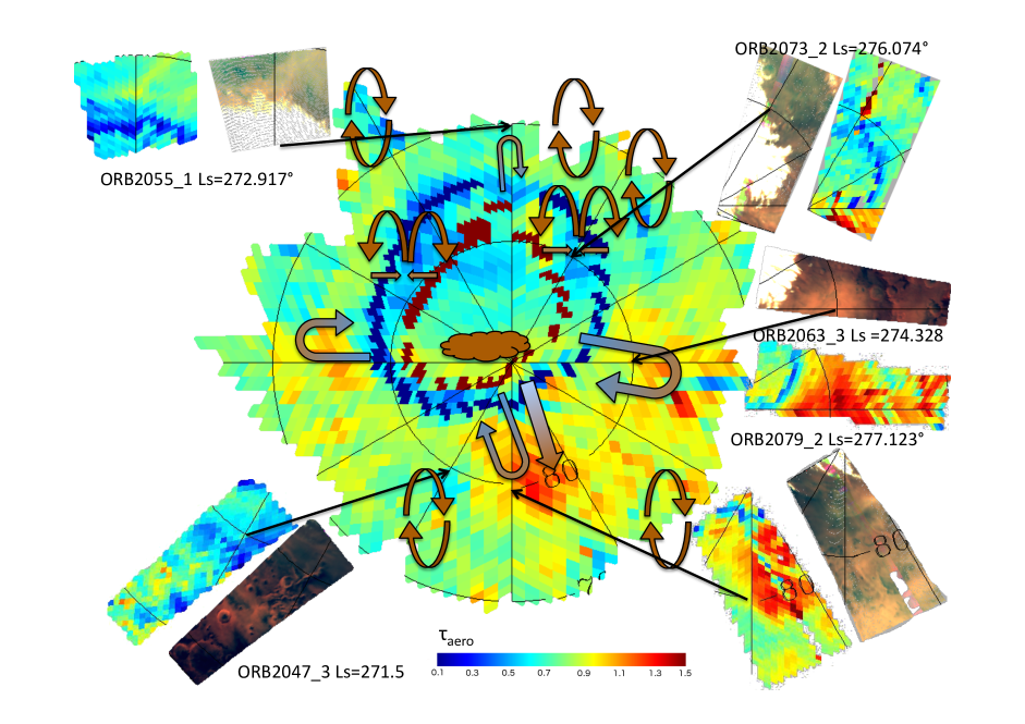
Further insights into the dust activity going on around the cap edge and at lower latitudes emerges from the examination of individual projected AOD maps (Section 2.5). Information provided by each map is enhanced by providing two companion maps associated to the same observation. In the first, an RGB composition of the top-of-atmosphere (TOA) martian reflectivity measured by OMEGA at three wavelengths (0.7070, 0.5508, and 0.4760 m) is shown. It is stretched so as to make visible the dust clouds as yellowish hues against mineral surfaces. Nevertheless it should be noted that such a stretch completely saturates the image over the the seasonal deposits. In the second map, a colour scale is used to indicate the local time of pixel acquisition. Figures 12 to 16 show a selection of nineteen observations out of the initial collection of 284 observations that illustrate different types of representative situations. In Figure 12 each observation corresponds to a line in a Table, the RGB composition, the AOD map, and the LT map being respectively arranged in the first, second and third column. In the other four Figures, each observation corresponds to the RGB composition and the AOD map alone, both superimposed on a context mosaic depicting the level of seasonal AOD. The pair is identified as well as situated in time (solar longitude Ls) and space (arrows). The following description is based on the entire collection of individual observations but illustrated with the selection.
In the interval 220-242° for which OMEGA provided global scale observations, we first note significant dust opacity’s around the cap (0.6-0.7) on the “morning” side and modest values on the “afternoon” side of the AOD maps (Fig.12b,c). This is corroborated by the visible images (Fig.12a). Then starting around 230° and lasting a least until 240° both the AOD maps (Fig.12e) and their visible counterparts (Fig.12d) reveal thick dust clouds mostly in the vicinity of the seasonal cap regardless of the local time (Fig.12f). It is worth mentioning that while the clouds are well outside the cap on the “morning” side, they penetrate well passed the transition zone on the “afternoon” side. After 240° until the end of the covered period, observations turn to more frequent but more spatially focused snapshots. The interval 242-255° is a period of usually quiescent activity in the afternoon for the defrosted area of units 1, 2, and 4a with low to moderate level of opacity ( 0.2-0.5; ORB1889_2, Fig.13, ORB1943_2, ORB1958_3 Fig.14). In the visible such a situation means a clear view of the surface brown features and low TOA reflectivities. Sometimes events of higher intensity ( up to 1.0) can be spotted (ORB1892_2, ORB1905_2, Fig.13). In the large transition zone of unit 1 the dust opacity retrieved by our method remains low while significant opacity is apparent in the visible images (ORB1925_1, Fig.13). A similar situation occurs at 250-275° for longitudes 0 to 60°E, unit 3 (ORB2007_1, Fig.15) From at least 250° to the end of the covered period ( 280°) marked opacity can be recognised around the cap with clear patterns depending on the spatio-temporal unit that this is considered. Once passed the crocus line, unit 1 (“cryptic region”) presents area of high atmospheric opacities that persist regardless of the local time. Nevertheless the highest values of occur more frequently during the second part of the “night” and in the morning (ORB2002_1, ORB2010_1, ORB2012_1, Fig.15, and ORB2079_2, Fig.16). Then surface features in the visible are subdued behind a diffuse veil of scattering aerosols with relatively elevated TOA reflectivities. Note that sometimes the development of the dust cloud is readily appreciable both in the AOD map and the RGB composition as in the pair of observations ORB1930_2, ORB1941_2, Fig.14 both acquired during the afternoon. For regions 2 and 4a the area close to defrosting area undergo locally intense dust activity (1-1.5) that are observed rather during the afternoon hours than during the early morning (ORB1944_2, Fig.14, ORB2006_3, Fig. 15, ORB2055_1, Fig. 16). A typical transient event captured by ORB2063_3 - a “storm” of local proportions - is shown in Fig. 16. One last observation driven by the examination of the dataset concerning units 2 and 4a is that the area that had been defrosted for 10° of solar longitude show low to moderate AOD corresponding to quite clear conditions in the visible images (ORB2047_3, Fig. 16).
3.6 Comparison with earlier works
In this last sub-section, we confront briefly the evolution and variability of the AOD given by on the one hand our study (OMEGA images in MY 27) and, on the other hand, by the study of Toigo et al. (2002); Imamura and Ito (2011) (TES and MOC images in MY 24, 25 and 26 ).
Basically Toigo et al. (2002) present two (TES) maps of dust opacity at 9 µm. In addition they also discuss a discontinuous series of MOC daily global mosaics in color. The first TES map depicts the situation at Ls 228° in which infrared opacity can be in excess of 0.5 all around the edge of the polar cap while it remains between 0.1 and 0.2 at lower latitudes (background level). This is the expression in the infrared of what is depicted more qualitatively but with more spatial details by a MOC mosaic. Typically a dust cloud is created near the edge of the polar cap, is blown away from the cap while growing in extent, and then dissipates over a period of 6-8 hours. In particular at LS228° a number of discrete well-defined dust clouds can be seen everywhere around the cap edge, especially in the 180-270°E longitude sector. Our AOD maps generated from individual observations taken by OMEGA at the beginning of the period of interest ( cover large strips of Mars, joining across the cap areas of opposite longitudes at moderate latitudes (Section 3.5). The regions external to the cap (latitudes equatorward of 70°S that are not visible in our mean trend mosaics, Fig.12) indeed display extended cloud systems following LS 225° for varied longitude sectors, regardless of local time. Nonetheless due to the limited time and spatial coverage of the subsequent OMEGA observations, it is not possible to monitor the propagation of transient dust clouds from the cap edge to the lower latitudes.
In the second TES map at Ls 257.5° significant accumulation of dust is restricted to the longitudes from 270 to 45°E. At contrary the most productive area in our case around LS 255-260° of MY 27 is in the longitude sector 180-300°E (unit 2), rather in agreement with the results of Imamura and Ito (2011) (see below).
The work of Imamura and Ito (2011) led to a more systematic mapping of the dust at 9 µm. For Martian Year (MY) 24, Ls=270-280°, a global map displays an elongated dusty region that encircles the south pole with a gap in the range 330-60°E; this feature was also observed in MY 25 and 26. The map is part of a larger study that also addresses the temporal and spatial variation of the 9 µm dust optical depth in this region using Hovmöller diagrams for three Martian years. For the range of solar longitudes , Imamura and Ito (2011) found that dust clouds emerge repeatedly (every 10-20 sols) from an area delimited by latitudes 70–80°S and longitudes 240–300°E. Then they move westward and reach the region in the longitude sector 60–120°E to finally disappear. The overall longitude range of the disturbance, 60–300°E, coincides with elevated terrains in the south polar region, and with the increase of dust optical depth observed at Ls=270-280° that encircles the south pole. The quasi-periodic behaviour (period of 10–20 sols) of the dust optical depth disturbance that is recognised in the latitude band 70-80°S by Imamura and Ito (2011) in their Hovmöller diagrams is absent from our curves of seasonal AOD even for the main source regions (Unit 2 until LS250°, then Unit 1).
To summarise, even though similar broad tendencies arise from the different studies at certain dates and for certain regions, discrepancies are the rule. Inter-annual variability and notable differences in terms of resolutions can account for this situation.
4 Discussion
Figure 11 proposes a qualitative summary of the principal results obtained in Section 3. The four main spatio-temporal units are followed in parallel according to the solar longitude. In addition we indicate which time interval is concerned by the passage of the crocus lines. A series of indicators - the seasonal trend of (Section 2.4), the day-to-day variability and spatial heterogeneity (Section 2.7), as well as the ordering and spread of the triplet of baseline values (Section 3.4) are reported. In the present section these indicators are now conjointly discussed. The goal here is to propose scenarios, i.e. succession in time of mechanisms or conditions that plausibly control the atmospheric dust activity for different area of the high southern latitudes in spring. First we introduce several mesoscale and microscale circulation processes based on earlier works. Then the expression, expected conditions of occurrence, and dust lifting capabilities of such processes are phenomenologically linked with the evolution and variability of the AOD observed with OMEGA in conjunction with the state of the regressing seasonal cap. This is the method by which we put forward hypotheses regarding which circulation process(es) likely control the atmospheric dust activity for a given unit and for a given time range. These proposed scenarios, which are illustrated by a series of figures (13 to 16), could be tested by future high-resolution atmospheric mesoscale modelling.
4.1 Introducing several mesoscale and microscale circulation processes.
- Katabatic Winds
-
(KW) are drainage atmospheric flows that form in the lowest atmospheric levels ( one hundred meters) when cooled dense air is accelerated down sloping terrains by gravity, overcoming the opposing along-slope pressure gradient. Martian conditions conducive to this behaviour are the extremely low temperatures of the seasonal deposits in thermodynamical equilibrium with the overlying CO2 gas and nighttime radiative cooling of surface and atmosphere. In both cases they are maximum at night hours when the temperature inversion above surfaces is the highest (Spiga, 2011; Kauhanen et al., 2008).
- Thermal Circulations
-
are triggered by lateral temperature heterogeneities due to soil thermophysical contrasts but most importantly due to icy vs. bare surface contrasts. They can cause high surface friction and vertical mixing thus injecting dust in the atmosphere (Spiga and Lewis, 2010; Siili et al., 1999). Atmospheric flow modellings (Holton, 2004) demonstrate that a rough proportionality exists between the typical size of the temperature heterogeneities and the height reached by the convection cells. Note that the latter own a dynamical surface branch oriented from the lowest to the highest temperatures and a return flow, i.e. blowing in opposite direction, at higher altitude. In particular Toigo et al. (2002) have studied the development of the so-called cap winds (CW), analogues to terrestrial sea breeze circulation, generated by the strong thermal contrasts that exist along the retreating edge of the southern spring polar cap during the middle to late spring. Their three-dimensional numerical modelling at mesoscales demonstrate that surface wind stresses are sufficient at some location during specific local time intervals to initiate movement of sand-sized particles and hence dust lifting over quite large area. Thus they recognise cap edge winds, a mesoscale structure ( km), as an important factor for the development of dust storms near the cap edge. However the influence of a having a gradual transition between the inner and outer crocus lines instead of a neat cap edge and the availability of dust and/or sand particles are not addressed in their paper.
Note that Siili et al. (1999) performed a set of numerical experiments with the two-dimensional Mars Mesoscale Circulation Model that shed some new light about the previous two processes. In particular they demonstrate that strong near surface winds potentially capable of lifting dust from the surface can be achieved (i) in daytime along a slope which lower section is frozen and upper section is ice-free: “anabatic winds” (ii) in nighttime over a fully ice-covered slope or defrosted in its lower section: “katabatic” winds. Inclusion of atmospheric dust ( = 0.3) reduces the daytime ice-edge forcing - the upslope flow is attenuated - while the nocturnal downslope flow is enhanced. Consequently thermal circulations, in the form of anabatic winds, can be enhanced by local relief in the defrosting area. Interestingly, spatial segregation of frozen and ice free terrains in this transition zone can be controlled by topography through slope orientation and profile for example.
- Daytime Convective Turbulence
-
(DCT) is particularly well developed in the Martian boundary layer during the afternoon under the influence of the heated surface. Even in situations of weak large-scale and mesoscale winds, this thermally-driven convection might itself cause significant vertical mixing and wind gustiness. Two worth-mentioning manifestations of convective turbulence are “convective gusts” found near walls of convective cells and convective vortices linked with “dust devils”.
- Synoptic Scale Circulation
-
at large-scale (>100s kilometers) is characterised by inter-hemispheric meridional Hadley Cells and mid-latitude baroclinic waves, the latter features occasionally accompanied by dust fronts extending over thousands of kilometers.
4.2 Unit 1
For unit 1, that well corresponds to the “cryptic” region, we distinguish four successive phases of activity.
In the very early phase of defrosting (), the seasonal AOD is the lowest of the entire seasonal cap, and we have (i.e. a “yellow regime”) with dispersed values of , meaning that, statistically, there is more dust in the atmosphere during the early hours than during the morning and the afternoon with local variations of the spread. For the mantle of seasonal CO2 deposits is still quite continuous and exhibits a very compact texture in the form of a translucent slab (Kieffer et al., 2000). Nonetheless it is then superficially contaminated by a large amount of dust making it barely detectable by its spectral signature in the shortwave infrared (Langevin et al., 2006). We put forward the hypothesis that powerful katabatic winds (KW) hurtling down existing topographical slopes up to couple hundreds meters above the surface likely cause high surface stresses, lifting the dust that contaminates the ice. At the same time these winds likely evacuate the dust downstream in the form of dust clouds lying low in the atmosphere leading to an under-estimated optical depth by our method (Douté et al., 2013). By the same token we could also explain the fast superficial cleaning undergone by the CO2 icy deposits at the ground as noted by Langevin et al. (2006) between . As for the requirement of significant slopes, we find in the area the mouth of two chasma and the south polar layered deposits display their most pronounced scarps down to the surroundings plains. The katabatic mechanism would be especially efficient for .
In the next phase, starting at LS 240°, we observe a steady rise of seasonal AOD in association with an increasing day-to-day variability. Conjointly for a transition between the “yellow” and “red” regimes occurs. That means that, thereafter, the AOD is statistically higher during the afternoon than during the morning and more so than during the early hours with low to moderate spread (see also section 3.4 and Table 1 for further descriptions). Despite the growing activity of the second phase, the increase of seasonal AOD is late compared to unit 2. This is somewhat surprising since unit 1 is the sector for which the inner crocus line is progressing the fastest. Our interpretation relies on the fact that, with the wide separation between the inner and outer crocus lines, spatially segregated defrosting patterns cover a very extended area for the considered time period (Schmidt et al., 2009). As a consequence during daytime, and at the kilometre scales (small scales), local temperature contrasts are huge promoting thermal circulations but limited in their vertical extent. They become stronger with LT injecting more dust during the afternoon. Besides during nighttime, because of reduced lateral thermal contrasts and temperature inversions above high-standing icy surfaces, the katabatic wind regime could recover for a few hours sweeping the dust downstream. Conjunction of the two phenomena - katabatic winds (KW) much more efficiently than small scale thermal circulation (STC) - restrict atmospheric upward mixing and dust accumulation above the region to some degree.
By LS 260° the area corresponding to unit 1 is entirely defrosted. Higher in latitude the separation between the inner and outer crocus lines is shrinking. Despite the decline of strong lateral thermal contrasts, we have the emergence of a persistent regional AOD maximum that grows in value and spatial extent and reaches its peak at LS=272-274°. That corresponds to the maximum level of mean seasonal AOD for the unit which is then also the most spatially segregated in terms of . Unit 1 evolves from a red regime to a regime for which the night hours display significantly higher AOD than during daytime even though opacities stay persistently at high level in agreement with the individual observations (Section 3.5). These elements forge the following assumption for the third phase. The conjunction of two mechanisms for atmospheric dust enhancement in the region could be envisioned. The advection and upward diffusion (AD2) of dust from the retreating distant edge of the cap is the first potential mechanism. As explained before preferentially katabatic winds but also possibly cap edge winds (CW) both able to carry dust blow outward from area at higher latitudes that are still in the second phase. Thermal gusts and dust devils associated to the daytime convective turbulence (DCT) (Spiga, 2011; Spiga and Lewis, 2010) is the second potential mechanism.
The fourth and last phase corresponds to the decline of seasonal AOD after LS 270° with the related diminishing day-to-day variability or, equivalently, spatial heterogeneity. At this point the crocus line is remote from the “cryptic” region and has stopped being a source of dust. Hence the thermal gusts and dust devils which persist exclusively are the best explanation for moderately efficient dust lifting and upward transport.
4.3 Unit 2
For unit 2 we distinguish three successive phases of activity.
The first one stretches from the beginning of the covered period to LS 235-240° when the region is still entirely covered by the seasonal CO2 deposits. From a starting value of 0.5 the mean AOD steady grows regardless of the crocus date (see definition in section 2.2) in many places which are spatially coherent in their behaviour. Therefore we suggest that the advection of dust at high altitude (AD1) from the lower active latitudes is the main origin of the increasing atmospheric opacity. Meteorological maps (not included here) of wind intensity and direction were extracted from GCM simulations (Forget et al., 1999) for the southern high latitudes (60°S) and examined. They show that poleward air fluxes at synoptic scales are well developed between 5 and 11 km at this season and nearly reach the pole. Such fluxes correspond to the return branch of a large scale convection cell that is established between the cold cap and the surrounding warming ice free terrains. Due to orographic differences or due to the different extent of the transition zone, this synoptic feature could be more strongly established at the longitudes of unit 2 than at those of unit 1. Indeed the situation differ markedly between the two units during this early period.
During the second phase the climb of seasonal AOD levels continues at the same overall rate while the crocus lines sweep the unit. The defrosting area that presents a geographical mixture of ice-free and still frozen terrains implying high thermal contrasts is more limited in extent than for unit 1, of the order of 2 to 5° in latitude. Day-to-day variability is also progressively on the rise with greatest values in the defrosting area. Meanwhile several regional maxima develop after the passage of the crocus line, and the peak of atmospheric opacity due to aerosol is reached at LS 265°. We put forward the hypothesis that unit 2 shares common processes with unit 1, those prevailing during the second and third phases of the latter, with one crucial difference. Similarly to unit 1, we have in the defrosting area daytime dust lifting associated to small scale thermal circulation (STC). Contrary to unit 1, where topography allows for nighttime katabatic winds, the only mechanism to blow efficiently dust downstream are the daytime thermal cap winds (CW) that could be established at the mesoscales between the SSPC and the defrosted terrains. Indeed they likely allow to some extend vertical diffusion and transport (AD2) of dust in the atmosphere towards the lower latitudes that are entirely defrosted. The whole scheme is compatible with the examination of the individual OMEGA images that indicate the occurrence of most transient dust events during the afternoon in this region.
In the third phase, when the outer crocus line definitively leaves unit 2, declines soon followed by the seasonal level of AOD. Such a behaviour, equivalent to phase 4 of unit 1, has likely the same origin: less efficient dust lifting by gusts and dust devils (DCT).
4.4 Unit 3
This unit is characterised by a first phase of gradually enhanced dust opacity rather similar to the one experienced by unit 2 until LS 250°. The difference resides in the fact that before LS 245°, the atmospheric dust layer is more uniform than anywhere else especially in the area of the “Mountain of Mitchell”. As a consequence, the day-to-day variability is also very low and no signs of local time dependencies (at least for the highest latitudes) can be noted. The advection of dust by the synoptic circulation (AD1) from active area at lower latitudes is probably the main origin for the increasing atmospheric opacity with no contribution of a local activity because all the unit is still frozen during this phase.
The situation starts to change after LS 250° with the gradual sweeping by the crocus lines, the day-to-day variability that becomes significant, and the emergence of a “red” regime - dust activity more significant in the afternoon- associated to moderate to low spread regarding the behaviour of AOD as a function of local time. In the defrosting area, a relative clearing of the atmosphere is observed especially since the inner and outer crocus lines are well separated (LS 255°). The clearing sometimes spreads beyond the principal outer crocus line particularly for in the area of the “Mountain of Mitchell” (then in their last phase of defrosting) and around Dorsa Argentera around LS 275°. As for the cryptic region in its second phase, the geographical mixture of ice-free and still frozen terrains should logically imply local high thermal contrasts in turn promoting intense but small scale thermal circulation (STC). The latter would then be in phase with the diurnal cycle and provide enough surface stresses to raise the dust (Toigo et al., 2002). However dust clouds are not detected at significant level by our method nor they are clearly apparent in the RGB compositions produced from the visible OMEGA images. These convergent observations strongly support the view of a quiet dust activity in the transition zone and beyond. Note that, unlike what goes on in unit 1 during phase 2, the katabatic winds cannot take over since no significant slopes can be found at the regional scale in the longitude sector of unit 3. Furthermore the cap winds could also be inhibited by the broad width of the transition zone, i.e. the absence of a sharp thermal boundary of regional proportions. The previous elements converge so as to limit dust opacity around the SSPC in unit 3 even though it gradually increases.
4.5 Unit 4
We think that this unit can be divided into two sub-units each one being characterised by specific mechanisms despite their very comparable but likely coincidental behaviour. Sub-unit 4a mainly corresponds to the lowest latitudes that we cover in the “anti-cryptic” sector whereas sub-unit 4b lies basically in the region of the south permanent polar cap (SPPC).
Sub-unit 4a very much behaves like unit 3 but in advance of seasonal phase. In the period advection of dust at high altitudes from the lower latitudes is the preferred mechanism for explaining relatively high AOD levels. Around LS 250° with the passage of the crocus line, an apparent local minimum of seasonal AOD is reached because of the limitations of our method. Cap edge winds likely blow across the relatively narrow transition zone lifting the dust but not mixing it high enough for the AOD to be correctly estimated. Thereafter a progressive and marked rise of dust opacity intervenes (from 0.55 to 0.8) that we attribute to the advection of dust by the cap winds blowing from the defrosting area that is moving away. Then the thermal winds fade gradually to be replaced by gusts and dust devils of the DCT.
For sub-unit 4b the initial rise of seasonal AOD until LS 235° and then decline down to 0.5 at LS 250° shows no signs of local time dependencies nor appreciable low day-to-day variability. This conjunction of factors supports the hypothesis that dust opacity is then controlled by large scale dynamics transporting dust high in the polar atmosphere. By LS 250° the atmosphere above the SPPC sees a strong and continuous enhancement of seasonal AOD. Meanwhile we observe an increasing then a decreasing day-to-day variability, the latter evolution being well correlated with the trends affecting the same indicator for the “cryptic” region. As far as the local time dependencies are concerned we are rather in a “red” regime (AOD is statistically higher during the afternoon than during the morning and more so than during the early hours) with modest spread. Therefore we suggest that the SPPC undergoes the influence of units 1 and 2 activity by migration of dust clouds toward the pole at altitudes of a few kilometres thanks to the return flow of the thermal cap winds (Section 4.1). Influence of unit 3 and 4a might be more reduced due to the relative inhibition of the mesoscale thermal winds as evoked earlier.
5 Summary
The OMEGA instrument has acquired a comprehensive set of observations in the near-infrared (0.93-5.1 microns) at the high southern latitudes of Mars from mid-winter solstice (LS=110°, December 2004, MY 27) to the end of the recession (LS=320°, November 2005). We systematically process a subset of these observations from LS=220° to 280° by performing the inversion of radiative transfer schemes described in Douté et al. (2013) and Vincendon et al. (2008) on every top of the atmosphere reflectance spectra forming the OMEGA images. As a result, we obtained a series of maps depicting the distribution of aerosol optical depth (AOD) noted . The maps were normalised in order to correct for changes due solely to varying atmospheric height because of topography. They were independently integrated into a common grid generated from the Hierarchical Equal Area isoLatitude Pixelization of Mars southern hemisphere. Such an integration, that can be performed at different spatial resolutions, allows to build the time evolution of the AOD for each spatial bin of the HEALPix partition. We then separate two contributions: a mean trend of versus time, i.e. the baseline, and a highly variable component, i.e. the day-to-day variability around the baseline with an adapted method. We also implement a data processing to isolate any dependencies to the local time (diurnal cycle) of a given bin. The HEALPix system provides means to map the values of atmospheric opacity or of any derived quantity for a certain date or averaged over a time interval according to different geographical systems. Thus we generate time series of orthographic mosaics depicting spatio-temporal distribution of the seasonal mean values, the variance and the local time dependence of the AOD. Besides, although the modelling of the seasonal trend is performed in a pixel-wise manner, the spatial coherency of the mosaics is excellent. Then we may expect that seasonal baselines can be gathered, based on similar shapes, into a limited number of classes. This was confirmed by performing a kmeans classification that gives four main types of seasonal trends followed by the AOD in four units segmenting the southern polar region. Following this complete analysis of the data , each spatio-temporal unit was studied carefully for searching trends of atmospheric dust opacity.
As a result a synthetic view (Figure 11) of dust activity in the south polar atmosphere in mid spring to early summer has been established. From this compilation of observations we propose hypothesis regarding the origin of aerosol activity of the southern polar region. Different mechanisms are invoked at a variety of spatial scales in conjunction with the regression stage reached by the seasonal deposits. In particular we suspect that two mechanisms might play a major role for lifting and transporting efficiently mineral particles and create dust events or storms: (i) nighttime katabatic winds (KW) at locations where a favourable combination of frozen terrains and topography exists (e.g. unit1, ) (ii) daytime mesoscale thermal circulation at the edge of the cap, i.e. cap winds (CW), when the defrosting area (transition zone) is sufficiently narrow (e.g. unit2, ). Indeed this kind of breezes could be inhibited, should the width of the transition zone be broad, i.e. in the absence of a sharp thermal boundary of regional proportions (e.g. unit4a, ). Thermal circulation at smaller scales (STC) due to the high thermal contrasts associated to segregated terrains in the transition zone exist and could also pick up some dust but likely leads to limited vertical and horizontal transport (e.g. unit3, ). Far from the seasonal cap, gusts and vortexes associated with Daytime Convective Turbulence (DCT) over ice-free terrains may not be an efficient mechanism to inject large amount of dust in the atmosphere explaining the clear decline of the AOD after LS 270° for the whole south polar region. Inside the seasonal cap, advection of dust at high altitude from the lower active latitudes is likely the main origin of the increase of the seasonal atmospheric opacity around LS 235°, then LS 275°.
As regards to the production of atmospheric dust in the defrosting area, the sector with the highest AOD values/variability/increase spans longitudes 180-300°E (unit 2) around LS 250°. Later (LS 267°) the situation has changed drastically and the cryptic sector becomes the most productive while the longitude sector 300-60°E (unit 4a and 3) remain moderately dust-generative.
Our work thus contributes to understanding the sequence of phenomena that control dust activity in the south polar atmosphere and suggests complex interaction between them. It calls for new simulations of the martian surface-atmosphere dynamics at mesoscales (between 1000 km and 1 km) considering topographical effects to reproduce the observations and to confirm the interpretations. In particular taking into account the gradual defrosting between the inner and outer crocus lines instead of considering a neat cap edge is of primordial importance. The local and regional availability of dust and/or sand particles needs to be addressed as well. Finally the possible interference of the baroclinic wave system with the convection cell that is established between the cold cap and the surrounding warming ice free terrains - including low altitude cap winds and high altitude return flows - must also be modelled properly.
Acknowledgements
We thank the OMEGA team at Institut d’Astrophysique Spatiale for support with sequencing and data downlink activities. This work is supported by a contract with CNES through its Groupe Système Solaire Program. We are grateful to X. Ceamanos and A. Spiga for their reading of the manuscript and for fruitful discussions. We would like to warmly thank both anonymous reviewers for their tremendous work in reviewing the article and their constructive comments.
References
- Basu et al. (2004) Basu, S., Richardson, M.I., Wilson, R.J., nov 2004. Simulation of the Martian dust cycle with the GFDL Mars GCM. Journal of Geophysical Research (Planets) 109 (E18), 11006–+.
- Chang and Lin (2011) Chang, C.-C., Lin, C.-J., 2011. LIBSVM: A library for support vector machines. ACM Transactions on Intelligent Systems and Technology 2, 27:1–27:27, software available at http://www.csie.ntu.edu.tw/~cjlin/libsvm.
-
Douté et al. (2013)
Douté, S., Ceamanos, X., Appéré, T., 2013. Retrieving atmospheric dust
opacity on mars by imaging spectroscopy at large angles. Planetary and Space
Science 85 (0), 38 – 52.
URL http://www.sciencedirect.com/science/article/pii/S00320%63313001347 - Forget et al. (1999) Forget, F., Hourdin, F., Fournier, R., Hourdin, andTalagrand, C., O., Collins, M., Lewis, R., S., Read, andHuot, P. L., J., oct 1999. Improved general circulation models of the Martian atmosphere from the surface to above 80 km. J. Geophys. Res. 104 (.13), 24155–24176.
- Forget et al. (2006) Forget, F., Millour, E., Lebonnois, S., Montabone, L., Dassas, K., Lewis, S. R., Read, P. L., López-Valverde, M. A., González-Galindo, F., Montmessin, F., Lefèvre, F., Desjean, M.-C., Huot, J.-P., Feb. 2006. The new Mars climate database. In: Mars Atmosphere Modelling and Observations. pp. 128–+.
- Górski et al. (2005) Górski, K. M., Hivon, E., Banday, A. J., Wandelt, B. D., Hansen, F. K., Reinecke, M., Bartelmann, M., Apr. 2005. HEALPix: A Framework for High-Resolution Discretization and Fast Analysis of Data Distributed on the Sphere. ApJ622, 759–771.
-
Holton (2004)
Holton, J. R., 2004. An introduction to dynamic meteorology. International
geophysics series. Elsevier Academic Press, Amsterdam, Boston, Heidelberg,
Ch. 5, pp. 115–138, sommaire disponible en ligne
http://www.sciencedirect.com/science/publication?issn:00746142&volume:88.
URL http://opac.inria.fr/record=b1122647 - Horne and Smith (2009) Horne, D., Smith, M. D., Mar. 2009. Mars Global Surveyor Thermal Emission Spectrometer (TES) observations of variations in atmospheric dust optical depth over cold surfaces. Icarus200, 118–128.
-
Imamura and Ito (2011)
Imamura, T., Ito, Y., 2011. Quasi-periodic dust events in the summertime south
polar region of mars. Icarus 211 (1), 498 – 503.
URL http://www.sciencedirect.com/science/article/pii/S00191%03510003209 - James et al. (2000) James, B., P., Cantor, A., B., Malin, andEdgett, M. C., andCarr, K., H., M., Danielson, E., G., Ingersoll, P.andDavies, A., E., M., Hartmann, K., W., McEwen, S.andSoderblom, A., A., L., Thomas, C., P., Veverka, J., apr 2000. The 1997 Spring Regression of the Martian South Polar Cap:Mars Orbiter Camera Observations. Icarus 144, 410–418.
- James et al. (2001) James, P. B., Cantor, B. A., Davis, S., 2001. Mars orbiter camera observations of the martian south polar cap in 1999 - 2000. J. Geophys. Res. 106 (E10), 23635 – 23652.
- Kahre et al. (2006) Kahre, M. A., Murphy, J. R., Haberle, R. M., Jun. 2006. Modeling the Martian dust cycle and surface dust reservoirs with the NASA Ames general circulation model. Journal of Geophysical Research (Planets) 111, 6008.
- Kauhanen et al. (2008) Kauhanen, J., Siili, T., Järvenoja, S., Savijärvi, H., Sep. 2008. The Mars limited area model and simulations of atmospheric circulations for the Phoenix landing area and season of operation. Journal of Geophysical Research (Planets) 113, 0.
- Kieffer et al. (2000) Kieffer, H. H., Titus, T. N., Mullins, K. F., Christensen, P. R., 2000. Mars south polar spring and summer behavior observed by TES: Seasonal cap evolution controlled by frost grain size. J. Geophys. Res. 105 (E4), 9653 – 9700.
-
Korablev et al. (2005)
Korablev, O., Moroz, V., Petrova, E., Rodin, A., 2005. Optical properties of
dust and the opacity of the martian atmosphere. Advances in Space Research
35 (1), 21–30.
URL http://www.sciencedirect.com/science/article/B6V3S-4BWW%9G6-16/2/f5cd1e548973751ba6a1295551360088 - Langevin et al. (2007) Langevin, Y., Bibring, J.-P., Montmessin, F., Forget, F., Vincendon, M., Douté, S., Poulet, F., Gondet, B., Jul. 2007. Observations of the south seasonal cap of mars during recession in 2004-2006 by the omega visible/near-infrared imaging spectrometer on board mars express. J. Geophys. Res. 112, –.
-
Langevin et al. (2006)
Langevin, Y., Doute, S., Vincendon, M., Poulet, F., Bibring, J.-P., Gondet, B.,
Schmitt, B., Forget, F., Aug. 2006. No signature of clear co2 ice from the
/‘cryptic/’ regions in mars’ south seasonal polar cap. Nature 442 (7104),
790–792.
URL http://dx.doi.org/10.1038/nature05012 - Schmidt et al. (2009) Schmidt, F., Douté, S., Schmitt, B., Vincendon, M., Bibring, J.-P., Langevin, Y., The OMEGA Team, Apr. 2009. Albedo control of seasonal South Polar cap recession on Mars. Icarus 200, 374–394.
-
Siili et al. (1999)
Siili, T., Haberle, R. M., Murphy, J. R., Savijarvi, H., 1999. Modelling of the
combined late-winter ice cap edge and slope winds in mars hellas and argyre
regions. Planetary and Space Science 47 (8-9), 951 – 970.
URL http://www.sciencedirect.com/science/article/pii/S00320%63399000161 - Spiga (2011) Spiga, A., Aug. 2011. Elements of comparison between Martian and terrestrial mesoscale meteorological phenomena: Katabatic winds and boundary layer convection. Planet. Space Sci.59, 915–922.
- Spiga and Lewis (2010) Spiga, A., Lewis, S. R., 2010. Martian mesoscale and microscale wind variability of relevance for dust lifting. International Journal of Mars Science and Exploration 5, 146–158.
-
Sugar and James (2003)
Sugar, C., James, G., 2003. Finding the number of clusters in a dataset.
Journal of the American Statistical Association 98 (463), 750–763.
URL http://www.tandfonline.com/doi/abs/10.1198/016214503000%000666 - Toigo et al. (2002) Toigo, A. D., Richardson, M. I., Wilson, R. J., Wang, H., Ingersoll, A. P., Jul. 2002. A first look at dust lifting and dust storms near the south pole of Mars with a mesoscale model. Journal of Geophysical Research (Planets) 107, 4–1.
- Vapnik (1998) Vapnik, V., 1998. Statistical Learning Theory. Wiley, New York.
- Vincendon et al. (2008) Vincendon, M., Langevin, Y., Poulet, F., Bibring, J.-P., Gondet, B., Jouglet, D., OMEGA Team, Aug. 2008. Dust aerosols above the south polar cap of Mars as seen by OMEGA. Icarus 196, 488–505.
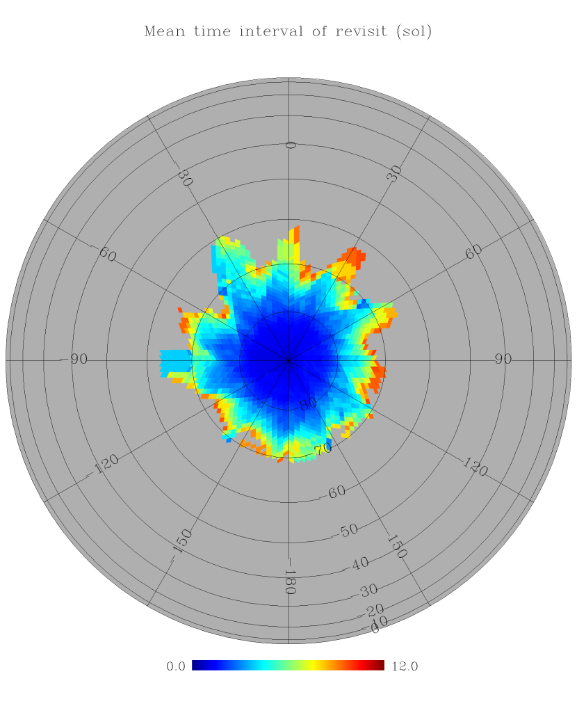
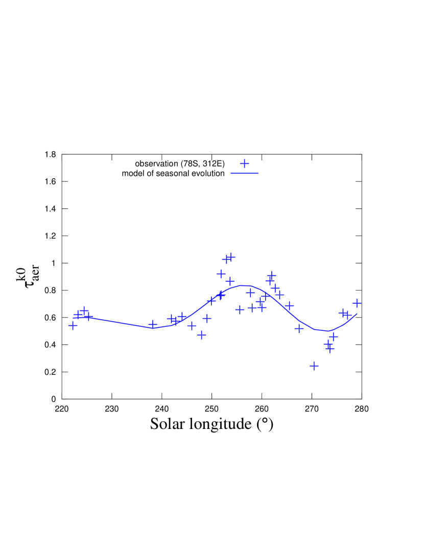
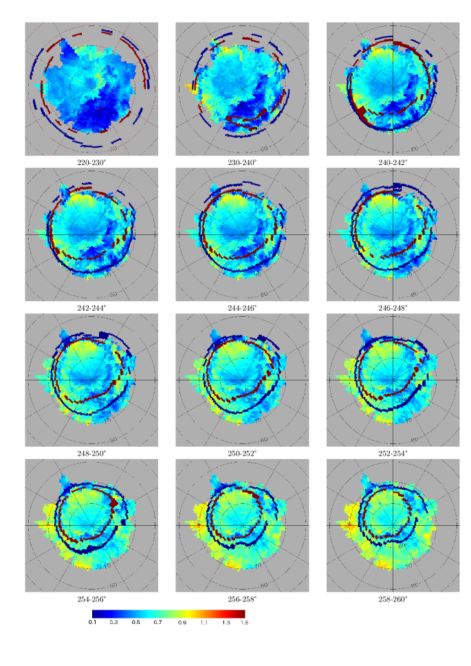
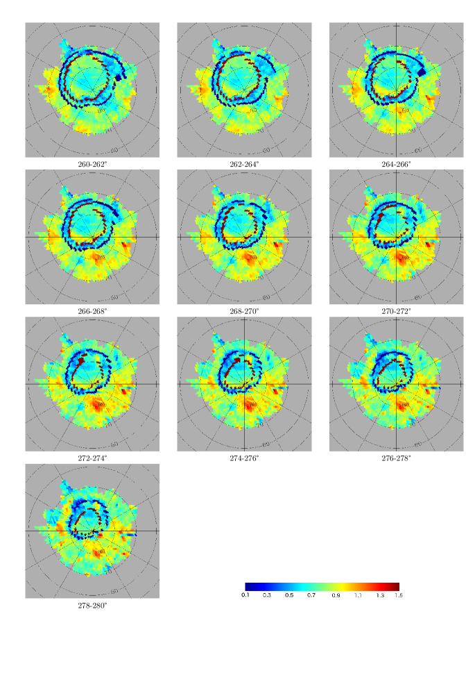
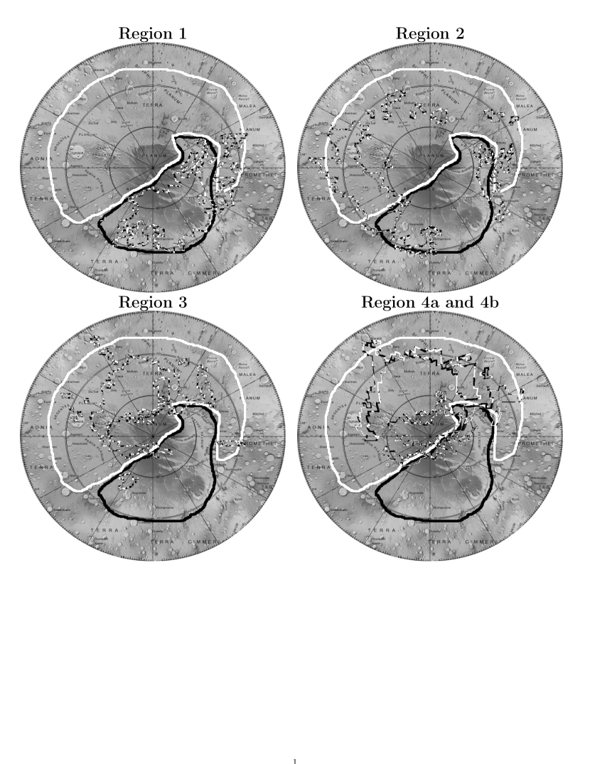 |
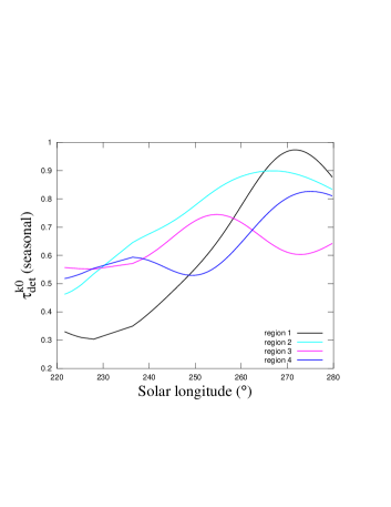
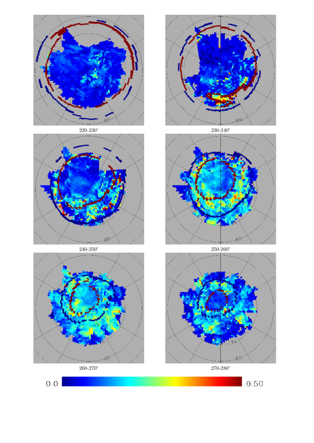
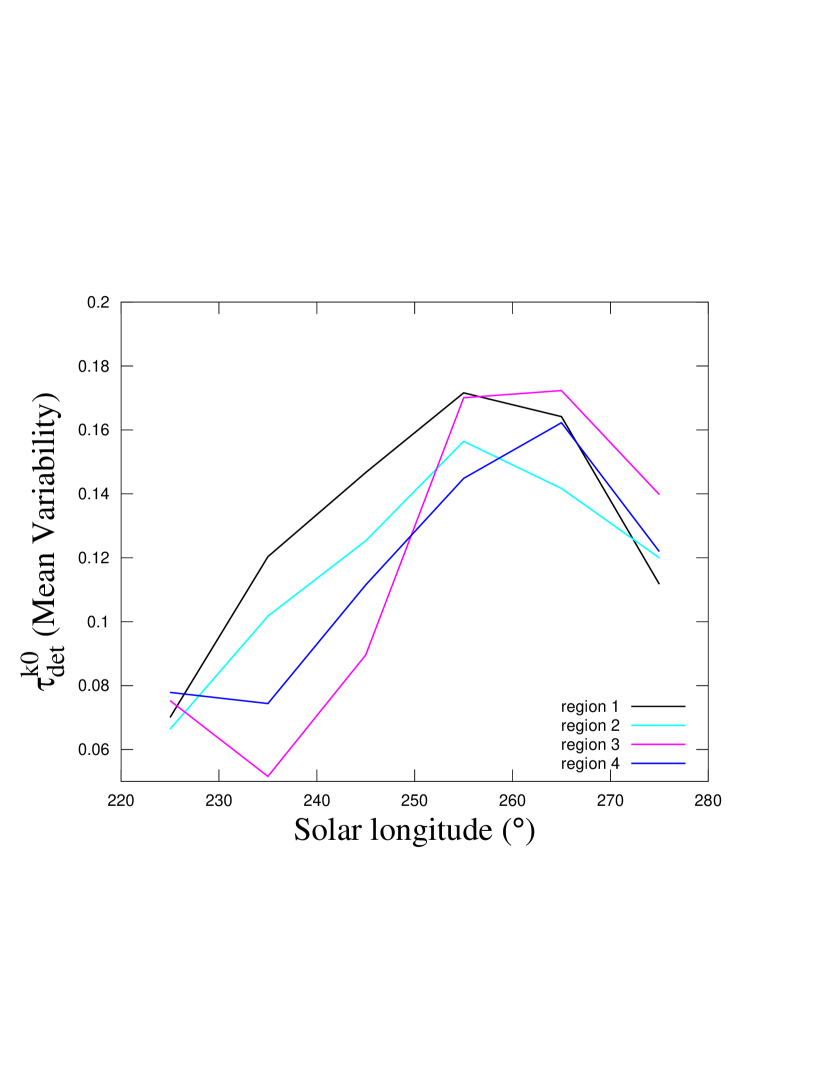 |
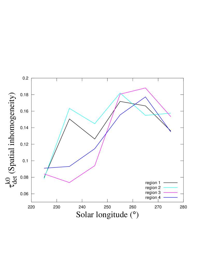 |