Radial evolution of the wave-vector anisotropy of solar wind turbulence between 0.3 and 1 AU

Abstract

We present observations of the power spectral anisotropy in wave-vector space of solar wind turbulence, and study how it evolves in interplanetary space with increasing heliocentric distance. For this purpose we use magnetic field measurements made by the Helios-2 spacecraft at three positions between 0.29 and 0.9 AU. To derive the power spectral density (PSD) in $(k_{\parallel},k_{\bot})$-space based on single-satellite measurements is a challenging task not yet accomplished previously. Here we derive the spectrum $\rm{PSD}_{\rm{2D}}$($\rm{k}_{\parallel}$, $\rm{k}_{\bot}$) from the spatial correlation function $\rm{CF}_{\rm{2D}}(r_{\parallel},r_{\bot})$ by a transformation according to the projection-slice theorem. We find the so constructed PSDs to be distributed in k-space mainly along a ridge that is more inclined toward the $\rm{k}_{\bot}$ than $\rm{k}_{\parallel}$ axis, a new result which probably indicates preferential cascading of turbulent energy along the $\rm{k}_{\bot}$ direction. Furthermore, this ridge of the distribution is found to gradually get closer to the $\rm{k}_{\bot}$ axis, as the outer scale length of the turbulence becomes larger while the solar wind flows further away from the Sun. In the vicinity of the $\rm{k}_{\parallel}$ axis, there appears a minor spectral component that probably corresponds to quasi-parallel Alfvénic fluctuations. Their relative contribution to the total spectral density tends to decrease with radial distance. These findings suggest that solar wind turbulence undergoes an anisotropic cascade transporting most of its magnetic energy towards larger $\rm{k}_{\bot}$, and that the anisotropy in the inertial range is radially developing further at scales that are relatively far from the ever increasing outer scale.

1 Introduction

Solar wind fluctuations are considered as the genuine and prominent example of magnetohydrodynamic (MHD) turbulence (e.g., Tu & Marsch, 1995; Goldstein et al., 1995; Bruno & Carbone, 2005; Marsch, 2006), which is driven by solar activity and naturally occurs in the inhomogeneous interplanetary space. Through in situ measurements made by the Helios 1 and Helios 2 spacecraft, the space plasma physics community has gained abundant knowledge about the radial evolution of solar wind turbulence in the inner heliosphere. Magnetic power spectra of fluctuations at MHD scales were found (Bavassano et al., 1982) to show two separate frequency ranges, whereby the power in the higher-frequency ($\rm{f}>2.5\times 10^{-3}$ Hz in the spacecraft frame) range decays with radial distance (like $\rm{r}^{-4.2}$) faster than that in the lower-frequency ($\rm{f}<2.5\times 10^{-3}$) range (with radial scaling like $\rm{r}^{-3.2}$).

The radial evolution of the lower-frequency magnetic power spectra can be reproduced by the WKB-theory of Alfvén wave propagation (Whang, 1973; Hollweg, 1974), which predicts a similar radial evolution. Whereas the higher-frequency magnetic power spectra, which show a steeper profile (Kolmogrov-like) with its spectral break frequency shifting towards lower values during the radial evolution, were successfully reproduced by Tu’s turbulence model (Tu et al., 1984; Tu, 1988), which took into account (together with the WKB description) the nonlinear interaction between counter-propagating imbalanced Alfvén waves. Moreover, the normalized cross-helicity (Alfvénicity) was shown to decrease with increasing heliocentric distance (Roberts et al., 1987; Marsch & Tu, 1990; Grappin et al., 1990), which to explain was beyond the scope of Tu’s model. To self-consistently describe the radial evolution of turbulent energy, cross-helicity, and Alfvén ratio, substantial theoretical efforts had to be made, which finally resulted in general transport equations (Marsch & Tu, 1989; Tu & Marsch, 1990; Zhou & Matthaeus, 1989) for the related spectra.

In numerical simulations of MHD turbulence, the assumed background magnetic field ($\mathbf{B}_{0}$) was found to cause spatial anisotropy of the turbulent fluctuations along and across the mean field, with the parallel scale generally being larger than the perpendicular scale (e.g., Shebalin et al., 1983; Biskamp & Müller, 2000; Cho et al., 2002). For balanced strong MHD turbulence with vanishing cross-helicity, the anisotropy is predicted to reveal a scaling relation obeying $\rm{k}_{\parallel}\sim\rm{k}_{\bot}^{2/3}$, which was derived in a phenomenological theory (Goldreich & Sridhar, 1995) based on the conjecture of critical balance, i.e. the rough equality between the linear wave-propagation time and nonlinear eddy-interaction time. Numerical simulations further showed that balanced strong turbulence behaves for strong or weak $\mathbf{B}_{0}$ differently in its scaling properties across $\mathbf{B}_{0}$: Iroshnikov-Kraichnan scaling was found for strong $\mathbf{B}_{0}$ and Goldreich-Shridar scaling for weak $\mathbf{B}_{0}$ (Müller et al., 2003). These different scalings are argued to be probably attributed to an increase of dynamic alignment as the cascade proceeds to smaller scale, which may also induce scaling anisotropy in the plane perpendicular to $\mathbf{B}_{0}$ (Boldyrev, 2005).

However, in the solar wind and particular in fast streams one usually observes imbalanced turbulence with outgoing waves dominating over incoming waves. This imbalanced turbulence implies different nonlinear interaction time scales for the oppositely propagating waves, and is more complex than the balanced one. Its physical nature remains a controversial issue, although several theories have been proposed (Lithwick et al., 2007; Beresnyak & Lazarian, 2008; Chandran, 2008; Podesta & Bhattacharjee, 2010).

The spatial anisotropy of solar wind turbulence was studied by means of data analysis employing various tools, such as correlation function (Matthaeus et al., 1990; Dasso et al., 2005; Osman & Horbury, 2007; Németh et al., 2010), structure function (Luo & Wu, 2010; Chen et al., 2010, 2012), power of magnetic components (Bieber et al., 1996), and power law scaling (Horbury et al., 2008; Podesta, 2009; Wicks et al., 2010, 2011). Scaling anisotropy becomes more clearly visible if one uses a scale-dependent local mean magnetic field ($\mathbf{B}_{0,\rm{local}}$) (which was first introduced by Horbury et al. (2008) applying the wavelet technique) instead of a constant global mean magnetic field (Tessein et al., 2009). Some efforts have been also made to reconstruct magnetic PSD in multi-dimensional wave-vector space by means of the k-filtering method (Sahraoui et al., 2010; Narita et al., 2010), which was developed originally to distinguish a limited number of plane waves from multi-position measurements (Pincon & Lefeuvre, 1991). The integrated $\rm{PSD}_{\rm{1D}}(\rm{k}_{\bot})$ with a spectral index $\sim-1.6$ as obtained from k-filtering method seems to resemble the reduced $\rm{PSD}_{\rm{1D}}(\rm{k}_{\bot})$ as derived from the direct wavelet transformation. However, in some cases studied with the k-filtering method, the integrated $\rm{PSD}_{\rm{1D}}(\rm{k}_{\parallel})$ shows a spectral index $\sim-7.0$ (Sahraoui et al., 2010), differing significantly from the reduced $\rm{PSD}_{\rm{1D}}(\rm{k}_{\parallel})$ ($\sim\rm{k}_{\parallel}^{-2}$) as obtained by the wavelet method (Horbury et al., 2008). The reliability of k-filtering method for estimating turbulent power spectra may need further validation, e.g. by applying it to numerically simulated turbulence with known scaling.

Previous studies have revealed the evolution of reduced 1D-PSD in the inner heliosphere, and have presented evidence of wave-vector anisotropy at specific positions [e.g., 1 AU]. However, the turbulence anisotropy pattern at 0.3 AU (the innermost distance reached in-situ so far) and its evolution trend between 0.3 and 1.0 AU has not yet been investigated. To do this is an important task, because it will provide the needed information about the evolution of the energy cascading route in k-space, and reveal possible ways of turbulent energy dissipation required for sustained solar wind heating. This work is dedicated to a study of MHD turbulence anisotropy and will provide new knowledge on its spectral characteristics. The data analysis to achieve these goals is briefly described as follows.

Firstly, we estimate the second-order structure function as a function of $\theta_{\rm{RB}}$ (the angle between the radial direction and the local mean magnetic field vector). Accordingly, the angular distribution of the spatial correlation function is obtained, using the relation between structure function and correlation function. Secondly, we fit the measured structure function with a compound fit function, resembling a power-law dependence at short scale and giving an exponential trend at large scale. The fitted angular correlation function is subsequently derived. Thirdly, under the assumption of a statistically time-stationary state, the relative 2D-PSD in $(\rm{k}_{\parallel},\rm{k}_{\bot})$ space is constructed from the fitted angular distribution of the correlation function, whereby we make use of the projection-slice theorem which is fundamental for image processing in medical tomography (see Bovik (2000) for a detailed review).

2 Analysis method

In this section, we describe the applied methods and the data analysis, which includes: how to derive angular distributions of the structure function $\rm{SF}(\tau,\theta_{\rm{VB}})$ and the correlation function $\rm{CF}(\tau,\theta_{\rm{VB}})$; how to fit $\rm{SF}(\tau,\theta_{\rm{VB}})$ and $\rm{CF}(\tau,\theta_{\rm{VB}})$ appropriately; and how to obtain $\rm{PSD}_{\rm{2D}}(k_{\parallel},k_{\bot})$ as transformed from $\rm{CF}(\tau,\theta_{\rm{VB}})$, which is in turn obtained from $\rm{CF}(r_{\parallel},r_{\bot})$ by assuming a quasi-steady state with $r_{\parallel}\simeq V_{\rm{sw}}\tau\cos\theta_{\rm{VB}}$ and $r_{\bot}\simeq V_{\rm{sw}}\tau\sin\theta_{\rm{VB}}$, corresponding to the Taylor assumption of fluctuations being frozen into the flow, and thus being simply convected by the wind past the spacecraft. Here $V_{\rm{sw}}$ is the solar wind speed.

The second-order magnetic structure function is defined as the ensemble average of the squared magnetic field vector difference. It can be written as

$${\rm{SF}}(\tau)=\left\langle{({\mathbf{B}(t+\frac{\tau}{2})-\mathbf{B}(t-\frac{\tau}{2})})^{2}}\right\rangle,$$ (1)

where the angular bracket denotes in practice a time average in our subsequent data analysis. This time average permits one to quantify the global scaling of the magnetic fluctuations, without distinguishing a possible scaling-law difference for different angles ($\theta_{\rm{VB}}$) between the sampling direction and the local mean magnetic field vector ($\mathbf{B}_{0,\rm{local}}$). The local mean magnetic field is known to be changing in time and depend on scale ($\mathbf{B}_{0,\rm{local}}(t,\tau)$), leading to a scale-dependent variation of the angle $\theta_{\rm{VB}}$ with time. For solar wind with a radial speed much larger than the velocity fluctuation amplitude, the quantity $\theta_{\rm{VB}}$ can be approximated by $\theta_{\rm{RB}}$ (i.e., the angle between the radial direction and the $\mathbf{B}_{0,\rm{local}}$ direction), which is used hereafter. To estimate the structure function value at a certain time scale $\tau^{\prime}$ and for a certain angle $\theta^{\prime}_{\rm{RB}}$, one needs to pick out the values of ${\rm{SF}}(t,\tau^{\prime})$ at those times when $\theta_{\rm{RB}}(t,\tau^{\prime})=\theta^{\prime}_{\rm{RB}}$, and then make an average over all the so picked samples. Therefore, the corresponding angular distribution of the structure function can be expressed as

$${\rm{SF}}(\tau^{\prime},\theta^{\prime}_{\rm{RB}})=\frac{\int_{0}^{T}{(\mathbf{B}(t+\frac{{\tau^{\prime}}}{2})-\mathbf{B}(t-\frac{{\tau^{\prime}}}{2}))^{2}dt\left|{{}_{\theta_{\rm{RB}}(t,\tau^{\prime})=\theta^{\prime}_{\rm{RB}}}}\right.}}{\int_{0}^{T}{dt\left|{{}_{\theta_{\rm{RB}}(t,\tau^{\prime})=\theta^{\prime}_{\rm{RB}}}}\right.}}.$$ (2)

Here the time period for the whole chosen data set is indicated as $T$. It should be much larger than the time scale $\tau^{\prime}$, and thus we may formally take the limit $T\rightarrow\infty$.

Expressing the ensemble average used in equation (1) explicitly as a time average, the relation between the structure function $\rm{SF}(\tau)$ and the correlation function $\rm{CF}(\tau)$ can be obtained from the subsequent calculation:

$$\begin{split}{\rm{SF}}(\tau)&=\frac{1}{T}\int_{0}^{T}(\mathbf{B}(t+\frac{\tau}{2})-\mathbf{B}(t-\frac{\tau}{2}))^{2}dt\\ &=\frac{1}{T}\left[\int_{0}^{T}\mathbf{B}^{2}(t+\frac{\tau}{2})dt+\int_{0}^{T}\mathbf{B}^{2}(t-\frac{\tau}{2})dt-2\int_{0}^{T}\mathbf{B}(t+\frac{\tau}{2})\cdot\mathbf{B}(t-\frac{\tau}{2})dt\right]\\ &=2\rm{CF}(\tau=0)-2\rm{CF}(\tau).\\ \end{split}$$ (3)

Using the above definition (2), the angular distribution of the correlation function can also be approximated by the angular distribution of the structure function, yielding on the basis of (3) the following relation:

$$\begin{split}\rm{SF}(\tau,\theta^{\prime})&=-2\left\langle\mathbf{B}(t+\frac{\tau}{2})\cdot\mathbf{B}(t-\frac{\tau}{2})\right\rangle\left|{{}_{\theta_{RB}=\theta^{\prime}}}\right.+\left\langle\mathbf{B}^{2}(t+\frac{\tau}{2})\right\rangle\left|{{}_{\theta_{RB}=\theta^{\prime}}}\right.+\left\langle\mathbf{B}^{2}(t-\frac{\tau}{2})\right\rangle\left|{{}_{\theta_{RB}=\theta^{\prime}}}\right.\\ &\simeq-2\,\rm{CF}(\tau,\theta^{\prime})+2\,\rm{CF}(\tau=0,\theta^{\prime})\\ &\simeq-2\,\rm{CF}(\tau,\theta^{\prime})+2\,\rm{CF}(\tau=0),\\ \end{split}$$ (4)

where angular isotropy of $\rm{CF}$ at $\tau=0$ was assumed in the derivation. Under Taylor’s hypothesis the solar wind fluctuations can be considered time stationary, as the wave phase speed is small in comparison to the supersonic convection speed, and then $\rm{CF}(\tau,\theta^{\prime})$ can be rewritten as a spatial correlation function in the 2D r-space,

$$\begin{split}\rm{CF}(\tau,\theta^{\prime})\sim\rm{CF}_{\rm{2D}}(r_{\parallel},r_{\bot}),\end{split}$$ (5)

with $r_{\parallel}=V_{\rm{sw}}\tau\cos\theta^{\prime}$ and $r_{\bot}=V_{\rm{sw}}\tau\sin\theta^{\prime}$. This completes the derivation of the two-dimensional correlation function from the structure function. We note that the frozen-in-flow Taylor’s hypothesis may be slightly weakened for smaller heliocentric distance with smaller Alfvén Mach number, which drops from higher than 10 at 1 AU to 3-4 near 0.29 AU. The quantity of main interest is the power spectral density $\rm{PSD}_{\rm{2D}}(k_{\parallel},k_{\bot})$, which in can in principle be obtained directly from Fourier transformation of $\rm{CF}_{\rm{2D}}(r_{\parallel},r_{\bot})$ as follows:

$$\rm{PSD}_{\rm{2D}}(k_{\parallel},k_{\bot})=\int_{-\infty}^{+\infty}{\int_{-\infty}^{+\infty}{\rm{CF}_{\rm{2D}}(r_{\parallel},r_{\bot})\exp(-i(k_{\parallel}r_{\parallel}+k_{\bot}r_{\bot}))dr_{\parallel}dr_{\bot}}}.$$ (6)

However, we take here a new route to estimate $\rm{PSD}_{\rm{2D}}(k_{\parallel},k_{\bot})$. It can also be derived from the projected (integrated) 1D correlation function on the basis of the projection-slice theorem (Bovik, 2000) with help of the following formula:

$$\begin{split}\rm{PSD}_{\rm{2D}}(k,\theta_{k})&=\int_{-\infty}^{+\infty}{\int_{-\infty}^{+\infty}{\rm{CF}_{\rm{2D}}(r_{\parallel},r_{\bot})\exp(-i(k(r_{\parallel}\cos\theta_{k}+r_{\bot}\sin\theta_{k})))dr_{\parallel}dr_{\bot}}}\\ &=\int_{-\infty}^{+\infty}{\int_{-\infty}^{+\infty}{\rm{CF}_{\rm{2D}}(r^{\prime}\cos\theta_{k}-u^{\prime}\sin\theta_{k},r^{\prime}\sin\theta_{k}+u^{\prime}\cos\theta_{k})\exp(-i(kr^{\prime}))dr^{\prime}du^{\prime}}}\\ &=\int_{-\infty}^{+\infty}{\rm{CF}_{\rm{1D}}(r^{\prime};\theta_{k})\exp(-i(kr^{\prime}))dr^{\prime}},\\ \end{split}$$ (7)

where $\theta_{k}$ is the angle between $\mathbf{k}$ and $\mathbf{B}_{0,\rm{local}}$, and $\rm{CF}_{\rm{1D}}(r^{\prime};\theta_{k})$ is the 1D projection (integration) of $\rm{CF}_{\rm{2D}}(r_{\parallel},r_{\bot})$ along the direction normal to $\mathbf{k}$,

$$\rm{CF}_{\rm{1D}}(r^{\prime};\theta_{k})=\int_{-\infty}^{+\infty}{\rm{CF}_{\rm{2D}}(r^{\prime}\cos\theta_{k}-u^{\prime}\sin\theta_{k},r^{\prime}\sin\theta_{k}-u^{\prime}\cos\theta_{k})du^{\prime}}.$$ (8)

Therefore, there are two approaches to calculate $\rm{PSD}_{\rm{2D}}(k_{\parallel},k_{\bot})$, one may adopt either Equation 6 or 7. In practice, the estimation of the 2D correlation function with help of Equation 6 introduces some uncertainty, as the noise involved in the data may destroy the required positivity of the $\rm{PSD}$ in the entire $(k_{\parallel},k_{\bot})$ space. To guarantee this positivity of $\rm{PSD}$ everywhere, one needs to approximate the $\rm{CF}$ with some kind of positive-definite fit function before the Fourier transformation. It is hard to find an adequate function that globally fits the observed $\rm{CF}_{\rm{2D}}(r_{\parallel},r_{\bot})$ well, whereas it is relatively easy to choose a proper fitting function for the projected $\rm{CF}_{\rm{1D}}(r;\theta_{k})$. Therefore, in our work, we will use a fitted $\rm{CF}_{\rm{1D}}(r;\theta_{k})$ to reconstruct reliably the $\rm{PSD}_{\rm{2D}}(k_{\parallel},k_{\bot})$ according to Equation 7.

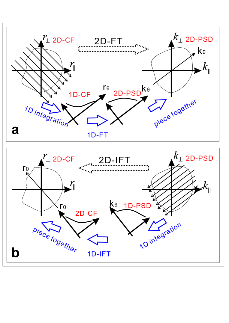
Figure 1: Sketch of relation between 2D-PSD and 2D-CF based on the projection-slice theorem. (Top) Two approaches to derive $\rm{PSD}_{\rm{2D}}(k_{\parallel},k_{\bot})$ from $\rm{CF}_{\rm{2D}}(r_{\parallel},r_{\bot})$: direct 2D Fourier transform and indirect Fourier transform of the projected $\rm{CF}_{\rm{1D}}(r,\theta)$. (Bottom) Vice versa for the derivation of $\rm{CF}_{\rm{2D}}(r_{\parallel},r_{\bot})$ from $\rm{PSD}_{\rm{2D}}(k_{\parallel},k_{\bot})$

To provide the reader with an intuitive impression about the relations between $\rm{CF}_{\rm{2D}}(r_{\parallel},r_{\bot})$, $\rm{CF}_{\rm{1D}}(r,\theta_{k})$, and $\rm{PSD}_{\rm{2D}}(k_{\parallel},k_{\bot})$, we present the schematic illustration shown in the upper panel of Figure 1, which explains the two roads from $\rm{CF}_{\rm{2D}}$ to $\rm{PSD}_{\rm{2D}}$ (direct 2D Fourier transform and indirect method based on the projection-slice theorem). Similarly, one slice of $\rm{CF}_{\rm{2D}}$ at certain angle $\theta_{r}$ is also the 1D inverse Fourier transform of $\rm{PSD}_{\rm{1D}}$ as projected from $\rm{PSD}_{\rm{2D}}$ onto the corresponding direction $\mathbf{k}$ with $\theta_{\rm{kB}}=\theta_{r}$, an approach which is displayed in the lower panel of Figure 1. The relation between $\rm{CF}_{\rm{2D}}$ and $\rm{PSD}_{\rm{1D}}$ is the basic method for calculating $\rm{CF}_{\rm{2D}}$, which was used in previous studies (Matthaeus et al., 1990; Dasso et al., 2005; Osman & Horbury, 2007). In principle, it is also possible to derive $\rm{PSD}_{\rm{2D}}$ from $\rm{PSD}_{\rm{1D}}$ according to the method of inverse Radon transform (filtered back-projection) (private communication with M. Forman). However, this method fails in a typical benchmark test due to extreme large PSD at small $|\mathbf{k}|$, which blurs the entire reconstructed $\rm{PSD}_{\rm{2D}}$ thereby destroying its original pattern.

Speaking of the fitting function for the $\rm{CF}$, we need to mention also the fitting function for the $\rm{SF}$, which is used to reproduce the key features of the $\rm{SF}$. For example, people usually adopt an exponential function to fit the profile of the $\rm{SF}$ at large scale, while they use a power-law function for the small-scale trend. However, as far as we know, there exists no attempt to describe both the small-scale power-law trend and the large-scale exponential trend simultaneously with a single fitting function. To fulfill this task, we suggest a compound function,

$$\rm{SF}(\tau)=2R_{0}\cdot[1-\exp(-(\frac{\tau}{{\tau_{c}}})^{p})],$$ (9)

which interpolates between these limits. There are three parameters to be fitted: $R_{0}$ means the auto-covariance at $\tau=0$, $\tau_{c}$ represents the correlation time at large scale, and the index $p$ describes the power-law scaling at short scale. Generally, for $\rm{SF}(\tau,\theta_{\rm{RB}})$ at different $\theta_{\rm{RB}}$, the parameters $R_{0}$ and $\tau_{c}$ do not change a lot, while $p$ remains variable. Therefore, in our practice, $R_{0}$ and $\tau_{c}$ are obtained by fitting the time-averaged $\rm{SF}(\tau)$, and then $p$ is determined at various $\theta_{\rm{RB}}$ by fitting $\rm{SF}(\tau,\theta_{\rm{RB}})$, but only after $R_{0}$ and $\tau_{c}$ were set. Another practical reason for presetting $R_{0}$ and $\tau_{c}$ before fitting $\rm{SF}(\tau,\theta_{\rm{RB}})$ is that for every $\theta_{\rm{RB}}$ the calculated $\rm{SF}(\tau,\theta_{\rm{RB}})$ is usually unable to reach to the outer scale.

3 Data analysis results

The magnetic data (with a time resolution of about 0.25 s) used here is from measurements by Helios-2 spacecraft at three radial positions (0.29, 0.65, and 0.87 AU) during three time intervals (day of year: 106-109, 76-78, and 49-51 in 1976). The solar wind streams explored during these time intervals are known to be recurrent streams emanating from a common source region on the Sun (Bavassano et al., 1982). The corresponding radial evolution of 1D reduced magnetic PSD was presented in that paper, which observationally promoted the development of the WKB-like solar wind turbulence model (Tu et al., 1984). Three decades later, we analyse the same data set again, but for the purpose of revealing the evolution of solar wind turbulence in terms of its wave-vector anisotropy.

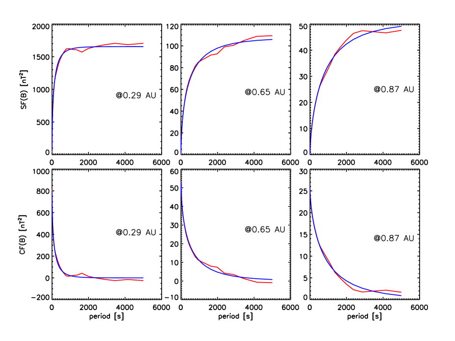
Figure 2: (Top) Time averaged second-order structure functions based on Equation 1 (red) at three positions (0.29, 0.65, and 0.87 AU) and their corresponding fitting results according to Equation 9 (blue). The sets of the three fitting parameters ($R_{0}~{}[\rm{nT}^{2}]$, $t_{c}~{}[s]$, and $p$) are (827, 116, 0.61), (53, 465, 0.61), and (25, 857, 0.67) at 0.29, 0.65, and 0.87 AU. (Bottom) Corresponding correlation functions based on Equation 3 (estimations in red, fitting results in blue).

We use Equation 2 to estimate the second-order structure function $\rm{SF}(\tau)$. It is defined as the magnetic vector difference squared, which is averaged respectively over the three time intervals of our data set. During the estimation, the data gaps are excluded without making any type of interpolation. The top three panels of Figure 2 illustrate the estimation results as red curves. The blue lines are fitting results based on Equation 9, which basically match the estimates at both small and large scales. The fitting parameters ($R_{0}$[$\rm{nT}^{2}$], $t_{c}$[s], $p$) at three radial positions are found to be: (827, 116, 0.61), (53, 465, 0.61), and (25, 857, 0.67), respectively. The fitting parameter $t_{c}$ (corresponding to the correlation time) increases with heliographic distance. The values of the exponent $p$ relate to the power-law index ($\sim-(p+1)$) of the corresponding PSDs, which is found to be around $-1.6$, i.e. near the Kolmogorov value of $-5/3$. The bottom three panels of Figure 2 show the corresponding correlation function $\rm{CF}(\tau)$ as derived from Equation 3.

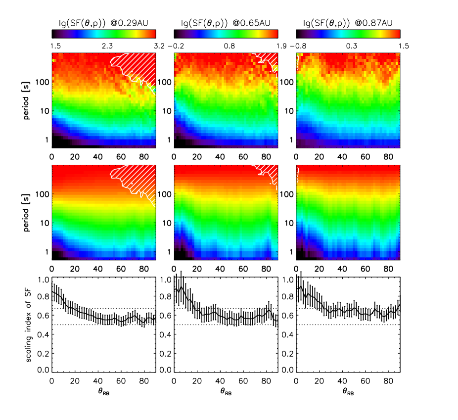
Figure 3: (Top) Angular distribution of second-order structure functions $\rm{SF}(\tau,\theta_{\rm{RB}})$ estimated on the basis of Equation 2. (Middle) Fitting results for $\rm{SF}(\tau,\theta_{\rm{RB}})$ with $\rm{SF}(\tau)$ at every $\theta_{\rm{RB}}$ being fitted according to Equation 9, whereby $p$ is fitted in angular dependence. (Bottom) Fit parameter $p$ as a function of $\theta_{\rm{RB}}$, revealing the scaling anisotropy of the structure function. The error-bars denote the fitting errors of the parameter $p$.

We calculate the structure functions in the angular dimension as a function of $\theta_{\rm{RB}}$ according to Equation 2, and display them in the first row of Figure 3. Apparently, the distribution of $\rm{SF}$ is not uniform in the angle range between $0^{\circ}$ and $90^{\circ}$, with a lower level near $0^{\circ}$. The non-uniform angular distribution is more significant at short scales [e.g., $<100$ s]. For $\rm{SF}(\tau,\theta_{\rm{RB}})$ at larger scales ($\tau>100$ s), it gradually changes from uniformity at 0.29 AU to non-uniformity at 0.87 AU. This angular non-uniformity is a feature hinting at anisotropy of the power spectrum in the wave-vector space. Likewise, the extension of the angular non-uniformity towards larger scales indicates that the wave-vector anisotropy of larger-scale fluctuations evolves as heliocentric distance increases.

We also fit the estimated structure function by the function $\rm{SF}(\tau,\theta_{\rm{RB}})$ of Equation 9. To make sure the fitting process converges for every angle, we restrict the number of fitting parameters to $p$, while we fix the other two parameters ($R_{0}$ and $t_{c}$), both of which may be regarded as constant without angular dependence. The fitted angular distributions are illustrated in the second row of Figure 3, which look similar to the observations. The angular dependence of the fit parameter $p$ is plotted in the third row, showing that the angular variation of $\rm{SF}(\tau,\theta_{\rm{RB}})$ is non-uniform not only in magnitude (first row in Figure 3) but also in the scaling index (third row). We note that $\rm{SF}(\tau,\theta_{\rm{RB}})$ as shown in Figure 3 relates to the squared module of the magnetic-vector difference ($\delta B^{2}_{x}+\delta B^{2}_{y}+\delta B^{2}_{z}$). The structure function $\rm{SF}(\tau,\theta_{\rm{RB}})$ for the component $\delta B^{2}_{\parallel}$ (parallel to $\mathbf{B}_{\rm{0,local}}$) shows a similar non-uniform angular dependence. However, the calculated $\rm{SF}$ for $\delta B^{2}_{\parallel}$ has a plain segment starting at small $\tau$, and cannot be fitted well by the function of Equation 9.

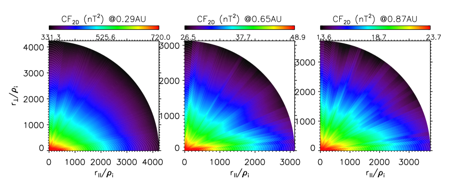
Figure 4: Angular distribution of $\rm{CF}_{\rm{2D}}$ as derived from $\rm{SF}(\tau,\theta_{\rm{RB}})$ according to Equation 4 and displayed in $(r_{\parallel},r_{\bot})$ space under the Taylor hypothesis of near time-stationarity. An elongation of $\rm{CF}$ along $r_{\parallel}$, implying the location of most turbulent energy close to $k_{\bot}$, is revealed at all positions. The proton gyroradius $\rho_{\rm{g}}$ is 17, 48, and 70 km at 0.29, 0.65, and 0.87 AU. It is used for normalization of the spatial coordinates.

The angular distribution of the correlation function $\rm{CF}(\tau,\theta_{\rm{RB}})$ is derived from the fit function $\rm{SF}(\tau,\theta_{\rm{RB}})$ according to Equation 4. In the light of the projection-slice theorem as applied to the relationship between the 2D functions $\rm{CF}$ and $\rm{PSD}$ (lower panel in Figure 1), the quantity $\rm{CF}(\tau,\theta_{\rm{RB}})$ is essentially a 2D correlation function $\rm{CF}(r_{\parallel},r_{\bot})$, which is in principle an inverse Fourier transform of the 2D $\rm{PSD}(k_{\parallel},k_{\bot})$ yet not known. In Figure 4, we plot the resulting $\rm{CF}(r_{\parallel},r_{\bot})$. The coordinates of the abscissa ($r_{\parallel}$) and ordinate ($r_{\bot}$) are estimated by $r_{\parallel}=V_{\rm{sw}}\tau\cos\theta_{\rm{RB}}$ and $r_{\bot}=V_{\rm{sw}}\tau\sin\theta_{\rm{RB}}$, respectively. The main part of $\rm{CF}(r_{\parallel},r_{\bot})$ is elongated along $r_{\parallel}$, which is similar to the “2D” population of the so-called Maltese cross (Matthaeus et al., 1990). However, the “slab” population, which was reported in previous statistical studies of $\rm{CF}$ with $r_{\parallel}$ parallel to the direction of interval-averaged (non-local) magnetic field (Matthaeus et al., 1990; Dasso et al., 2005), is not so prominent in our cases.

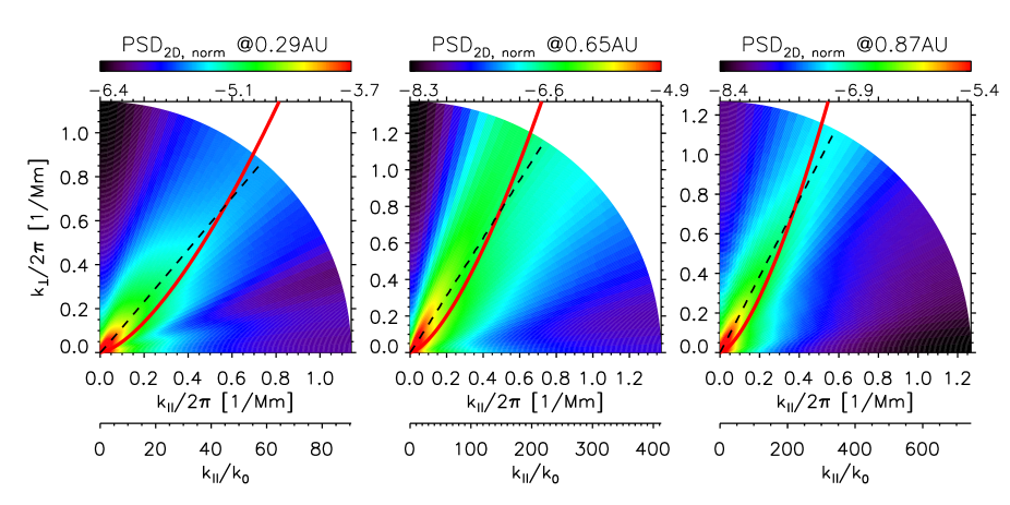
Figure 5: $\rm{PSD}_{\rm{2D}}(k_{\parallel},k_{\bot})$ at three positions (0.29, 0.65, and 0.87 AU) as derived from $\rm{CF}_{\rm{2D}}(r_{\parallel},r_{\bot})$ according to Equation 7 following the projection-slice theorem. The major components (ridge distribution with its centroid position aligned as black dashed line) may be roughly described by Equation 10 shown as red solid line, which means the wave-vector anisotropy develops as the outer-scale wave-number ($k_{0}$) becomes smaller with increasing heliocentric distance. A weakening trend of the minor component that is inclined to $k_{\parallel}$ becomes also visible.

Ideally, the corresponding $\rm{PSD}(k_{\parallel},k_{\bot})$ can be gained directly from 2D Fourier transform of $\rm{CF}_{\rm{2D}}(r_{\parallel},r_{\bot})$. However, in practice, the transformed value might be negative or not certainly positive, thereby restraining the application of the direct 2D Fourier transform. To obtain $\rm{PSD}_{\rm{2D}}(k_{\parallel},k_{\bot})$, we then turn to Equation 7 for a step-by-step derivation. Firstly, by integrating $\rm{CF}_{\rm{2D}}(r_{\parallel},r_{\bot})$ over the path normal to the direction with certain angle $\theta^{\prime}$ with respect to $r_{\parallel}$, the reduced 1D $\rm{CF}_{\rm{1D}}(r)$ corresponding to the angle $\theta^{\prime}$ is calculated. Secondly, the corresponding $\rm{PSD}$ as a Fourier transform of $\rm{CF}_{\rm{1D}}$ is calculated. To guarantee the positivity of the estimated $\rm{PSD}$, $\rm{CF}_{\rm{1D}}$ is fitted before transformation with a function related to that for $\rm{SF}$ as previously described. According to the projection-slice theorem, the estimated $\rm{PSD}$ profile is essentially a slice of $\rm{PSD}_{\rm{2D}}(k_{\parallel},k_{\bot})$ along $\mathbf{k}$ with $\theta^{\prime}$ with respect to $k_{\parallel}$. Thirdly, $\rm{PSD}_{\rm{2D}}(k_{\parallel},k_{\bot})$ is formed by assembling various $\rm{PSD}$ profiles, with different angles ranging from $0^{\circ}$ to $90^{\circ}$ with respect to $k_{\parallel}$. We note that, in calculation, $\rm{CF}_{\rm{2D}}$ and $\rm{CF}_{\rm{1D}}$ one cannot let $r$ go to infinity. As a result, the transformed $\rm{PSD}_{\rm{2D}}$ may slightly depart from the real one. Therefore, in Figure 5, we just present the normalized $\rm{PSD}_{\rm{2D,n}}$ rather than the absolute $\rm{PSD}_{\rm{2D}}$. The uncertainty (confidence interval) for the estimated $\rm{PSD}_{\rm{2D}}$ is not provided here, since due to the complexity of the estimation method that was not yet possible.

Obviously, the normalized $\rm{PSD}_{\rm{2D,n}}$ shown in Figure 5 is not uniformly distributed at all angles, indicating an anisotropic wave-vector distribution. This anisotropy is mainly characterized by a ridge distribution which has a bias towards $k_{\bot}$ as compared to $k_{\parallel}$. Moreover, as the heliographic distance increases, the ridge distribution becomes more inclined toward $k_{\bot}$ at the same $|k|$, in association with lower PSD (darker blue in the figure) around the $k_{\parallel}$ region and higher PSD (brighter blue in the figure) around the $k_{\bot}$ region. The discovery of this bent ridge and its radial evolution imply that solar wind turbulent energy cascades preferentially along the $k_{\bot}$ as compared to the $k_{\parallel}$ axis, and the turbulence cascade radially develops with more energy cascading to the $k_{\bot}$ region, as the scale ($1/|k|$) is shifting away from the radially-growing outer scale ($1/|k_{0}|$). In addition to the major ridge distribution, a minor population seems to exist close to $k_{\parallel}$ (see Figure 5a), and appears to become weaker at farther distances (see Figures 5b,c). The observational fact that $\rm{PSD}$ is composed of two populations, with the major one bending more perpendicularly and the minor one becoming weaker, seems compatible with the previously suggested two-component turbulence model, which invokes non-damping convective structures (spatially varying across $\mathbf{B}_{0}$) that are superposed on damping Alfvén waves (spatially varying along $\mathbf{B}_{0}$) (Tu & Marsch, 1993).

To emphasize the trend of the ridge distribution and its radial evolution, we estimate the ridge position of every scale by averaging the angles with local lg(PSD) as the weights (i.e., first-order moment centroid method). The estimated ridge positions are shown as black dashed lines in Figure 5 and appear straight. Whether or not the straightness is realistic is yet unknown. Furthermore, we fit the estimated ridge position with following simple formula,

$$k_{\parallel}=\alpha\cdot k_{0}^{1/3}\cdot k_{\bot}^{2/3},$$ (10)

where $k_{0}(=2\pi/(V_{\rm{sw}}\cdot\tau_{c}))$ is related to the outer-scale wave-number. $\alpha$ is the coefficient to be fitted, which is $\sim$ 3.2, 3.9, and 3.9 for our three cases. We find that the simple $k_{\parallel}\rm{-}k_{\bot}$-relation profile according to Equation 10 is basically coincident with the observed ridge distribution. However, some departures, e.g., the estimated black dashed line looks more straight than the fitted red line, still remain. Nevertheless, the relation ($k_{\parallel}\sim k_{0}^{1/3}k_{\bot}^{2/3}$), as predicted by the critical-balance hypothesis (Goldreich & Sridhar, 1995) for MHD turbulence, seems to describe well the observed anisotropy of solar wind turbulence. The role of $k_{0}$, which was once neglected in previous observational studies, in shaping the anisotropy shall be emphasized here. It may be the reduction in $k_{0}$ which causes the development of the spectral anisotropy (increasing inclination toward $k_{\bot}$ at the same $|k|$) in interplanetary space as heliographic distance increases.

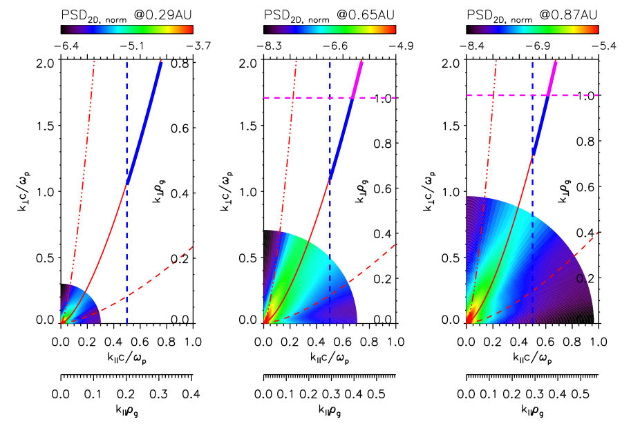
Figure 6: Implication of solar wind heating mechanism from the extension of ridge profile. Red solid lines denote the extended ridge profiles ($k_{\parallel}=\alpha\cdot k_{0}^{1/3}\cdot k_{\bot}^{2/3}$ with $\alpha=3.2,3.9,3.9$ for the three panels) as superposed on $\rm{PSD}_{\rm{2D}}(k_{\parallel},k_{\bot})$ in larger wave-vector space. Large $k_{\parallel}$ with $k_{\parallel}c/\omega_{\rm{p}}>0.5$ (to the right of blue dashed line) indicates the region of ion cyclotron resonance. Landau resonance becomes active when $k_{\bot}\rho_{\rm{g}}>1$ (above magenta dashed line) and dominant for $k_{\parallel}c/\omega_{\rm{p}}\ll 1.0$. Radial evolution of the approximated ridge profile and its intersections with the threshold lines ($k_{\parallel}c/\omega_{\rm{p}}=0.5$ and $k_{\bot}\rho_{\rm{g}}=1$) indicate the transition of cascade termination from cyclotron resonance to Landau resonance as the solar wind flows further away. Ridge profiles with larger (smaller) $\alpha(=10(1.1))$ (red dashed (red dash-dot-dot) lines) would lead to cyclotron resonance (Landau resonance) separately at all distances without a transition, which seems unrealistic. The proton gyroradius (proton inertial length) $\rho_{\rm{g}}(c/\omega_{\rm{p}})$ is 17(42), 48(82), and 70(121) km at 0.29, 0.65, and 0.87 AU.

Solar wind heating mechanism may be inferred from the radial evolution of the ridge trend. According to linear Vlasov theory, Alfvén waves with plasma $\beta_{\rm{p}}\in[0.1,1.0]$ usually become dissipated due to proton cyclotron resonance when they have $k_{\parallel}c/\omega_{\rm{p}}\in[0.1,1.0]$, where $c/\omega_{\rm{p}}$ is the proton inertial length (Gary & Nishimura, 2004). On the other hand, Landau resonance becomes more and more prominent as plasma $\beta_{p}$ rises (Gary & Nishimura, 2004) and $k_{\bot}\rho_{\rm{g}}$ increases (Howes et al., 2006), where $\rho_{\rm{g}}$ is the proton gyroradius. Howes (2011) pointed out that, Landau damping calculated in the gyro-kinetic limit is not sufficient for the empirically estimated proton heating (Cranmer et al., 2009) at small heliocentric distances ($R<0.8$ AU). At these small distances, turbulent cascade is speculated to approach to proton cyclotron frequency before being terminated by Landau resonance (Howes, 2011). However, the relative contributions from cyclotron resonance and Landau resonance to solar wind heating at different radial distances have not yet been addressed from observations. The approximated relation ($k_{\parallel}=\alpha\cdot k_{0}^{1/3}\cdot k_{\bot}^{2/3}$ with $\alpha\in[3,4]$) for the observed ridge distribution may be used to address this issue. In Figure 6, we just simply extend the approximated ridge profile in a larger wave-vector space to see what kind of resonance (cyclotron or Landau) would probably terminate the cascade. As a result, we find that, at the three distances within 1 AU, the extended ridge profile clearly approaches to cyclotron resonance (marked by $k_{\parallel}c/\omega_{\rm{p}}>0.5$) ahead of Landau resonance (marked by $k_{\bot}\rho_{\rm{g}}>1.0$). Moreover, one may expect that, as the distance increases ($\geq 1$ AU) in association with reduction of $k_{0}$, the ridge profile would first exceed the threshold $k_{\bot}\rho_{\rm{g}}=1$ before approaching to $k_{\parallel}c/\omega_{p}=0.5$, which implies a dominance of Landau damping over cyclotron damping at larger distances. According to critical-balance theory in MHD and kinetic regimes(Schekochihin et al., 2009), the extension of ridge in the MHD inertial range may be still related to Equation 10, while the extension part in the kinetic (dissipation) range may deviate from Equation 10 with more inclination towards $k_{\bot}$. For sake of simplicity, we neglect such deviation of extended ridge in the kinetic range from that in the inertial range.

The value of coefficient $\alpha$ is also worth emphasizing here. If $\alpha$ were one third of the approximated value ($3.3/3=1.1$), the ridge profile (red dash-dot-dot line in Figure 6) would exceed $k_{\bot}\rho_{\rm{g}}=1$ without approaching to $k_{\parallel}c/\omega_{\rm{p}}=0.5$, leading to insufficient heating rate by Landau resonance within 1 AU according to the gyro-kinetic prescription by Howes (2011). On the other side, if $\alpha$ were too large (saying $3.3\times 3=10$), the ridge profile (red dashed line in Figure 6) would lie well below $k_{\bot}\rho_{g}=1$, implying the absence of transition from cyclotron damping to Landau damping around 1 AU (inconsistent with the conclusion by Howes (2011)). Therefore, the $\alpha$ value ($\in[3,4]$ obtained here) besides $k_{0}$ is another important parameter for grasping the essence of solar wind heating mechanism. $\alpha$ may be expressed as the ratio of $\varepsilon$ to $V_{\rm{A}}^{3}k_{\rm{0}}$ with $\varepsilon$ being the energy cascade rate if $k_{\parallel}=(\varepsilon/V_{\rm{A}}^{3})^{1/3}k_{\bot}^{2/3}$, which is usually assumed in critical-balance theory (Goldreich & Sridhar, 1995; Schekochihin et al., 2009).

4 Summary and discussion

We have made the first successful attempt to reconstruct, on the basis of single spacecraft measurements, the 2D spectral density $\rm{PSD}_{\rm{2D}}(k_{\parallel},k_{\bot})$ for solar wind MHD turbulence. We estimate the angular distribution of the second-order structure function $\rm{SF}(\tau,\theta_{\rm{RB}})$, and derive the corresponding correlation function $\rm{CF}_{\rm{2D}}(r_{\parallel},r_{\bot})$, which in principle is an inverse 2D Fourier transform of $\rm{PSD}_{\rm{2D}}(k_{\parallel},k_{\bot})$. The transformation from time scale $\tau$ to spatial scale $r$, when building up $\rm{CF}_{\rm{2D}}(r_{\parallel},r_{\bot})$, is based on Taylor’s hypothesis that solar wind fluctuations are quasi-stationary within the flow transit time scale, as the solar wind passes by the spacecraft. The 2D direct Fourier transform of $\rm{CF}_{\rm{2D}}(r_{\parallel},r_{\bot})$ fails to guarantee the required positivity of $\rm{PSD}_{\rm{2D}}(k_{\parallel},k_{\bot})$. Alternatively, we employ for the first time a method based on the projection-slice theorem, which connects the integrated $\rm{CF}_{\rm{1D}}(r,\theta^{\prime})$ with the corresponding slice $\rm{PSD}_{\rm{2D}}(k,\theta^{\prime})$ of the $\rm{PSD}$ via a 1D Fourier transform, to fulfill that task. Before the 1D Fourier transformation, $\rm{CF}_{\rm{1D}}(r,\theta^{\prime})$ is fitted smoothly to guarantee the positivity of the transformed $\rm{PSD}_{\rm{2D}}(k,\theta^{\prime})$.

As a result, $\rm{SF}(\tau,\theta_{\rm{RB}})$ shows a non-uniform angular distribution with more power being located in the perpendicular region ($\theta_{\rm{RB}}\sim 90^{\circ}$) than in the parallel region ($\theta_{\rm{RB}}\sim 0^{\circ}$) of wave-vector space. Moreover, there is angular dependence of the scaling law for $\rm{SF}(\tau,\theta_{\rm{RB}})$ at short scales, whereby the scaling index $p$ drops from $\sim 0.9$ at $\theta_{\rm{RB}}=0^{\circ}$ to $\sim 0.6$ at $\theta_{\rm{RB}}=90^{\circ}$. We find that $\rm{SF}(\tau,\theta_{\rm{RB}})$ have at all three positions (0.29, 0.65, and 0.87 AU) the two above properties, indicating the prevalence of anisotropy in the turbulence throughout the inner heliosphere. This result obtained within 1 AU is similar to that found for the $\rm{SF}$ anisotropy beyond 1 AU (Luo & Wu, 2010). The corresponding correlation functions $\rm{CF}_{\rm{2D}}(r_{\parallel},r_{\bot})$ clearly show that magnetic fluctuations are correlated at longer (shorter) length along (across) the background magnetic field.

The corresponding $\rm{PSD}_{\rm{2D}}(k_{\parallel},k_{\bot})$ at the positions within 1 AU is revealed to have a ridge distribution with a bias towards $k_{\bot}$ as compared to $k_{\parallel}$, suggesting a preferential cascading along $k_{\bot}$. This kind of ridge distribution has never been reported in previous studies at 1 AU, e.g. those based on the wave-telescope (k-filtering) method (Narita et al., 2010; Sahraoui et al., 2010). Furthermore, this ridge distribution is found to become ever more inclined toward the $k_{\bot}$ axis with increasing heliographic distance, thus indicating a radial development of the wave-vector anisotropy. The observed radial evolution of the ridge casts new light on the scaling relation between $k_{\parallel}$ and $k_{\bot}$, which may empirically be approximated by $k_{\parallel}\simeq\alpha k_{0}^{1/3}k_{\bot}^{2/3}$, with $\alpha\in[3,4]$ and $k_{0}$ being the wave-number of the outer scale. This approximation for the wave-vector anisotropy seems to indicate critical-balance-type cascading (Goldreich & Sridhar, 1995) of solar wind turbulence. A possible influence of $k_{0}$ on the anisotropy development, which was neglected in previous observational analyses, is also found.

However, the evolution of the ridge distribution cannot represent the whole story about wave-vector anisotropy of solar wind turbulence. There seems to be a minor population located near $k_{\parallel}$, which is beyond the scope of critical-balance turbulence theory. The apparent two-component distribution of $\rm{PSD}_{\rm{2D}}(k_{\parallel},k_{\bot})$ seems to be connected with previous two-component models, e.g., models with “slab”+“2D” (Matthaeus et al., 1990), models composed of Alfvén waves and convected structures (Tu & Marsch, 1993), and conjectures with critical-balanced component plus slab component (Forman et al., 2011; He et al., 2012b). We find that the minor population seems to weaken further with increasing heliographic distance, leaving more energy distributed in the region close to the $k_{\bot}$ axis. This gradual migration of energy towards $k_{\bot}$ might indicate a relative enrichment of turbulence energy carried by convective structures and explain the observed associated shortage of Alfvénicity, which was already discussed in the previous two-component model by Tu & Marsch (1993). The observed “slab”-like minor component is crucial for scattering of energetic particles in the interplanetary space (Bieber et al., 1996; Chandran, 2000; Qin et al., 2002). The radial evolution of anisotropic turbulence may be quantified in the future and incorporated into the transport model of energetic particles.

The estimated $\rm{PSD}_{\rm{2D}}(k_{\parallel},k_{\bot})$ is believed to impose valuable observational constraints on the theoretical models of solar wind turbulence. Recently, Cranmer & van Ballegooijen (2012) modelled $\rm{PSD}_{\rm{2D}}(k_{\parallel},k_{\bot})$ at different heliocentric distances by solving a set of 2D cascade-advection-diffusion equations, with the total power pre-determined by the damped wave-action conservation equation and the reduced $\rm{PSD}_{\rm{1D}}(k_{\bot})$ pre-set by the 1D advection-diffusion equation. Their modelled $\rm{PSD}_{\rm{2D}}(k_{\parallel},k_{\bot})$ looks partly similar to our observational spectrum, in the sense of where the major power is located. However, the differences in distribution pattern and radial evolution between observational and modelled spectra call for a substantial improvement of the models for solar wind turbulence.

The approximated ridge profile as extended to large $k_{\parallel}$ and $k_{\bot}$ may give a hint about the resonance type responsible for solar wind heating at different radial distances. The extended ridge profile at small distances ($R<0.8$ AU) is found to reach larger $k_{\parallel}$ where proton cyclotron resonance acts before Landau damping sets in. As the distance increases, the extended ridge profile, which is inclined more towards $k_{\bot}$ due to the reduction of $k_{0}$, tends to arrive at Landau resonance before cyclotron resonance. Such performance of the approximated ridge profile confirms observationally previous conjecture about the transition from cyclotron resonance to Landau resonance with increasing heliographic distance (Howes, 2011).

Our results are just limited to the MHD inertial range, but the analysis should be extended to kinetic scales where several typical properties have been revealed: steeper power-law magnetic spectrum (Sahraoui et al., 2009; Alexandrova et al., 2009), enhanced electric-field spectrum (Bale et al., 2005), enhanced magnetic compressibility (Smith et al., 2006; Hamilton et al., 2008; Salem et al., 2012; He et al., 2012a), and two-component pattern in the magnetic helicity (He et al., 2011; Podesta & Gary, 2011; He et al., 2012a, b). These observations seem to be in favour of the oblique Alfvén waves or kinetic Alfvén waves (KAW) as the candidate for explaining the dominant fluctuations in ion-scale turbulence. The oblique Alfvén/ion-cyclotron waves may be via resonance diffusion (Marsch & Bourouaine, 2011) responsible for the formation of the observed wide proton beam. The theory of KAW itself and its role in kinetic turbulence have been studied intensively (Hollweg, 1999; Wu & Chao, 2004; Howes et al., 2008; Zhao et al., 2011; Voitenko & de Keyser, 2011; Howes et al., 2011). Ion cyclotron waves, which are considered responsible for the ion perpendicular heating (Bourouaine et al., 2010), were also identified (Jian et al., 2009; He et al., 2011). There are other possible wave modes, e.g. fast whistler waves, ion Bernstein waves, and fast-cyclotron waves, which may exist in kinetic turbulence (Gary et al., 2012; TenBarge et al., 2012; Xiong & Li, 2012). Spectral break at the ion-kinetic scale seems to be almost constant (about 0.5 Hz in the spacecraft frame) with radial distance (Perri et al., 2010; Bourouaine et al., 2012). The spectral break frequency might corresponds to the proton inertial length in quasi-2D turbulence when considering a large-scale background magnetic field $\mathbf{B}_{0}$ (which is obtained through averaging over a time period higher than 1 hour) (Bourouaine et al., 2012). However, not much is presently known about the radial evolution of solar wind turbulence at ion-kinetic scales.

In the future, with the help of high-time-resolution measurements to be made by the wave and particle instruments flown on such mission like Solar Orbiter and Solar Probe Plus, the radial evolution of the wave-vector anisotropy at kinetic scale may be studied, and more new results will be obtained on the spectrum anisotropy in the inertial range that was analysed here.

References

- Alexandrova et al. (2009) Alexandrova, O., Saur, J., Lacombe, C., Mangeney, A., Mitchell, J., Schwartz, S. J., & Robert, P. 2009, Physical Review Letters, 103, 165003
- Bale et al. (2005) Bale, S. D., Kellogg, P. J., Mozer, F. S., Horbury, T. S., & Reme, H. 2005, Physical Review Letters, 94, 215002
- Bavassano et al. (1982) Bavassano, B., Dobrowolny, M., Mariani, F., & Ness, N. F. 1982, J. Geophys. Res., 87, 3617
- Beresnyak & Lazarian (2008) Beresnyak, A., & Lazarian, A. 2008, ApJ, 682, 1070
- Bieber et al. (1996) Bieber, J. W., Wanner, W., & Matthaeus, W. H. 1996, J. Geophys. Res., 101, 2511
- Biskamp & Müller (2000) Biskamp, D., & Müller, W.-C. 2000, Physics of Plasmas, 7, 4889
- Boldyrev (2005) Boldyrev, S. 2005, ApJ, 626, L37
- Bourouaine et al. (2012) Bourouaine, S., Alexandrova, O., Marsch, E., & Maksimovic, M. 2012, ApJ, 749, 102
- Bourouaine et al. (2010) Bourouaine, S., Marsch, E., & Neubauer, F. M. 2010, Geophys. Res. Lett., 37, 14104
- Bovik (2000) Bovik, A. C. 2000, Handbook of Image and Video Processing, ed. Bovik, A. C.
- Bruno & Carbone (2005) Bruno, R., & Carbone, V. 2005, Living Reviews in Solar Physics, 2, 4
- Chandran (2000) Chandran, B. D. G. 2000, ApJ, 529, 513
- Chandran (2008) —. 2008, ApJ, 685, 646
- Chen et al. (2010) Chen, C. H. K., Horbury, T. S., Schekochihin, A. A., Wicks, R. T., Alexandrova, O., & Mitchell, J. 2010, Physical Review Letters, 104, 255002
- Chen et al. (2012) Chen, C. H. K., Mallet, A., Schekochihin, A. A., Horbury, T. S., Wicks, R. T., & Bale, S. D. 2012, ApJ, 758, 120
- Cho et al. (2002) Cho, J., Lazarian, A., & Vishniac, E. T. 2002, ApJ, 564, 291
- Cranmer et al. (2009) Cranmer, S. R., Matthaeus, W. H., Breech, B. A., & Kasper, J. C. 2009, ApJ, 702, 1604
- Cranmer & van Ballegooijen (2012) Cranmer, S. R., & van Ballegooijen, A. A. 2012, ApJ, 754, 92
- Dasso et al. (2005) Dasso, S., Milano, L. J., Matthaeus, W. H., & Smith, C. W. 2005, ApJ, 635, L181
- Forman et al. (2011) Forman, M. A., Wicks, R. T., & Horbury, T. S. 2011, ApJ, 733, 76
- Gary et al. (2012) Gary, S. P., Chang, O., & Wang, J. 2012, ApJ, 755, 142
- Gary & Nishimura (2004) Gary, S. P., & Nishimura, K. 2004, Journal of Geophysical Research (Space Physics), 109, 2109
- Goldreich & Sridhar (1995) Goldreich, P., & Sridhar, S. 1995, ApJ, 438, 763
- Goldstein et al. (1995) Goldstein, M. L., Roberts, D. A., & Matthaeus, W. H. 1995, Ann. Rev. Astron. & Astrophys., 33, 283
- Grappin et al. (1990) Grappin, R., Mangeney, A., & Marsch, E. 1990, J. Geophys. Res., 95, 8197
- Hamilton et al. (2008) Hamilton, K., Smith, C. W., Vasquez, B. J., & Leamon, R. J. 2008, Journal of Geophysical Research (Space Physics), 113, 1106
- He et al. (2011) He, J., Marsch, E., Tu, C., Yao, S., & Tian, H. 2011, ApJ, 731, 85
- He et al. (2012a) He, J., Tu, C., Marsch, E., & Yao, S. 2012a, ApJ, 745, L8
- He et al. (2012b) —. 2012b, ApJ, 749, 86
- Hollweg (1974) Hollweg, J. V. 1974, J. Geophys. Res., 79, 1539
- Hollweg (1999) —. 1999, J. Geophys. Res., 104, 14811
- Horbury et al. (2008) Horbury, T. S., Forman, M., & Oughton, S. 2008, Physical Review Letters, 101, 175005
- Howes (2011) Howes, G. G. 2011, ApJ, 738, 40
- Howes et al. (2006) Howes, G. G., Cowley, S. C., Dorland, W., Hammett, G. W., Quataert, E., & Schekochihin, A. A. 2006, ApJ, 651, 590
- Howes et al. (2008) —. 2008, Journal of Geophysical Research (Space Physics), 113, 5103
- Howes et al. (2011) Howes, G. G., Tenbarge, J. M., Dorland, W., Quataert, E., Schekochihin, A. A., Numata, R., & Tatsuno, T. 2011, Physical Review Letters, 107, 035004
- Jian et al. (2009) Jian, L. K., Russell, C. T., Luhmann, J. G., Strangeway, R. J., Leisner, J. S., & Galvin, A. B. 2009, ApJ, 701, L105
- Lithwick et al. (2007) Lithwick, Y., Goldreich, P., & Sridhar, S. 2007, ApJ, 655, 269
- Luo & Wu (2010) Luo, Q. Y., & Wu, D. J. 2010, ApJ, 714, L138
- Marsch (2006) Marsch, E. 2006, Living Reviews in Solar Physics, 3, 1
- Marsch & Bourouaine (2011) Marsch, E., & Bourouaine, S. 2011, Annales Geophysicae, 29, 2089
- Marsch & Tu (1989) Marsch, E., & Tu, C.-Y. 1989, Journal of Plasma Physics, 41, 479
- Marsch & Tu (1990) —. 1990, J. Geophys. Res., 95, 8211
- Matthaeus et al. (1990) Matthaeus, W. H., Goldstein, M. L., & Roberts, D. A. 1990, J. Geophys. Res., 95, 20673
- Müller et al. (2003) Müller, W.-C., Biskamp, D., & Grappin, R. 2003, Phys. Rev. E, 67, 066302
- Narita et al. (2010) Narita, Y., Glassmeier, K.-H., Sahraoui, F., & Goldstein, M. L. 2010, Physical Review Letters, 104, 171101
- Németh et al. (2010) Németh, Z., Facskó, G., & Lucek, E. A. 2010, Sol. Phys., 266, 149
- Osman & Horbury (2007) Osman, K. T., & Horbury, T. S. 2007, ApJ, 654, L103
- Perri et al. (2010) Perri, S., Carbone, V., & Veltri, P. 2010, ApJ, 725, L52
- Pincon & Lefeuvre (1991) Pincon, J. L., & Lefeuvre, F. 1991, J. Geophys. Res., 96, 1789
- Podesta (2009) Podesta, J. J. 2009, ApJ, 698, 986
- Podesta & Bhattacharjee (2010) Podesta, J. J., & Bhattacharjee, A. 2010, ApJ, 718, 1151
- Podesta & Gary (2011) Podesta, J. J., & Gary, S. P. 2011, ApJ, 734, 15
- Qin et al. (2002) Qin, G., Matthaeus, W. H., & Bieber, J. W. 2002, ApJ, 578, L117
- Roberts et al. (1987) Roberts, D. A., Goldstein, M. L., Klein, L. W., & Matthaeus, W. H. 1987, J. Geophys. Res., 92, 12023
- Sahraoui et al. (2010) Sahraoui, F., Goldstein, M. L., Belmont, G., Canu, P., & Rezeau, L. 2010, Physical Review Letters, 105, 131101
- Sahraoui et al. (2009) Sahraoui, F., Goldstein, M. L., Robert, P., & Khotyaintsev, Y. V. 2009, Physical Review Letters, 102, 231102
- Salem et al. (2012) Salem, C. S., Howes, G. G., Sundkvist, D., Bale, S. D., Chaston, C. C., Chen, C. H. K., & Mozer, F. S. 2012, ApJ, 745, L9
- Schekochihin et al. (2009) Schekochihin, A. A., Cowley, S. C., Dorland, W., Hammett, G. W., Howes, G. G., Quataert, E., & Tatsuno, T. 2009, ApJS, 182, 310
- Shebalin et al. (1983) Shebalin, J. V., Matthaeus, W. H., & Montgomery, D. 1983, Journal of Plasma Physics, 29, 525
- Smith et al. (2006) Smith, C. W., Hamilton, K., Vasquez, B. J., & Leamon, R. J. 2006, ApJ, 645, L85
- TenBarge et al. (2012) TenBarge, J. M., Podesta, J. J., Klein, K. G., & Howes, G. G. 2012, ApJ, 753, 107
- Tessein et al. (2009) Tessein, J. A., Smith, C. W., MacBride, B. T., Matthaeus, W. H., Forman, M. A., & Borovsky, J. E. 2009, ApJ, 692, 684
- Tu & Marsch (1995) Tu, C., & Marsch, E. 1995, Space Science Reviews, 73, 1
- Tu (1988) Tu, C.-Y. 1988, J. Geophys. Res., 93, 7
- Tu & Marsch (1990) Tu, C.-Y., & Marsch, E. 1990, Journal of Plasma Physics, 44, 103
- Tu & Marsch (1993) —. 1993, J. Geophys. Res., 98, 1257
- Tu et al. (1984) Tu, C.-Y., Pu, Z.-Y., & Wei, F.-S. 1984, J. Geophys. Res., 89, 9695
- Voitenko & de Keyser (2011) Voitenko, Y., & de Keyser, J. 2011, Nonlinear Processes in Geophysics, 18, 587
- Whang (1973) Whang, Y. C. 1973, J. Geophys. Res., 78, 7221
- Wicks et al. (2010) Wicks, R. T., Horbury, T. S., Chen, C. H. K., & Schekochihin, A. A. 2010, MNRAS, 407, L31
- Wicks et al. (2011) —. 2011, Physical Review Letters, 106, 045001
- Wu & Chao (2004) Wu, D. J., & Chao, J. K. 2004, Nonlinear Processes in Geophysics, 11, 631
- Xiong & Li (2012) Xiong, M., & Li, X. 2012, Sol. Phys., 279, 231
- Zhao et al. (2011) Zhao, J. S., Wu, D. J., & Lu, J. Y. 2011, Physics of Plasmas, 18, 032903
- Zhou & Matthaeus (1989) Zhou, Y., & Matthaeus, W. H. 1989, Geophys. Res. Lett., 16, 755