Breaking the coherence barrier: A new theory for
compressed sensing

1 Introduction

This paper provides an extension of compressed sensing which bridges a substantial gap between existing theory and its current use in real-world applications.

Compressed sensing (CS), introduced by Candès, Romberg & Tao [14] and Donoho [25], has been one of the major developments in applied mathematics in the last decade [10, 27, 26, 22, 28, 29, 30]. Subject to appropriate conditions, it allows one to circumvent the traditional barriers of sampling theory (e.g. the Nyquist rate), and thereby recover signals from far fewer measurements than is classically considered possible. This has important implications in many practical applications, and for this reason CS has, and continues to be, very intensively researched.

The theory of CS is based on three fundamental concepts: sparsity, incoherence and uniform random subsampling. Whilst there are examples where these apply, in many applications one or more of these principles may be lacking. This includes virtually all of medical imaging – Magnetic Resonance Imaging (MRI), Computerized Tomography (CT) and other versions of tomography such as Thermoacoustic, Photoacoustic or Electrical Impedance Tomography – most of electron microscopy, as well as seismic tomography, fluorescence microscopy, Hadamard spectroscopy and radio interferometry. In many of these problems, it is the principle of incoherence that is lacking, rendering the standard theory inapplicable. Despite this issue, compressed sensing has been, and continues to be, used with great success in many of these areas. Yet, to do so it is typically implemented with sampling patterns that differ substantially from the uniform subsampling strategies suggested by the theory. In fact, in many cases uniform random subsampling yields highly suboptimal numerical results.

The standard mathematical theory of CS has now reached a mature state. However, as this discussion attests, there is a substantial, and arguably widening gap between the theoretical and applied sides of the field. New developments and sampling strategies are increasingly based on empirical evidence lacking mathematical justification. Furthermore, in the above applications one also witnesses a number of intriguing phenomena that are not explained by the standard theory. For example, in such problems, the optimal sampling strategy depends not just on the overall sparsity of the signal, but also on its structure, as will be documented thoroughly in this paper. This phenomenon is in direct contradiction with the usual sparsity-based theory of CS. Theorems that explain this observation – i.e. that reflect how the optimal subsampling strategy depends on the structure of the signal – do not currently exist.

The purpose of this paper is to provide a bridge across this divide. It does so by generalizing the three traditional pillars of CS to three new concepts: asymptotic sparsity, asymptotic incoherence and multilevel random subsampling. This new theory shows that CS is also possible, and reveals several advantages, under these substantially more general conditions. Critically, it also addresses the important issue raised above: the dependence of the subsampling strategy on the structure of the signal.

The importance of this generalization is threefold. First, as will be explained, real-world inverse problems are typically not incoherent and sparse, but asymptotically incoherent and asymptotically sparse. This paper provides the first comprehensive mathematical explanation for a range of empirical usages of CS in applications such as those listed above. Second, in showing that incoherence is not a requirement for CS, but instead that asymptotic incoherence suffices, the new theory offers markedly greater flexibility in the design of sensing mechanisms. In the future, sensors need only satisfy this significantly more relaxed condition. Third, by using asymptotic incoherence and multilevel sampling to exploit not just sparsity, but also structure, i.e. asymptotic sparsity, the new theory paves the way for an improved CS paradigm that achieve better reconstructions in practice from fewer measurements.

A critical aspect of many practical problems such as those listed above is that they do not offer the freedom to design or choose the sensing operator, but instead impose it (e.g. Fourier sampling in MRI). As such, much of the existing CS work, which relies on random or custom-designed sensing matrices, typically to provide universality, is not applicable. This paper shows that in many such applications the imposed sensing operators are highly non-universal and coherent with popular sparsifying bases. Yet they are asymptotically incoherent, and thus fall within the remit of the new theory. Spurred by this observation, this paper also raises the question of whether universality is actually desirable in practice, even in applications where there is flexibility to design sensing operators with this property (e.g. in compressive imaging). The new theory shows that asymptotically incoherent sensing and multilevel sampling allow one to exploit structure, not just sparsity. Doing so leads to notable advantages over universal operators, even for problems where the latter are applicable. Moreover, and crucially, this can be done in a computationally efficient manner using fast Fourier or Hadamard transforms (see §6.1).

This aside, another outcome of this work is that the Restricted Isometry Property (RIP), although a popular tool in CS theory, is of little relevance in many practical inverse problems. As confirmed later via the so-called flip test, the RIP does not hold in such applications.

Before we commence with the remainder of this paper, let us make several further remarks. First, many of the problems listed above are analog, i.e. they are modelled with continuous transforms, such as the Fourier or Radon transforms. Conversely, the standard theory of CS is based on a finite-dimensional model. Such mismatch can lead to critical errors when applied to real data arising from continuous models, or inverse crimes when the data is inappropriately simulated [16, 34]. To overcome this issue, a theory of CS in infinite dimensions was recently introduced in [1]. This paper fundamentally extends [1] by presenting new theory in both the finite- and infinite-dimensional settings, the infinite-dimensional analysis also being instrumental for obtaining the Fourier and wavelets estimates in §6.

Second, this is primarily a mathematical paper. However, as one may expect in light of the above discussion, there are a range of practical implications. We therefore encourage the reader to consult the paper [53] for further discussions on the practical aspects and more extensive numerical experiments.

2 The need for a new theory

Let us ask the following question: does the standard theory of CS explain its empirical success in the aforementioned applications? We now argue that the answer is no. Specifically, even in well-known applications such as MRI (recall that MRI was one of the first applications of CS, due to the pioneering work of Lustig et al. [42, 44, 45, 46]), there is a significant gap between theory and practice.

2.1 Compressed sensing

Let us commence with a short review of finite-dimensional CS theory – infinite-dimensional CS will be considered in §5. A typical setup, and one which we shall follow in part of this paper, is as follows. Let $\{\psi_{j}\}^{N}_{j=1}$ and $\{\varphi_{j}\}^{N}_{j=1}$ be two orthonormal bases of $\mathbb{C}^{N}$, the sampling and sparsity bases respectively, and write $U=\left(u_{ij}\right)^{N}_{i,j=1}\in\mathbb{C}^{N\times N},$ $u_{ij}=\langle\varphi_{j},\psi_{i}\rangle.$ Note that $U$ is an isometry, i.e. $U^{*}U=I$.

Definition 2.1.

Let $U=(u_{ij})^{N}_{i,j=1}\in\mathbb{C}^{N\times N}$ be an isometry. The coherence of $U$ is precisely

$$\mu(U)=\max_{i,j=1,\ldots,N}|u_{ij}|^{2}\in[N^{-1},1].$$ (2.1)

We say that $U$ is perfectly incoherent if $\mu(U)=N^{-1}$.

A signal $f\in\mathbb{C}^{N}$ is said to be $s$-sparse in the orthonormal basis $\{\varphi_{j}\}^{N}_{j=1}$ if at most $s$ of its coefficients in this basis are nonzero. In other words, $f=\sum^{N}_{j=1}x_{j}\varphi_{j}$, and the vector $x\in\mathbb{C}^{N}$ satisfies $|\mathrm{supp}(x)|\leq s$, where $\mathrm{supp}(x)=\{j:x_{j}\neq 0\}.$ Let $f\in\mathbb{C}^{N}$ be $s$-sparse in $\{\varphi_{j}\}^{N}_{j=1}$, and suppose we have access to the samples $\hat{f}_{j}=\langle f,\psi_{j}\rangle,$ $j=1,\ldots,N.$ Let $\Omega\subseteq\{1,\ldots,N\}$ be of cardinality $m$ and chosen uniformly at random. According to a result of Candès & Plan [12] and Adcock & Hansen [1], $f$ can be recovered exactly with probability exceeding $1-\epsilon$ from the subset of measurements $\{\hat{f}_{j}:j\in\Omega\},$ provided

$$m\gtrsim\mu(U)\cdot N\cdot s\cdot\left(1+\log(\epsilon^{-1})\right)\cdot\log(N),$$ (2.2)

(here and elsewhere in this paper we shall use the notation $a\gtrsim b$ to mean that there exists a constant $C>0$ independent of all relevant parameters such that $a\geq Cb$). In practice, recovery is achieved by solving the following convex optimization problem:

$$\min_{\eta\in\mathbb{C}^{N}}\|\eta\|_{l^{1}}\ \mbox{subject to $P_{\Omega}U\eta=P_{\Omega}\hat{f}$},$$ (2.3)

where $\hat{f}=(\hat{f}_{1},\ldots,\hat{f}_{N})^{\top}$ and $P_{\Omega}\in\mathbb{C}^{N\times N}$ is the diagonal projection matrix with $j^{\mathrm{th}}$ entry $1$ if $j\in\Omega$ and zero otherwise. The key estimate (2.2) shows that the number of measurements $m$ required is, up to a log factor, on the order of the sparsity $s$, provided the coherence $\mu(U)=\mathcal{O}\left(N^{-1}\right)$. This is the case, for example, when $U$ is the DFT matrix; a problem which was studied in some of the first papers on CS [14].

2.2 Incoherence is rare in practice

To test the practicality of the incoherence condition, let us consider a typical CS problem. In a number of important applications, not least MRI, the sampling is carried out in the Fourier domain. Since images are sparse in wavelets, the usual CS setup is to form the a matrix $U_{N}=U_{\mathrm{df}}V^{-1}_{\mathrm{dw}}\in\mathbb{C}^{N\times N}$, where $U_{\mathrm{df}}$ and $V_{\mathrm{dw}}$ represent the discrete Fourier and wavelet transforms respectively. However, in the case the coherence satisfies $\mu(U_{N})=\mathcal{O}\left(1\right)$ as $N\rightarrow\infty$, for any wavelet basis. Thus, this problem has the worst possible coherence, and the standard CS estimate (2.2) states that $m=N$ samples are needed in this case (i.e. full sampling), even though the object to recover is typically highly sparse. Note that this is not an insufficiency of the theory. If uniform random subsampling is employed, then the lack of incoherence does indeed lead to a very poor reconstruction. This can be seen in Figure 1.

Figure 1: Left to right: (i) $5\%$ uniform random subsampling scheme, (ii) CS reconstruction from uniform subsampling, (iii) $5\%$ multilevel subsampling scheme, (iv) CS reconstruction from multilevel subsampling.

The underlying reason for this lack of incoherence can be traced to the fact that this finite-dimensional problem is a discretization of an infinite-dimensional problem. Specifically,

$$\underset{N\rightarrow\infty}{\text{WOT-lim \,}}U_{\mathrm{df}}V^{-1}_{\mathrm{dw}}=U,$$ (2.4)

where $U:l^{2}(\mathbb{N})\rightarrow l^{2}(\mathbb{N})$ is the operator represented as the infinite matrix

$$U=\left(\begin{array}[]{ccc}\left<\varphi_{1},\psi_{1}\right>&\left<\varphi_{2},\psi_{1}\right>&\cdots\\ \left<\varphi_{1},\psi_{2}\right>&\left<\varphi_{2},\psi_{2}\right>&\cdots\\ \vdots&\vdots&\ddots\end{array}\right),$$ (2.5)

and the functions $\varphi_{j}$ are the wavelets used, the $\psi_{j}$’s are the standard complex exponentials and WOT denotes the weak operator topology. Since the coherence of the infinite matrix $U$ – i.e. the supremum of its entries in absolute value – is a fixed number independent of $N$, we cannot expect incoherence of the discretization $U_{N}$ for large $N$. At some point, one will always encounter the so-called coherence barrier. Such an issue is not isolated to this example. Heuristically, any problem that arises as a discretization of an infinite-dimensional problem will suffer from the same phenomenon. The list of applications of this type is long, and includes for example, MRI, CT, microscopy and seismology.

To mitigate this problem, one may naturally try to change $\{\varphi_{j}\}$ or $\{\psi_{j}\}$. However, this will deliver only marginal benefits, since (2.4) demonstrates that the coherence barrier will always occur for large enough $N$.

In view of this, one may wonder how it is possible that CS is applied so successfully to many such problems. The key is so-called asymptotic incoherence (see §3.1) and the use of a variable density/multilevel subsampling strategy. The success of such subsampling is confirmed numerically in Figure 1. However, it is important to note that this is an empirical solution to the problem. None of the usual theory explains the effectiveness of CS when implemented in this way.

2.3 Sparsity and the flip test

	CS reconstruction	CS reconstruction w/ flip	Subsampling pattern used
$512\!\times\!512$ 10% $U_{\mathrm{Had}}$$\cdot$$V_{\mathrm{dwt}}^{-1}$ Fluorescence Microscopy
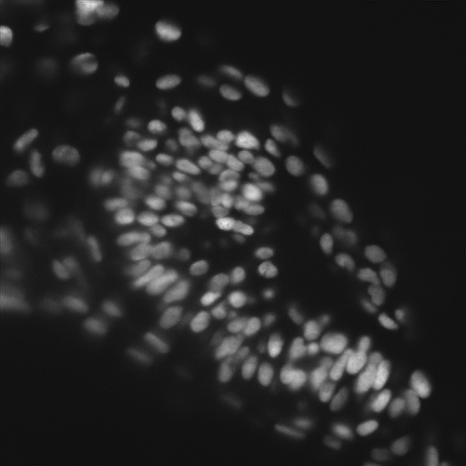
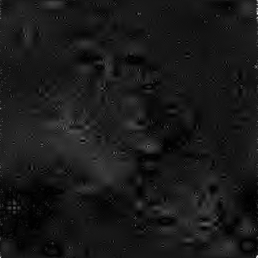
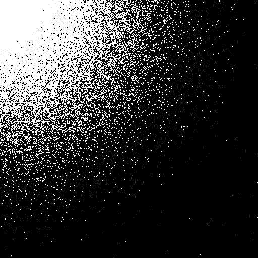
$512\!\times\!512$ 15% $U_{\mathrm{Had}}$$\cdot$$V_{\mathrm{dwt}}^{-1}$ Compressive Imaging, Hadamard Spectroscopy
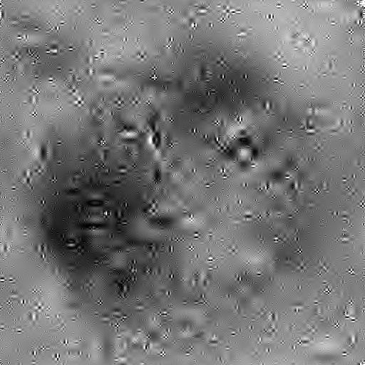
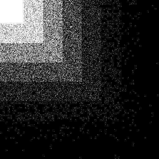
$1024\!\times\!1024$ 20% $U_{\mathrm{dft}}$$\cdot$$V_{\mathrm{dwt}}^{-1}$ Magnetic Resonance Imaging
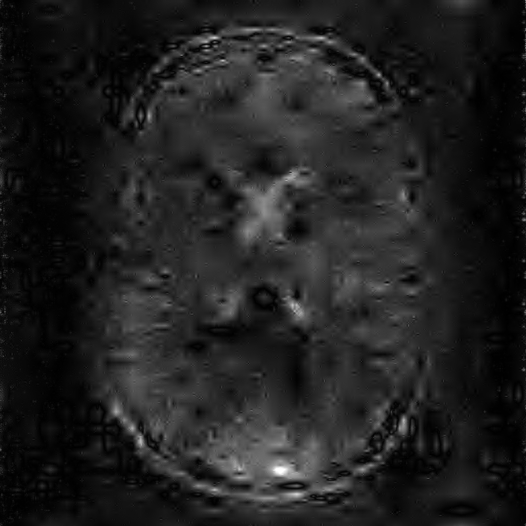
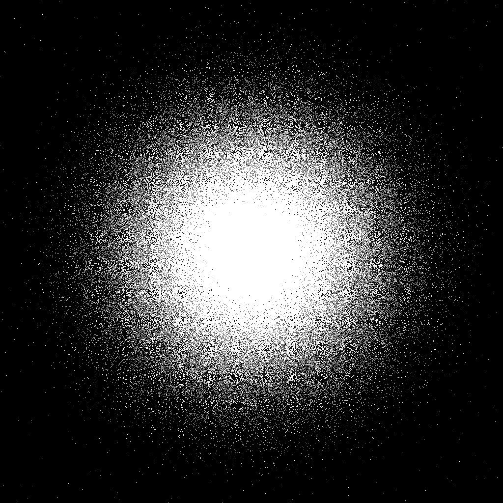
$512\!\times\!512$ 12% $U_{\mathrm{dft}}$$\cdot$$V_{\mathrm{dwt}}^{-1}$ Tomography, Electron Microscopy
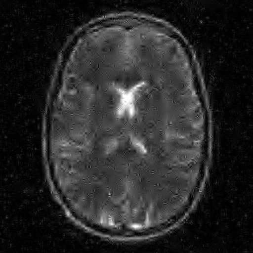
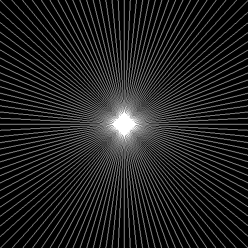
$512\!\times\!512$ 15% $U_{\mathrm{dft}}$$\cdot$$V_{\mathrm{dwt}}^{-1}$ Radio interferometry

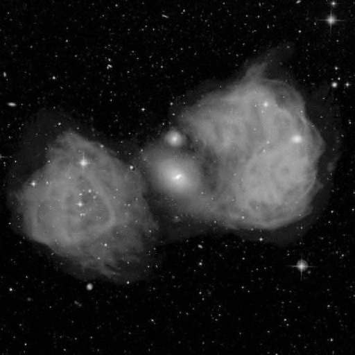
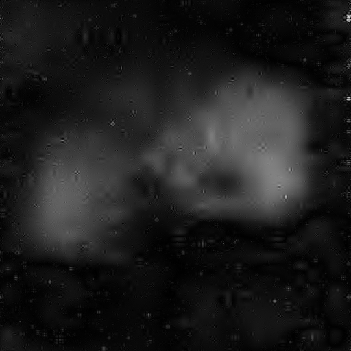
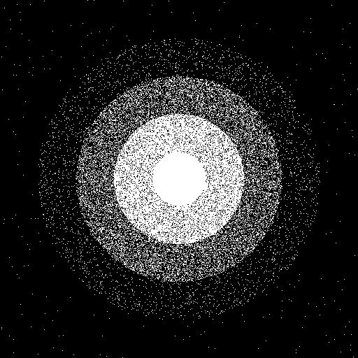
Figure 2: Reconstructions via CS (left column) and the flipped wavelet coefficients (middle column). The right column shows the subsampling map used. The percentage shown is the fraction of Fourier or Hadamard coefficients that were sampled. The reconstruction basis was DB4 for the Fluorescence microscopy example, and DB6 for the rest.

The previous discussion demonstrates that we must dispense with the principles of incoherence and uniform random subsampling in order to develop a new theory of CS. We now claim that sparsity must also be replaced with a more general concept. This may come as a surprise to the reader, since sparsity is a central pillar of not just CS, but much of modern signal processing. However, this can be confirmed by a simple experiment we refer to as the flip test.

Sparsity asserts that an unknown vector $x$ has $s$ important coefficients, where the locations can be arbitrary. CS establishes that all $s$-sparse vectors can be recovered from the same sampling strategy. In particular, the sampling strategy is completely independent of the location of these coefficients. The flip test, described next, allows one to evaluate whether this holds in a given application. Let $x\in\mathbb{C}^{N}$ and $U\in\mathbb{C}^{N\times N}$. Next we take samples according to some appropriate subset $\Omega\subseteq\{1,\ldots,N\}$ with $|\Omega|=m$, and solve:

$$\min_{z\in\mathbb{C}^{N}}\|z\|_{1}\ \mbox{subject to $P_{\Omega}Uz=P_{\Omega}Ux$}.$$ (2.6)

This gives a reconstruction $z=z_{1}$. Now we flip $x$ through the operation $x\mapsto x^{\mathrm{fp}}\in\mathbb{C}^{N},$ $x^{\mathrm{fp}}_{1}=x_{N},$ $x^{\mathrm{fp}}_{2}=x_{N-1},\ldots,x^{\mathrm{fp}}_{N}=x_{1},$ giving a new vector $x^{\mathrm{fp}}$ with reversed entries. We next apply the same CS reconstruction to $x^{\mathrm{fp}}$, using the same matrix $U$ and the same subset $\Omega$. That is we solve

$$\min_{z\in\mathbb{C}^{N}}\|z\|_{1}\ \mbox{subject to $P_{\Omega}Uz=P_{\Omega}Ux^{\mathrm{fp}}$}.$$ (2.7)

Let $z$ be a solution of (2.7). In order to get a reconstruction of the original vector $x$, we perform the flipping operation once more and form the final reconstruction $z_{2}=z^{\mathrm{fp}}$.

Suppose now that $\Omega$ is a good sampling pattern for recovering $x$ using the solution $z_{1}$ of (2.6). If sparsity is the key structure that determines such reconstruction quality, then we expect exactly the same quality in the approximation $z_{2}$ obtained via (2.7), since $x^{\mathrm{fp}}$ is merely a permutation of $x$. To investigate whether or not this is true, we consider several examples arising from the following applications: fluorescence microscopy, compressive imaging, MRI, CT, electron microscopy and radio interferometry. These examples are based on the matrix $U=U_{\mathrm{dft}}V_{\mathrm{dwt}}^{-1}$ or $U=U_{\mathrm{Had}}V_{\mathrm{dwt}}^{-1}$, where $U_{\mathrm{dft}}$ is the discrete Fourier transform, $U_{\mathrm{Had}}$ is a Hadamard matrix and $V_{\mathrm{dwt}}$ is the discrete wavelet transform.

The results of this experiment are shown in Figure 2. As is evident, in all cases the flipped reconstructions $z_{2}$ are substantially worse than their unflipped counterparts $z_{1}$. Hence, we conclude that sparsity alone does not govern the reconstruction quality, and consequently the success in the unflipped case must also be due in part to the structure of the signal. In other words:

The optimal subsampling strategy depends on the signal structure.

Note that the flip test reveals another interesting phenomenon:

There is no Restricted Isometry Property (RIP).

Suppose the matrix $P_{\Omega}U$ satisfied an RIP for realistic parameter values (i.e. problem size $N$, subsampling percentage $m$, and sparsity $s$) found in applications. Then this would imply recovery of all approximately sparse vectors with the same error. This is in direct contradiction with the results of the flip test.

Note that in all the examples in Figure 2, uniform random subsampling would have given nonsensical results, analogously to what was shown in Figure 1.

2.4 Signals and images are asymptotically sparse in -lets

Given that structure is key, we now ask the question: what, if any, structure is characteristic of such applications? Let us consider a wavelet basis $\{\varphi_{n}\}_{n\in\mathbb{N}}$. Recall that associated to such a basis, there is a natural decomposition of $\mathbb{N}$ into finite subsets according to different scales, i.e. $\mathbb{N}=\bigcup_{k\in\mathbb{N}}\{M_{k-1}+1,\ldots,M_{k}\},$ where $0=M_{0}<M_{1}<M_{2}<\ldots$ and $\{M_{k-1}+1,\ldots,M_{k}\}$ is the set of indices corresponding to the $k^{\mathrm{th}}$ scale. Let $x\in l^{2}(\mathbb{N})$ be the coefficients of a function $f$ in this basis. Suppose that $\epsilon\in(0,1]$ is given, and define

$$s_{k}=s_{k}(\epsilon)=\min\Big{\{}K:\Big{\|}\sum_{i=1}^{K}x_{\pi(i)}\varphi_{\pi(i)}\Big{\|}\geq\epsilon\,\Big{\|}\sum_{i=M_{k-1}+1}^{M_{k}}x_{j}\varphi_{j}\Big{\|}\,\Big{\}},$$ (2.8)

where $\pi:\{1,\ldots,M_{k}-M_{k-1}\}\rightarrow\{M_{k-1}+1,\ldots,M_{k}\}$ is a bijection such that $|x_{\pi(i)}|\geq|x_{\pi(i+1)}|$ for $i=1,\ldots,M_{k}-M_{k-1}-1$. In order words, the quantity $s_{k}$ is the effective sparsity of the wavelet coefficients of $f$ at the $k^{\mathrm{th}}$ scale.

Sparsity of $f$ in a wavelet basis means that for a given maximal scale $r\in\mathbb{N}$, the ratio $s/M_{r}\ll 1$, where $M=M_{r}$ and $s=s_{1}+\ldots+s_{r}$ is the total effective sparsity of $f$. The observation that typical images and signals are approximately sparse in wavelet bases is one of the key results in nonlinear approximation [23, 47]. However, such objects exhibit far more than sparsity alone. In fact, the ratios

$$s_{k}/(M_{k}-M_{k-1})\rightarrow 0,$$ (2.9)

rapidly as $k\rightarrow\infty$, for every fixed $\epsilon\in(0,1]$. Thus typical signals and images have a distinct sparsity structure. They are much more sparse at fine scales (large $k$) than at coarse scales (small $k$). This is confirmed in Figure 3. Note that this conclusion does not change if one replaces wavelets by other related approximation systems, such as curvelets [9, 11], contourlets [24, 49] or shearlets [18, 19, 41].

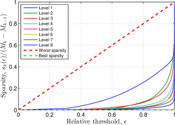
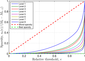
Figure 3: Relative sparsity of the Daubechies-8 wavelet coefficients of two images. Here the levels correspond to wavelet scales and $s_{k}(\epsilon)$ is given by (2.8). Each curve shows the relative sparsity at level $k$ as a function of $\epsilon$. The decreasing nature of the curves for increasing $k$ confirms (2.9).

3 New principles

Having argued for their need, we now introduce the main new concepts of the paper: namely, asymptotic incoherence, asymptotic sparsity and multilevel sampling.

3.1 Asymptotic incoherence

Recall from §2.2 that the case of Fourier sampling with wavelets as the sparsity basis is a standard example of a coherent problem. Similarly, Fourier sampling with Legendre polynomials is also coherent, as is the case of Hadamard sampling with wavelets. In Figure 4 we plot the absolute values of the entries of the matrix $U$ for these three examples. As is evident, whilst $U$ does indeed have large entries in all three case (since it is coherent), these are isolated to a leading submatrix (note that we enumerate over $\mathbb{Z}$ for the Fourier sampling basis and $\mathbb{N}$ for the wavelet/Legendre sparsity bases). As one moves away from this region the values get progressively smaller. That is, the matrix $U$ is incoherent aside from a leading coherent submatrix. This motivates the following definition:

Figure 4: The absolute values of the matrix $U$ in (2.5): (left): DB2 wavelets with Fourier sampling. (middle): Legendre polynomials with Fourier sampling. (right): The absolute values of $U_{\mathrm{Had}}V^{-1}_{\mathrm{dwt}},$ where $U_{\mathrm{Had}}$ is a Hadamard matrix and $V^{-1}_{\mathrm{dwt}}$ is the discrete Haar transform. Light regions correspond to large values and dark regions to small values.

Definition 3.1 (Asymptotic incoherence).

Let be $\{U_{N}\}$ be a sequence of isometries with $U_{N}\in\mathbb{C}^{N}$ or let $U\in\mathcal{B}(l^{2}(\mathbb{N}))$ be an isometry. Then

• $\{U_{N}\}$ is asymptotically incoherent if $\mu(P^{\perp}_{K}U_{N}),\ \mu(U_{N}P^{\perp}_{K})\rightarrow 0,$ when $K\rightarrow\infty,$ with $N/K=c,$ for all $c\geq 1$.

• $U$ is asymptotically incoherent if $\mu(P^{\perp}_{K}U),\ \mu(UP^{\perp}_{K})\rightarrow 0,$ when $K\rightarrow\infty.$

Here $P_{K}$ is the projection onto $\mathrm{span}\{e_{j}:j=1,...,K\}$, where $\{e_{j}\}$ is the canonical basis of either $\mathbb{C}^{N}$ or $l^{2}(\mathbb{N})$, and $P^{\perp}_{K}$ is its orthogonal complement.

In other words, $U$ is asymptotically incoherent if the coherences of the matrices formed by replacing either the first $K$ rows or columns of $U$ are small. As it transpires, the Fourier/wavelets, Fourier/Legendre and Hadamard/wavelets problems are asymptotically incoherent. In particular, $\mu(P^{\perp}_{K}U),\ \mu(UP^{\perp}_{K})=\mathcal{O}\left(K^{-1}\right)$ as $K\rightarrow\infty$ for the former (see §6).

3.2 Multi-level sampling

Asymptotic incoherence suggests a different subsampling strategy should be used instead of uniform random sampling. High coherence in the first few rows of $U$ means that important information about the signal to be recovered may well be contained in its corresponding measurements. Hence to ensure good recovery we should fully sample these rows. Conversely, once outside of this region, when the coherence starts to decrease, we can begin to subsample. Let $N_{1},N,m\in\mathbb{N}$ be given. This now leads us to consider an index set $\Omega$ of the form $\Omega=\Omega_{1}\cup\Omega_{2}$, where $\Omega_{1}=\{1,\ldots,N_{1}\}$, and $\Omega_{2}\subseteq\{N_{1}+1,\ldots,N\}$ is chosen uniformly at random with $|\Omega_{2}|=m$. We refer to this as a two-level sampling scheme. As we shall prove later, the amount of subsampling possible (i.e. the parameter $m$) in the region corresponding to $\Omega_{2}$ will depend solely on the sparsity of the signal and coherence $\mu(P^{\perp}_{N_{1}}U)$.

The two-level scheme represents the simplest type of nonuniform density sampling. There is no reason, however, to restrict our attention to just two levels, full and subsampled. In general, we shall consider multilevel schemes, defined as follows:

Definition 3.2 (Multilevel random sampling).

Let $r\in\mathbb{N}$, $\mathbf{N}=(N_{1},\ldots,N_{r})\in\mathbb{N}^{r}$ with $1\leq N_{1}<\ldots<N_{r}$, $\mathbf{m}=(m_{1},\ldots,m_{r})\in\mathbb{N}^{r}$, with $m_{k}\leq N_{k}-N_{k-1}$, $k=1,\ldots,r$, and suppose that $\Omega_{k}\subseteq\{N_{k-1}+1,\ldots,N_{k}\},\quad|\Omega_{k}|=m_{k},\quad k=1,\ldots,r,$ are chosen uniformly at random, where $N_{0}=0$. We refer to the set $\Omega=\Omega_{\mathbf{N},\mathbf{m}}=\Omega_{1}\cup\ldots\cup\Omega_{r}.$ as an $(\mathbf{N},\mathbf{m})$-multilevel sampling scheme.

Note that the idea of sampling the low-order coefficients of an image differently goes back to the early days of CS. In particular, Donoho considers a two-level approach for recovering wavelet coefficients in his seminal paper [25], based on acquiring the coarse scale coefficients directly. This was later extended by Tsaig & Donoho to so-called ‘multiscale CS’ in [60], where distinct subbands were sensed separately. See also Romberg’s work [54], and as well as Candès & Romberg [13].

We also remark that, although motivated by wavelets, our definition is completely general, as are the theorems we present in §4 and §5. Moreover, and critically, we do not assume separation of the coefficients into distinct levels before sampling (as done above), which is often infeasible in practice (in particular, any application based on Fourier or Hadamard sampling). Note also that in MRI similar sampling strategies to what we introduce here are found in most implementations of CS [45, 46, 51, 52]. Additionally, a so-called “half-half” scheme (an example of a two-level strategy) was used by [57] in application of CS in fluorescence microscopy, albeit without theoretical recovery guarantees.

3.3 Asymptotic sparsity in levels

The flip test, the discussion in §2.4 and Figure 3 suggest that we need a different concept to sparsity. Given the structure of modern function systems such as wavelets and their generalizations, we propose the notion of sparsity in levels:

Definition 3.3 (Sparsity in levels).

Let $x$ be an element of either $\mathbb{C}^{N}$ or $l^{2}(\mathbb{N})$. For $r\in\mathbb{N}$ let $\mathbf{M}=(M_{1},\ldots,M_{r})\in\mathbb{N}^{r}$ with $1\leq M_{1}<\ldots<M_{r}$ and $\mathbf{s}=(s_{1},\ldots,s_{r})\in\mathbb{N}^{r}$, with $s_{k}\leq M_{k}-M_{k-1}$, $k=1,\ldots,r$, where $M_{0}=0$. We say that $x$ is $(\mathbf{s},\mathbf{M})$-sparse if, for each $k=1,\ldots,r$, $\Delta_{k}:=\mathrm{supp}(x)\cap\{M_{k-1}+1,\ldots,M_{k}\},$ satisfies $|\Delta_{k}|\leq s_{k}$. We denote the set of $(\mathbf{s},\mathbf{M})$-sparse vectors by $\Sigma_{\mathbf{s},\mathbf{M}}$.

Definition 3.4 ($(\mathbf{s},\mathbf{M}$)-term approximation).

Let $f=\sum_{j}x_{j}\varphi_{j}$, where $\{\varphi_{j}\}$ is some orthonormal basis of a Hilbert space and $x=(x_{j})$ is an element of either $\mathbb{C}^{N}$ or $l^{2}(\mathbb{N})$. We define the ($\mathbf{s},\mathbf{M}$)-term approximation

$$\sigma_{\mathbf{s},\mathbf{M}}(f)=\min_{\eta\in\Sigma_{\mathbf{s},\mathbf{M}}}\|x-\eta\|_{l^{1}}.$$ (3.1)

Typically, it is the case that $s_{k}/(M_{k}-M_{k-1})\rightarrow 0$ as $k\rightarrow\infty$, in which case we say that $x$ is asymptotically sparse in levels.

4 Main theorems I: the finite-dimensional case

We now present the main theorems in the finite-dimensional setting. In §5 we address the infinite-dimensional case. To avoid pathological examples we will assume throughout that the total sparsity $s=s_{1}+\ldots+s_{r}\geq 3$. This is simply to ensure that $\log(s)\geq 1$, which is convenient in the proofs.

4.1 Two-level sampling schemes

We commence with the case of two-level sampling schemes. Recall that in practice, signals are never exactly sparse (or sparse in levels), and their measurements are always contaminated by noise. Let $f=\sum_{j}x_{j}\varphi_{j}$ be a fixed signal, and write $y=P_{\Omega}\hat{f}+z=P_{\Omega}Ux+z,$ for its noisy measurements, where $z\in\mathrm{ran}(P_{\Omega})$ is a noise vector satisfying $\|z\|\leq\delta$ for some $\delta\geq 0$. If $\delta$ is known, we now consider the following problem:

$$\min_{\eta\in\mathbb{C}^{N}}\|\eta\|_{l^{1}}\ \mbox{subject to $\|P_{\Omega}U\eta-y\|\leq\delta$.}$$ (4.1)

Our aim now is to recover $x$ up to an error proportional to $\delta$ and the best approximation error $\sigma_{\mathbf{s},\mathbf{M}}(f)$.

Before stating our theorem, it is useful to make the following definition. For $K\in\mathbb{N}$, we write $\mu_{K}=\mu(P^{\perp}_{K}U)$. We now have the following:

Theorem 4.1.

Let $U\in\mathbb{C}^{N\times N}$ be an isometry and $x\in\mathbb{C}^{N}$. Suppose that $\Omega=\Omega_{\mathbf{N},\mathbf{m}}$ is a two-level sampling scheme, where $\mathbf{N}=(N_{1},N_{2})$, $N_{2}=N$, and $\mathbf{m}=(N_{1},m_{2})$. Let $(\mathbf{s},\mathbf{M})$, where $\mathbf{M}=(M_{1},M_{2})\in\mathbb{N}^{2}$, $M_{1}<M_{2}$, $M_{2}=N$, and $\mathbf{s}=(M_{1},s_{2})\in\mathbb{N}^{2}$, $s_{2}\leq M_{2}-M_{1}$, be any pair such that the following holds:

1. we have

   $$\|P^{\perp}_{N_{1}}UP_{M_{1}}\|\leq\frac{\gamma}{\sqrt{M_{1}}}$$ (4.2)

   and $\gamma\leq s_{2}\sqrt{\mu_{N_{1}}}$ for some $\gamma\in(0,2/5]$;

2. for $\epsilon\in(0,e^{-1}]$, let

   $$m_{2}\gtrsim(N-N_{1})\cdot\log(\epsilon^{-1})\cdot\mu_{N_{1}}\cdot s_{2}\cdot\log\left(N\right).$$

Suppose that $\xi\in\mathbb{C}^{N}$ is a minimizer of (4.1) with $\delta=\tilde{\delta}\sqrt{K^{-1}}$ and $K=(N_{2}-N_{1})/m_{2}$. Then, with probability exceeding $1-s\epsilon$, we have

$$\|\xi-x\|\leq C\cdot\left(\tilde{\delta}\cdot\left(1+L\cdot\sqrt{s}\right)+\sigma_{\mathbf{s},\mathbf{M}}(f)\right),$$ (4.3)

for some constant $C$, where $\sigma_{\mathbf{s},\mathbf{M}}(f)$ is as in (3.1), $L=1+\frac{\sqrt{\log_{2}\left(6\epsilon^{-1}\right)}}{\log_{2}(4KM\sqrt{s})}$. If $m_{2}=N-N_{1}$ then this holds with probability $1$.

To interpret Theorem 4.1, and in particular, show how it overcomes the coherence barrier, we note the following:

1. The condition $\|P_{N_{1}}^{\perp}UP_{M_{1}}\|\leq\frac{2}{5\sqrt{M_{1}}}$ (which is always satisfied for some $N_{1}$) implies that fully sampling the first $N_{1}$ measurements allows one to recover the first $M_{1}$ coefficients of $f$.

2. To recover the remaining $s_{2}$ coefficients we require, up to log factors, an additional $m_{2}\gtrsim(N-N_{1})\cdot\mu_{N_{1}}\cdot s_{2},$ measurements, taken randomly from the range $M_{1}+1,\ldots,M_{2}$. In particular, if $N_{1}$ is a fixed fraction of $N$, and if $\mu_{N_{1}}=\mathcal{O}\left(N^{-1}_{1}\right)$, such as for wavelets with Fourier measurements (Theorem 6.1), then one requires only $m_{2}\gtrsim s_{2}$ additional measurements to recover the sparse part of the signal.

Thus, in the case where $x$ is asymptotically sparse, we require a fixed number $N_{1}$ measurements to recover the nonsparse part of $x$, and then a number $m_{2}$ depending on $s_{2}$ and the asymptotic coherence $\mu_{N_{1}}$ to recover the sparse part.

• It is not necessary to know the sparsity structure, i.e. the values $\mathbf{s}$ and $\mathbf{M}$, of the signal $f$ in order to implement the two-level sampling technique (the same also applies to the multilevel technique discussed in the next section). Given a two-level scheme $\Omega=\Omega_{\mathbf{N},\mathbf{m}}$, Theorem 4.1 demonstrates that $f$ will be recovered exactly up to an error on the order of $\sigma_{\mathbf{s},\mathbf{M}}(f)$, where $\mathbf{s}$ and $\mathbf{M}$ are determined implicitly by $\mathbf{N}$, $\mathbf{m}$ and the conditions (i) and (ii) of the theorem. Of course, some a priori knowledge of $\mathbf{s}$ and $\mathbf{M}$ will greatly assist in selecting the parameters $\mathbf{N}$ and $\mathbf{m}$ so as to get the best recovery results. However, this is not strictly necessary for implementation.

4.2 Multilevel sampling schemes

We now consider the case of multilevel sampling schemes. Before presenting this case, we need several definitions. The first is key concept in this paper: namely, the local coherence.

Definition 4.2 (Local coherence).

Let $U$ be an isometry of either $\mathbb{C}^{N}$ or $l^{2}(\mathbb{N})$. If $\mathbf{N}=(N_{1},\ldots,N_{r})\in\mathbb{N}^{r}$ and $\mathbf{M}=(M_{1},\ldots,M_{r})\in\mathbb{N}^{r}$ with $1\leq N_{1}<\ldots N_{r}$ and $1\leq M_{1}<\ldots<M_{r}$ the $(k,l)^{\mathrm{th}}$ local coherence of $U$ with respect to $\mathbf{N}$ and $\mathbf{M}$ is given by

$$\mu_{\mathbf{N},\mathbf{M}}(k,l) =\sqrt{\mu(P^{N_{k-1}}_{N_{k}}UP^{M_{l-1}}_{M_{l}})\cdot\mu(P^{N_{k-1}}_{N_{k}}U)},\quad k,l=1,\ldots,r,$$

where $N_{0}=M_{0}=0$ and $P^{a}_{b}$ denotes the projection matrix corresponding to indices $\{a+1,\ldots,b\}$. In the case where $U\in\mathcal{B}(l^{2}(\mathbb{N}))$ (i.e. $U$ belongs to the space of bounded operators on $l^{2}(\mathbb{N})$), we also define

$$\mu_{\mathbf{N},\mathbf{M}}(k,\infty) =\sqrt{\mu(P^{N_{k-1}}_{N_{k}}UP_{M_{r-1}}^{\perp})\cdot\mu(P^{N_{k-1}}_{N_{k}}U)},\quad k=1,\ldots,r.$$

Besides the local sparsities $s_{k}$, we shall also require the notion of a relative sparsity:

Definition 4.3 (Relative sparsity).

Let $U$ be an isometry of either $\mathbb{C}^{N}$ or $l^{2}(\mathbb{N})$. For $\mathbf{N}=(N_{1},\ldots,N_{r})\in\mathbb{N}^{r}$, $\mathbf{M}=(M_{1},\ldots,M_{r})\in\mathbb{N}^{r}$ with $1\leq N_{1}<\ldots<N_{r}$ and $1\leq M_{1}<\ldots<M_{r}$, $\mathbf{s}=(s_{1},\ldots,s_{r})\in\mathbb{N}^{r}$ and $1\leq k\leq r$, the $k^{\mathrm{th}}$ relative sparsity is given by $S_{k}=S_{k}(\mathbf{N},\mathbf{M},\mathbf{s})=\max_{\eta\in\Theta}\|P_{N_{k}}^{N_{k-1}}U\eta\|^{2},$ where $N_{0}=M_{0}=0$ and $\Theta$ is the set

$$\Theta=\{\eta:\|\eta\|_{l^{\infty}}\leq 1,|\mathrm{supp}(P_{M_{l}}^{M_{l-1}}\eta)|=s_{l},\,l=1,\ldots,r\}.$$

We can now present our main theorem:

Theorem 4.4.

Let $U\in\mathbb{C}^{N\times N}$ be an isometry and $x\in\mathbb{C}^{N}$. Suppose that $\Omega=\Omega_{\mathbf{N},\mathbf{m}}$ is a multilevel sampling scheme, where $\mathbf{N}=(N_{1},\ldots,N_{r})\in\mathbb{N}^{r}$, $N_{r}=N$, and $\mathbf{m}=(m_{1},\ldots,m_{r})\in\mathbb{N}^{r}$. Let $(\mathbf{s},\mathbf{M})$, where $\mathbf{M}=(M_{1},\ldots,M_{r})\in\mathbb{N}^{r}$, $M_{r}=N$, and $\mathbf{s}=(s_{1},\ldots,s_{r})\in\mathbb{N}^{r}$, be any pair such that the following holds: for $\epsilon\in(0,e^{-1}]$ and $1\leq k\leq r$,

$$1\gtrsim\frac{N_{k}-N_{k-1}}{m_{k}}\cdot\log(\epsilon^{-1})\cdot\left(\sum_{l=1}^{r}\mu_{\mathbf{N},\mathbf{M}}(k,l)\cdot s_{l}\right)\cdot\log\left(N\right),$$ (4.4)

where $m_{k}\gtrsim\hat{m}_{k}\cdot\log(\epsilon^{-1})\cdot\log\left(N\right),$ and $\hat{m}_{k}$ is such that

$$1\gtrsim\sum_{k=1}^{r}\left(\frac{N_{k}-N_{k-1}}{\hat{m}_{k}}-1\right)\cdot\mu_{\mathbf{N},\mathbf{M}}(k,l)\cdot\tilde{s}_{k},$$ (4.5)

for all $l=1,\ldots,r$ and all $\tilde{s}_{1},\ldots,\tilde{s}_{r}\in(0,\infty)$ satisfying

$$\tilde{s}_{1}+\ldots+\tilde{s}_{r}\leq s_{1}+\ldots+s_{r},\qquad\tilde{s}_{k}\leq S_{k}(\mathbf{N},\mathbf{M},\mathbf{s}).$$

Suppose that $\xi\in\mathbb{C}^{N}$ is a minimizer of (4.1) with $\delta=\tilde{\delta}\sqrt{K^{-1}}$ and $K=\max_{1\leq k\leq r}\{(N_{k}-N_{k-1})/m_{k}\}$. Then, with probability exceeding $1-s\epsilon$, where $s=s_{1}+\ldots+s_{r}$, we have that

$$\|\xi-x\|\leq C\cdot\left(\tilde{\delta}\cdot\left(1+L\cdot\sqrt{s}\right)+\sigma_{\mathbf{s},\mathbf{M}}(f)\right),$$

for some constant $C$, where $\sigma_{\mathbf{s},\mathbf{M}}(f)$ is as in (3.1), $L=1+\frac{\sqrt{\log_{2}\left(6\epsilon^{-1}\right)}}{\log_{2}(4KM\sqrt{s})}$. If $m_{k}=N_{k}-N_{k-1}$, $1\leq k\leq r$, then this holds with probability $1$.

The key component of this theorem is the bounds (4.4) and (4.5). Whereas the standard CS estimate (2.2) relates the total number of samples $m$ to the global coherence and the global sparsity, these bounds now relate the local sampling $m_{k}$ to the local coherences $\mu_{\mathbf{N},\mathbf{M}}(k,l)$ and local and relative sparsities $s_{k}$ and $S_{k}$. In particular, by relating these local quantities this theorem conforms with the conclusions of the flip test in §2.3: namely, that the optimal sampling strategy must depend on the signal structure. This is exactly what is described in (4.4) and (4.5).

On the face of it, the bounds (4.4) and (4.5) may appear somewhat complicated, not least because they involve the relative sparsities $S_{k}$. As we next show, however, they are indeed sharp in the sense that they reduce to the correct information-theoretic limits in several important cases. Furthermore, in the important case of wavelet sparsity with Fourier sampling, they can be used to provide near-optimal recovery guarantees. We discuss this in §6. Note, however, that to do this it is first necessary to generalize Theorem 4.4 to the infinite-dimensional setting, which we do in §5.

4.2.1 Sharpness of the estimates – the block-diagonal case

Suppose that $\Omega=\Omega_{\mathbf{N},\mathbf{m}}$ is a multilevel sampling scheme, where $\mathbf{N}=(N_{1},\ldots,N_{r})\in\mathbb{N}^{r}$ and $\mathbf{m}=(m_{1},\ldots,m_{r})\in\mathbb{N}^{r}$. Let $(\mathbf{s},\mathbf{M})$, where $\mathbf{M}=(M_{1},\ldots,M_{r})\in\mathbb{N}^{r}$, and suppose for simplicity that $\mathbf{M}=\mathbf{N}$. Consider the block-diagonal matrix

$$A=A_{1}\oplus\ldots\oplus A_{r}\in\mathbb{C}^{N\times N},\quad A_{k}\in\mathbb{C}^{(N_{k}-N_{k-1})\times(N_{k}-N_{k-1})},\quad A_{k}^{*}A_{k}=I,$$

where $N_{0}=0$. Note that in this setting we have $S_{k}=s_{k},$ $\mu_{\mathbf{N},\mathbf{M}}(k,l)=0,$ $k\neq l.$ Also, since $\mu(\mathbf{N},\mathbf{M})(k,k)=\mu(A_{k})$, equations (4.4) and (4.5) reduce to

$$1\gtrsim\frac{N_{k}-N_{k-1}}{m_{k}}\cdot\log(\epsilon^{-1})\cdot\mu(A_{k})\cdot s_{k}\cdot\log(N),\quad 1\gtrsim\left(\frac{N_{k}-N_{k-1}}{\hat{m}_{k}}-1\right)\cdot\mu(A_{k})\cdot s_{k}.$$

In particular, it suffices to take

$$m_{k}\gtrsim(N_{k}-N_{k-1})\cdot\log(\epsilon^{-1})\cdot\mu(A_{k})\cdot s_{k}\cdot\log(N),\quad 1\leq k\leq r.$$ (4.6)

This is exactly as one expects: the number of measurements in the $k^{\mathrm{th}}$ level depends on the size of the level multiplied by the local coherence and the sparsity in that level. Note that this result recovers the standard one-level results in finite dimensions [1, 12] up to a slight deterioration in the probability bound to $1-s\epsilon$. Specifically, the usual bound would be $1-\epsilon$. The question as to whether or not this $s$ can be removed in the multilevel setting is open, although such a result would be more of a cosmetic improvement.

4.2.2 Sharpness of the estimates – the non-block diagonal case

The previous argument demonstrated that Theorem 4.4 is sharp, up to the probability term, in the sense that it reduces to the usual estimate (4.6) for block-diagonal matrices, i.e. $S_{k}=s_{k}$. This is not true in the general setting. Clearly, $S_{k}\leq s=s_{1}+\ldots+s_{r}.$ However in general there is usually interference between different sparsity levels, which means that $S_{k}$ need not have anything to do with $s_{k}$, or can indeed be proportional to the total sparsity $s$. This may seem an undesirable aspect of the theorems, since $S_{k}$ may be significantly larger than $s_{k}$, and thus the estimate on the number of measurements $m_{k}$ required in the $k^{\mathrm{th}}$ level may also be much larger than the corresponding sparsity $s_{k}$. Could it therefore be that the $S_{k}$s are an unfortunate artefact of the proof? As we now show by example, this is not the case.

Let $N=rn$ for some $n\in\mathbb{N}$ and $\mathbf{N}=\mathbf{M}=(n,2n,\ldots,rn)$. Let $W\in\mathbb{C}^{n\times n}$ and $V\in\mathbb{C}^{r\times r}$ be isometries and consider the matrix

$$A=V\otimes W,$$

where $\otimes$ is the usual Kronecker product. Note that $A\in\mathbb{C}^{N\times N}$ is also an isometry. Now suppose that $x=(x_{1},\ldots,x_{r})\in\mathbb{C}^{N}$ is an $(\mathbf{s},\mathbf{M})$-sparse vector, where each $x_{k}\in\mathbb{C}^{n}$ is $s_{k}$-sparse. Then $Ax=y,\quad y=(y_{1},\ldots,y_{r}),\ y_{k}=Wz_{k},\ z_{k}=\sum^{r}_{l=1}v_{kl}x_{l}.$ Hence the problem of recovering $x$ from measurements $y$ with an $(\mathbf{N},\mathbf{m})$-multilevel strategy decouples into $r$ problems of recovering the vector $z_{k}$ from the measurements $y_{k}=Wz_{k}$, $k=1,\ldots,r$. Let $\hat{s}_{k}$ denote the sparsity of $z_{k}$. Since the coherence provides an information-theoretic limit [12], one requires at least

$$m_{k}\gtrsim n\cdot\mu(W)\cdot\hat{s}_{k}\cdot\log(n),\quad 1\leq k\leq r.$$ (4.7)

measurements at level $k$ in order to recover each $z_{k}$, and therefore recover $x$, regardless of the reconstruction method used. We now consider two examples of this setup:

• Let $\pi:\{1,\ldots,r\}\rightarrow\{1,\ldots,r\}$ be a permutation and let $V$ be the matrix with entries $v_{kl}=\delta_{l,\pi(k)}$. Since $z_{k}=x_{\pi(k)}$ in this case, the lower bound (4.7) reads

  $$m_{k}\gtrsim n\cdot\mu(W)\cdot s_{\pi(k)}\cdot\log(n),\quad 1\leq k\leq r.$$ (4.8)

  Now consider Theorem 4.4 for this matrix. First, we note that $S_{k}=s_{\pi(k)}$. In particular, $S_{k}$ is completely unrelated to $s_{k}$. Substituting this into Theorem 4.4 and noting that $\mu_{\mathbf{N},\mathbf{M}}(k,l)=\mu(W)\delta_{l,\pi(k)}$ in this case, we arrive at the condition $m_{k}\gtrsim n\cdot\mu(W)\cdot s_{\pi(k)}\cdot\left(\log(\epsilon^{-1})+1\right)\cdot\log(nr),$ which is equivalent to (4.8) provided $r\lesssim n$.

• Now suppose that $V$ is the $r\times r$ DFT matrix. Suppose also that $s\leq n/r$ and that the $x_{k}$’s have disjoint support sets, i.e. $\mathrm{supp}(x_{k})\cap\mathrm{supp}(x_{l})=\emptyset$, $k\neq l$. Then by construction, each $z_{k}$ is $s$-sparse, and therefore the lower bound (4.7) reads $m_{k}\gtrsim n\cdot\mu(W)\cdot s\cdot\log n,$ for $1\leq k\leq r.$ After a short argument, one finds that $s/r\leq S_{k}\leq s$ in this case. Hence, $S_{k}$ is typically much larger than $s_{k}$. Moreover, after noting that $\mu_{\mathbf{N},\mathbf{M}}(k,l)=\frac{1}{r}\mu(W)$, we find that Theorem 4.4 gives the condition $m_{k}\gtrsim n\cdot\mu(W)\cdot s\cdot\left(\log(\epsilon^{-1})+1\right)\cdot\log(nr).$ Thus, Theorem 4.4 obtains the lower bound in this case as well.

4.2.3 Sparsity leads to pessimistic reconstruction guarantees

The flip test demonstrates that any sparsity-based theory of CS cannot describe the quality of the reconstructions seen in practice. To conclude this section, we now use the block-diagonal case to further emphasize the need for theorems that go beyond sparsity, such as Theorems 4.1 and 4.4. To see this, consider the block-diagonal matrix

$$U=U_{1}\oplus\ldots\oplus U_{r},\qquad U_{k}\in\mathbb{C}^{(N_{k}-N_{k-1})\times(N_{k}-N_{k-1})},$$

where each $U_{k}$ is perfectly incoherent, i.e. $\mu(U_{k})=(N_{k}-N_{k-1})^{-1}$, and suppose we take $m_{k}$ measurements within each block $U_{k}$. Let $x\in\mathbb{C}^{N}$ be the signal we wish to recover, where $N=N_{r}$. The question is, how many samples $m=m_{1}+\ldots+m_{r}$ do we require?

Suppose we assume that $x$ is $s$-sparse, where $s\leq\min_{k=1,\ldots,r}\{N_{k}-N_{k-1}\}$. Given no further information about the sparsity structure, it is necessary to take $m_{k}\gtrsim s\log(N)$ measurements in each block, giving $m\gtrsim rs\log(N)$ in total. However, suppose now that $x$ is known to be $s_{k}$-sparse within each level, i.e. $|\mathrm{supp}(x)\cap\{N_{k-1}+1,\ldots,N_{k}\}|=s_{k}.$ Then we now require only $m_{k}\gtrsim s_{k}\log(N)$, and therefore $m\gtrsim s\log(N)$ total measurements. Thus, structured sparsity leads to a significant saving by a factor of $r$ in the total number of measurements required.

Although this may appear insignificant on the face of it, this factor represents a substantial saving in practice. Given that a $512\times 512$ image corresponds to $r=9$ wavelet scales, any sparsity-based theorem will lead to a nine-fold overestimate in the number of measurements required. Since $m\approx 5-10\%$ are typically necessary in applications (see, for example, Figure 2), such an overestimate, i.e. $m\approx 45-90\%$, is therefore of little or no practical use. Although this argument is based on a simplified model, the block-diagonal structure described above is a good approximation to the Fourier/wavelets recovery problem, which we discuss in detail in §6.

5 Main theorems II: the infinite-dimensional case

Finite-dimensional CS is suitable in many cases. However, there are some important problems where it can lead to significant problems, since the underlying problem is continuous/analog. Discretization of the problem in order to produce a finite-dimensional, vector-space model can lead to substantial errors [1, 7, 16, 56], due to the phenomenon of model mismatch.

To address this issue, a theory of infinite-dimensional CS was introduced by Adcock & Hansen in [1], based on a new approach to classical sampling known as generalized sampling [2, 3, 4, 5, 6, 38]. We describe this theory next. Note that this infinite-dimensional CS model has also been advocated for and implemented in MRI by Guerquin–Kern, Häberlin, Pruessmann & Unser [33]. Note also that sampling theories such as generalized sampling and finite rate of innovation [61] are infinite-dimensional, and hence it is most natural that CS has an infinite-dimensional theory as well.

5.1 Infinite-dimensional CS

Suppose that $\mathcal{H}$ is a separable Hilbert space over $\mathbb{C}$, and let $\{\psi_{j}\}_{j\in\mathbb{N}}$ be an orthonormal basis on $\mathcal{H}$ (the sampling basis). Let $\{\varphi_{j}\}_{j\in\mathbb{N}}$ be an orthonormal system in $\mathcal{H}$ (the sparsity system), and suppose that

$$U=(u_{ij})_{i,j\in\mathbb{N}},\qquad u_{ij}=\langle\varphi_{j},\psi_{i}\rangle,$$ (5.1)

is an infinite matrix. We may consider $U$ as an element of $\mathcal{B}(l^{2}(\mathbb{N}))$; the space of bounded operators on $l^{2}(\mathbb{N})$. As in the finite-dimensional case, $U$ is an isometry, and we may define its coherence $\mu(U)\in(0,1]$ analogously to (2.1). We want to recover $f=\sum_{j\in\mathbb{N}}x_{j}\varphi_{j}\in\mathcal{H}$ from a small number of the measurements $\hat{f}=\{\hat{f}_{j}\}_{j\in\mathbb{N}},$ where $\hat{f}_{j}=\langle f,\psi_{j}\rangle$. To do this, we introduce a second parameter $N\in\mathbb{N}$, and let $\Omega$ be a randomly-chosen subset of indices $1,\ldots,N$ of size $m$. Unlike in finite dimensions, we now consider two cases. Suppose first that $P^{\perp}_{M}x=0$, i.e. $x$ has no tail. Then we solve

$$\inf_{\eta\in l^{1}(\mathbb{N})}\|\eta\|_{l^{1}}\ \mbox{subject to $\|P_{\Omega}UP_{M}\eta-y\|\leq\delta$},$$ (5.2)

where $y=P_{\Omega}\hat{f}+z$ and $z\in\mathrm{ran}(P_{\Omega})$ is a noise vector satisfying $\|z\|\leq\delta$, and $P_{\Omega}$ is the projection operator corresponding to the index set $\Omega$. In [1] it was proved that any solution to (5.2) recovers $f$ exactly up to an error determined by $\sigma_{s,M}(f)$, provided $N$ and $m$ satisfy the so-called weak balancing property with respect to $M$ and $s$ (see Definition 5.1, as well as Remark 5.2 for a discussion), and provided

$$m\gtrsim\mu(U)\cdot N\cdot s\cdot\left(1+\log(\epsilon^{-1})\right)\cdot\log\left(m^{-1}MN\sqrt{s}\right).$$ (5.3)

As in the finite-dimensional case, which turns out to be a corollary of this result, we find that $m$ is on the order of the sparsity $s$ whenever $\mu(U)$ is sufficiently small.

In practice, the condition $P^{\perp}_{M}x=0$ is unrealistic. In the more general case, $P^{\perp}_{M}x\neq 0$, we solve the following problem:

$$\inf_{\eta\in l^{1}(\mathbb{N})}\|\eta\|_{l^{1}}\ \mbox{subject to $\|P_{\Omega}U\eta-y\|\leq\delta$}.$$ (5.4)

In [1] it was shown that any solution of (5.4) recovers $f$ exactly up to an error determined by $\sigma_{s,M}(f)$, provided $N$ and $m$ satisfy the so-called strong balancing property with respect to $M$ and $s$ (see Definition 5.1), and provided a bound similar to (5.3) holds, where the $M$ is replaced by a slightly larger constant (we give the details in the next section in the more general setting of multilevel sampling). Note that (5.4) cannot be solved numerically, since it is infinite-dimensional. Therefore in practice we replace (5.4) by

$$\inf_{\eta\in l^{1}(\mathbb{N})}\|\eta\|_{l^{1}}\ \mbox{subject to $\|P_{\Omega}UP_{R}\eta-y\|\leq\delta$},$$ (5.5)

where $R$ is taken sufficiently large. See [1] for more information.

5.2 Main theorems

We first require the definition of the so-called balancing property [1]:

Definition 5.1 (Balancing property).

Let $U\in\mathcal{B}(l^{2}(\mathbb{N}))$ be an isometry. Then $N\in\mathbb{N}$ and $K\geq 1$ satisfy the weak balancing property with respect to $U,$ $M\in\mathbb{N}$ and $s\in\mathbb{N}$ if

$$\begin{split}\|P_{M}U^{*}P_{N}UP_{M}-P_{M}\|_{l^{\infty}\rightarrow l^{\infty}}\leq\frac{1}{8}\left(\log_{2}^{1/2}\left(4\sqrt{s}KM\right)\right)^{-1},\end{split}$$ (5.6)

where ${\left\|\cdot\right\|}_{l^{\infty}\rightarrow l^{\infty}}$ is the norm on $\mathcal{B}(l^{\infty}(\mathbb{N}))$. We say that $N$ and $K$ satisfy the strong balancing property with respect to $U,$ $M$ and $s$ if (5.6) holds, as well as

$$\begin{split}\|P_{M}^{\perp}U^{*}P_{N}UP_{M}\|_{l^{\infty}\rightarrow l^{\infty}}\leq\frac{1}{8}.\end{split}$$ (5.7)

As in the previous section, we commence with the two-level case. Furthermore, to illustrate the differences between the weak/strong balancing property, we first consider the setting of (5.2):

Theorem 5.2.

Let $U\in\mathcal{B}(l^{2}(\mathbb{N}))$ be an isometry and $x\in l^{1}(\mathbb{N})$. Suppose that $\Omega=\Omega_{\mathbf{N},\mathbf{m}}$ is a two-level sampling scheme, where $\mathbf{N}=(N_{1},N_{2})$ and $\mathbf{m}=(N_{1},m_{2})$. Let $(\mathbf{s},\mathbf{M})$, where $\mathbf{M}=(M_{1},M_{2})\in\mathbb{N}^{2}$, $M_{1}<M_{2}$, and $\mathbf{s}=(M_{1},s_{2})\in\mathbb{N}^{2}$, be any pair such that the following holds:

1. we have $\|P^{\perp}_{N_{1}}UP_{M_{1}}\|\leq\frac{\gamma}{\sqrt{M_{1}}}$ and $\gamma\leq s_{2}\sqrt{\mu_{N_{1}}}$ for some $\gamma\in(0,2/5]$;

2. the parameters $N=N_{2},K=(N_{2}-N_{1})/m_{2}$ satisfy the weak balancing property with respect to $U$, $M:=M_{2}$ and $s:=M_{1}+s_{2}$;

3. for $\epsilon\in(0,e^{-1}]$, let

   $$m_{2}\gtrsim(N-N_{1})\cdot\log(\epsilon^{-1})\cdot\mu_{N_{1}}\cdot s_{2}\cdot\log\left(KM\sqrt{s}\right).$$

Suppose that $P^{\perp}_{M_{2}}x=0$ and let $\xi\in l^{1}(\mathbb{N})$ be a minimizer of (5.2) with $\delta=\tilde{\delta}\sqrt{K^{-1}}$. Then, with probability exceeding $1-s\epsilon$, we have

$$\|\xi-x\|\leq C\cdot\left(\tilde{\delta}\cdot\left(1+L\cdot\sqrt{s}\right)+\sigma_{\mathbf{s},\mathbf{M}}(f)\right),$$ (5.8)

for some constant $C$, where $\sigma_{\mathbf{s},\mathbf{M}}(f)$ is as in (3.1), and $L=1+\frac{\sqrt{\log_{2}\left(6\epsilon^{-1}\right)}}{\log_{2}(4KM\sqrt{s})}$. If $m_{2}=N-N_{1}$ then this holds with probability $1$.

We next state a result for multilevel sampling in the more general setting of (5.4). For this, we require the following notation: $\tilde{M}=\min\{i\in\mathbb{N}:\max_{k\geq i}\|P_{N}Ue_{k}\|\leq 1/(32K\sqrt{s})\},$ where $N$, $s$ and $K$ are as defined below.

Theorem 5.3.

Let $U\in\mathcal{B}(l^{2}(\mathbb{N}))$ be an isometry and $x\in l^{1}(\mathbb{N})$. Suppose that $\Omega=\Omega_{\mathbf{N},\mathbf{m}}$ is a multilevel sampling scheme, where $\mathbf{N}=(N_{1},\ldots,N_{r})\in\mathbb{N}^{r}$ and $\mathbf{m}=(m_{1},\ldots,m_{r})\in\mathbb{N}^{r}$. Let $(\mathbf{s},\mathbf{M})$, where $\mathbf{M}=(M_{1},\ldots,M_{r})\in\mathbb{N}^{r}$, $M_{1}<\ldots<M_{r}$, and $\mathbf{s}=(s_{1},\ldots,s_{r})\in\mathbb{N}^{r}$, be any pair such that the following holds:

1. the parameters $N=N_{r},K=\max_{k=1,\ldots,r}\left\{\frac{N_{k}-N_{k-1}}{m_{k}}\right\},$ satisfy the strong balancing property with respect to $U$, $M:=M_{r}$ and $s:=s_{1}+\ldots+s_{r}$;

2. for $\epsilon\in(0,e^{-1}]$ and $1\leq k\leq r$,

   $$1\gtrsim\frac{N_{k}-N_{k-1}}{m_{k}}\cdot\log(\epsilon^{-1})\cdot\left(\sum_{l=1}^{r}\mu_{\mathbf{N},\mathbf{M}}(k,l)\cdot s_{l}\right)\cdot\log\left(K\tilde{M}\sqrt{s}\right),$$

   (with $\mu_{\mathbf{N},\mathbf{M}}(k,r)$ replaced by $\mu_{\mathbf{N},\mathbf{M}}(k,\infty)$) and $m_{k}\gtrsim\hat{m}_{k}\cdot\log(\epsilon^{-1})\cdot\log\left(K\tilde{M}\sqrt{s}\right),$ where $\hat{m}_{k}$ satisfies (4.5).

Suppose that $\xi\in l^{1}(\mathbb{N})$ is a minimizer of (5.4) with $\delta=\tilde{\delta}\sqrt{K^{-1}}$. Then, with probability exceeding $1-s\epsilon$,

$$\|\xi-x\|\leq C\cdot\left(\tilde{\delta}\cdot\left(1+L\cdot\sqrt{s}\right)+\sigma_{\mathbf{s},\mathbf{M}}(f)\right),$$

for some constant $C$, where $\sigma_{\mathbf{s},\mathbf{M}}(f)$ is as in (3.1), and $L=C\cdot\left(1+\frac{\sqrt{\log_{2}\left(6\epsilon^{-1}\right)}}{\log_{2}(4KM\sqrt{s})}\right).$ If $m_{k}=N_{k}-N_{k-1}$ for $1\leq k\leq r$ then this holds with probability $1$.

This theorem removes the condition in Theorem 5.2 that $x$ has zero tail. Note that the price to pay is the $\tilde{M}$ in the logarithmic term rather than $M$ ($\tilde{M}\geq M$ because of the balancing property). Observe that $\tilde{M}$ is finite, and in the case of Fourier sampling with wavelets, we have that $\tilde{M}=\mathcal{O}\left(KN\right)$ (see §6). Note that Theorem 5.2 has a strong form analogous to Theorem 5.3 which removes the tail condition. The only difference is the requirement of the strong, as opposed to the weak, balancing property, and the replacement of $M$ by $\tilde{M}$ in the log factor. Similarly, Theorem 5.3 has a weak form involving a tail condition. For succinctness we do not state these.

• The balancing property is the main difference between the finite- and infinite-dimensional theorems. Its role is to ensure that the truncated matrix $P_{N}UP_{M}$ is close to an isometry. In reconstruction problems, the presence of an isometry ensures stability in the mapping between measurements and coefficients [2], which explains the need for a such a property in our theorems. As explained in [1], without the balancing property the lack of stability in this mapping leads to numerically useless reconstructions. Note that the balancing property is usually not satisfied for $N=M$. In general, one requires $N>M$ for the balancing property to hold. However, there is always a finite $N$ for which it is satisfied, since the infinite matrix $U$ is an isometry. For details we refer to [1]. We will provide specific estimates in §6 for the required magnitude of $N$ in the case of Fourier sampling with wavelet sparsity.

5.3 The need for infinite-dimensional CS

As mentioned, infinite-dimensional CS is necessary to avoid the artefacts that are introduced when one applies finite-dimensional CS techniques to analog problems. To illustrate this, we consider the problem of recovering a smooth phantom, i.e. a $C^{\infty}$ bivariate function, from its Fourier data. Note that this arises in both electron microscopy and spectroscopy. The test function is $f(x,y)=\cos^{2}(17\pi x/2)\cos^{2}(17\pi y/2)\exp(-x-y)$. In Figure 5, we compare finite-dimensional CS, based on solving (4.1) with $U=U_{\mathrm{dft}}V^{-1}_{\mathrm{dwt}}$ (discrete Fourier and wavelet transform respectively) with infinite-dimensional CS, which solves (5.5) with the Fourier basis $\{\psi_{j}\}_{j\in\mathbb{N}}$ and boundary wavelet basis $\{\varphi_{j}\}_{j\in\mathbb{N}}$. The improvement one gets is due to that fact that that the error in infinite-dimensional case is dominated by the wavelet approximation error, whereas in the finite-dimensional case (due mismatch between the continuous Fourier samples and the discrete Fourier transform) the error is dominated by the Fourier approximation error. As is well known [47], wavelet approximation is superior to Fourier approximation and depends on the number of vanishing moments of the wavelet used (DB4 in this case).

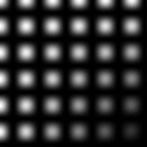
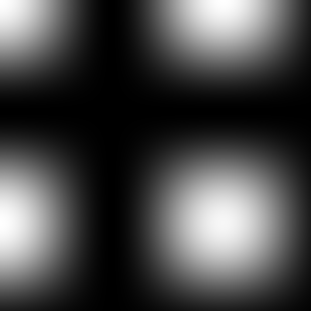
Original	Original (zoomed)	Infinite-dim. CS (zoomed)	Finite-dim. CS (zoomed)
		Err 0.6%	Err 12.7%

Figure 5: Subsampling 6.15%. Both reconstructions are based on identical sampling information.

6 Recovery of wavelet coefficients from Fourier samples

As noted, Fourier sampling with wavelet sparsity is a important reconstruction problem in CS, with numerous applications ranging from medical imaging to seismology and interferometry. Here we consider the Fourier sampling basis $\{\psi_{j}\}_{j\in\mathbb{N}}$ and wavelet reconstruction basis $\{\varphi_{j}\}_{j\in\mathbb{N}}$ (see §7.4.1 for a formal definition) with the infinite matrix $U$ as in (5.1). The incoherence properties can be described as follows.

Theorem 6.1.

Let $U\in\mathcal{B}(l^{2}(\mathbb{N}))$ be the matrix from (7.107) corresponding to the Fourier/wavelets system described in §7.4. Then $\mu(U)\geq\omega$, where $\omega$ is the sampling density, and $\mu(P^{\perp}_{N}U),\mu(UP^{\perp}_{N})=\mathcal{O}\left(N^{-1}\right)$.

Thus, Fourier sampling with wavelet sparsity is indeed globally coherent, yet asymptotically incoherent. This result holds for essentially any wavelet basis in one dimension (see [39] for the multidimensional case). To recover wavelet coefficients, we seek to appl a multilevel sampling strategy, which raises the question: how do we design this strategy, and how many measurements are required? If the levels $\mathbf{M}=(M_{1},\ldots,M_{r})$ correspond to the wavelet scales, and $\mathbf{s}=(s_{1},\ldots,s_{r})$ to the sparsities within them, then the best one could hope to achieve is that the number of measurements $m_{k}$ in the $k^{\mathrm{th}}$ sampling level is proportional to the sparsity $s_{k}$ in the corresponding sparsity level. Our main theorem below shows that multilevel sampling can achieve this, up to an exponentially-localized factor and the usual log terms.

Theorem 6.2.

Consider an orthonormal basis of compactly supported wavelets with a multiresolution analysis (MRA). Let $\Phi$ and $\Psi$ denote the scaling function and mother wavelet respectively satisfying (7.100) with $\alpha\geq 1$. Suppose that $\Psi$ has $v\geq 1$ vanishing moments, that the Fourier sampling density $\omega$ satisfies (7.105) and that the wavelets $\{\varphi_{j}\}$ are ordered according to (7.102). Let $f=\sum_{j=1}^{\infty}x_{j}\varphi_{j}.$ Suppose that $\mathbf{M}=(M_{1},\ldots,M_{r})$ corresponds to wavelet scales with $M_{k}=\mathcal{O}\left(2^{R_{k}}\right)$ with $R_{k}\in\mathbb{N}$, $R_{k+1}=a+R_{k},$ $a\geq 1$, $k=1,\ldots,r$ and $\mathbf{s}=(s_{1},\ldots,s_{r})$ corresponds to the sparsities within them. Let $\epsilon\in(0,e^{-1}]$ and let $\Omega=\Omega_{\mathbf{N},\mathbf{m}}$ be a multilevel sampling scheme such that the following holds:

1. The parameters $N=N_{r},$ $K=\max_{k=1,\ldots,r},$ $\{(N_{k}-N_{k-1})/m_{k}\},$ $M=M_{r},$ $s=s_{1}+\ldots+s_{r}$ satisfy $N\gtrsim M^{1+1/(2\alpha-1)}\cdot\left(\log_{2}(4MK\sqrt{s})\right)^{1/(2\alpha-1)}$. Alternatively, if $\Phi$ and $\Psi$ satisfy the slightly stronger Fourier decay property (7.101), then $N\gtrsim M\cdot\left(\log_{2}(4KM\sqrt{s})\right)^{1/(4\alpha-2)}$.

2. For each $k=1,\ldots,r-1,$ $N_{k}=2^{R_{k}}\omega^{-1}$ and for each $k=1,\ldots,r,$

   $$\begin{split}m_{k}\gtrsim\log(\epsilon^{-1})\cdot&\log(\tilde{N})\cdot\frac{N_{k}-N_{k-1}}{N_{k-1}}\cdot\left(\hat{s}_{k}+\sum_{l=1}^{k-2}s_{l}\cdot 2^{-(\alpha-1/2)A_{k,l}}+\sum_{l=k+2}^{r}s_{l}\cdot 2^{-vB_{k,l}}\right),\end{split}$$ (6.1)

   where $A_{k,l}=R_{k-1}-R_{l}$, $B_{k,l}=R_{l-1}-R_{k}$, $\tilde{N}=(K\sqrt{s})^{1+1/v}N$ and $\hat{s}_{k}=\max\{s_{k-1},s_{k},s_{k+1}\}$ (see Remark 6).

Then, with probability exceeding $1-s\epsilon$, any minimizer $\xi\in l^{1}(\mathbb{N})$ of (5.4) with $\delta=\tilde{\delta}\sqrt{K^{-1}}$ satisfies

$$\|\xi-x\|\leq C\cdot\left(\tilde{\delta}\cdot\left(1+L\cdot\sqrt{s}\right)+\sigma_{\mathbf{s},\mathbf{M}}(f)\right),$$

for some constant $C$, where $\sigma_{\mathbf{s},\mathbf{M}}(f)$ is as in (3.1), and $L=C\cdot\left(1+\frac{\sqrt{\log_{2}\left(6\epsilon^{-1}\right)}}{\log_{2}(4KM\sqrt{s})}\right).$ If $m_{k}=N_{k}-N_{k-1}$ for $1\leq k\leq r$ then this holds with probability $1$.

• To avoid cluttered notation we have abused notation slightly in (ii) of Theorem 6.2. In particular, we interpret $s_{0}=0$, $\frac{N_{k}-N_{k-1}}{N_{k-1}}=N_{1}$ for $k=1$, and $\sum_{l=1}^{k-2}s_{l}\cdot 2^{-(\alpha-1/2)A_{k,l}}=0$ when $k\leq 2$.

This theorem provides the first comprehensive explanation for the observed success of CS in applications based on the Fourier/wavelets model. To see why, note that the key estimate (6.1) shows that $m_{k}$ need only scale as a linear combination of the local sparsities $s_{l}$, $1\leq l\leq r$, and critically, the dependence of the sparsities $s_{l}$ for $l\neq k$ is exponentially diminishing in $|k-l|$. Note that the presence of the off-diagonal terms is due to the previously-discussed phenomenon of interference, which occurs since the Fourier/wavelets system is not exactly block diagonal. Nonetheless, the system is nearly block-diagonal, and this results in the near-optimality seen in (6.1).

Observe that (6.1) is in agreement with the flip test: if the local sparsities $s_{k}$ change, then the subsampling factors $m_{k}$ must also change to ensure the same quality reconstruction. Having said that, it is straightforward to deduce from (6.1) the following global sparsity bound:

$$m\gtrsim s\cdot\log(\epsilon^{-1})\cdot\log(\tilde{N}),$$

where $m=m_{1}+\ldots+m_{r}$ is the total number of measurements and $s=s_{1}+\ldots+s_{r}$ is the total sparsity. Note in particular the optimal exponent in the log factor.

• The Fourier/wavelets recovery problem was studied by Candès & Romberg in [13]. Their result shows that if, in an ideal setting, an image can be first separated into separate wavelet subbands before sampling, then it can be recovered using approximately $s_{k}$ measurements (up to a log factor) in each sampling band. Unfortunately, such separation into separate wavelet subbands before sampling is infeasible in most practical situations. Theorem 6.2 improves on this result by removing this substantial restriction, with the sole penalty being the slightly worse bound (6.1).

  Note also that a recovery result for bivariate Haar wavelets, as well as the related technique of TV minimization, was given in [40]. Similarly [8] analyzes block sampling strategies with application to MRI. However, these results are based on sparsity, and therefore they do not explain how the sampling strategy will depend on the signal structure.

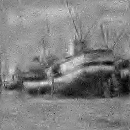
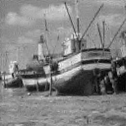
Original image	Random Bernoulli	Multilevel Hadamard	Multilevel Fourier
	Err = 15.7%	Err = 9.6%	Err 8.7%

Figure 6: 12.5% subsampling at $256\!\times\!256$ resolution using DB4 wavelets and various different measurements.

6.1 Universality and RIP or structure?

Theorem 6.2 explains the success of CS when one is constrained to acquire Fourier measurements. Yet, due primarily to the their high global coherence with wavelets, Fourier measurements are often viewed as suboptimal for CS. If one had complete freedom to choose the measurements, and no physical constraints (such as are always present in MRI, for example), then standard CS intuition would suggest random Gaussian or Bernoulli measurements, since they are universal and satisfy the RIP.

However, in reality such measurements are actually highly suboptimal in the presence of structured sparsity. This is demonstrated in Figure 6, where an image is recovered from $m=8192$ measurements taken either as random Bernoulli or multilevel Hadamard or Fourier. As is evident, the latter gives an error that is almost 50% smaller. The reason for this improvement is that whilst Fourier or Hadamard measurements are highly coherent with wavelets, they are asymptotically incoherent, and this can be exploited through multilevel random subsampling to recover asymptotically sparse wavelet coefficients. Random Gaussian/Bernoulli measurements on the other hand cannot take advantage of this structure since they satisfy an RIP.

This observation is an important consequence of our theory. In conclusion, whenever structured sparsity is present (such is the case in the majority of imaging applications, for example) there are substantial improvements to be gained by designing the measurements according to not just the sparsity, but also the additional structure. For a more comprehensive discussion see [53], see also [15, 62].

7 Proofs

The proofs rely on some key propositions from which one can deduce the main theorems. The main work is to prove these proposition, and that will be done subsequently.

7.1 Key results

Proposition 7.1.

Let $U\in\mathcal{B}(l^{2}(\mathbb{N}))$ and suppose that $\Delta$ and $\Omega=\Omega_{1}\cup\ldots\cup\Omega_{r}$ (where the union is disjoint) are subsets of $\mathbb{N}.$ Let $x_{0}\in\mathcal{H}$ and $z\in\mathrm{ran}(P_{\Omega}U)$ be such that $\|z\|\leq\delta$ for $\delta\geq 0$. Let $M\in\mathbb{N}$ and $y=P_{\Omega}Ux_{0}+z$ and $y_{M}=P_{\Omega}UP_{M}x_{0}+z$. Suppose that $\xi\in\mathcal{H}$ and $\xi_{M}\in\mathcal{H}$ satisfiy

$$\|\xi\|_{l^{1}}=\inf_{\eta\in\mathcal{H}}\{\|\eta\|_{l^{1}}:\|P_{\Omega}U\eta-y\|\leq\delta\}.$$ (7.1)

$$\|\xi_{M}\|_{l^{1}}=\inf_{\eta\in\mathbb{C}^{M}}\{\|\eta\|_{l^{1}}:\|P_{\Omega}UP_{M}\eta-y_{M}\|\leq\delta\}.$$ (7.2)

If there exists a vector $\rho=U^{*}P_{\Omega}w$ such that

1. $\|P_{\Delta}U^{*}\left(q_{1}^{-1}P_{\Omega_{1}}\oplus\ldots\oplus q_{r}^{-1}P_{\Omega_{r}}\right)UP_{\Delta}-I_{\Delta}\|\leq\frac{1}{4}$

2. $\max_{i\in\Delta^{c}}\|\left(q_{1}^{-1/2}P_{\Omega_{1}}\oplus\ldots\oplus q_{r}^{-1/2}P_{\Omega_{r}}\right)Ue_{i}\|\leq\sqrt{\frac{5}{4}}$

3. $\|P_{\Delta}\rho-\mathrm{sgn}(P_{\Delta}x_{0})\|\leq\frac{q}{8}.$

4. $\|P_{\Delta}^{\perp}\rho\|_{l^{\infty}}\leq\frac{1}{2}$

5. $\|w\|\leq L\cdot\sqrt{|\Delta|}$

for some $L>0$ and $0<q_{k}\leq 1$, $k=1,\ldots,r$, then we have that

$$\|\xi-x_{0}\|\leq C\cdot\left(\delta\cdot\left(\frac{1}{\sqrt{q}}+L\sqrt{s}\right)+\|P_{\Delta}^{\perp}x_{0}\|_{l^{1}}\right),$$

for some constant $C$, where $s=|\Delta|$ and $q=\min\{q_{k}\}_{k=1}^{r}$. Also, if (ii) is replaced by

$$\max_{i\in\{1,\ldots,M\}\cap\Delta^{c}}\|\left(q_{1}^{-1/2}P_{\Omega_{1}}\oplus\ldots\oplus q_{r}^{-1/2}P_{\Omega_{r}}\right)Ue_{i}\|\leq\sqrt{\frac{5}{4}}$$

and (iv) is replaced by $\|P_{M}P_{\Delta}^{\perp}\rho\|_{l^{\infty}}\leq\frac{1}{2}$ then

$$\|\xi_{M}-x_{0}\|\leq C\cdot\left(\delta\cdot\left(\frac{1}{\sqrt{q}}+L\sqrt{s}\right)+\|P_{M}P_{\Delta}^{\perp}x_{0}\|_{l^{1}}\right).$$ (7.3)

Proof.

First observe that (i) implies that $(P_{\Delta}U^{*}\left(q_{1}^{-1}P_{\Omega_{1}}\oplus\ldots\oplus q_{r}^{-1}P_{\Omega_{r}}\right)UP_{\Delta}|_{P_{\Delta}(\mathcal{H})})^{-1}$ exists and

$$\|(P_{\Delta}U^{*}\left(q_{1}^{-1}P_{\Omega_{1}}\oplus\ldots\oplus q_{r}^{-1}P_{\Omega_{r}}\right)UP_{\Delta}|_{P_{\Delta}(\mathcal{H})})^{-1}\|\leq\frac{4}{3}.$$ (7.4)

Also, (i) implies that

$$\|\left(q_{1}^{-1/2}P_{\Omega_{1}}\oplus\ldots\oplus q_{r}^{-1/2}P_{\Omega_{r}}\right)UP_{\Delta}\|^{2}=\|P_{\Delta}U^{*}\left(q_{1}^{-1}P_{\Omega_{1}}\oplus\ldots\oplus q_{r}^{-1}P_{\Omega_{r}}\right)UP_{\Delta}\|\leq\frac{5}{4},$$ (7.5)

and

$$\begin{split}&\|P_{\Delta}U^{*}\left(q_{1}^{-1}P_{\Omega_{1}}\oplus\ldots\oplus q_{r}^{-1}P_{\Omega_{r}}\right)\|^{2}=\|\left(q_{1}^{-1}P_{\Omega_{1}}\oplus\ldots\oplus q_{r}^{-1}P_{\Omega_{r}}\right)UP_{\Delta}\|^{2}\\ &=\sup_{\|{\eta}\|=1}\|\left(q_{1}^{-1}P_{\Omega_{1}}\oplus\ldots\oplus q_{r}^{-1}P_{\Omega_{r}}\right)UP_{\Delta}\eta\|^{2}\\ &=\sup_{\|{\eta}\|=1}\sum_{k=1}^{r}\|q_{k}^{-1}P_{\Omega_{k}}UP_{\Delta}\eta\|^{2}\leq\frac{1}{q}\sup_{\|{\eta}\|=1}\sum_{k=1}^{r}q_{k}^{-1}\|P_{\Omega_{k}}UP_{\Delta}\eta\|^{2},\quad\frac{1}{q}=\max_{1\leq k\leq r}\{\frac{1}{q_{k}}\}\\ &=\frac{1}{q}\sup_{\|{\eta}\|=1}\langle P_{\Delta}U^{*}\left(\sum_{k=1}^{r}q_{k}^{-1}P_{\Omega_{k}}\right)UP_{\Delta}\eta,\eta\rangle\leq\frac{1}{q}\|P_{\Delta}U^{*}\left(q_{1}^{-1}P_{\Omega_{1}}\oplus\ldots\oplus q_{r}^{-1}P_{\Omega_{r}}\right)UP_{\Delta}\|.\end{split}$$ (7.6)

Thus, (7.5) and (7.6) imply

$$\|P_{\Delta}U^{*}\left(q_{1}^{-1}P_{\Omega_{1}}\oplus\ldots\oplus q_{r}^{-1}P_{\Omega_{r}}\right)\|\leq\sqrt{\frac{5}{4q}}.$$ (7.7)

Suppose that there exists a vector $\rho$, constructed with $y_{0}=P_{\Delta}x_{0}$, satisfying (iii)-(v). Let $\xi$ be a solution to (7.1) and let $h=\xi-x_{0}$. Let $A_{\Delta}=P_{\Delta}U^{*}\left(q_{1}^{-1}P_{\Omega_{1}}\oplus\ldots\oplus q_{r}^{-1}P_{\Omega_{r}}\right)UP_{\Delta}|_{P_{\Delta}(\mathcal{H})}$. Then, it follows from (ii) and observations (7.4), (7.5), (7.7) that

$$\begin{split}&\|P_{\Delta}h\|=\|A_{\Delta}^{-1}A_{\Delta}P_{\Delta}h\|\\ &\leq\|A_{\Delta}^{-1}\|\|P_{\Delta}U^{*}\left(q_{1}^{-1}P_{\Omega_{1}}\oplus\ldots\oplus q_{r}^{-1}P_{\Omega_{r}}\right)U(I-P_{\Delta}^{\perp})h\|\\ &\leq\frac{4}{3}\|P_{\Delta}U^{*}\left(q_{1}^{-1}P_{\Omega_{1}}\oplus\ldots\oplus q_{r}^{-1}P_{\Omega_{r}}\right)\|\|P_{\Omega}Uh\|\\ &+\frac{4}{3}\max_{i\in\Delta^{c}}\|P_{\Delta}U^{*}\left(q_{1}^{-1}P_{\Omega_{1}}\oplus\ldots\oplus q_{r}^{-1}P_{\Omega_{r}}\right)Ue_{i}\|\|P_{\Delta}^{\perp}h\|_{l^{1}}\\ &\leq\frac{4}{3}\|P_{\Delta}U^{*}\left(q_{1}^{-1}P_{\Omega_{1}}\oplus\ldots\oplus q_{r}^{-1}P_{\Omega_{r}}\right)\|\|P_{\Omega}Uh\|\\ &+\frac{4}{3}{\left\|P_{\Delta}U^{*}\left(q_{1}^{-1/2}P_{\Omega_{1}}\oplus\ldots\oplus q_{r}^{-1/2}\right)\right\|}\max_{i\in\Delta^{c}}{\left\|\left(q_{1}^{-1/2}P_{\Omega_{1}}\oplus\ldots\oplus q_{r}^{-1/2}P_{\Omega_{r}}\right)Ue_{i}\right\|}\|P_{\Delta}^{\perp}h\|_{l^{1}}\\ &\leq\frac{4\sqrt{5}}{3\sqrt{q}}\delta+\frac{5}{3}\|P_{\Delta}^{\perp}h\|_{l^{1}},\end{split}$$ (7.8)

where in the final step we use $\|P_{\Omega}Uh\|\leq\|P_{\Omega}U\zeta-y\|+\|z\|\leq 2\delta$. We will now obtain a bound for $\|P_{\Delta}^{\perp}h\|_{l^{1}}$. First note that

$$\begin{split}\|h+x_{0}\|_{l^{1}}&=\|P_{\Delta}h+P_{\Delta}x_{0}\|_{l^{1}}+\|P_{\Delta}^{\perp}(h+x_{0})\|_{l^{1}}\\ &\geq\mathrm{Re}\,\langle P_{\Delta}h,\mathrm{sgn}(P_{\Delta}x_{0})\rangle+\|P_{\Delta}x_{0}\|_{l^{1}}+\|P_{\Delta}^{\perp}h\|_{l^{1}}-\|P_{\Delta}^{\perp}x_{0}\|_{l^{1}}\\ &\geq\mathrm{Re}\,\langle P_{\Delta}h,\mathrm{sgn}(P_{\Delta}x_{0})\rangle+\|x_{0}\|_{l^{1}}+\|P_{\Delta}^{\perp}h\|_{l^{1}}-2\|P_{\Delta}^{\perp}x_{0}\|_{l^{1}}.\end{split}$$ (7.9)

Since $\|x_{0}\|_{l^{1}}\geq\|h+x_{0}\|_{l^{1}}$, we have that

$$\|P_{\Delta}^{\perp}h\|_{l^{1}}\leq\left|\langle P_{\Delta}h,\mathrm{sgn}(P_{\Delta}x_{0})\rangle\right|+2\|P_{\Delta}^{\perp}x_{0}\|_{l^{1}}.$$ (7.10)

We will use this equation later on in the proof, but before we do that observe that some basic adding and subtracting yields

$$\begin{split}\left|\langle P_{\Delta}h,\mathrm{sgn}(x_{0})\rangle\right|&\leq\left|\langle P_{\Delta}h,\mathrm{sgn}(P_{\Delta}x_{0})-P_{\Delta}\rho\rangle\right|+\left|\langle h,\rho\rangle\right|+\left|\langle P_{\Delta}^{\perp}h,P_{\Delta}^{\perp}\rho\rangle\right|\\ &\leq\|P_{\Delta}h\|\|\mathrm{sgn}(P_{\Delta}x_{0})-P_{\Delta}\rho\|+\left|\langle P_{\Omega}Uh,w\rangle\right|+\|P_{\Delta}^{\perp}h\|_{l^{1}}\|P_{\Delta}^{\perp}\rho\|_{l^{\infty}}\\ &\leq\frac{q}{8}\|P_{\Delta}h\|+2L\delta\sqrt{s}+\frac{1}{2}\|P_{\Delta}^{\perp}h\|_{l^{1}}\\ &\leq\frac{\sqrt{5q}}{6}\delta+\frac{5q}{24}\|P_{\Delta}^{\perp}h\|_{l^{1}}+2L\delta\sqrt{s}+\frac{1}{2}\|P_{\Delta}^{\perp}h\|_{l^{1}}\end{split}$$ (7.11)

where the last inequality utilises (LABEL:eq:err_on_supp) and the penultimate inequality follows from properties (iii), (iv) and (v) of the dual vector $\rho$. Combining this with (7.10) and the fact that $q\leq 1$ gives that

$$\|P_{\Delta}^{\perp}h\|_{l^{1}}\leq\delta\left(\frac{4\sqrt{5q}}{3}+8L\sqrt{s}\right)+8\|P_{\Delta}^{\perp}x_{0}\|_{l^{1}}.$$ (7.12)

Thus, (LABEL:eq:err_on_supp) and (7.12) yields:

$$\begin{split}\|h\|&\leq{\left\|P_{\Delta}h\right\|}+{\left\|P_{\Delta}^{\perp}h\right\|}\leq\frac{8}{3}\|P_{\Delta}^{\perp}h\|_{l^{1}}+\frac{4\sqrt{5}}{3\sqrt{q}}\delta\leq\left(8\sqrt{q}+22L\sqrt{s}+\frac{3}{\sqrt{q}}\right)\cdot\delta+22{\left\|P_{\Delta}^{\perp}x_{0}\right\|}_{l^{1}}.\end{split}$$ (7.13)

The proof of the second part of this proposition follows the proof as outlined above and we omit the details. ∎

The next two propositions give sufficient conditions for Proposition 7.1 to be true. But before we state them we need to define the following.

Definition 7.2.

Let $U$ be an isometry of either $\mathbb{C}^{N\times N}$ or $\mathcal{B}(l^{2}(\mathbb{N}))$. For $\mathbf{N}=(N_{1},\ldots,N_{r})\in\mathbb{N}^{r}$, $\mathbf{M}=(M_{1},\ldots,M_{r})\in\mathbb{N}^{r}$ with $1\leq N_{1}<\ldots<N_{r}$ and $1\leq M_{1}<\ldots<M_{r}$, $\mathbf{s}=(s_{1},\ldots,s_{r})\in\mathbb{N}^{r}$ and $1\leq k\leq r$, let

$$\kappa_{\mathbf{N},\mathbf{M}}(k,l)=\max_{\eta\in\Theta}\|P^{N_{k-1}}_{N_{k}}UP^{M_{l-1}}_{M_{l}}\eta\|_{l^{\infty}}\cdot\sqrt{\mu(P^{N_{k-1}}_{N_{k}}U)}.$$

where

$$\Theta=\{\eta:\|\eta\|_{l^{\infty}}\leq 1,|\mathrm{supp}(P_{M_{l}}^{M_{l-1}}\eta)|=s_{l},\,l=1,\ldots,r-1,\,|\mathrm{supp}(P_{M_{r-1}}^{\perp}\eta)|=s_{r},\},$$

and $N_{0}=M_{0}=0$. We also define

$$\kappa_{\mathbf{N},\mathbf{M}}(k,\infty)=\max_{\eta\in\Theta}\|P^{N_{k-1}}_{N_{k}}UP_{M_{r-1}}^{\perp}\eta\|_{l^{\infty}}\cdot\sqrt{\mu(P^{N_{k-1}}_{N_{k}}U)}.$$

Proposition 7.3.

Let $U\in\mathcal{B}(l^{2}(\mathbb{N}))$ be an isometry and $x\in l^{1}(\mathbb{N})$. Suppose that $\Omega=\Omega_{\mathbf{N},\mathbf{m}}$ is a multilevel sampling scheme, where $\mathbf{N}=(N_{1},\ldots,N_{r})\in\mathbb{N}^{r}$ and $\mathbf{m}=(m_{1},\ldots,m_{r})\in\mathbb{N}^{r}$. Let $(\mathbf{s},\mathbf{M})$, where $\mathbf{M}=(M_{1},\ldots,M_{r})\in\mathbb{N}^{r}$, $M_{1}<\ldots<M_{r}$, and $\mathbf{s}=(s_{1},\ldots,s_{r})\in\mathbb{N}^{r}$, be any pair such that the following holds:

• The parameters $N:=N_{r},$ and $K:=\max_{k=1,\ldots,r}(N_{k}-N_{k-1})/m_{k},$ satisfy the weak balancing property with respect to $U$, $M:=M_{r}$ and $s:=s_{1}+\ldots+s_{r}$;

• for $\epsilon>0$ and $1\leq k\leq r$,

  $$1\gtrsim(\log(s\epsilon^{-1})+1)\cdot\frac{N_{k}-N_{k-1}}{m_{k}}\cdot\left(\sum_{l=1}^{r}\kappa_{\mathbf{N},\mathbf{M}}(k,l)\right)\cdot\log\left(KM\sqrt{s}\right),$$ (7.14)

• $$m_{k}\gtrsim(\log(s\epsilon^{-1})+1)\cdot\hat{m}_{k}\cdot\log\left(KM\sqrt{s}\right),$$ (7.15)

  where $\hat{m}_{k}$ satisfies

  $$1\gtrsim\sum_{k=1}^{r}\left(\frac{N_{k}-N_{k-1}}{\hat{m}_{k}}-1\right)\cdot\mu_{\mathbf{N},\mathbf{M}}(k,l)\cdot\tilde{s}_{k},\qquad\forall\,l=1,\ldots,r,$$

  where $\tilde{s}_{1}+\ldots+\tilde{s}_{r}\leq s_{1}+\ldots+s_{r},$ $\tilde{s}_{k}\leq S_{k}(s_{1},\ldots,s_{r})$ and $S_{k}$ is defined in (4.3).

Then (i)-(v) in Proposition 7.1 follow with probability exceeding $1-\epsilon$, with (ii) replaced by

$$\max_{i\in\{1,\ldots,M\}\cap\Delta^{c}}\|\left(q_{1}^{-1/2}P_{\Omega_{1}}\oplus\ldots\oplus q_{r}^{-1/2}P_{\Omega_{r}}\right)Ue_{i}\|\leq\sqrt{\frac{5}{4}},$$ (7.16)

(iv) replaced by $\|P_{M}P_{\Delta}^{\perp}\rho\|_{l^{\infty}}\leq\frac{1}{2}$ and $L$ in (v) is given by

$$L=C\cdot\sqrt{K}\cdot\left(1+\frac{\sqrt{\log_{2}\left(6\epsilon^{-1}\right)}}{\log_{2}(4KM\sqrt{s})}\right).$$ (7.17)

If $m_{k}=N_{k}-N_{k-1}$ for all $1\leq k\leq r$ then (i)-(v) follow with probability one (with the alterations suggested above).

Proposition 7.4.

Let $U\in\mathcal{B}(l^{2}(\mathbb{N}))$ be an isometry and $x\in l^{1}(\mathbb{N})$. Suppose that $\Omega=\Omega_{\mathbf{N},\mathbf{m}}$ is a multilevel sampling scheme, where $\mathbf{N}=(N_{1},\ldots,N_{r})\in\mathbb{N}^{r}$ and $\mathbf{m}=(m_{1},\ldots,m_{r})\in\mathbb{N}^{r}$. Let $(\mathbf{s},\mathbf{M})$, where $\mathbf{M}=(M_{1},\ldots,M_{r})\in\mathbb{N}^{r}$, $M_{1}<\ldots<M_{r}$, and $\mathbf{s}=(s_{1},\ldots,s_{r})\in\mathbb{N}^{r}$, be any pair such that the following holds:

• The parameters $N$ and $K$ (as in Proposition 7.3) satisfy the strong balancing property with respect to $U$, $M=M_{r}$ and $s:=s_{1}+\ldots+s_{r}$;

• for $\epsilon>0$ and $1\leq k\leq r$,

  $$1\gtrsim(\log(s\epsilon^{-1})+1)\cdot\frac{N_{k}-N_{k-1}}{m_{k}}\cdot\left(\kappa_{\mathbf{N},\mathbf{M}}(k,\infty)+\sum_{l=1}^{r-1}\kappa_{\mathbf{N},\mathbf{M}}(k,l)\right)\cdot\log\left(K\tilde{M}\sqrt{s}\right),$$ (7.18)

• $$m_{k}\gtrsim(\log(s\epsilon^{-1})+1)\cdot\hat{m}_{k}\cdot\log\left(K\tilde{M}\sqrt{s}\right),$$ (7.19)

  where $\tilde{M}=\min\{i\in\mathbb{N}:\|\max_{j\geq i}P_{N}UP_{\{j\}}\|\leq 1/(K32\sqrt{s})\}$, and $\hat{m}_{k}$ is as in Proposition 7.3.

Then (i)-(v) in Proposition 7.1 follow with probability exceeding $1-\epsilon$ with $L$ as in (7.17). If $m_{k}=N_{k}-N_{k-1}$ for all $1\leq k\leq r$ then (i)-(v) follow with probability one.

Lemma 7.5 (Bounds for $\kappa_{\mathbf{N},\mathbf{M}}(k,l)$).

For $k,l=1,\ldots,r$

$$\kappa_{\mathbf{N},\mathbf{M}}(k,l)\leq\min\left\{\mu_{\mathbf{N},\mathbf{M}}(k,l)\cdot s_{l},\,\sqrt{s_{l}\cdot\mu(P^{N_{k-1}}_{N_{k}}U)}\cdot{\left\|P^{N_{k-1}}_{N_{k}}UP^{M_{l-1}}_{M_{l}}\right\|}\right\}.$$ (7.20)

Also, for $k=1,\ldots,r$

$$\kappa_{\mathbf{N},\mathbf{M}}(k,\infty)\leq\min\left\{\mu_{\mathbf{N},\mathbf{M}}(k,\infty)\cdot s_{r},\,\sqrt{s_{r}\cdot\mu(P^{N_{k-1}}_{N_{k}}U)}\cdot{\left\|P^{N_{k-1}}_{N_{k}}UP^{\perp}_{M_{r-1}}\right\|}\right\}.$$ (7.21)

Proof.

For $k,l=1,\ldots,r$

$$\kappa_{\mathbf{N},\mathbf{M}}(k,l) =\max_{\eta\in\Theta}\|P^{N_{k-1}}_{N_{k}}UP^{M_{l-1}}_{M_{l}}\eta\|_{l^{\infty}}\cdot\sqrt{\mu(P^{N_{k-1}}_{N_{k}}U)}$$

$$=\max_{\eta\in\Theta}\max_{N_{k-1}<i\leq N_{k}}\left|\sum_{M_{l-1}<j\leq M_{l}}\eta_{j}u_{ij}\right|\cdot\sqrt{\mu(P^{N_{k-1}}_{N_{k}}U)}$$

$$\leq s_{l}\cdot\sqrt{\mu(P^{N_{k-1}}_{N_{k}}UP^{M_{l-1}}_{M_{l}})}\cdot\sqrt{\mu(P^{N_{k-1}}_{N_{k}}U)}\leq s_{l}\cdot\mu_{\mathbf{N},\mathbf{M}}(k,l)$$

since $|u_{ij}|\leq 1$, and similarly,

$$\kappa_{\mathbf{N},\mathbf{M}}(k,\infty)=\max_{\eta\in\Theta}\|P^{N_{k-1}}_{N_{k}}UP_{M_{r-1}}^{\perp}\eta\|_{l^{\infty}}\cdot\sqrt{\mu(P^{N_{k-1}}_{N_{k}}U)}$$

$$=\max_{\eta\in\Theta}\max_{N_{k-1}<i\leq N_{k}}\left|\sum_{M_{r-1}<j}\eta_{j}u_{ij}\right|\cdot\sqrt{\mu(P^{N_{k-1}}_{N_{k}}U)}\leq s_{r}\cdot\mu_{\mathbf{N},\mathbf{M}}(k,\infty).$$

Finally, it is straightforward to show that for $k,l=1,\ldots,r$,

$$\kappa_{\mathbf{N},\mathbf{M}}(k,l)\leq\sqrt{s_{l}}\cdot{\left\|P^{N_{k-1}}_{N_{k}}UP^{M_{l-1}}_{M_{l}}\right\|}\sqrt{\mu(P^{N_{k-1}}_{N_{k}}U)}$$

and

$$\kappa_{\mathbf{N},\mathbf{M}}(k,\infty)\leq\sqrt{s_{r}}\cdot{\left\|P^{N_{k-1}}_{N_{k}}UP^{\perp}_{M_{r-1}}\right\|}\sqrt{\mu(P^{N_{k-1}}_{N_{k}}U)}.$$

∎

We are now ready to prove the main theorems.

Proof of Theorems 4.1 and 5.2.

It is clear that Theorem 4.1 follows from Theorem 5.2, thus it remains to prove the latter. We will apply Proposition 7.3 to a two-level sampling scheme $\Omega=\Omega_{\mathbf{N},\mathbf{m}}$, where $\mathbf{N}=(N_{1},N_{2})$ and $\mathbf{m}=(m_{1},m_{2})$ with $m_{1}=N_{1}$ and $m_{2}=m$. Also, consider $(\mathbf{s},\mathbf{M})$, where $\mathbf{s}=(M_{1},s_{2})$, $\mathbf{M}=(M_{1},M_{2})$. Thus, if $N_{1},N_{2},m_{1},m_{2}\in\mathbb{N}$ are such that

$$N=N_{2},\quad K=\max\left\{\frac{N_{2}-N_{1}}{m_{2}},\frac{N_{1}}{m_{1}}\right\}$$

satisfy the weak balancing property with respect to $U$, $M=M_{2}$ and $s=M_{1}+s_{2}$, we have that (i) - (v) in Proposition 7.1 follow with probability exceeding $1-s\epsilon$, with (ii) replaced by

$$\max_{i\in\{1,\ldots,M\}\cap\Delta^{c}}\|\left(P_{N_{1}}\oplus\frac{N_{2}-N_{1}}{m_{2}}P_{\Omega_{2}}\right)Ue_{i}\|\leq\sqrt{\frac{5}{4}},$$

(iv) replaced by $\|P_{M}P_{\Delta}^{\perp}\rho\|_{l^{\infty}}\leq\frac{1}{2}$ and $L$ in (v) is given by (7.17), if

$$1\gtrsim(\log(s\epsilon^{-1})+1)\cdot\frac{N-N_{1}}{m_{2}}\cdot(\kappa_{\mathbf{N},\mathbf{M}}(2,1)+\kappa_{\mathbf{N},\mathbf{M}}(2,2))\cdot\log\left(KM\sqrt{s}\right),$$ (7.22)

$$m_{2}\gtrsim(\log(s\epsilon^{-1})+1)\cdot\hat{m}_{2}\cdot\log\left(KM\sqrt{s}\right),$$ (7.23)

where $\hat{m}_{2}$ satisfies $1\gtrsim((N_{2}-N_{1})/\hat{m}_{2}-1)\cdot\mu_{N_{1}}\cdot\tilde{s}_{2},$ and $\tilde{s}_{2}\leq S_{2}$ (recall $S_{2}$ from Definition 4.3). Recall from (7.20) that

$$\kappa_{\mathbf{N},\mathbf{M}}(2,1)\leq\sqrt{s_{1}\cdot\mu_{N_{1}}}\cdot{\left\|P_{N_{1}}^{\perp}UP_{M_{1}}\right\|},\quad\kappa_{\mathbf{N},\mathbf{M}}(2,2)\leq s_{2}\cdot\mu_{N_{1}}.$$

Also, it follows directly from Definition 4.3 that

$$S_{2}\leq\left({\left\|P_{N_{1}}^{\perp}UP_{M_{1}}\right\|}\cdot\sqrt{M_{1}}+\sqrt{s_{2}}\right)^{2}.$$

Thus, provided that ${\left\|P_{N_{1}}^{\perp}UP_{M_{1}}\right\|}\leq\gamma/\sqrt{M_{1}}$ where $\gamma$ is as in (i) of Theorem 5.2, we observe that (iii) of Theorem 5.2 implies (7.22) and (7.23). Thus, the theorem now follows from Proposition 7.1. ∎

Proof of Theorem 4.4 and Theorem 5.3.

It is straightforward that Theorem 4.4 follows from Theorem 5.3. Now, recall from Lemma 7.20 that

$$\kappa_{\mathbf{N},\mathbf{M}}(k,l)\leq s_{l}\cdot\mu_{\mathbf{N},\mathbf{M}}(k,l),\quad\kappa_{\mathbf{N},\mathbf{M}}(k,\infty)\leq s_{r}\cdot\mu_{\mathbf{N},\mathbf{M}}(k,\infty),\qquad k,l=1,\ldots,r.$$

Thus, a direct application of Proposition 7.4 and Proposition 7.1 completes the proof.

∎

It remains now to prove Propositions 7.3 and 7.4. This is the content of the next sections.

7.2 Preliminaries

Before we commence on the rather length proof of these propositions, let us recall one of the monumental results in probability theory that will be of greater use later on.

Theorem 7.6.

(Talagrand [58, 43]) There exists a number $K$ with the following property. Consider $n$ independent random variables $X_{i}$ valued in a measurable space $\Omega$ and let $\mathcal{F}$ be a (countable) class of measurable functions on $\Omega.$ Let $Z$ be the random variable $Z=\sup_{f\in\mathcal{F}}\sum_{i\leq n}f(X_{i})$ and define

$$S=\sup_{f\in\mathcal{F}}\|f\|_{\infty},\qquad V=\sup_{f\in\mathcal{F}}\mathbb{E}\left(\sum_{i\leq n}f(X_{i})^{2}\right).$$

If $\mathbb{E}(f(X_{i}))=0$ for all $f\in\mathcal{F}$ and $i\leq n$, then, for each $t>0$, we have

$$\mathbb{P}(|Z-\mathbb{E}(Z)|\geq t)\leq 3\exp\left(-\frac{1}{K}\frac{t}{S}\log\left(1+\frac{tS}{V+S\mathbb{E}(\overline{Z})}\right)\right),$$

where $\overline{Z}=\sup_{f\in\mathcal{F}}|\sum_{i\leq n}f(X_{i})|$.

Note that this version of Talagrand’s theorem is found in [43, Cor. 7.8]. We next present a theorem and several technical propositions that will serve as the main tools in our proofs of Propositions 7.3 and 7.4. A crucial tool herein is the Bernoulli sampling model. We will use the notation $\{a,\ldots,b\}\supset\Omega\sim\mathrm{Ber}(q)$, where $a<b$ $a,b\in\mathbb{N}$, when $\Omega$ is given by $\Omega=\{k:\delta_{k}=1\}$ and $\{\delta_{k}\}_{k=1}^{N}$ is a sequence of Bernoulli variables with $\mathbb{P}(\delta_{k}=1)=q$.

Definition 7.7.

Let $r\in\mathbb{N}$, $\mathbf{N}=(N_{1},\ldots,N_{r})\in\mathbb{N}^{r}$ with $1\leq N_{1}<\ldots<N_{r}$, $\mathbf{m}=(m_{1},\ldots,m_{r})\in\mathbb{N}^{r}$, with $m_{k}\leq N_{k}-N_{k-1}$, $k=1,\ldots,r$, and suppose that

$$\Omega_{k}\subseteq\{N_{k-1}+1,\ldots,N_{k}\},\quad\Omega_{k}\sim\mathrm{Ber}\left(\frac{m_{k}}{N_{k}-N_{k-1}}\right),\quad k=1,\ldots,r,$$

where $N_{0}=0$. We refer to the set $\Omega=\Omega_{\mathbf{N},\mathbf{m}}:=\Omega_{1}\cup\ldots\cup\Omega_{r}.$ as an $(\mathbf{N},\mathbf{m})$-multilevel Bernoulli sampling scheme.

Theorem 7.8.

Let $U\in\mathcal{B}(l^{2}(\mathbb{N}))$ be an isometry. Suppose that $\Omega=\Omega_{\mathbf{N},\mathbf{m}}$ is a multilevel Bernoulli sampling scheme, where $\mathbf{N}=(N_{1},\ldots,N_{r})\in\mathbb{N}^{r}$ and $\mathbf{m}=(m_{1},\ldots,m_{r})\in\mathbb{N}^{r}$. Consider $(\mathbf{s},\mathbf{M})$, where $\mathbf{M}=(M_{1},\ldots,M_{r})\in\mathbb{N}^{r}$, $M_{1}<\ldots<M_{r}$, and $\mathbf{s}=(s_{1},\ldots,s_{r})\in\mathbb{N}^{r}$, and let

$$\Delta=\Delta_{1}\cup\ldots\cup\Delta_{r},\qquad\Delta_{k}\subset\{M_{k-1}+1,\ldots,M_{k}\},\qquad|\Delta_{k}|=s_{k}$$

where $M_{0}=0$. If $\|P_{M_{r}}U^{*}P_{N_{r}}UP_{M_{r}}-P_{M_{r}}\|\leq 1/8$ then, for $\gamma\in(0,1),$

$$\mathbb{P}(\|P_{\Delta}U^{*}(q_{1}^{-1}P_{\Omega_{1}}\oplus\ldots\oplus q_{r}^{-1}P_{\Omega_{r}})UP_{\Delta}-P_{\Delta}\|\geq 1/4)\leq\gamma,$$ (7.24)

where $q_{k}=m_{k}/(N_{k}-N_{k-1}),$ provided that

$$1\gtrsim\frac{N_{k}-N_{k-1}}{m_{k}}\cdot\left(\sum_{l=1}^{r}\kappa_{\mathbf{N},\mathbf{M}}(k,l)\right)\cdot\left(\log\left(\gamma^{-1}\,s\right)+1\right).$$ (7.25)

In addition, if $q=\min\{q_{k}\}^{r}_{k=1}=1$ then

$$\mathbb{P}(\|P_{\Delta}U^{*}(q_{1}^{-1}P_{\Omega_{1}}\oplus\ldots\oplus q_{r}^{-1}P_{\Omega_{r}})UP_{\Delta}-P_{\Delta}\|\geq 1/4)=0.$$

In proving this theorem we deliberately avoid the use of the Matrix Bernstein inequality [32], as Talagrand’s theorem is more convenient for our infinite-dimensional setting. Before we can prove this theorem, we need the following technical lemma.

Lemma 7.9.

Let $U\in\mathcal{B}(l^{2}(\mathbb{N}))$ with $\|U\|\leq 1$, and consider the setup in Theorem 7.8. Let $N=N_{r}$ and let $\{\delta_{j}\}_{j=1}^{N}$ be independent random Bernoulli variables with $\mathbb{P}(\delta_{j}=1)=\tilde{q}_{j},$ $\tilde{q}_{j}=m_{k}/(N_{k}-N_{k-1})$ and $j\in\{N_{k-1}+1,\ldots,N_{k}\},$ and define $Z=\sum_{j=1}^{N}Z_{j},$ $Z_{j}=\left(\tilde{q}_{j}^{-1}\delta_{j}-1\right)\eta_{j}\otimes\bar{\eta}_{j}$ and $\eta_{j}=P_{\Delta}U^{*}e_{j}.$ Then

$$\mathbb{E}\left(\|Z\|\right)^{2}\leq 48\max\{\log(|\Delta|),1\}\,\max_{1\leq j\leq N}\left\{\tilde{q}_{j}^{-1}\|\eta_{j}\|^{2}\right\},$$

when $\left(\max\{\log(|\Delta|),1\}\right)^{-1}\geq 18\max_{1\leq j\leq N}\left\{\tilde{q}_{j}^{-1}\|\eta_{j}\|^{2}\right\}.$

The proof of this lemma involves essentially reworking an argument due to Rudelson [55], and is similar to arguments given previously in [1] (see also [13]). We include it here for completeness as the setup deviates slightly. We shall also require the following result:

Lemma 7.10.

(Rudelson) Let $\eta_{1},\ldots,\eta_{M}\in\mathbb{C}^{n}$ and let $\varepsilon_{1},\ldots\varepsilon_{M}$ be independent Bernoulli variables taking values $1,-1$ with probability $1/2$. Then

$$\mathbb{E}\left(\left\|\sum_{i=1}^{M}\varepsilon_{i}\bar{\eta}_{i}\otimes\eta_{i}\right\|\right)\leq\frac{3}{2}\sqrt{p}\max_{i\leq M}\|\eta_{i}\|\sqrt{\left\|\sum_{i=1}^{M}\bar{\eta}_{i}\otimes\eta_{i}\right\|},$$

where $p=\max\{2,2\log(n)\}$.

Lemma 7.10 is often referred to as Rudelson’s Lemma [55]. However, we use the above complex version that was proven by Tropp [59, Lem. 22].

Proof of Lemma 7.9.

We commence by letting $\tilde{\delta}=\{\tilde{\delta}_{j}\}_{j=1}^{N}$ be independent copies of $\delta=\{\delta_{j}\}_{j=1}^{N}.$ Then, since $\mathbb{E}(Z)=0$,

$$\begin{split}\mathbb{E}_{\delta}\left(\|Z\|\right)&=\mathbb{E}_{\delta}\left(\left\|Z-\mathbb{E}_{\tilde{\delta}}\left(\sum_{j=1}^{N}\left(\tilde{q}_{j}^{-1}\tilde{\delta}_{j}-1\right)\eta_{j}\otimes\bar{\eta}_{j}\right)\right\|\right)\\ &\leq\mathbb{E}_{\delta}\left(\mathbb{E}_{\tilde{\delta}}\left(\left\|Z-\sum_{j=1}^{N}\left(\tilde{q}_{j}^{-1}\tilde{\delta}_{j}-1\right)\eta_{j}\otimes\bar{\eta}_{j}\right\|\right)\right),\end{split}$$ (7.26)

by Jensen’s inequality. Let $\varepsilon=\{\varepsilon_{j}\}_{j=1}^{N}$ be a sequence of Bernoulli variables taking values $\pm 1$ with probability $1/2$. Then, by (7.26), symmetry, Fubini’s Theorem and the triangle inequality, it follows that

$$\begin{split}&\mathbb{E}_{\delta}\left(\|Z\|\right)\leq\mathbb{E}_{\varepsilon}\left(\mathbb{E}_{\delta}\left(\mathbb{E}_{\tilde{\delta}}\left(\left\|\sum_{j=1}^{N}\varepsilon_{j}\left(\tilde{q}_{j}^{-1}\delta_{j}-\tilde{q}_{j}^{-1}\tilde{\delta}_{j}\right)\eta_{j}\otimes\bar{\eta}_{j}\right\|\right)\right)\right)\\ &\quad\leq 2\mathbb{E}_{\delta}\left(\mathbb{E}_{\varepsilon}\left(\left\|\sum_{j=1}^{N}\varepsilon_{j}\tilde{q}_{j}^{-1}\delta_{j}\eta_{j}\otimes\bar{\eta}_{j}\right\|\right)\right).\end{split}$$ (7.27)

We are now able to apply Rudelson’s Lemma (Lemma 7.10). However, as specified before, it is the complex version that is crucial here. By Lemma 7.10 we get that

$$\mathbb{E}_{\varepsilon}\left(\left\|\sum_{j=1}^{N}\varepsilon_{j}\tilde{q}_{j}^{-1}\delta_{j}\eta_{j}\otimes\bar{\eta}_{j}\right\|\right)\leq\frac{3}{2}\sqrt{\max\{2\log(s),2\}}\max_{1\leq j\leq N}\tilde{q}_{j}^{-1/2}\|\eta_{j}\|\sqrt{\left\|\sum_{j=1}^{N}q_{j}^{-1}\tilde{q}_{j}^{-1}\delta_{j}\eta_{j}\otimes\bar{\eta}_{j}\right\|},$$ (7.28)

where $s=|\Delta|$. And hence, by using (7.27) and (7.28), it follows that

$$\mathbb{E}_{\delta}\left(\|Z\|\right)\leq 3\sqrt{\max\{2\log(s),2\}}\max_{1\leq j\leq N}\tilde{q}_{j}^{-1/2}\|\eta_{j}\|\sqrt{\mathbb{E}_{\delta}\left(\left\|Z+\sum_{j=1}^{N}\eta_{j}\otimes\bar{\eta}_{j}\right\|\right)}.$$

Note that $\|\sum_{j=1}^{N}\eta_{j}\otimes\bar{\eta}_{j}\|\leq 1$, since $U$ is an isometry. The result now follows from the straightforward calculus fact that if $r>0$, $c\leq 1$ and $r\leq c\sqrt{r+1}$ then we have that $r\leq c(1+\sqrt{5})/2$. ∎

Proof of Theorem 7.8.

Let $N=N_{r}$ just to be clear here. Let $\{\delta_{j}\}_{j=1}^{N}$ be random Bernoulli variables as defined in Lemma 7.9 and define $Z=\sum_{j=1}^{N}Z_{j},$ $Z_{j}=\left(\tilde{q}_{j}^{-1}\delta_{j}-1\right)\eta_{j}\otimes\bar{\eta}_{j}$ with $\eta_{j}=P_{\Delta}U^{*}e_{j}.$ Now observe that

$$P_{\Delta}U^{*}(q_{1}^{-1}P_{\Omega_{1}}\oplus\ldots\oplus q_{r}^{-1}P_{\Omega_{r}})UP_{\Delta}=\sum_{j=1}^{N}\tilde{q}_{j}^{-1}\delta_{j}\eta_{j}\otimes\bar{\eta}_{j},\quad P_{\Delta}U^{*}P_{N}UP_{\Delta}=\sum_{j=1}^{N}\eta_{j}\otimes\bar{\eta}_{j}.$$ (7.29)

Thus, it follows that

$$\begin{split}\|P_{\Delta}U^{*}(q_{1}^{-1}P_{\Omega_{1}}\oplus\ldots\oplus q_{r}^{-1}P_{\Omega_{r}})UP_{\Delta}-P_{\Delta}\|&\leq\|Z\|+\left\|(P_{\Delta}U^{*}P_{N}UP_{\Delta}-P_{\Delta})\right\|\leq\|Z\|+\frac{1}{8},\end{split}$$ (7.30)

by the assumption that $\|P_{M_{r}}U^{*}P_{N_{r}}UP_{M_{r}}-P_{M_{r}}\|\leq 1/8$. Thus, to prove the assertion we need to estimate $\|Z\|$, and Talagrand’s Theorem (Theorem 7.6) will be our main tool. Note that clearly, since $Z$ is self-adjoint, we have that $\|Z\|=\sup_{\zeta\in\mathcal{G}}|\langle Z\zeta,\zeta\rangle|,$ where $\mathcal{G}$ is a countable set of vectors in the unit ball of $P_{\Delta}(\mathcal{H})$ . For $\zeta\in\mathcal{G}$ define the mappings

$$\hat{\zeta}_{1}(T)=\langle T\zeta,\zeta\rangle,\quad\hat{\zeta}_{2}(T)=-\langle T\zeta,\zeta\rangle,\qquad T\in\mathcal{B}(\mathcal{H}).$$

In order to use Talagrand’s Theorem 7.6 we restrict the domain $\mathcal{D}$ of the mappings $\zeta_{i}$ to

$$\mathcal{D}=\{T\in\mathcal{B}(\mathcal{H}):\|T\|\leq\max_{1\leq j\leq N}\{\tilde{q}^{-1}_{j}\|\eta_{j}\|^{2}\}\}.$$

Let $\mathcal{F}$ denote the family of mappings $\hat{\zeta}_{1},\hat{\zeta}_{2}$ for $\zeta\in\mathcal{G}$. Then $\|Z\|=\sup_{\hat{\zeta}\in\mathcal{F}}\hat{\zeta}(Z)$, and for $i=1,2$ we have

$$|\hat{\zeta}_{i}(Z_{j})|=\left|\left(\tilde{q}^{-1}_{j}\delta_{j}-1\right)\right||\langle\left(\eta_{j}\otimes\bar{\eta}_{j}\right)\zeta,\zeta\rangle|\leq\max_{1\leq j\leq N}\{\tilde{q}^{-1}_{j}\|\eta_{j}\|^{2}\}.$$

Thus, $Z_{j}\in\mathcal{D}$ for $1\leq j\leq N$ and $S:=\sup_{\zeta\in\mathcal{F}}\|\hat{\zeta}\|_{\infty}=\max_{1\leq j\leq N}\{\tilde{q}^{-1}_{j}\|\eta_{j}\|^{2}\}.$ Note that

$$\|\eta_{j}\|^{2}=\langle P_{\Delta}U^{*}e_{j},P_{\Delta}U^{*}e_{j}\rangle=\sum_{k=1}^{r}\langle P_{\Delta_{k}}U^{*}e_{j},P_{\Delta_{k}}U^{*}e_{j}\rangle.$$

Also, note that an easy application of Holder’s inequality gives the following (note that the $l^{1}$ and $l^{\infty}$ bounds are finite because all the projections have finite rank),

$$\begin{split}&|\langle P_{\Delta_{k}}U^{*}e_{j},P_{\Delta_{k}}U^{*}e_{j}\rangle|\leq\|P_{\Delta_{k}}U^{*}e_{j}\|_{l^{1}}\|P_{\Delta_{k}}U^{*}e_{j}\|_{l^{\infty}}\\ &\leq\|P_{\Delta_{k}}U^{*}P_{N_{l}}^{N_{l-1}}\|_{l^{1}\rightarrow l^{1}}\|P_{\Delta_{k}}U^{*}e_{j}\|_{l^{\infty}}\leq\|P_{N_{l}}^{N_{l-1}}UP_{\Delta_{k}}\|_{l^{\infty}\rightarrow l^{\infty}}\cdot\sqrt{\mu(P_{N_{l}}^{N_{l-1}}U)}\leq\kappa_{\mathbf{N},\mathbf{M}}(l,k),\end{split}$$

for $j\in\{N_{l-1}+1,\ldots,N_{l}\}$ and $l\in\{1,\ldots,r\}$. Hence, it follows that

$$\|\eta_{j}\|^{2}\leq\max_{1\leq k\leq r}(\kappa_{\mathbf{N},\mathbf{M}}(k,1)+\ldots+\kappa_{\mathbf{N},\mathbf{M}}(k,r)),$$ (7.31)

and therefore $S\leq\max_{1\leq k\leq r}\left(q_{k}^{-1}\sum_{j=1}^{r}\kappa_{\mathbf{N},\mathbf{M}}(k,j)\right).$ Finally, note that by (7.31) and the reasoning above, it follows that

$$\begin{split}V&:=\sup_{\hat{\zeta}_{i}\in\mathcal{F}}\mathbb{E}\left(\sum_{j=1}^{N}\hat{\zeta}_{i}(Z_{j})^{2}\right)=\sup_{\zeta\in\mathcal{G}}\mathbb{E}\left(\sum_{j=1}^{N}\left(\tilde{q}^{-1}_{j}\delta_{j}-1\right)^{2}|\langle P_{\Delta}U^{*}e_{j},\zeta\rangle|^{4}\right)\\ &\leq\max_{1\leq k\leq r}\|\eta_{k}\|^{2}\left(\frac{N_{k}-N_{k-1}}{m_{k}}-1\right)\sup_{\zeta\in\mathcal{G}}\sum_{j=1}^{N}|\langle e_{j},UP_{\Delta}\zeta\rangle|^{2},\\ &\leq\max_{1\leq k\leq r}\frac{N_{k}-N_{k-1}}{m_{k}}\left(\sum_{l=1}^{r}\kappa_{\mathbf{N},\mathbf{M}}(k,l)\right)\sup_{\zeta\in\mathcal{G}}\|U\zeta\|^{2}=\max_{1\leq k\leq r}\frac{N_{k}-N_{k-1}}{m_{k}}\left(\sum_{l=1}^{r}\kappa_{\mathbf{N},\mathbf{M}}(k,l)\right),\end{split}$$ (7.32)

where we used the fact that $U$ is an isometry to deduce that $\|U\|=1$. Also, by Lemma 7.9 and (7.31) , it follows that

$$\mathbb{E}\left(\|Z\|\right)^{2}\leq 48\,\max_{1\leq k\leq r}\frac{N_{k}-N_{k-1}}{m_{k}}\left(\sum_{l=1}^{r}\kappa_{\mathbf{N},\mathbf{M}}(k,l)\right)\cdot\log(s)$$ (7.33)

when

$$1\geq 18\max_{1\leq k\leq r}\frac{N_{k}-N_{k-1}}{m_{k}}\left(\sum_{l=1}^{r}\kappa_{\mathbf{N},\mathbf{M}}(k,l)\right)\cdot\log(s),$$ (7.34)

(recall that we have assumed $s\geq 3$). Thus, by (7.30) and Talagrand’s Theorem 7.6, it follows that

$$\mathbb{P}\left(\|P_{\Delta}U^{*}(q_{1}^{-1}P_{\Omega_{1}}\oplus\ldots\oplus q_{r}^{-1}P_{\Omega_{r}})UP_{\Delta}-P_{\Delta}\|\geq 1/4\right)$$

$$\leq\mathbb{P}\left(\|Z\|\geq\frac{1}{16}+\sqrt{24\,\max_{1\leq k\leq r}\frac{N_{k}-N_{k-1}}{m_{k}}\left(\sum_{l=1}^{r}\kappa_{\mathbf{N},\mathbf{M}}(k,l)\right)\cdot\log(s)}\right)$$

$$\leq 3\exp\left(-\frac{1}{16K}\left(\max_{1\leq k\leq r}\frac{N_{k}-N_{k-1}}{m_{k}}\left(\sum_{l=1}^{r}\kappa_{\mathbf{N},\mathbf{M}}(k,l)\right)\right)^{-1}\log\left(1+1/32\right)\right),$$ (7.35)

when $m_{k}$’s are chosen such that the right hand side of (7.33) is less than or equal to $1$. Thus, by (7.30) and Talagrand’s Theorem 7.6, it follows that

$$\mathbb{P}\left(\|P_{\Delta}U^{*}(q_{1}^{-1}P_{\Omega_{1}}\oplus\ldots\oplus q_{r}^{-1}P_{\Omega_{r}})UP_{\Delta}-P_{\Delta}\|\geq 1/4\right)$$

$$\leq\mathbb{P}\left(\|Z\|\geq 1/8\right)\leq\mathbb{P}\left(\|Z\|\geq\frac{1}{16}+\mathbb{E}\|Z\|\right)\leq\mathbb{P}\left(\left|\|Z\|-\mathbb{E}\|Z\|\right|\geq\frac{1}{16}\right)$$

$$\leq 3\exp\left(-\frac{1}{16K}\left(\max_{1\leq k\leq r}\frac{N_{k}-N_{k-1}}{m_{k}}\left(\sum_{l=1}^{r}\kappa_{\mathbf{N},\mathbf{M}}(k,l)\right)\right)^{-1}\log\left(1+1/32\right)\right),$$ (7.36)

when $m_{k}$’s are chosen such that the right hand side of (7.33) is less than or equal to $1/16^{2}$. Note that this condition is implied by the assumptions of the theorem as is (7.34). This yields the first part of the theorem. The second claim of this theorem follows from the assumption that $\|P_{M_{r}}U^{*}P_{N_{r}}UP_{M_{r}}-P_{M_{r}}\|\leq 1/8.$ ∎

Proposition 7.11.

Let $U\in\mathcal{B}(l^{2}(\mathbb{N}))$ be an isometry. Suppose that $\Omega=\Omega_{\mathbf{N},\mathbf{m}}$ is a multilevel Bernoulli sampling scheme, where $\mathbf{N}=(N_{1},\ldots,N_{r})\in\mathbb{N}^{r}$ and $\mathbf{m}=(m_{1},\ldots,m_{r})\in\mathbb{N}^{r}$. Consider $(\mathbf{s},\mathbf{M})$, where $\mathbf{M}=(M_{1},\ldots,M_{r})\in\mathbb{N}^{r}$, $M_{1}<\ldots<M_{r}$, and $\mathbf{s}=(s_{1},\ldots,s_{r})\in\mathbb{N}^{r}$, and let $\Delta=\Delta_{1}\cup\ldots\cup\Delta_{r},$ $\Delta_{k}\subset\{M_{k-1},\ldots,M_{k}\},$ $|\Delta_{k}|=s_{k},$ where $M_{0}=0$. Let $\beta\geq 1/4$.

1. If

   $$N:=N_{r},\quad K:=\max_{k=1,\ldots,r}\left\{\frac{N_{k}-N_{k-1}}{m_{k}}\right\},$$

   satisfy the weak balancing property with respect to $U$, $M:=M_{r}$ and $s:=s_{1}+\ldots+s_{r}$, then, for $\xi\in\mathcal{H}$ and $\beta,\gamma>0$, we have that

   $$\mathbb{P}\left(\|P_{M}P_{\Delta}^{\perp}U^{*}(q_{1}^{-1}P_{\Omega_{1}}\oplus\ldots\oplus q_{r}^{-1}P_{\Omega_{r}})UP_{\Delta}\xi\|_{l^{\infty}}>\beta\|\xi\|_{l^{\infty}}\right)\leq\gamma,$$ (7.37)

   provided that

   $$\frac{\beta}{\log\left(\frac{4}{\gamma}(M-s)\right)}\geq C\ \Lambda,\qquad\frac{\beta^{2}}{\log\left(\frac{4}{\gamma}(M-s)\right)}\geq C\ \Upsilon,$$ (7.38)

   for some constant $C>0$, where $q_{k}=m_{k}/(N_{k}-N_{k-1})$ for $k=1,\ldots,r$,

   $$\Lambda=\max_{1\leq k\leq r}\left\{\frac{N_{k}-N_{k-1}}{m_{k}}\cdot\left(\sum_{l=1}^{r}\kappa_{\mathbf{N},\mathbf{M}}(k,l)\right)\right\},$$ (7.39)

   $$\Upsilon=\max_{1\leq l\leq r}\sum_{k=1}^{r}\left(\frac{N_{k}-N_{k-1}}{m_{k}}-1\right)\cdot\mu_{\mathbf{N},\mathbf{M}}(k,l)\cdot\tilde{s}_{k},$$ (7.40)

   for all $\{\tilde{s}_{k}\}_{k=1}^{r}$ such that $\tilde{s}_{1}+\ldots+\tilde{s}_{r}\leq s_{1}+\ldots+s_{r}$ and $\tilde{s}_{k}\leq S_{k}(s_{1},\ldots,s_{r}).$ Moreover, if $q_{k}=1$ for all $k=1,\ldots,r$, then (7.38) is trivially satisfied for any $\gamma>0$ and the left-hand side of (7.37) is equal to zero.

2. If $N$ satisfies the strong Balancing Property with respect to $U,$ $M$ and $s$, then, for $\xi\in\mathcal{H}$ and $\beta,\gamma>0$, we have that

   $$\mathbb{P}\left(\|P_{\Delta}^{\perp}U^{*}(q_{1}^{-1}P_{\Omega_{1}}\oplus\ldots\oplus q_{r}^{-1}P_{\Omega_{r}})UP_{\Delta}\xi\|_{l^{\infty}}>\beta\|\xi\|_{l^{\infty}}\right)\leq\gamma,$$ (7.41)

   provided that

   $$\frac{\beta}{\log\left(\frac{4}{\gamma}(\tilde{\theta}-s)\right)}\geq C\ \Lambda,\qquad\frac{\beta^{2}}{\log\left(\frac{4}{\gamma}(\tilde{\theta}-s)\right)}\geq C\ \Upsilon,$$ (7.42)

   for some constant $C>0$, $\tilde{\theta}=\tilde{\theta}(\{q_{k}\}_{k=1}^{r},1/8,\{N_{k}\}_{k=1}^{r},s,M)$ and $\Upsilon$, $\Lambda$ as defined in (i) and

   $$\tilde{\theta}(\{q_{k}\}_{k=1}^{r},t,\{N_{k}\}_{k=1}^{r},s,M)$$

   $$=\left|\left\{i\in\mathbb{N}:\max_{\begin{subarray}{c}\Gamma_{1}\subset\{1,\ldots,M\},\quad\left|\Gamma_{1}\right|=s\\ \Gamma_{2,j}\subset\{N_{j-1}+1,\ldots,N_{j}\},\quad j=1,\ldots,r\end{subarray}}\|P_{\Gamma_{1}}U^{*}(q_{1}^{-1}P_{\Gamma_{2,1}}\oplus\ldots\oplus q_{r}^{-1}P_{\Gamma_{2,r}})Ue_{i}\|>\frac{t}{\sqrt{s}}\right\}\right|.$$

   Moreover, if $q_{k}=1$ for all $k=1,\ldots,r$, then (7.42) is trivially satisfied for any $\gamma>0$ and the left-hand side of (7.41) is equal to zero.

Proof.

To prove (i) we note that, without loss of generality, we can assume that $\|\xi\|_{l^{\infty}}=1$. Let $\{\delta_{j}\}_{j=1}^{N}$ be random Bernoulli variables with $\mathbb{P}(\delta_{j}=1)=\tilde{q}_{j}=q_{k},$ for $j\in\{N_{k-1}+1,\ldots,N_{k}\}$ and $1\leq k\leq r.$ A key observation that will be crucial below is that

$$\begin{split}&P_{\Delta}^{\perp}U^{*}(q_{1}^{-1}P_{\Omega_{1}}\oplus\ldots\oplus q_{r}^{-1}P_{\Omega_{r}})UP_{\Delta}\xi=\sum_{j=1}^{N}P_{\Delta}^{\perp}U^{*}\tilde{q}_{j}^{-1}\delta_{j}(e_{j}\otimes e_{j})UP_{\Delta}\xi\\ &\qquad=\sum_{j=1}^{N}P_{\Delta}^{\perp}U^{*}(\tilde{q}_{j}^{-1}\delta_{j}-1)(e_{j}\otimes e_{j})UP_{\Delta}\xi+P_{\Delta}^{\perp}U^{*}P_{N}UP_{\Delta}\xi.\end{split}$$ (7.43)

We will use this equation at the end of the argument, but first we will estimate the size of the individual components of $\sum_{j=1}^{N}P_{\Delta}^{\perp}U^{*}(\tilde{q}_{j}^{-1}\delta_{j}-1)(e_{j}\otimes e_{j})UP_{\Delta}\xi$. To do that define, for $1\leq j\leq N$, the random variables

$$X^{i}_{j}=\langle U^{*}(\tilde{q}_{j}^{-1}\delta_{j}-1)(e_{j}\otimes e_{j})UP_{\Delta}\xi,e_{i}\rangle,\qquad i\in\Delta^{c}.$$

We will show using Bernstein’s inequality that, for each $i\in\Delta^{c}$ and $t>0$,

$$\mathbb{P}\left(\left|\sum_{j=1}^{N}X_{j}^{i}\right|>t\right)\leq 4\exp\left(-\frac{t^{2}/4}{\Upsilon+\Lambda t/3}\right).$$ (7.44)

To prove the claim, we need to estimate $\mathbb{E}\left(|X_{j}^{i}|^{2}\right)$ and $|X_{j}^{i}|$. First note that,

$$\mathbb{E}\left(|X_{j}^{i}|^{2}\right)=(\tilde{q}_{j}^{-1}-1)|\langle e_{j},UP_{\Delta}\xi\rangle|^{2}|\langle e_{j},Ue_{i}\rangle|^{2},$$

and note that $|\langle e_{j},Ue_{i}\rangle|^{2}\leq\mu_{\mathbf{N},\mathbf{M}}(k,l)$ for $j\in\{N_{k-1}+1,\ldots,N_{k}\}$ and $i\in\{M_{l-1}+1,\ldots,M_{l}\}$. Hence

$$\sum_{j=1}^{N}\mathbb{E}\left(|X_{j}^{i}|^{2}\right) \leq\sum^{r}_{k=1}(q^{-1}_{k}-1)\mu_{\mathbf{N},\mathbf{M}}(k,l)\|P^{N_{k-1}}_{N_{k}}UP_{\Delta}\xi\|^{2}$$

$$\leq\sup_{\zeta\in\Theta}\left\{\sum^{r}_{k=1}(q^{-1}_{k}-1)\mu_{\mathbf{N},\mathbf{M}}(k,l)\|P^{N_{k-1}}_{N_{k}}U\zeta\|^{2}\right\},$$

where

$$\Theta=\{\eta:\|\eta\|_{l^{\infty}}\leq 1,|\mathrm{supp}(P_{M_{l}}^{M_{l-1}}\eta)|=s_{l},\,l=1,\ldots,r\}.$$

The supremum in the above bound is attained for some $\tilde{\zeta}\in\Theta$. If $\tilde{s}_{k}=\|P_{N_{k}}^{N_{k-1}}U\tilde{\zeta}\|^{2}$, then we have

$$\sum_{j=1}^{N}\mathbb{E}\left(|X_{j}^{i}|^{2}\right)\leq\sum_{k=1}^{r}(q_{k}^{-1}-1)\mu_{\mathbf{N},\mathbf{M}}(k,l)\tilde{s}_{k}.$$ (7.45)

Note that it is clear from the definition that $s_{k}\leq S_{k}(s_{1},\ldots,s_{r})$ for $1\leq k\leq r$. Also, using the fact that $\|U\|\leq 1$ and the definition of $\Theta$, we note that

$$\tilde{s}_{1}+\ldots+\tilde{s}_{r}=\sum_{k=1}^{r}\|P^{N_{k-1}}_{N_{k}}UP_{\Delta}\zeta\|^{2}\leq\|UP_{\Delta}\zeta\|^{2}=\|\zeta\|^{2}\leq s_{1}+\ldots+s_{r}.$$

To estimate $|X_{j}^{i}|$ we start by observing that, by the triangle inequality, the fact that $\|\xi\|_{l^{\infty}}=1$ and Holder’s inequality, it follows that $|\langle\xi,P_{\Delta}U^{*}e_{j}\rangle|\leq\sum_{k=1}^{r}|\langle P_{M_{k}}^{M_{k-1}}\xi,P_{\Delta}U^{*}e_{j}\rangle|,$ and

$$|\langle P_{M_{k}}^{M_{k-1}}\xi,P_{\Delta}U^{*}e_{j}\rangle|\leq\|P_{N_{l}}^{N_{l-1}}UP_{\Delta_{k}}\|_{l^{\infty}\rightarrow l^{\infty}},\quad j\in\{N_{l-1}+1,\ldots,N_{l}\},\quad l\in\{1,\ldots,r\}.$$

Hence, it follows that for $1\leq j\leq N$ and $i\in\Delta^{c}$,

$$\begin{split}&|X_{j}^{i}|=\tilde{q}_{j}^{-1}|(\delta_{j}-\tilde{q}_{j})||\langle\xi,P_{\Delta}U^{*}e_{j}\rangle||\langle e_{j},Ue_{i}\rangle|,\\ &\leq\max_{1\leq k\leq r}\left\{\frac{N_{k}-N_{k-1}}{m_{k}}\cdot\left(\kappa_{\mathbf{N},\mathbf{M}}(k,1)+\ldots+\kappa_{\mathbf{N},\mathbf{M}}(k,r)\right)\right\}.\end{split}$$ (7.46)

Now, clearly $\mathbb{E}(X^{i}_{j})=0$ for $1\leq j\leq N$ and $i\in\Delta^{c}$. Thus, by applying Bernstein’s inequality to $\mathrm{Re}(X_{j}^{i})$ and $\mathrm{Im}(X_{j}^{i})$ for $j=1,\ldots,N$, via (7.45) and (7.46), the claim (7.44) follows.

Now, by (7.44), (7.43) and the assumed weak Balancing property (wBP), it follows that

$$\begin{split}&\mathbb{P}\left(\|P_{M}P_{\Delta}^{\perp}U^{*}(q_{1}^{-1}P_{\Omega_{1}}\oplus\ldots\oplus q_{r}^{-1}P_{\Omega_{r}})UP_{\Delta}\xi\|_{l^{\infty}}>\beta\right)\\ &\leq\sum_{i\in\Delta^{c}\cap\{1,\ldots,M\}}\mathbb{P}\left(\left|\sum_{j=1}^{N}X_{j}^{i}+\langle P_{M}P_{\Delta}^{\perp}U^{*}P_{N}^{\perp}UP_{\Delta}\xi,e_{i}\rangle\right|>\beta\right)\\ &\leq\sum_{i\in\Delta^{c}\cap\{1,\ldots,M\}}\mathbb{P}\left(\left|\sum_{j=1}^{N}X_{j}^{i}\right|>\beta-\|P_{M}P_{\Delta}^{\perp}U^{*}P_{N}UP_{\Delta}\|_{l^{\infty}}\right)\\ &\leq 4(M-s)\exp\left(-\frac{t^{2}/4}{\Upsilon+\Lambda t/3}\right),\quad t=\frac{1}{2}\beta,\qquad\text{by}\,(\ref{claim_Bernstein}),(\text{wBP}),\end{split}$$

Also,

$$4(M-s)\exp\left(-\frac{t^{2}/4}{\Upsilon+\Lambda t/3}\right)\leq\gamma$$

when

$$\log\left(\frac{4}{\gamma}(M-s)\right)^{-1}\geq\left(\frac{4\Upsilon}{t^{2}}+\frac{4\Lambda}{3t}\right).$$

And this concludes the proof of (i). To prove (ii), for $t>0$, suppose that there is a set $\Lambda_{t}\subset\mathbb{N}$ such that

$$\mathbb{P}\left(\sup_{i\in\Lambda_{t}}|\langle P_{\Delta}^{\perp}U^{*}(q_{1}^{-1}P_{\Omega_{1}}\oplus\ldots\oplus q_{r}^{-1}P_{\Omega_{r}})UP_{\Delta}\eta,e_{i}\rangle|>t\right)=0,\qquad|\Lambda_{t}^{c}|<\infty.$$

Then, as before, by (7.44), (7.43) and the assumed strong Balancing property (sBP), it follows that

$$\begin{split}&\mathbb{P}\left(\|P_{\Delta}^{\perp}U^{*}(q_{1}^{-1}P_{\Omega_{1}}\oplus\ldots\oplus q_{r}^{-1}P_{\Omega_{r}})UP_{\Delta}\xi\|_{l^{\infty}}>\beta\right)\\ &\leq\sum_{i\in\Delta^{c}\cap\Lambda_{t}^{c}}\mathbb{P}\left(\left|\sum_{j=1}^{N}X_{j}^{i}+\langle P_{\Delta}^{\perp}U^{*}P_{N}^{\perp}UP_{\Delta}\xi,e_{i}\rangle\right|>\beta\right),\end{split}$$

yielding

$$\begin{split}&\mathbb{P}\left(\|P_{\Delta}^{\perp}U^{*}(q_{1}^{-1}P_{\Omega_{1}}\oplus\ldots\oplus q_{r}^{-1}P_{\Omega_{r}})UP_{\Delta}\xi\|_{l^{\infty}}>\beta\right)\\ &\leq\sum_{i\in\Delta^{c}\cap\Lambda_{t}^{c}}\mathbb{P}\left(\left|\sum_{j=1}^{N}X_{j}^{i}\right|>\beta-\|P_{\Delta}^{\perp}U^{*}P_{N}UP_{\Delta}\|_{l^{\infty}}\right)\\ &\leq 4(\left|\Lambda_{t}^{c}\right|-s)\exp\left(-\frac{t^{2}/4}{\Upsilon+\Lambda t/3}\right)<\gamma,\quad t=\frac{1}{2}\beta,\qquad\text{by}\,(\ref{claim_Bernstein}),(\text{sBP}),\\ \end{split}$$

whenever

$$\log\left(\frac{4}{\gamma}(\left|\Lambda_{t}^{c}\right|-s)\right)^{-1}\geq\left(\frac{4\Upsilon}{t^{2}}+\frac{4\Lambda}{3t}\right).$$

Hence, it remains to obtain a bound on $\left|\Lambda_{t}^{c}\right|$. Let

$$\theta(q_{1},\ldots,q_{r},t,s)=\left\{i\in\mathbb{N}:\max_{\begin{subarray}{c}\Gamma_{1}\subset\{1,\ldots,M\},\quad\left|\Gamma_{1}\right|=s\\ \Gamma_{2,j}\subset\{N_{j-1}+1,\ldots,N_{j}\},\quad j=1,\ldots,r\end{subarray}}\|P_{\Gamma_{1}}U^{*}(q_{1}^{-1}P_{\Gamma_{2,1}}\oplus\ldots\oplus q_{r}^{-1}P_{\Gamma_{2,r}})Ue_{i}\|>\frac{t}{\sqrt{s}}\right\}.$$

Clearly, $\Delta_{t}^{c}\subset\theta(q_{1},\ldots,q_{r},t,s)$ and

$$\|P_{\Gamma_{1}}U^{*}(q_{1}^{-1}P_{\Gamma_{2,1}}\oplus\ldots\oplus q_{r}^{-1}P_{\Gamma_{2,r}})Ue_{i}\| \leq\max_{1\leq j\leq r}q_{j}^{-1}\|P_{N}UP_{i-1}^{\perp}\|\to 0$$

as $i\to\infty$. So, $\left|\theta(q_{1},\ldots,q_{r},t,s)\right|<\infty.$ Furthermore, since $\tilde{\theta}(\{q_{k}\}_{k=1}^{r},t,\{N_{k}\}_{k=1}^{r},s,M)$ is a decreasing function in $t$, for all $t\geq\frac{1}{8}$,

$$\left|\theta(q_{1},\ldots,q_{r},t,s)\right|<\tilde{\theta}(\{q_{k}\}_{k=1}^{r},1/8,\{N_{k}\}_{k=1}^{r},s,M)$$

thus, we have proved (ii). The statements at the end of (i) and (ii) are clear from the reasoning above. ∎

Proposition 7.12.

Consider the same setup as in Proposition 7.11. If $N$ and $K$ satisfy the weak Balancing Property with respect to $U,$ $M$ and $s$, then, for $\xi\in\mathcal{H}$ and $\gamma>0$, we have

$$\begin{split}\mathbb{P}(\|P_{\Delta}U^{*}(q_{1}^{-1}P_{\Omega_{1}}\oplus\ldots\oplus q_{r}^{-1}P_{\Omega_{r}})UP_{\Delta}-P_{\Delta})\xi\|_{l^{\infty}}>\tilde{\alpha}\|\xi\|_{l^{\infty}})\leq\gamma,\end{split}$$ (7.47)

with $\tilde{\alpha}=(2\log_{2}^{1/2}\left(4\sqrt{s}KM\right))^{-1},$ provided that

$$\begin{split}1&\gtrsim\Lambda\cdot\left(\log\left(s\gamma^{-1}\right)+1\right)\cdot\log\left(\sqrt{s}KM\right),\\ 1&\gtrsim\Upsilon\cdot\left(\log\left(s\gamma^{-1}\right)+1\right)\cdot\log\left(\sqrt{s}KM\right),\end{split}$$

where $\Lambda$ and $\Upsilon$ are defined in (7.39) and (7.40). Also,

$$\begin{split}\mathbb{P}(\|P_{\Delta}U^{*}(q_{1}^{-1}P_{\Omega_{1}}\oplus\ldots\oplus q_{r}^{-1}P_{\Omega_{r}})UP_{\Delta}-P_{\Delta})\xi\|_{l^{\infty}}>\frac{1}{2}\|\xi\|_{l^{\infty}})\leq\gamma\end{split}$$ (7.48)

provided that

$$1\gtrsim\Lambda\cdot\left(\log\left(s\gamma^{-1}\right)+1\right),\quad 1\gtrsim\Upsilon\cdot\left(\log\left(s\gamma^{-1}\right)+1\right).$$

Moreover, if $q_{k}=1$ for all $k=1,\ldots,r$, then the left-hand sides of (7.47) and (7.48) are equal to zero.

Proof.

Without loss of generality we may assume that $\|\xi\|_{l^{\infty}}=1.$ Let $\{\delta_{j}\}_{j=1}^{N}$ be random Bernoulli variables with $\mathbb{P}(\delta_{j}=1)=\tilde{q}_{j}:=q_{k},$ with $j\in\{N_{k-1}+1,\ldots,N_{k}\}$ and $1\leq k\leq r$. Let also, for $j\in\mathbb{N},$ $\eta_{j}=(UP_{\Delta})^{*}e_{j}.$ Then, after observing that

$$P_{\Delta}U^{*}(q_{1}^{-1}P_{\Omega_{1}}\oplus\ldots\oplus q_{r}^{-1}P_{\Omega_{r}})UP_{\Delta}=\sum_{j=1}^{N}q_{j}^{-1}\delta_{j}\eta_{j}\otimes\bar{\eta}_{j},\quad P_{\Delta}U^{*}P_{N}UP_{\Delta}=\sum_{j=1}^{N}\eta_{j}\otimes\bar{\eta}_{j},$$

it follows immediately that

$$P_{\Delta}U^{*}(q_{1}^{-1}P_{\Omega_{1}}\oplus\ldots\oplus q_{r}^{-1}P_{\Omega_{r}})UP_{\Delta}-P_{\Delta}=\sum_{j=1}^{N}(\tilde{q}_{j}^{-1}\delta_{j}-1)\eta_{j}\otimes\bar{\eta}_{j}-(P_{\Delta}U^{*}P_{N}UP_{\Delta}-P_{\Delta}).$$ (7.49)

As in the proof of Proposition 7.11 our goal is to eventually use Bernstein’s inequality and the following is therefore a setup for that. Define, for $1\leq j\leq N$, the random variables $Z^{i}_{j}=\langle(\tilde{q}_{j}^{-1}\delta_{j}-1)(\eta_{j}\otimes\bar{\eta}_{j})\xi,e_{i}\rangle,$ for $i\in\Delta.$ We claim that, for $t>0$,

$$\mathbb{P}\left(\left|\sum_{j=1}^{N}Z_{j}^{i}\right|>t\right)\leq 4\exp\left(-\frac{t^{2}/4}{\Upsilon+\Lambda t/3}\right),\qquad i\in\Delta.$$ (7.50)

Now, clearly $\mathbb{E}(Z^{i}_{j})=0$, so we may use Bernstein’s inequality. Thus, we need to estimate $\mathbb{E}\left(|Z_{j}^{i}|^{2}\right)$ and $|Z_{j}^{i}|$. We will start with $\mathbb{E}\left(|Z_{j}^{i}|^{2}\right)$. Note that

$$\mathbb{E}\left(|Z_{j}^{i}|^{2}\right)=(\tilde{q}_{j}^{-1}-1)|\langle e_{j},UP_{\Delta}\xi\rangle|^{2}|\langle e_{j},Ue_{i}\rangle|^{2}.$$ (7.51)

Thus, we can argue exactly as in the proof of Proposition 7.11 and deduce that

$$\sum_{j=1}^{N}\mathbb{E}\left(|Z_{j}^{i}|^{2}\right)\leq\sum_{k=1}^{r}(q_{k}^{-1}-1)\mu_{N_{k-1}}\tilde{s}_{k},$$ (7.52)

where $s_{k}\leq S_{k}(s_{1},\ldots,s_{r})$ for $1\leq k\leq r$ and $\tilde{s}_{1}+\ldots+\tilde{s}_{r}\leq s_{1}+\ldots+s_{r}.$ To estimate $|Z_{j}^{i}|$ we argue as in the proof of Proposition 7.11 and obtain

$$\begin{split}|Z_{j}^{i}|\leq\max_{1\leq k\leq r}\left\{\frac{N_{k}-N_{k-1}}{m_{k}}\cdot(\kappa_{\mathbf{N},\mathbf{M}}(k,1)+\ldots+\kappa_{\mathbf{N},\mathbf{M}}(k,r))\right\}.\end{split}$$ (7.53)

Thus, by applying Bernstein’s inequality to $\mathrm{Re}(Z_{1}^{i}),\ldots,\mathrm{Re}(Z_{N}^{i})$ and $\mathrm{Im}(Z_{1}^{i}),\ldots,\mathrm{Im}(Z_{N}^{i})$ we obtain, via (7.52) and (7.53) the estimate (7.50), and we have proved the claim.

Now armed with (7.50) we can deduce that , by (7.43) and the assumed weak Balancing property (wBP), it follows that

$$\begin{split}&\mathbb{P}\left(\|P_{\Delta}U^{*}(q_{1}^{-1}P_{\Omega_{1}}\oplus\ldots\oplus q_{r}^{-1}P_{\Omega_{r}})UP_{\Delta}-P_{\Delta})\xi\|_{l^{\infty}}>\tilde{\alpha}\right)\\ &\leq\sum_{i\in\Delta}\mathbb{P}\left(\left|\sum_{j=1}^{N}Z_{j}^{i}+\langle(P_{\Delta}U^{*}P_{N}UP_{\Delta}-P_{\Delta})\xi,e_{i}\rangle\right|>\tilde{\alpha}\right)\\ &\leq\sum_{i\in\Delta}\mathbb{P}\left(\left|\sum_{j=1}^{N}Z_{j}^{i}\right|>\tilde{\alpha}-\|P_{M}U^{*}P_{N}UP_{M}-P_{M}\|_{l^{1}}\right),\\ &\leq 4\,s\exp\left(-\frac{t^{2}/4}{\Upsilon+\Lambda t/3}\right),\quad t=\tilde{\alpha},\qquad\text{by}\,(\ref{claim_Bernstein21}),(\text{wBP}).\end{split}$$ (7.54)

Also,

$$4s\exp\left(-\frac{t^{2}/4}{\Upsilon+\Lambda t/3}\right)\leq\gamma,$$ (7.55)

when

$$1\geq\left(\frac{4\Upsilon}{t^{2}}+\frac{4}{3t}\Lambda\right)\cdot\log\left(\frac{4s}{\gamma}\right).$$

And this gives the first part of the proposition. Also, the fact that the left hand side of (7.47) is zero when $q_{k}=1$ for $1\leq k\leq r$ is clear from (7.55). Note that (ii) follows by arguing exactly as above and replacing $\tilde{\alpha}$ by $\frac{1}{4}$.

∎

Proposition 7.13.

Let $U\in\mathcal{B}(l^{2}(\mathbb{N}))$ such that $\|U\|\leq 1$. Suppose that $\Omega=\Omega_{\mathbf{N},\mathbf{m}}$ is a multilevel Bernoulli sampling scheme, where $\mathbf{N}=(N_{1},\ldots,N_{r})\in\mathbb{N}^{r}$ and $\mathbf{m}=(m_{1},\ldots,m_{r})\in\mathbb{N}^{r}$. Consider $(\mathbf{s},\mathbf{M})$, where $\mathbf{M}=(M_{1},\ldots,M_{r})\in\mathbb{N}^{r}$, $M_{1}<\ldots<M_{r}$, and $\mathbf{s}=(s_{1},\ldots,s_{r})\in\mathbb{N}^{r}$, and let $\Delta=\Delta_{1}\cup\ldots\cup\Delta_{r},$ where $\Delta_{k}\subset\{M_{k-1}+1,\ldots,M_{k}\},$ $|\Delta_{k}|=s_{k},$ and $M_{0}=0$. Then, for any $t\in(0,1)$ and $\gamma\in(0,1),$

$$\mathbb{P}\left(\max_{i\in\{1,\ldots,M\}\cap\Delta^{c}}\|P_{\{i\}}U^{*}(q_{1}^{-1}P_{\Omega_{1}}\oplus\ldots\oplus q_{r}^{-1}P_{\Omega_{r}})UP_{\{i\}}\|\geq 1+t\right)\leq\gamma$$

provided that

$$\frac{t^{2}}{4}\geq\log\left(\frac{2M}{\gamma}\right)\cdot\max_{1\leq k\leq r}\left\{\left(\frac{N_{k}-N_{k-1}}{m_{k}}-1\right)\cdot\mu_{\mathbf{N},\mathbf{M}}(k,l)\right\}$$ (7.56)

for all $l=1,\ldots,r$ when $M=M_{r}$ and for all $l=1,\ldots,r-1,\infty$ when $M>M_{r}.$ In addition, if $m_{k}=N_{k}-N_{k-1}$ for each $k=1,\ldots r$, then

$$\mathbb{P}(\|P_{\{i\}}U^{*}(q_{1}^{-1}P_{\Omega_{1}}\oplus\ldots\oplus q_{r}^{-1}P_{\Omega_{r}})UP_{\{i\}}\|\geq 1+t)=0,\quad\forall i\in\mathbb{N}.$$ (7.57)

Proof.

Fix $i\in\{1,\ldots,M\}$. Let $\{\delta_{j}\}_{j=1}^{N}$ be random independent Bernoulli variables with $\mathbb{P}(\delta_{j}=1)=\tilde{q}_{j}:=q_{k}$ for $j\in\{N_{k-1}+1,\ldots,N_{k}\}.$ Define $Z=\sum_{j=1}^{N}Z_{j}$ and $Z_{j}=\left(\tilde{q}_{j}^{-1}\delta_{j}-1\right)\left|u_{ji}\right|^{2}.$ Now observe that

$$P_{\{i\}}U^{*}(q_{1}^{-1}P_{\Omega_{1}}\oplus\ldots\oplus q_{r}^{-1}P_{\Omega_{r}})UP_{\{i\}} =\sum_{j=1}^{N}\tilde{q}_{j}^{-1}\delta_{j}\left|u_{ji}\right|^{2}=\sum_{j=1}^{N}Z_{j}+\sum_{j=1}^{N}\left|u_{ji}\right|^{2},$$

where we interpret $U$ as the infinite matrix $U=\{u_{ij}\}_{i,j\in\mathbb{N}}$. Thus, since $\|U\|\leq 1$,

$$\|P_{\{i\}}U^{*}(q_{1}^{-1}P_{\Omega_{1}}\oplus\ldots\oplus q_{r}^{-1}P_{\Omega_{r}})UP_{\{i\}}\|\leq\left|\sum_{j=1}^{N}Z_{j}\right|+1$$ (7.58)

and it is clear that (7.57) is true. For the case where $q_{k}<1$ for some $k\in\{1,\ldots,r\}$, observe that for $i\in\{M_{l-1}+1,\ldots,M_{l}\}$ (recall that $Z_{j}$ depend on $i$), we have that $\mathbb{E}(Z_{j})=0$. Also,

$$\left|Z_{j}\right|\leq\begin{cases}\max_{1\leq k\leq r}\{\max\{q_{k}^{-1}-1,1\}\cdot\mu_{\mathbf{N},\mathbf{M}}(k,l)\}:=B_{i}&i\in\{M_{l-1}+1,\ldots,M_{l}\}\\ \max_{1\leq k\leq r}\{\max\{q_{k}^{-1}-1,1\}\cdot\mu_{\mathbf{N},\mathbf{M}}(k,\infty)\}:=B_{\infty}&i>M_{r},\end{cases}$$

and, by again using the assumption that $\|U\|\leq 1$,

$$\begin{split}&\sum_{j=1}^{N}\mathbb{E}(\left|Z_{j}\right|^{2})=\sum_{j=1}^{N}(\tilde{q}_{j}^{-1}-1)\left|u_{ji}\right|^{4}\\ &\qquad\quad\leq\begin{cases}\max_{1\leq k\leq r}\{(q_{k}^{-1}-1)\,\mu_{\mathbf{N},\mathbf{M}}(k,l)\}=:\sigma_{i}^{2}&i\in\{M_{l-1}+1,\ldots,M_{l}\}\\ \max_{1\leq k\leq r}\{(q_{k}^{-1}-1)\,\mu_{\mathbf{N},\mathbf{M}}(k,\infty)\}=:\sigma_{\infty}^{2}&i>M_{r}.\end{cases}\end{split}$$

Thus, by Bernstein’s inequality and (7.58),

$$\mathbb{P}(\|P_{\{i\}}U^{*}(q_{1}^{-1}P_{\Omega_{1}}\oplus\ldots\oplus q_{r}^{-1}P_{\Omega_{r}})UP_{\{i\}}\|\geq 1+t)$$

$$\qquad\qquad\qquad\leq\mathbb{P}\left(\left|\sum_{j=1}^{N}Z_{j}\right|\geq t\right)\leq 2\exp\left(-\frac{t^{2}/2}{\sigma^{2}+Bt/3}\right),$$

$$B=\begin{cases}\max_{1\leq i\leq r}B_{i}&M=M_{r},\\ \max_{i\in\{1,\ldots,r-1,\infty\}}B_{i}&M>M_{r}\end{cases},\quad\sigma^{2}=\begin{cases}\max_{1\leq i\leq r}\sigma^{2}_{i}&M=M_{r},\\ \max_{i\in\{1,\ldots,r-1,\infty\}}\sigma^{2}_{1}&M>M_{r}.\end{cases}$$

Applying the union bound yields

$$\mathbb{P}\left(\max_{i\in\{1,\ldots,M\}}\|P_{\{i\}}U^{*}(q_{1}^{-1}P_{\Omega_{1}}\oplus\ldots\oplus q_{r}^{-1}P_{\Omega_{r}})UP_{\{i\}}\|\geq 1+t\right)\leq\gamma$$

whenever (7.56) holds. ∎

7.3 Proofs of Propositions 7.3 and 7.4

The proof of the propositions relies on an idea that originated in a paper by D. Gross [32], namely, the golfing scheme. The variant we are using here is based on an idea from [1] as well as uneven section techniques from [36, 35], see also [31]. However, the informed reader will recognise that the setup here differs substantially from both [32] and [1]. See also [12] for other examples of the use of the golfing scheme. Before we embark on the proof, we will state and prove a useful lemma.

Lemma 7.14.

Let $\tilde{X}_{k}$ be independent binary variables taking values $0$ and $1$, such that $\tilde{X}_{k}=1$ with probability $P$. Then,

$$\mathbb{P}\left(\sum_{i=1}^{N}\tilde{X}_{i}\geq k\right)\geq\left(\frac{N\cdot e}{k}\right)^{-k}\binom{N}{k}P^{k}.$$ (7.59)

Proof.

First observe that

$$\mathbb{P}\left(\sum_{i=1}^{N}\tilde{X}_{i}\geq k\right) =\sum_{i=k}^{N}\binom{N}{i}P^{i}(1-P)^{N-i}=\sum_{i=0}^{N-k}\binom{N}{i+k}P^{i+k}(1-P)^{N-k-i}$$

$$=\binom{N}{k}P^{k}\sum_{i=0}^{N-k}\frac{(N-k)!k!}{(N-i-k)!(i+k)!}P^{i}(1-P)^{N-k-i}$$

$$=\binom{N}{k}P^{k}\sum_{i=0}^{N-k}\binom{N-k}{i}P^{i}(1-P)^{N-k-i}\left[\binom{i+k}{k}\right]^{-1}.$$

The result now follows because $\sum_{i=0}^{N-k}\binom{N-k}{i}P^{i}(1-P)^{N-k-i}=1$ and for $i=0,\ldots,N-k$, we have that

$$\binom{i+k}{k}\leq\left(\frac{(i+k)\cdot e}{k}\right)^{k}\leq\left(\frac{N\cdot e}{k}\right)^{k},$$

where the first inequality follows from Stirling’s approximation (see [17], p. 1186). ∎

Proof of Proposition 7.3.

We start by mentioning that converting from the Bernoulli sampling model and uniform sampling model has become standard in the literature. In particular, one can do this by showing that the Bernoulli model implies (up to a constant) the uniform sampling model in each of the conditions in Proposition 7.1. This is straightforward and the reader may consult [14, 13, 30] for details. We will therefore consider (without loss of generality) only the multilevel Bernoulli sampling scheme.

Recall that we are using the following Bernoulli sampling model: Given $N_{0}=0$, $N_{1},\ldots,N_{r}\in\mathbb{N}$ we let

$$\{N_{k-1}+1,\ldots,N_{k}\}\supset\Omega_{k}\sim\mathrm{Ber}\left(q_{k}\right),\quad q_{k}=\frac{m_{k}}{N_{k}-N_{k-1}}.$$

Note that we may replace this Bernoulli sampling model with the following equivalent sampling model (see [1]):

$$\Omega_{k}=\Omega^{1}_{k}\cup\Omega^{2}_{k}\cup\cdots\cup\Omega^{u}_{k},\qquad\Omega^{j}_{k}\sim\mathrm{Ber}(q^{j}_{k}),\qquad 1\leq k\leq r,$$

for some $u\in\mathbb{N}$ with

$$(1-q^{1}_{k})(1-q^{2}_{k})\cdots(1-q^{u}_{k})=(1-q_{k}).$$ (7.60)

The latter model is the one we will use throughout the proof and the specific value of $u$ will be chosen later. Note also that because of overlaps we will have

$$q^{1}_{k}+q^{2}_{k}+\ldots+q^{u}_{k}\geq q_{k},\qquad 1\leq k\leq r.$$ (7.61)

The strategy of the proof is to show the validity of (i) and (ii), and the existence of a $\rho\in\mathrm{ran}(U^{*}(P_{\Omega_{1}}\oplus\ldots\oplus P_{\Omega_{r}}))$ that satisfies (iii)-(v) in Proposition 7.1 with probability exceeding $1-\epsilon$, where (iii) is replaced by (7.16), (iv) is replaced by $\|P_{M}P_{\Delta}^{\perp}\rho\|_{l^{\infty}}\leq\frac{1}{2}$ and $L$ in (v) is given by (7.17).

Step I: The construction of $\rho$: We start by defining $\gamma=\epsilon/6$ (the reason for this particular choice will become clear later). We also define a number of quantities (and the reason for these choices will become clear later in the proof):

$$u=8\lceil 3v+\log(\gamma^{-1})\rceil,\qquad v=\lceil\log_{2}(8KM\sqrt{s})\rceil,$$ (7.62)

as well as

$$\{q^{i}_{k}:1\leq k\leq r,1\leq i\leq u\},\quad\{\alpha_{i}\}_{i=1}^{u},\quad\{\beta_{i}\}_{i=1}^{u}$$

by

$$q_{k}^{1}=q_{k}^{2}=\frac{1}{4}q_{k},\qquad\tilde{q}_{k}=q_{k}^{3}=\ldots=q_{k}^{u},\qquad q_{k}=(N_{k}-N_{k-1})m_{k}^{-1},\quad 1\leq k\leq r,$$ (7.63)

with

$$(1-q_{k}^{1})(1-q_{k}^{2})\cdots(1-q_{k}^{u})=(1-q_{k})$$

and

$$\alpha_{1}=\alpha_{2}=(2\log_{2}^{1/2}(4KM\sqrt{s}))^{-1},\qquad\alpha_{i}=1/2,\quad 3\leq i\leq u,$$ (7.64)

as well as

$$\beta_{1}=\beta_{2}=\frac{1}{4},\qquad\beta_{i}=\frac{1}{4}\log_{2}(4KM\sqrt{s}),\quad 3\leq i\leq u.$$ (7.65)

Consider now the following construction of $\rho$. We will define recursively the sequences $\{Z_{i}\}_{i=0}^{u}\subset\mathcal{H}$, $\{Y_{i}\}_{i=1}^{u}\subset\mathcal{H}$ and $\{\omega_{i}\}_{i=0}^{u}\subset\mathbb{N}$ as follows: first let $\omega_{0}=\{0\}$, $\omega_{1}=\{0,1\}$ and $\omega_{2}=\{0,1,2\}$. Then define recursively, for $i\geq 3$, the following:

$$\omega_{i}=\begin{cases}\omega_{i-1}\cup\{i\}&\text{if}\,\|(P_{\Delta}-P_{\Delta}U^{*}(\frac{1}{q^{i}_{1}}P_{\Omega^{i}_{1}}\oplus\ldots\oplus\frac{1}{q^{i}_{r}}P_{\Omega^{i}_{r}})UP_{\Delta})Z_{i-1}\|_{l^{\infty}}\leq\alpha_{i}\|P_{\Delta_{k}}Z_{i-1}\|_{l^{\infty}},\\ &\text{and}\,\|P_{M}P_{\Delta}^{\perp}U^{*}(\frac{1}{q^{i}_{1}}P_{\Omega^{i}_{1}}\oplus\ldots\oplus\frac{1}{q^{i}_{r}}P_{\Omega^{i}_{r}})UP_{\Delta}Z_{i-1}\|_{l^{\infty}}\leq\beta_{i}\|Z_{i-1}\|_{l^{\infty}},\\ \omega_{i-1}&\text{otherwise},\end{cases}$$ (7.66)

$$Y_{i}=\begin{cases}\sum_{j\in\omega_{i}}U^{*}(\frac{1}{q^{j}_{1}}P_{\Omega^{j}_{1}}\oplus\ldots\oplus\frac{1}{q^{j}_{r}}P_{\Omega^{j}_{r}})UZ_{j-1}&\text{if}\,i\in\omega_{i},\\ Y_{i-1}&\text{otherwise},\end{cases}\qquad i\geq 1,$$

$$Z_{i}=\begin{cases}\mathrm{sgn}(x_{0})-P_{\Delta}Y_{i}&\text{if}\,i\in\omega_{i},\\ Z_{i-1}&\text{otherwise},\end{cases}\qquad i\geq 1,\qquad Z_{0}=\mathrm{sgn}(x_{0}).$$

Now, let $\{A_{i}\}_{i=1}^{2}$ and $\{B_{i}\}_{i=1}^{5}$ denote the following events

$$\begin{split}&A_{i}:\qquad\|(P_{\Delta}-U^{*}(\frac{1}{q^{i}_{1}}P_{\Omega^{i}_{1}}\oplus\ldots\oplus\frac{1}{q^{i}_{r}}P_{\Omega^{i}_{r}})UP_{\Delta})Z_{i-1}\|_{l^{\infty}}\leq\alpha_{i}\left\|Z_{i-1}\right\|_{l^{\infty}},\qquad i=1,2,\\ &B_{i}:\qquad\|P_{M}P_{\Delta}^{\perp}U^{*}(\frac{1}{q^{i}_{1}}P_{\Omega^{i}_{1}}\oplus\ldots\oplus\frac{1}{q^{i}_{r}}P_{\Omega^{i}_{r}})UP_{\Delta}Z_{i-1}\|_{l^{\infty}}\leq\beta_{i}\|Z_{i-1}\|_{l^{\infty}},\qquad i=1,2,\\ &B_{3}:\qquad\|P_{\Delta}U^{*}(\frac{1}{q_{1}}P_{\Omega_{1}}\oplus\ldots\oplus\frac{1}{q_{r}}P_{\Omega_{r}})UP_{\Delta}-P_{\Delta}\|\leq 1/4,\\ &\qquad\qquad\max_{i\in\Delta^{c}\cap\{1,\ldots,M\}}\|\left(q_{1}^{-1/2}P_{\Omega_{1}}\oplus\ldots\oplus q_{r}^{-1/2}P_{\Omega_{r}}\right)Ue_{i}\|\leq\sqrt{5/4}\\ &B_{4}:\qquad|\omega_{u}|\geq v,\\ &B_{5}:\qquad(\cap_{i=1}^{2}A_{i})\cap(\cap_{i=1}^{4}B_{i}).\end{split}$$ (7.67)

Also, let $\tau(j)$ denote the $j^{\mathrm{th}}$ element in $\omega_{u}$ (e.g. $\tau(0)=0,\tau(1)=1,\tau(2)=2$ etc.) and finally define $\rho$ by

$$\rho=\begin{cases}Y_{\tau(v)}&\text{if $B_{5}$ occurs,}\\ 0&\text{otherwise}.\end{cases}$$

Note that, clearly, $\rho\in\mathrm{ran}(U^{*}P_{\Omega})$, and we just need to show that when the event $B_{5}$ occurs, then (i)-(v) in Proposition 7.1 will follow.

Step II: $B_{5}\Rightarrow(\text{i}),(\text{ii})$. To see that the assertion is true, note that if $B_{5}$ occurs then $B_{3}$ occurs, which immediately (i) and (ii).

Step III: $B_{5}\Rightarrow(\text{iii}),(\text{iv})$. To show the assertion, we start by making the following observations: By the construction of $Z_{\tau(i)}$ and the fact that $Z_{0}=\mathrm{sgn}(x_{0})$, it follows that

$$\begin{split}Z_{\tau(i)}&=Z_{0}-(P_{\Delta}U^{*}(\frac{1}{q^{\tau(1)}_{1}}P_{\Omega^{\tau(1)}_{1}}\oplus\ldots\oplus\frac{1}{q^{\tau(1)}_{r}}P_{\Omega^{\tau(i)}_{r}})UP_{\Delta})Z_{0}\\ &\quad+\ldots+P_{\Delta}U^{*}(\frac{1}{q^{\tau(i)}_{1}}P_{\Omega^{\tau(i)}_{1}}\oplus\ldots\oplus\frac{1}{q^{\tau(i)}_{r}}P_{\Omega^{\tau(i)}_{r}})UP_{\Delta})Z_{\tau(i-1)})\\ &=Z_{\tau(i-1)}-P_{\Delta}U^{*}(\frac{1}{q^{\tau(i)}_{1}}P_{\Omega^{\tau(i)}_{1}}\oplus\ldots\oplus\frac{1}{q^{\tau(i)}_{r}}P_{\Omega^{\tau(i)}_{r}})UP_{\Delta})Z_{\tau(i-1)}\qquad i\leq|\omega_{u}|,\end{split}$$

so we immediately get that

$$Z_{\tau(i)}=(P_{\Delta}-P_{\Delta}U^{*}(\frac{1}{q^{\tau(i)}_{1}}P_{\Omega^{\tau(i)}_{1}}\oplus\ldots\oplus\frac{1}{q^{\tau(i)}_{r}}P_{\Omega^{\tau(i)}_{r}})UP_{\Delta})Z_{\tau(i-1)},\qquad i\leq|\omega_{u}|.$$

Hence, if the event $B_{5}$ occurs, we have, by the choices in (7.64) and (7.65)

$$\|\rho-\mathrm{sgn}(x_{0})\|=\|Z_{\tau(v)}\|\leq\sqrt{s}\|Z_{\tau(v)}\|_{l^{\infty}}\leq\sqrt{s}\prod_{i=1}^{v}\alpha_{\tau(i)}\leq\frac{\sqrt{s}}{2^{v}}\leq\frac{1}{8K},$$ (7.68)

since we have chosen $v=\lceil\log_{2}(8KM\sqrt{s})\rceil$. Also,

$$\begin{split}\|P_{M}P_{\Delta}^{\perp}\rho\|_{l^{\infty}}&\leq\sum_{i=1}^{v}\|P_{M}P_{\Delta}^{\perp}U^{*}(\frac{1}{q^{\tau(i)}_{1}}P_{\Omega^{\tau(i)}_{1}}\oplus\ldots\oplus\frac{1}{q^{\tau(i)}_{r}}P_{\Omega^{\tau(i)}_{r}})UP_{\Delta}Z_{\tau(i-1)}\|_{l^{\infty}}\\ &\leq\sum_{i=1}^{v}\beta_{\tau(i)}\|Z_{\tau(i-1)}\|_{l^{\infty}}\leq\sum_{i=1}^{v}\beta_{\tau(i)}\prod_{j=1}^{i-1}\alpha_{\tau(j)}\\ &\leq\frac{1}{4}(1+\frac{1}{2\log_{2}^{1/2}(a)}+\frac{\log_{2}(a)}{2^{3}\log_{2}(a)}+\ldots+\frac{1}{2^{v-1}})\leq\frac{1}{2},\qquad a=4KM\sqrt{s}.\end{split}$$ (7.69)

In particular, (7.68) and (7.69) imply (iii) and (iv) in Proposition 7.1.

Step IV: $B_{5}\Rightarrow(\text{v})$. To show that, note that we may write the already constructed $\rho$ as $\rho=U^{*}P_{\Omega}w$ where

$$w=\sum_{i=1}^{v}w_{i},\quad w_{i}=\left(\frac{1}{q^{\tau(i)}_{1}}P_{\Omega_{1}}\oplus\ldots\oplus\frac{1}{q^{\tau(i)}_{r}}P_{\Omega_{r}}\right)UP_{\Delta}Z_{\tau(i-1)}.$$

To estimate $\|w\|$ we simply compute

$$\begin{split}\|w_{i}\|^{2}&=\left\langle\left(\frac{1}{q^{\tau(i)}_{1}}P_{\Omega_{1}^{\tau(i)}}\oplus\ldots\oplus\frac{1}{q^{\tau(i)}_{r}}P_{\Omega_{r}^{\tau(i)}}\right)UP_{\Delta}Z_{\tau(i-1)},\left(\frac{1}{q^{\tau(i)}_{1}}P_{\Omega_{1}^{\tau(i)}}\oplus\ldots\oplus\frac{1}{q^{\tau(i)}_{r}}P_{\Omega_{r}^{\tau(i)}}\right)UP_{\Delta}Z_{\tau(i-1)}\right\rangle\\ &=\sum_{k=1}^{r}\left(\frac{1}{q^{\tau(i)}_{k}}\right)^{2}\|P_{\Omega_{k}^{\tau(i)}}UZ_{\tau(i-1)}\|^{2},\end{split}$$

and then use the assumption that the event $B_{5}$ holds to deduce that

$$\begin{split}&\sum_{k=1}^{r}\left(\frac{1}{q^{\tau(i)}_{k}}\right)^{2}\|P_{\Omega_{k}^{\tau(i)}}UZ_{\tau(i-1)}\|^{2}\leq\max_{1\leq k\leq r}\left\{\frac{1}{q^{\tau(i)}_{k}}\right\}\langle\sum_{k=1}^{r}\frac{1}{q^{\tau(i)}_{k}}P_{\Delta}U^{*}P_{\Omega_{k}^{\tau(i)}}UZ_{\tau(i-1)},Z_{\tau(i-1)}\rangle\\ &=\max_{1\leq k\leq r}\left\{\frac{1}{q^{\tau(i)}_{k}}\right\}\langle\left(\sum_{k=1}^{r}\frac{1}{q^{\tau(i)}_{k}}P_{\Delta}U^{*}P_{\Omega_{k}^{\tau(i)}}U-P_{\Delta}\right)Z_{\tau(i-1)},Z_{\tau(i-1)}\rangle+\|Z_{\tau(i-1)}\|^{2}\\ &\leq\max_{1\leq k\leq r}\left\{\frac{1}{q^{\tau(i)}_{k}}\right\}\left(\|Z_{\tau(i-1)}\|\|Z_{\tau(i)}\|+\|Z_{\tau(i-1)}\|^{2}\right)\\ &\leq\max_{1\leq k\leq r}\left\{\frac{1}{q^{\tau(i)}_{k}}\right\}s\left(\|Z_{\tau(i-1)}\|_{l^{\infty}}\|Z_{\tau(i)}\|_{l^{\infty}}+\|Z_{\tau(i-1)}\|_{l^{\infty}}^{2}\right)\leq\max_{1\leq k\leq r}\left\{\frac{1}{q^{\tau(i)}_{k}}\right\}s(\alpha_{i}+1)\left(\prod_{j=1}^{i-1}\alpha_{j}\right)^{2},\end{split}$$

where the last inequality follows from the assumption that the event $B_{5}$ holds. Hence

$$\begin{split}\|w\|\leq\sqrt{s}\sum_{i=1}^{v}\left(\max_{1\leq k\leq r}\left\{\frac{1}{\sqrt{q^{\tau(i)}_{k}}}\right\}\sqrt{\alpha_{i}+1}\prod_{j=1}^{i-1}\alpha_{j}\right)\end{split}$$ (7.70)

Note that, due to the fact that $q_{k}^{1}+\ldots+q_{k}^{u}\geq q_{k}$, we have that

$$\tilde{q}_{k}\geq\frac{m_{k}}{2(N_{k}-N_{k-1})}\frac{1}{8\left\lceil\log(\gamma^{-1})+3\lceil\log_{2}(8KM\sqrt{s})\rceil\right\rceil-2}.$$

This gives, in combination with the chosen values of $\{\alpha_{j}\}$ and (7.70) that

$$\begin{split}\|w\|&\leq 2\sqrt{s}\max_{1\leq k\leq r}\sqrt{\frac{N_{k}-N_{k-1}}{m_{k}}}\left(1+\frac{1}{2\log_{2}^{1/2}\left(4KM\sqrt{s}\right)}\right)^{3/2}\\ &+\sqrt{s}\max_{1\leq k\leq r}\sqrt{\frac{N_{k}-N_{k-1}}{m_{k}}}\cdot\frac{\sqrt{3}}{2}\cdot\frac{\sqrt{8\left\lceil\log(\gamma^{-1})+3\lceil\log_{2}(8KM\sqrt{s})\rceil\right\rceil-2}}{\log_{2}\left(4KM\sqrt{s}\right)}\cdot\sum_{i=3}^{v}\frac{1}{2^{i-3}}\\ &\leq 2\sqrt{s}\max_{1\leq k\leq r}\sqrt{\frac{N_{k}-N_{k-1}}{m_{k}}}\left(\left(\frac{3}{2}\right)^{3/2}+\sqrt{\frac{6}{{\log_{2}(4KM\sqrt{s})}}}\sqrt{1+\frac{\log_{2}\left(\gamma^{-1}\right)+6}{\log_{2}(4KM\sqrt{s})}}\right)\\ &\leq\sqrt{s}\max_{1\leq k\leq r}\sqrt{\frac{N_{k}-N_{k-1}}{m_{k}}}\left(\frac{3\sqrt{3}}{\sqrt{2}}+\frac{2\sqrt{6}}{{\sqrt{\log_{2}(4KM\sqrt{s})}}}\sqrt{1+\frac{\log_{2}\left(\gamma^{-1}\right)+6}{\log_{2}(4KM\sqrt{s})}}\right).\end{split}$$ (7.71)

Step V: The weak balancing property, (7.14) and (7.15) $\Rightarrow\mathbb{P}(A_{1}^{c}\cup A_{2}^{c}\cup B_{1}^{c}\cup B_{2}^{c}\cup B_{3}^{c})\leq 5\gamma$.

To see this, note that by Proposition 7.12 we immediately get (recall that $q^{1}_{k}=q^{2}_{k}=1/4q_{k}$) that $\mathbb{P}(A_{1}^{c})\leq\gamma$ and $\mathbb{P}(A_{2}^{c})\leq\gamma$ as long as the weak balancing property and

$$\begin{split}1&\gtrsim\Lambda\cdot\left(\log\left(s\gamma^{-1}\right)+1\right)\cdot\log\left(\sqrt{s}KM\right),\quad 1\gtrsim\Upsilon\cdot\left(\log\left(s\gamma^{-1}\right)+1\right)\cdot\log\left(\sqrt{s}KM\right),\end{split}$$ (7.72)

are satisfied, where $K=\max_{1\leq k\leq r}(N_{k}-N_{k-1})/m_{k}$,

$$\Lambda=\max_{1\leq k\leq r}\left\{\frac{N_{k}-N_{k-1}}{m_{k}}\cdot\left(\sum_{l=1}^{r}\kappa_{\mathbf{N},\mathbf{M}}(k,l)\right)\right\},$$ (7.73)

$$\Upsilon=\max_{1\leq l\leq r}\sum_{k=1}^{r}\left(\frac{N_{k}-N_{k-1}}{m_{k}}-1\right)\cdot\mu_{\mathbf{N},\mathbf{M}}(k,l)\cdot\tilde{s}_{k},$$ (7.74)

and where $\tilde{s}_{1}+\ldots+\tilde{s}_{r}\leq s_{1}+\ldots+s_{r}$ and $\tilde{s}_{k}\leq S_{k}(s_{1},\ldots,s_{r})$. However, clearly, (7.14) and (7.15) imply (7.72). Also, Proposition 7.11 yields that $\mathbb{P}(B_{1}^{c})\leq\gamma$ and $\mathbb{P}(B_{2}^{c})\leq\gamma$ as long as the weak balancing property and

$$1\gtrsim\Lambda\cdot\log\left(\frac{4}{\gamma}(M-s)\right),\qquad 1\gtrsim\Upsilon\cdot\log\left(\frac{4}{\gamma}(M-s)\right),$$ (7.75)

are satisfied. However, again, (7.14) and (7.15) imply (7.75). Finally, it remains to bound $\mathbb{P}(B_{3}^{c})$. First note that by Theorem 7.8, we may deduce that

$$\mathbb{P}\left(\|P_{\Delta}U^{*}(\frac{1}{q_{1}}P_{\Omega_{1}}\oplus\ldots\oplus\frac{1}{q_{r}}P_{\Omega_{r}})UP_{\Delta}-P_{\Delta}\|>1/4,\right)\leq\gamma/2,$$

when the weak balancing property and

$$1\gtrsim\Lambda\cdot\left(\log\left(\gamma^{-1}\,s\right)+1\right)$$ (7.76)

holds and (7.14) implies (7.76).

For the second part of $B_{3}$, we may deduce from Proposition 7.13 that

$$\mathbb{P}\left(\max_{i\in\Delta^{c}\cap\{1,\ldots,M\}}\|\left(q_{1}^{-1/2}P_{\Omega_{1}}\oplus\ldots\oplus q_{r}^{-1/2}P_{\Omega_{r}}\right)Ue_{i}\|>\sqrt{5/4}\right)\leq\frac{\gamma}{2},$$

whenever

$$1\gtrsim\log\left(\frac{2M}{\gamma}\right)\cdot\max_{1\leq k\leq r}\left\{\left(\frac{N_{k}-N_{k-1}}{m_{k}}-1\right)\cdot\mu_{\mathbf{N},\mathbf{M}}(k,l)\right\},\qquad l=1,\ldots,r.$$ (7.77)

which is true whenever (7.14) holds. Indeed, recalling the definition of $\kappa_{\mathbf{N},\mathbf{M}}(k,j)$ and $\Theta$ in Definition 7.2, observe that

$$\max_{\eta\in\Theta,\|\eta\|_{\infty}=1}\sum_{l=1}^{r}{\left\|P_{N_{k}}^{N_{k-1}}UP_{M_{l}}^{M_{l-1}}\eta\right\|}_{\infty}\geq\max_{\eta\in\Theta,\|\eta\|_{\infty}=1}{\left\|P_{N_{k}}^{N_{k-1}}U\eta\right\|}_{\infty}\geq\sqrt{\mu(P_{N_{k}}^{N_{k-1}}UP_{M_{l}}^{M_{l-1}})}$$ (7.78)

for each $l=1,\ldots,r$ which implies that $\sum_{j=1}^{r}\kappa_{\mathbf{N},\mathbf{M}}(k,j)\geq\mu_{\mathbf{N},\mathbf{M}}(k,l),$ for $l=1,\ldots,r.$ Consequently, (7.77) follows from (7.14). Thus, $\mathbb{P}(B_{3}^{c})\leq\gamma$.

Step VI: The weak balancing property, (7.14) and (7.15) $\Rightarrow\mathbb{P}(B_{4}^{c})\leq\gamma$. To see this, define the random variables $X_{1},\ldots X_{u-2}$ by

$$X_{j}=\begin{cases}0&\omega_{j+2}\neq\omega_{j+1},\\ 1&\omega_{j+2}=\omega_{j+1}.\end{cases}$$ (7.79)

We immediately observe that

$$\mathbb{P}(B_{4}^{c})=\mathbb{P}(|\omega_{u}|<v)=\mathbb{P}(X_{1}+\ldots+X_{u-2}>u-v).$$ (7.80)

However, the random variables $X_{1},\ldots X_{u-2}$ are not independent, and we therefore cannot directly apply the standard Chernoff bound. In particular, we must adapt the setup slightly. Note that

$$\begin{split}&\mathbb{P}(X_{1}+\ldots+X_{u-2}>u-v)\\ &\leq\sum_{l=1}^{\binom{u-2}{u-v}}\mathbb{P}(X_{\pi(l)_{1}}=1,X_{\pi(l)_{2}}=1,\ldots,X_{\pi(l)_{u-v}}=1)\\ &=\sum_{l=1}^{\binom{u-2}{u-v}}\mathbb{P}(X_{\pi(l)_{u-v}}=1\,|\,X_{\pi(l)_{1}}=1,\ldots,X_{\pi(l)_{u-v-1}}=1)\mathbb{P}(X_{\pi(l)_{1}}=1,\ldots,X_{\pi(l)_{u-v-1}}=1)\\ &=\sum_{l=1}^{\binom{u-2}{u-v}}\mathbb{P}(X_{\pi(l)_{u-v}}=1\,|\,X_{\pi(l)_{1}}=1,\ldots,X_{\pi(l)_{u-v-1}}=1)\\ &\qquad\times\mathbb{P}(X_{\pi(l)_{u-v-1}}=1\,|\,X_{\pi(l)_{1}}=1,\ldots,X_{\pi(l)_{u-v-2}}=1)\cdots\mathbb{P}(X_{\pi(l)_{1}}=1)\end{split}$$ (7.81)

where $\pi:\{1,\ldots,\binom{u-2}{u-v}\}\rightarrow\mathbb{N}^{u-v}$ ranges over all $\binom{u-2}{u-v}$ ordered subsets of $\{1,\ldots,u-2\}$ of size $u-v$. Thus, if we can provide a bound $P$ such that

$$\begin{split}P&\geq\mathbb{P}(X_{\pi(l)_{u-v-j}}=1\,|\,X_{\pi(l)_{1}}=1,\ldots,X_{\pi(l)_{u-v-(j+1)}}=1),\\ P&\geq\mathbb{P}(X_{\pi(l)_{1}}=1)\end{split}$$ (7.82)

$$l=1,\ldots,\binom{u-2}{u-v},\quad j=0,\ldots,u-v-2,$$

then, by (7.81),

$$\mathbb{P}(X_{1}+\ldots+X_{u-2}>u-v)\leq\binom{u-2}{u-v}P^{u-v}.$$ (7.83)

We will continue assuming that (7.82) is true, and then return to this inequality below.

Let $\{\tilde{X}_{k}\}_{k=1}^{u-2}$ be independent binary variables taking values $0$ and $1$, such that $\tilde{X}_{k}=1$ with probability $P$. Then, by Lemma 7.14, (7.83) and (7.80) it follows that

$$\mathbb{P}(B_{4}^{c})\leq\mathbb{P}\left(\tilde{X}_{1}+\ldots+\tilde{X}_{u-2}\geq u-v\right)\left(\frac{(u-2)\cdot e}{u-v}\right)^{u-v}.$$ (7.84)

Then, by the standard Chernoff bound ([48, Theorem 2.1, equation 2]), it follows that, for $t>0$,

$$\mathbb{P}\left(\tilde{X}_{1}+\ldots+\tilde{X}_{u-2}\geq(u-2)(t+P)\right)\leq e^{-2(u-2)t^{2}}.$$ (7.85)

Hence, if we let $t=(u-v)/(u-2)-P$, it follows from (7.84) and (7.85) that

$$\mathbb{P}(B_{4}^{c})\leq e^{-2(u-2)t^{2}+(u-v)(\log(\frac{u-2}{u-v})+1)}\leq e^{-2(u-2)t^{2}+u-2}.$$

Thus, by choosing $P=1/4$ we get that $\mathbb{P}(B_{4}^{c})\leq\gamma$ whenever $u\geq x$ and $x$ is the largest root satisfying

$$(x-u)\left(\frac{x-v}{u-2}-\frac{1}{4}\right)-\log(\gamma^{-1/2})-\frac{x-2}{2}=0,$$

and this yields $u\geq 8\lceil 3v+\log(\gamma^{-1/2})\rceil$ which is satisfied by the choice of $u$ in (7.62). Thus, we would have been done with Step VI if we could verify (7.82) with $P=1/4$, and this is the theme in the following claim.

Claim: The weak balancing property, (7.14) and (7.15) $\Rightarrow$ (7.82) with $P=1/4$. To prove the claim we first observe that $X_{j}=0$ when

$$\|(P_{\Delta}-P_{\Delta}U^{*}(\frac{1}{q^{i}_{1}}P_{\Omega^{i}_{1}}\oplus\ldots\oplus\frac{1}{q^{i}_{r}}P_{\Omega^{i}_{r}})UP_{\Delta})Z_{i-1}\|_{l^{\infty}}\leq\frac{1}{2}\|Z_{i-1}\|_{l^{\infty}}$$

$$\|P_{M}P_{\Delta}^{\perp}U^{*}(\frac{1}{q^{i}_{1}}P_{\Omega^{i}_{1}}\oplus\ldots\oplus\frac{1}{q^{i}_{r}}P_{\Omega^{i}_{r}})UP_{\Delta}Z_{i-1}\|_{l^{\infty}}\leq\frac{1}{4}\log_{2}(4KM\sqrt{s})\|Z_{i-1}\|_{l^{\infty}},\qquad i=j+2,$$

where we recall from (7.63) that

$$q_{k}^{3}=q_{k}^{4}=\ldots=q^{u}_{k}=\tilde{q}_{k},\qquad 1\leq k\leq r.$$

Thus, by choosing $\gamma=1/8$ in (7.48) in Proposition 7.12 and $\gamma=1/8$ in (i) in Proposition 7.11, it follows that $\frac{1}{4}\geq\mathbb{P}(X_{j}=1),$ for $j=1,\ldots,u-2,$ when the weak balancing property is satisfied and

$$\left(\log\left(8s\right)+1\right)^{-1} \gtrsim\tilde{q}_{k}^{-1}\cdot\sum_{l=1}^{r}\kappa_{\mathbf{N},\mathbf{M}}(k,l),\quad 1\leq k\leq r$$ (7.86)

$$\left(\log\left(8s\right)+1\right)^{-1} \gtrsim\left(\sum_{k=1}^{r}\left(\tilde{q}_{k}^{-1}-1\right)\cdot\mu_{\mathbf{N},\mathbf{M}}(k,l)\cdot\tilde{s}_{k}\right),\quad 1\leq l\leq r,$$ (7.87)

as well as

$$\frac{\log_{2}(4KM\sqrt{s})}{\log\left(32(M-s)\right)} \gtrsim\tilde{q}_{k}^{-1}\cdot\sum_{l=1}^{r}\kappa_{\mathbf{N},\mathbf{M}}(k,l),\quad 1\leq k\leq r$$ (7.88)

$$\frac{\log_{2}(4KM\sqrt{s})}{\log\left(32(M-s)\right)} \gtrsim\left(\sum_{k=1}^{r}\left(\tilde{q}_{k}^{-1}-1\right)\cdot\mu_{\mathbf{N},\mathbf{M}}(k,l)\cdot\tilde{s}_{k}\right),\quad 1\leq l\leq r,$$ (7.89)

with $K=\max_{1\leq k\leq r}(N_{k}-N_{k-1})/m_{k}.$ Thus, to prove the claim we must demonstrate that (7.14) and (7.15) $\Rightarrow$ (7.86), (7.87), (7.88) and (7.89). We split this into two stages:

Stage 1: (7.15) $\Rightarrow$ (7.89) and (7.87). To show the assertion we must demonstrate that if, for $1\leq k\leq r$,

$$m_{k}\gtrsim(\log(s\epsilon^{-1})+1)\cdot\hat{m}_{k}\cdot\log\left(KM\sqrt{s}\right),$$ (7.90)

where $\hat{m}_{k}$ satisfies

$$1\gtrsim\sum_{k=1}^{r}\left(\frac{N_{k}-N_{k-1}}{\hat{m}_{k}}-1\right)\cdot\mu_{\mathbf{N},\mathbf{M}}(k,l)\cdot\tilde{s}_{k},\qquad l=1,\ldots,r,$$ (7.91)

we get (7.89) and (7.87). To see this, note that by (7.61) we have that

$$q^{1}_{k}+q^{2}_{k}+(u-2)\tilde{q}_{k}\geq q_{k},\qquad 1\leq k\leq r,$$ (7.92)

so since $q^{1}_{k}=q^{2}_{k}=\frac{1}{4}q_{k}$, and by (7.92), (7.90) and the choice of $u$ in (7.62), it follows that

$$2(8(\lceil\log(\gamma^{-1})+ 3\lceil\log_{2}(8KM\sqrt{s})\rceil\rceil)-2)\tilde{q}_{k}\geq q_{k}=\frac{m_{k}}{N_{k}-N_{k-1}}$$

$$\geq C\frac{\hat{m}_{k}}{N_{k}-N_{k-1}}(\log(s\epsilon^{-1})+1)\log\left(KM\sqrt{s}\right)$$

$$\geq C\frac{\hat{m}_{k}}{N_{k}-N_{k-1}}(\log(s)+1)(\log\left(KM\sqrt{s}\right)+\log(\epsilon^{-1})),$$

for some constant $C$ (recall that we have assumed that $\log(s)\geq 1$). And this gives (by recalling that $\gamma=\epsilon/6$) that $\tilde{q}_{k}\geq\hat{C}\frac{\hat{m}_{k}}{N_{k}-N_{k-1}}(\log(s)+1),$ for some constant $\hat{C}$. Thus, (7.15) implies that for $1\leq l\leq r$,

$$1 \gtrsim\left(\log\left(s\right)+1\right)\left(\sum_{k=1}^{r}\left(\frac{N_{k}-N_{k-1}}{m_{k}(\log(s)+1)}-\frac{1}{\log(s)+1}\right)\cdot\mu_{\mathbf{N},\mathbf{M}}(k,l)\cdot\tilde{s}_{k}\right)$$

$$\gtrsim\left(\log\left(s\right)+1\right)\left(\sum_{k=1}^{r}\left(\tilde{q}_{k}^{-1}-1\right)\cdot\mu_{\mathbf{N},\mathbf{M}}(k,l)\cdot\tilde{s}_{k}\right),$$

and this implies (7.89) and (7.87), given an appropriate choice of the constant $C$.

Stage 2: (7.14) $\Rightarrow$ (7.88) and (7.86). To show the assertion we must demonstrate that if, for $1\leq k\leq r$,

$$1\gtrsim(\log(s\epsilon^{-1})+1)\cdot\frac{N_{k}-N_{k-1}}{m_{k}}\cdot(\sum_{l=1}^{r}\kappa_{\mathbf{N},\mathbf{M}}(k,l))\cdot\log\left(KM\sqrt{s}\right),$$ (7.93)

we obtain (7.88) and (7.86). To see this, note that by arguing as above via the fact that $q^{1}_{k}=q^{2}_{k}=\frac{1}{4}q_{k}$, and by (7.92), (7.93) and the choice of $u$ in (7.62) we have that

$$2(8(\lceil\log(\gamma^{-1})+ 3\lceil\log_{2}(8KM\sqrt{s})\rceil\rceil)-2)\tilde{q}_{k}\geq q_{k}=\frac{m_{k}}{N_{k}-N_{k-1}}$$

$$\geq C\cdot(\sum_{l=1}^{r}\kappa_{\mathbf{N},\mathbf{M}}(k,l))\cdot(\log(s\epsilon^{-1})+1)\cdot\log\left(KM\sqrt{s}\right)$$

$$\geq C\cdot(\sum_{l=1}^{r}\kappa_{\mathbf{N},\mathbf{M}}(k,l))\cdot(\log(s)+1)\left(\log(\epsilon^{-1})+\log\left(KM\sqrt{s}\right)\right),$$

for some constant $C$. Thus, we have that for some appropriately chosen constant $\hat{C}$, $\tilde{q}_{k}\geq\hat{C}\cdot(\log(s)+1)\cdot\sum_{l=1}^{r}\kappa_{\mathbf{N},\mathbf{M}}(k,l).$ So, (7.88) and (7.86) holds given an appropriately chosen $C$. This yields the last puzzle of the proof, and we are done. ∎

Proof of Proposition 7.4.

The proof is very close to the proof of Proposition 7.3 and we will simply point out the differences. The strategy of the proof is to show the validity of (i) and (ii), and the existence of a $\rho\in\mathrm{ran}(U^{*}(P_{\Omega_{1}}\oplus\ldots\oplus P_{\Omega_{r}}))$ that satisfies (iii)-(v) in Proposition 7.1 with probability exceeding $1-\epsilon$.

Step I: The construction of $\rho$: The construction is almost identical to the construction in the proof of Proposition 7.3, except that

$$u=8\lceil\log(\gamma^{-1})+3v\rceil,\qquad v=\lceil\log_{2}(8K\tilde{M}\sqrt{s})\rceil,$$ (7.94)

$$\alpha_{1}=\alpha_{2}=(2\log_{2}^{1/2}(4K\tilde{M}\sqrt{s}))^{-1},\qquad\alpha_{i}=1/2,\quad 3\leq i\leq u,$$

as well as

$$\beta_{1}=\beta_{2}=\frac{1}{4},\qquad\beta_{i}=\frac{1}{4}\log_{2}(4K\tilde{M}\sqrt{s}),\quad 3\leq i\leq u,$$

and (7.66) gets changed to

$$\omega_{i}=\begin{cases}\omega_{i-1}\cup\{i\}&\text{if}\,\|(P_{\Delta}-P_{\Delta}U^{*}(\frac{1}{q^{i}_{1}}P_{\Omega^{i}_{1}}\oplus\ldots\oplus\frac{1}{q^{i}_{r}}P_{\Omega^{i}_{r}})UP_{\Delta})Z_{i-1}\|_{l^{\infty}}\leq\alpha_{i}\|P_{\Delta_{k}}Z_{i-1}\|_{l^{\infty}},\\ &\text{and}\,\|P_{\Delta}^{\perp}U^{*}(\frac{1}{q^{i}_{1}}P_{\Omega^{i}_{1}}\oplus\ldots\oplus\frac{1}{q^{i}_{r}}P_{\Omega^{i}_{r}})UP_{\Delta}Z_{i-1}\|_{l^{\infty}}\leq\beta_{i}\|Z_{i-1}\|_{l^{\infty}},\\ \omega_{i-1}&\text{otherwise},\end{cases}$$

the events $B_{i}$, $i=1,2$ in (7.67) get replaced by

$$\begin{split}&\widetilde{B}_{i}:\qquad\|P_{\Delta}^{\perp}U^{*}(\frac{1}{q^{i}_{1}}P_{\Omega^{i}_{1}}\oplus\ldots\oplus\frac{1}{q^{i}_{r}}P_{\Omega^{i}_{r}})UP_{\Delta}Z_{i-1}\|_{l^{\infty}}\leq\beta_{i}\|Z_{i-1}\|_{l^{\infty}},\qquad i=1,2.\\ \end{split}$$

and the second part of $B_{3}$ becomes

$$\max_{i\in\Delta^{c}}\|\left(q_{1}^{-1/2}P_{\Omega_{1}}\oplus\ldots\oplus q_{r}^{-1/2}P_{\Omega_{r}}\right)Ue_{i}\|\leq\sqrt{5/4}.$$

Step II: $B_{5}\Rightarrow(\text{i}),(\text{ii})$. This step is identical to Step II in the proof of Proposition 7.3.

Step III: $B_{5}\Rightarrow(\text{iii}),(\text{iv})$. Equation (7.69) gets changed to

$$\begin{split}\|P_{\Delta}^{\perp}\rho\|_{l^{\infty}}&\leq\sum_{i=1}^{v}\|P_{\Delta}^{\perp}U^{*}(\frac{1}{q^{\tau(i)}_{1}}P_{\Omega^{\tau(i)}_{1}}\oplus\ldots\oplus\frac{1}{q^{\tau(i)}_{r}}P_{\Omega^{\tau(i)}_{r}})UP_{\Delta}Z_{\tau(i-1)}\|_{l^{\infty}}\\ &\leq\sum_{i=1}^{v}\beta_{\tau(i)}\|Z_{\tau(i-1)}\|_{l^{\infty}}\leq\sum_{i=1}^{v}\beta_{\tau(i)}\prod_{j=1}^{i-1}\alpha_{\tau(j)}\\ &\leq\frac{1}{4}(1+\frac{1}{2\log_{2}^{1/2}(a)}+\frac{\log_{2}(a)}{2^{3}\log_{2}(a)}+\ldots+\frac{1}{2^{v-1}})\leq\frac{1}{2},\qquad a=4\tilde{M}K\sqrt{s}.\end{split}$$

Step IV: $B_{5}\Rightarrow(\text{v})$. This step is identical to Step IV in the proof of Proposition 7.3.

Step V: The strong balancing property, (7.18) and (7.19) $\Rightarrow\mathbb{P}(A_{1}^{c}\cup A_{2}^{c}\cup\widetilde{B}_{1}^{c}\cup\widetilde{B}_{2}^{c}\cup B_{3}^{c})\leq 5\gamma$. We will start by bounding $\mathbb{P}(\widetilde{B}_{1}^{c})$ and $\mathbb{P}(\widetilde{B}_{2}^{c}).$ Note that by Proposition 7.11 (ii) it follows that $\mathbb{P}(\widetilde{B}_{1}^{c})\leq\gamma$ and $\mathbb{P}(\widetilde{B}_{2}^{c})\leq\gamma$ as long as the strong balancing property is satisfied and

$$1\gtrsim\Lambda\cdot\log\left(\frac{4}{\gamma}(\tilde{\theta}-s)\right),\qquad 1\gtrsim\Upsilon\cdot\log\left(\frac{4}{\gamma}(\tilde{\theta}-s)\right)$$ (7.95)

where $\tilde{\theta}=\tilde{\theta}(\{q^{i}_{k}\}_{k=1}^{r},1/8,\{N_{k}\}_{k=1}^{r},s,M)$ for $i=1,2$ and where $\tilde{\theta}$ is defined in Proposition 7.11 (ii) and $\Lambda$ and $\Upsilon$ are defined in (7.73) and (7.74). Note that it is easy to see that we have

$$\left|\left\{j\in\mathbb{N}:\max_{\begin{subarray}{c}\Gamma_{1}\subset\{1,\ldots,M\},\quad\left|\Gamma_{1}\right|=s\\ \Gamma_{2,j}\subset\{N_{j-1}+1,\ldots,N_{j}\},\quad j=1,\ldots,r\end{subarray}}\|P_{\Gamma_{1}}U^{*}((q^{i}_{1})^{-1}P_{\Gamma_{2,1}}\oplus\ldots\oplus(q^{i}_{r})^{-1}P_{\Gamma_{2,r}})Ue_{j}\|>\frac{1}{8\sqrt{s}}\right\}\right|\leq\tilde{M},$$

where

$$\tilde{M}=\min\{i\in\mathbb{N}:\max_{j\geq i}\|P_{N}UP_{\{j\}}\|\leq 1/(K32\sqrt{s})\},$$

and this follows from the choice in (7.63) where $q_{k}^{1}=q_{k}^{2}=\frac{1}{4}q_{k}$ for $1\leq k\leq r$. Thus, it immediately follows that (7.18) and (7.19) imply (7.95). To bound $\mathbb{P}(B_{3}^{c})$, we first deduce as in Step V of the proof of Proposition 7.3 that

$$\mathbb{P}\left(\|P_{\Delta}U^{*}(\frac{1}{q_{1}}P_{\Omega_{1}}\oplus\ldots\oplus\frac{1}{q_{r}}P_{\Omega_{r}})UP_{\Delta}-P_{\Delta}\|>1/4,\right)\leq\gamma/2$$

when the strong balancing property and (7.18) holds. For the second part of $B_{3}$, we know from the choice of $\tilde{M}$ that

$$\max_{i\geq\tilde{M}}\|\left(q_{1}^{-1/2}P_{\Omega_{1}}\oplus\ldots\oplus q_{r}^{-1/2}P_{\Omega_{r}}\right)Ue_{i}\|\leq\sqrt{\frac{5}{4}}$$

and we may deduce from Proposition 7.13 that

$$\mathbb{P}\left(\max_{i\in\Delta^{c}\cap\{1,\ldots,\tilde{M}\}}\|\left(q_{1}^{-1/2}P_{\Omega_{1}}\oplus\ldots\oplus q_{r}^{-1/2}P_{\Omega_{r}}\right)Ue_{i}\|>\sqrt{5/4}\right)\leq\frac{\gamma}{2},$$

whenever

$$1\gtrsim\log\left(\frac{2\tilde{M}}{\gamma}\right)\cdot\max_{1\leq k\leq r}\left\{\left(\frac{N_{k}-N_{k-1}}{m_{k}}-1\right)\,\mu_{\mathbf{N},\mathbf{M}}(k,l)\right\},\quad l=1,\ldots,r-1,\infty,$$

which is true whenever (7.18) holds, since by a similar argument to (7.78),

$$\kappa_{\mathbf{N},\mathbf{M}}(k,\infty)+\sum_{j=1}^{r-1}\kappa_{\mathbf{N},\mathbf{M}}(k,j)\geq\mu_{\mathbf{N},\mathbf{M}}(k,l),\qquad l=1,\ldots,r-1,\infty.$$

Thus, $\mathbb{P}(B_{3}^{c})\leq\gamma$. As for bounding $\mathbb{P}(A_{1}^{c})$ and $\mathbb{P}(A_{2}^{c})$, observe that by the strong balancing property $\tilde{M}\geq M$, thus this is done exactly as in Step V of the proof of Proposition 7.3.

Step VI: The strong balancing property, (7.18) and (7.19) $\Rightarrow\mathbb{P}(B_{4}^{c})\leq\gamma$. To see this, define the random variables $X_{1},\ldots X_{u-2}$ as in (7.79). Let $\pi$ be defined as in Step VI of the proof of Proposition 7.3. Then it suffices to show that (7.18) and (7.19) imply that for $l=1,\ldots\binom{u-2}{u-v}$ and $j=0,\ldots,u-v-2$, we have

$$\begin{split}\frac{1}{4}&\geq\mathbb{P}(X_{\pi(l)_{u-v-j}}=1\,|\,X_{\pi(l)_{1}}=1,\ldots,X_{\pi(l)_{u-v-(j+1)}}=1),\\ \frac{1}{4}&\geq\mathbb{P}(X_{\pi(l)_{1}}=1).\end{split}$$ (7.96)

Claim: The strong balancing property, (7.18) and (7.19) $\Rightarrow$ (7.96). To prove the claim we first observe that $X_{j}=0$ when

$$\|(P_{\Delta}-P_{\Delta}U^{*}(\frac{1}{q^{i}_{1}}P_{\Omega^{i}_{1}}\oplus\ldots\oplus\frac{1}{q^{i}_{r}}P_{\Omega^{i}_{r}})UP_{\Delta})Z_{i-1}\|_{l^{\infty}}\leq\frac{1}{2}\|Z_{i-1}\|_{l^{\infty}}$$

$$\|P_{\Delta}^{\perp}U^{*}(\frac{1}{q^{i}_{1}}P_{\Omega^{i}_{1}}\oplus\ldots\oplus\frac{1}{q^{i}_{r}}P_{\Omega^{i}_{r}})UP_{\Delta}Z_{i-1}\|_{l^{\infty}}\leq\frac{1}{4}\log_{2}(4K\tilde{M}\sqrt{s})\|Z_{i-1}\|_{l^{\infty}},\qquad i=j+2.$$

Thus, by again recalling from (7.63) that $q_{k}^{3}=q_{k}^{4}=\ldots=q^{u}_{k}=\tilde{q}_{k},$ $1\leq k\leq r$, and by choosing $\tilde{\gamma}=1/4$ in (7.48) in Proposition 7.12 and $\tilde{\gamma}=1/4$ in (ii) in Proposition 7.11, we conclude that (7.96) follows when the strong balancing property is satisfied as well as (7.86) and (7.87). and

$$\frac{\log_{2}(4K\tilde{M}\sqrt{s})}{\log\left(16(\tilde{M}-s)\right)} \geq C_{2}\cdot\tilde{q}_{k}^{-1}\cdot\left(\sum_{l=1}^{r-1}\kappa_{\mathbf{N},\mathbf{M}}(k,l)+\kappa_{\mathbf{N},\mathbf{M}}(k,\infty)\right),\quad k=1,\ldots,r$$ (7.97)

$$\frac{\log_{2}(4K\tilde{M}\sqrt{s})}{\log\left(16(\tilde{M}-s)\right)} \geq C_{2}\cdot\left(\sum_{l=1}^{r}\left(\tilde{q}_{k}^{-1}-1\right)\cdot\mu_{\mathbf{N},\mathbf{M}}(k,l)\cdot\tilde{s}_{k}\right),\quad l=1,\ldots,r-1,\infty$$ (7.98)

for $K=\max_{1\leq k\leq r}(N_{k}-N_{k-1})/m_{k}.$ for some constants $C_{1}$ and $C_{2}$. Thus, to prove the claim we must demonstrate that (7.18) and (7.19) $\Rightarrow$ (7.86), (7.87), (7.97) and (7.98). This is done by repeating Stage 1 and Stage 2 in Step VI of the proof of Proposition 7.3 almost verbatim, except replacing $M$ by $\tilde{M}$. ∎

7.4 Proof of Theorem 6.2

Throughout this section, we use the notation

$$\hat{f}(\xi)=\int_{\mathbb{R}}f(x)e^{-ix\xi}\mathrm{d}x,$$ (7.99)

to denote the Fourier transform of a function $f\in L^{1}(\mathbb{R})$.

7.4.1 Setup

We first introduce the wavelet sparsity and Fourier sampling bases that we consider, and in particular, their orderings. Consider an orthonormal basis of compactly supported wavelets with an MRA [20, 21]. For simplicity, suppose that $\mathrm{supp}(\Psi)=\mathrm{supp}(\Phi)=[0,a]$ for some $a\geq 1$, where $\Psi$ and $\Phi$ are the mother wavelet and scaling function respectively. For later use, we recall the following three properties of any such wavelet basis:

1. There exist $\alpha\geq 1$, $C_{\Psi}$ and $C_{\Phi}>0$, such that

   $$\left|\hat{\Phi}(\xi)\right|\leq\frac{C_{\Phi}}{(1+\left|\xi\right|)^{\alpha}},\quad\left|\hat{\Psi}(\xi)\right|\leq\frac{C_{\Psi}}{(1+\left|\xi\right|)^{\alpha}}.$$ (7.100)

   See [21, Eqn.  (7.1.4)]. We will denote $\max\{C_{\Psi},C_{\Phi}\}$ by $C_{\Phi,\Psi}$.

2. $\Psi$ has $v\geq 1$ vanishing moments and $\hat{\Psi}(z)=(-iz)^{v}\theta_{\Psi}(z)$ for some bounded function $\theta_{\Psi}$ (see [47, p.208 & p.284]).

3. $\|\hat{\Phi}\|_{L^{\infty}},\|\hat{\Psi}\|_{L^{\infty}}\leq 1$.

• The three properties above are based on the standard setup for an MRA, however, we also consider a stronger assumption on the decay of the Fourier transform of derivatives of the scaling function and the mother wavelet. In particular, in addition, we sometimes assume that for $C>0$ and $\alpha\geq 1.5$,

  $$\left|\hat{\Phi}^{(k)}(\xi)\right|\leq\frac{C}{(1+\left|\xi\right|)^{\alpha}},\quad\left|\hat{\Psi}^{(k)}(\xi)\right|\leq\frac{C}{(1+\left|\xi\right|)^{\alpha}},\quad\xi\in\mathbb{R},\quad k=0,1,2,$$ (7.101)

  where $\hat{\Phi}^{(k)}$ and $\hat{\Psi}^{(k)}$ denotes the $k^{\mathrm{th}}$ derivative of the Fourier transform of $\Phi$ and $\Psi$ respectively. As is evident from Theorem 6.2, the faster decay, the closer the relationship between $N$ and $M$ in the balancing property gets to linear. Also, faster decay and more vanishing moments yield a closer to block-diagonal structure of the matrix $U$.

We now wish to construct a wavelet basis for the compact interval $[0,a]$. The most standard approach is to consider the following collection of functions

$$\Lambda_{a}=\{ \Phi_{k},\Psi_{j,k}:\mathrm{supp}(\Phi_{k})^{o}\cap[0,a]\neq\emptyset,\,\mathrm{supp}(\Psi_{j,k})^{o}\cap[0,a]\neq\emptyset,j\in\mathbb{Z}_{+},k\in\mathbb{Z},\},$$

where $\Phi_{k}=\Phi(\cdot-k),$ and $\Psi_{j,k}=2^{\frac{j}{2}}\Psi(2^{j}\cdot-k).$ (the notation $K^{o}$ denotes the interior of a set $K\subseteq\mathbb{R}$). This gives

$$\left\{f\in\mathrm{L}^{2}(\mathbb{R}):\mathrm{supp}(f)\subseteq[0,a]\right\}\subseteq\overline{\mathrm{span}\{\varphi:\varphi\in\Lambda_{a}\}}\subseteq\left\{f\in\mathrm{L}^{2}(\mathbb{R}):\mathrm{supp}(f)\subseteq[-T_{1},T_{2}]\right\},$$

where $T_{1},T_{2}>0$ are such that $[-T_{1},T_{2}]$ contains the support of all functions in $\Lambda_{a}$. Note that the inclusions may be proper (but not always, as is the case with the Haar wavelet). It is easy to see that

$$\Psi_{j,k}\notin\Lambda_{a}\Longleftrightarrow\frac{a+k}{2^{j}}\leq 0,\quad a\leq\frac{k}{2^{j}},$$

$$\Phi_{k}\notin\Lambda_{a}\Longleftrightarrow a+k\leq 0,\quad a\leq k,$$

and therefore

$$\Lambda_{a}= \{\Phi_{k}:|k|=0,\ldots,\lceil a\rceil-1\}\cup\{\Psi_{j,k}:j\in\mathbb{Z}_{+},k\in\mathbb{Z},-\lceil a\rceil<k<2^{j}\lceil a\rceil\}.$$

We order $\Lambda_{a}$ in increasing order of wavelet resolution as follows:

$$\begin{split}&\{\Phi_{-\lceil a\rceil+1},\ldots,\Phi_{-1},\Phi_{0},\Phi_{1},\ldots,\Phi_{\lceil a\rceil-1},\\ &\Psi_{0,-\lceil a\rceil+1},\ldots,\Psi_{0,-1},\Psi_{0,0},\Psi_{0,1},\ldots,\Psi_{0,\lceil a\rceil-1},\Psi_{1,-\lceil a\rceil+1},\ldots\},\end{split}$$ (7.102)

and then we finally denote the functions according to this ordering by $\{\varphi_{j}\}_{j\in\mathbb{N}}.$ By the definition of $\Lambda_{a}$, we let $T_{1}=\lceil a\rceil-1$ and $T_{2}=2\lceil a\rceil-1$. Finally, for $R\in\mathbb{N}$, let $\Lambda_{R,a}$ contain all wavelets in $\Lambda_{a}$ with resolution less than $R$, so that

$$\Lambda_{R,a}=\{\varphi\in\Lambda_{a}:\varphi=\Psi_{j,k},\ 0\leq j<R,\text{ or }\varphi=\Phi_{k}\}.$$ (7.103)

We also denote the size of $\Lambda_{R,a}$ by $W_{R}$. It is easy to verify that

$$W_{R}=2^{R}\lceil a\rceil+(R+1)(\lceil a\rceil-1).$$ (7.104)

Having constructed an orthonormal wavelet system for $[0,a]$, we now introduce the appropriate Fourier sampling basis. We must sample at a rate that is at least that of the Nyquist rate. Hence we let $\omega\leq 1/(T_{1}+T_{2})$ be the sampling density (note that $1/(T_{1}+T_{2})$ is the Nyquist criterion for functions supported on $[-T_{1},T_{2}]$). For simplicity, we assume throughout that

$$\omega\in(0,1/(T_{1}+T_{2})),\quad\omega^{-1}\in\mathbb{N},$$ (7.105)

and remark that this assumption is an artefact of our proofs and is not necessary in practice. The Fourier sampling vectors are now defined as follows.

$$\psi_{j}(x)=\sqrt{\omega}e^{-2\pi ij\omega x}\chi_{[-T_{1}/(\omega(T_{1}+T_{2})),T_{2}/(\omega(T_{1}+T_{2}))]}(x),\qquad j\in\mathbb{Z}.$$ (7.106)

This gives an orthonormal sampling basis for the space $\{f\in\mathrm{L}^{2}(\mathbb{R}):\mathrm{supp}(f)\subseteq[-T_{1},T_{2}]\}$. Since $\Lambda_{a}$ is an orthonormal system in for this space, it follows that the infinite matrix

$$U=\left(\begin{matrix}u_{11}&u_{12}&u_{13}&\ldots\\ u_{21}&u_{22}&u_{23}&\ldots\\ u_{31}&u_{32}&u_{33}&\ldots\\ \vdots&\vdots&\vdots&\ddots\\ \end{matrix}\right),\qquad u_{ij}=\langle\varphi_{j},\tilde{\psi}_{i}\rangle,$$ (7.107)

is an isometry, where $\{\varphi_{j}\}_{j\in\mathbb{N}}$ represents the wavelets ordered according to (7.102) and $\{\tilde{\psi}_{j}\}_{j\in\mathbb{N}}$ is the standard ordering of the Fourier basis (7.106) over $\mathbb{N}$ ($\tilde{\psi}_{1}=\psi_{0}$, $\tilde{\psi}_{2n}=\psi_{n}$ and $\tilde{\psi}_{2n+1}=\psi_{-n}$). With slight abuse of notation it is this ordering that we are using in Theorem 6.2.

7.4.2 Some preliminary estimates

Throughout this section, we assume the setup and notation introduced above.

Theorem 7.15.

Let $U$ be the matrix of the Fourier/wavelets pair introduced in (7.107) with sampling density $\omega$ as in (7.105) . Suppose that $\Phi$ and $\Psi$ satisfy the decay estimate (7.100) with $\alpha\geq 1$ and that $\Psi$ has $v\geq 1$ vanishing moments. Then the following holds.

• We have $\mu(U)\geq\omega$.

• We have that

  $$\begin{split}\mu(P_{N}^{\perp}U)&\leq\frac{C_{\Phi,\Psi}^{2}}{\pi N(2\alpha-1)(1+1/(2\alpha-1))^{2\alpha}},\qquad N\in\mathbb{N},\\ \mu(UP_{N}^{\perp})&\leq\|\Psi\|_{L^{\infty}}^{2}\frac{4\omega\lceil a\rceil}{N},\qquad N\geq 2\lceil a\rceil+2(\lceil a\rceil-1),\end{split}$$

  and consequently $\mu(P^{\perp}_{N}U),\mu(UP^{\perp}_{N})=\mathcal{O}\left(N^{-1}\right)$.

• If the wavelet and scaling function satisfy the decay estimate (7.100) with $\alpha>1/2$, then, for $R$ and $N$ such that $\omega^{-1}2^{R}\leq N$ and $M=\left|\Lambda_{R,a}\right|$ (recall the definition of $\Lambda_{R,a}$ from (7.103)),

  $$\mu(P_{N}^{\perp}UP_{M})\leq\frac{C_{\Phi,\Psi}^{2}}{\pi^{2\alpha}\omega^{2\alpha-1}}(2^{R-1}N^{-1})^{2\alpha-1}N^{-1}.$$

• If the wavelet has $v\geq 1$ vanishing moments, $\omega^{-1}2^{R}\geq N$ and $M=\left|\Lambda_{R,a}\right|$ with $R\geq 1$, then

  $$\mu(P_{N}UP_{M}^{\perp})\leq\frac{\omega}{2^{R}}\cdot\left(\frac{\pi\omega N}{2^{R}}\right)^{2v}\cdot{\left\|\theta_{\Psi}\right\|}_{L^{\infty}}^{2},$$

  where $\theta_{\Psi}$ is the function such that $\hat{\Psi}(z)=(-iz)^{v}\theta_{\Psi}(z)$ (see above).

Proof.

Note that $\mu(U)\geq\left|\langle\Phi,\psi_{0}\rangle\right|^{2}=\omega\left|\hat{\Phi}(0)\right|^{2}$, moreover, it is known that $\hat{\Phi}(0)=1$ [37, Ch. 2, Thm. 1.7]. Thus, (i) follows.

To show (ii), let $R\in\mathbb{N}$, $-\lceil a\rceil<j<2^{R}\lceil a\rceil$ and $k\in\mathbb{Z}$. Then, by the choice of $j$, we have that $\Psi_{R,j}$ is supported on $[-T_{1},T_{2}]$. Also, $\psi_{k}(x)=\sqrt{\omega}e^{-2\pi ik\omega x}\chi_{[-T_{1}/(\omega(T_{1}+T_{2})),T_{2}/(\omega(T_{1}+T_{2}))]}(x)$. Thus, since by (7.105) we have $\omega\in(0,1/(T_{1}+T_{2})),$ it follows that

$$\begin{split}\langle\Psi_{R,j},\psi_{k}\rangle&=\sqrt{\omega}\int_{-\frac{T_{1}}{\omega(T_{1}+T_{2})}}^{\frac{T_{2}}{\omega(T_{1}+T_{2})}}\Psi_{R,j}(x)e^{2\pi i\omega kx}\mathrm{d}x\\ &=\sqrt{\omega}\hat{\Psi}_{R,j}(-2\pi\omega k)=\sqrt{\frac{\omega}{2^{R}}}\hat{\Psi}\left(\frac{-2\pi k\omega}{2^{R}}\right)e^{2\pi i\omega kj/2^{R}}.\end{split}$$ (7.108)

Also, similarly, it follows that

$$\begin{split}\langle\Phi_{j},\psi_{k}\rangle=\sqrt{\omega}\int_{-\frac{T_{1}}{\omega(T_{1}+T_{2})}}^{\frac{T_{2}}{\omega(T_{1}+T_{2})}}\Phi_{j}(x)e^{2\pi i\omega kx}\mathrm{d}x=\sqrt{\omega}\hat{\Phi}_{j}\left(-2\pi k\omega\right)=\sqrt{\omega}\hat{\Phi}\left(-2\pi k\omega\right)e^{2\pi i\omega kj}.\end{split}$$ (7.109)

Thus, the decay estimate in (7.100) yields

$$\begin{split}\mu(P_{N}^{\perp}U)&\leq\sup_{\left|k\right|\geq\frac{N}{2}}\max_{\varphi\in\Lambda_{a}}\left|\langle\varphi,\psi_{k}\rangle\right|^{2}\\ &=\max\left\{\sup_{\left|k\right|\geq\frac{N}{2}}\max_{R\in\mathbb{Z}_{+}}\frac{\omega}{2^{R}}\left|\hat{\Psi}\left(\frac{-2\pi\omega k}{2^{R}}\right)\right|^{2},\omega\sup_{\left|k\right|\geq\frac{N}{2}}\left|\hat{\Phi}\left(-2\pi\omega k\right)\right|^{2}\right\}\\ &\leq\max_{\left|k\right|\geq\frac{N}{2}}\max_{R\in\mathbb{Z}_{+}}\frac{\omega}{2^{R}}\frac{C_{\Phi,\Psi}^{2}}{\left(1+\left|2\pi\omega k2^{-R}\right|\right)^{2\alpha}}\leq\max_{R\in\mathbb{Z}_{+}}\frac{\omega}{2^{R}}\frac{C_{\Phi,\Psi}^{2}}{\left(1+\left|\pi\omega N2^{-R}\right|\right)^{2\alpha}}.\end{split}$$

The function $f(x)=x^{-1}(1+\pi\omega N/x)^{-2\alpha}$ on $[1,\infty)$ satisfies $f^{\prime}(\pi\omega N(2\alpha-1))=0$. Hence

$$\begin{split}\mu(P_{N}^{\perp}U)\leq\frac{C_{\Phi,\Psi}^{2}}{\pi N(2\alpha-1)(1+1/(2\alpha-1))^{2\alpha}},\end{split}$$

which gives the first part of (ii). For the second part, we first recall the definition of $W_{R}$ for $R\in\mathbb{N}$ from (7.104). Then, given any $N\in\mathbb{N}$ such that $N\geq W_{1}=2\lceil a\rceil+2(\lceil a\rceil-1)$, let $R$ be such that $W_{R}\leq N<W_{R+1}.$ Then, for each $n\geq N$, there exists some $j\geq R$ and $l\in\mathbb{Z}$ such that the $n^{th}$ element via the ordering (7.102) is $\varphi_{n}=\Psi_{j,l}$ (note that we only need $\Psi_{j,l}$ here and not $\Phi_{j}$ as we have chosen $N\geq W_{1}$). Hence, by using (7.108),

$$\begin{split}\mu(UP_{N}^{\perp})&=\max_{n\geq N}\max_{k\in\mathbb{Z}}\left|\langle\varphi_{n},\psi_{k}\rangle\right|^{2}=\max_{j\geq R}\max_{k\in\mathbb{Z}}\frac{\omega}{2^{j}}\left|\hat{\Psi}\left(\frac{-2\pi\omega k}{2^{j}}\right)\right|^{2}\\ &\leq\|\hat{\Psi}\|_{L^{\infty}}^{2}\frac{\omega}{2^{R}}\leq 4\|\hat{\Psi}\|_{L^{\infty}}^{2}\frac{\omega\lceil a\rceil}{N},\end{split}$$

where the last line follows because $N<W_{R+1}=2^{R+1}\lceil a\rceil+(R+2)(\lceil a\rceil-1)$ implies that

$$2^{-R}<\frac{1}{N}\left(2\lceil a\rceil+(R+2)(\lceil a\rceil-1)2^{-R}\right)\leq\frac{4\lceil a\rceil}{N}.$$

This concludes the proof of (ii).

To show (iii), let $R$ and $N$ be such that $\omega^{-1}2^{R}\leq N$ and $M=\left|\Lambda_{R,a}\right|$. Observe that (7.108) and (7.109) together with the decay estimate in (7.100) yield

$$\mu(P_{N}^{\perp}UP_{W_{R}}) \leq\max_{\left|k\right|\geq\frac{N}{2}}\max_{\varphi\in\Lambda_{R,a}}\left|\langle\varphi,\psi_{k}\rangle\right|^{2}$$

$$=\max\left\{\max_{\left|k\right|\geq\frac{N}{2}}\max_{j<R}\frac{\omega}{2^{j}}\left|\hat{\Psi}\left(\frac{-2\pi\omega k}{2^{j}}\right)\right|^{2},\max_{\left|k\right|\geq\frac{N}{2}}\left|\hat{\Phi}\left(-2\pi\omega k\right)\right|^{2}\right\}$$

$$\leq\max_{\left|k\right|\geq\frac{N}{2}}\max_{j<R}\frac{\omega}{2^{j}}\frac{C_{\Phi,\Psi}^{2}}{\left(1+\left|2\pi\omega k2^{-j}\right|\right)^{2\alpha}}\leq\max_{k\geq\frac{N}{2}}\max_{j<R}\frac{C_{\Phi,\Psi}^{2}}{\pi^{2\alpha}\omega^{2\alpha-1}}\frac{2^{j(2\alpha-1)}}{(2k)^{2\alpha}}$$

$$=\frac{C_{\Phi,\Psi}^{2}}{\pi^{2\alpha}\omega^{2\alpha-1}}(2^{R-1}N^{-1})^{2\alpha-1}N^{-1},$$

and this colludes the proof of (iii).

To show (iv), first note that because $R\geq 1$, for all $n>W_{R}$ , $\varphi_{n}=\Psi_{j,k}$ for some $j\geq 0$ and $k\in\mathbb{Z}$. Then, recalling the properties of Daubechies wavelets with $v$ vanishing moments, and by using (7.108) we get that

$$\begin{split}\mu(P_{N}UP_{W_{R}}^{\perp})&=\max_{n>W_{R}}\max_{\left|k\right|\leq\frac{N}{2}}\left|\langle\varphi_{n},\psi_{k}\rangle\right|^{2}=\max_{j\geq R}\max_{\left|k\right|\leq\frac{N}{2}}\frac{\omega}{2^{j}}\left|\hat{\Psi}\left(\frac{-2\pi\omega k}{2^{j}}\right)\right|^{2}\\ &\leq\frac{\omega}{2^{R}}\cdot\left(\frac{\pi\omega N}{2^{R}}\right)^{2v}\cdot{\left\|\theta_{\Psi}\right\|}_{L^{\infty}}^{2},\end{split}$$

as required. ∎

Corollary 7.16.

Let $\mathbf{N}$ and $\mathbf{M}$ be as in Theorem 6.2 and recall the definition of $\mu_{\mathbf{N},\mathbf{M}}(k,j)$ in (4.2). Suppose that $\Phi$ and $\Psi$ satisfy the decay estimate (7.100) with $\alpha\geq 1$ and that $\Psi$ has $v\geq 1$ vanishing moments. Then,

$$\text{for}\,\,k\geq 2,\quad\mu_{\mathbf{N},\mathbf{M}}(k,j)\leq B_{\Phi,\Psi}\cdot\begin{cases}\frac{\sqrt{\omega}}{\sqrt{N_{k-1}2^{R_{j-1}}}}\cdot\left(\frac{\omega N_{k}}{2^{R_{j-1}}}\right)^{v}&j\geq k+1\\ \frac{1}{N_{k-1}}\left(\frac{2^{R_{j-1}}}{\omega N_{k-1}}\right)^{\alpha-1/2}&j\leq k-1\\ \frac{1}{N_{k-1}}&j=k,\end{cases}$$ (7.110)

$$\text{for}\,\,k\geq 2,\quad\mu_{\mathbf{N},\mathbf{M}}(k,\infty)\leq B_{\Phi,\Psi}\cdot\begin{cases}\frac{\sqrt{\omega}}{\sqrt{N_{k-1}2^{R_{r-1}}}}\cdot\left(\frac{\omega N_{k}}{2^{R_{r-1}}}\right)^{v}&k\leq r-1\\ \frac{1}{N_{r-1}}&k=r,\end{cases}$$ (7.111)

$$\mu_{\mathbf{N},\mathbf{M}}(1,j)\leq B_{\Phi,\Psi}\cdot\begin{cases}\frac{\sqrt{\omega}}{\sqrt{2^{R_{j-1}}}}\cdot\left(\frac{\omega N_{1}}{2^{R_{j-1}}}\right)^{v}&j\geq 2\\ 1&j=1,\end{cases}$$ (7.112)

$$\mu_{\mathbf{N},\mathbf{M}}(1,\infty)\leq B_{\Phi,\Psi}\cdot\frac{\sqrt{\omega}}{\sqrt{2^{R_{r-1}}}}\cdot\left(\frac{\omega N_{1}}{2^{R_{r-1}}}\right)^{v},$$ (7.113)

where $B_{\Phi,\Psi}$ is a constant which depends only on $\Phi$ and $\Psi$ and $R_{0}=0$.

Proof.

Throughout this proof, $B_{\Phi,\Psi}$ is a constant which depends only on $\Phi$ and $\Psi$, although its value may change from instance to instance. Note that

$$\begin{split}\mu_{\mathbf{N},\mathbf{M}}(k,j)&=\sqrt{\mu(P_{N_{k}}^{N_{k-1}}UP_{M_{j}}^{M_{j-1}})\cdot\mu(P_{N_{k}}^{N_{k-1}}U)}\\ &\leq B_{\Phi,\Psi}N_{k-1}^{-1/2}\sqrt{\mu(P_{N_{k}}^{N_{k-1}}UP_{M_{j}}^{M_{j-1}})},\qquad k\geq 2,\,j\in\{1,\ldots,r\},\end{split}$$ (7.114)

since we have $\mu(P_{N_{k-1}}^{\perp}U)\leq B_{\Phi,\Psi}N_{k-1}^{-1}$ by (ii) of Theorem 7.15. Also, clearly

$$\begin{split}\mu_{\mathbf{N},\mathbf{M}}(1,j)&=\sqrt{\mu(P_{N_{1}}^{N_{0}}UP_{M_{j}}^{M_{j-1}})\cdot\mu(P_{N_{1}}^{N_{0}}U)}\leq B_{\Phi,\Psi}\sqrt{\mu(P_{N_{1}}^{N_{0}}UP_{M_{j}}^{M_{j-1}})},\end{split}$$ (7.115)

for $j\in\{1,\ldots,r\}$. Thus, for $k\geq 2$, it follows that $\mu_{\mathbf{N},\mathbf{M}}(k,k)\leq\mu(P_{N_{k-1}}^{\perp}U)\leq B_{\Phi,\Psi}\frac{1}{N_{k-1}},$ yielding the last part of (7.110). Also, the last part of (7.112) is clear from (7.115).

As for the middle part of (7.110), note that for $k\geq 2$, and with $j\leq k-1$, we may use (iii) of Theorem 7.15 to obtain

$$\sqrt{\mu(P_{N_{k}}^{N_{k-1}}UP_{M_{j}}^{M_{j-1}})}\leq\sqrt{\mu(P_{N_{k-1}}^{\perp}UP_{M_{j}})}\leq B_{\Phi,\Psi}\cdot\frac{1}{\sqrt{N_{k-1}}}\left(\frac{2^{R_{j-1}}}{\omega N_{k-1}}\right)^{\alpha-1/2},$$

and thus, in combination with (7.114), we obtain the $j\leq k-1$ part of (7.110). Observe that if $k\in\{1,\ldots,r\}$ and $j\geq k+1$, then by applying (iv) of Theorem 7.15, we obtain

$$\sqrt{\mu(P_{N_{k}}^{N_{k-1}}UP_{M_{j}}^{M_{j-1}})}\leq\sqrt{\mu(P_{N_{k}}UP_{M_{j-1}}^{\perp})}\leq B_{\Phi,\Psi}\cdot\frac{\sqrt{\omega}}{\sqrt{2^{R_{j-1}}}}\cdot\left(\frac{\omega N_{k}}{2^{R_{j-1}}}\right)^{v}.$$ (7.116)

Thus, by combining (7.116) with (7.114), we obtain the $j\geq k+1$ part of (7.110). Also, by combining (7.116) with (7.114) we get the $j\geq 2$ part of (7.112). Finally, recall that

$$\mu_{\mathbf{N},\mathbf{M}}(k,\infty)=\sqrt{\mu(P_{N_{k}}^{N_{k-1}}UP_{M_{r-1}}^{\perp})\cdot\mu(P_{N_{k-1}}^{\perp}U)}$$

and similarly to the above, (7.111) and (7.113) are direct consequences of parts (ii) and (iv) of Theorem 7.15. ∎

The following lemmas inform us of the range of Fourier samples required for accurate reconstruction of wavelet coefficients. Specifically, Lemma 7.17 will provide a quantitative understanding of the balancing property, whilst Lemma 7.18 and Lemma 7.19 will be used in bounding the relative sparsity terms.

Lemma 7.17 ([50, Corollary 5.4]).

Consider the setup in §7.4.1. Let the sampling density $\omega$ be such that $\omega^{-1}\in\mathbb{N}$ and suppose that there exists $C_{\Phi},C_{\Psi}>0$ and $\alpha\geq 1.5$ such that

$$\left|\hat{\Phi}^{(k)}(\xi)\right|\leq\frac{C_{\Phi}}{(1+\left|\xi\right|)^{\alpha}},\quad\left|\hat{\Psi}^{(k)}(\xi)\right|\leq\frac{C_{\Psi}}{(1+\left|\xi\right|)^{\alpha}},\quad\xi\in\mathbb{R},\qquad k=0,1,2.$$

Then given $\gamma\in(0,1)$, we have that ${\left\|P_{M}U^{*}P_{N}UP_{M}-P_{M}\right\|}_{l^{\infty}\rightarrow l^{\infty}}\leq\gamma$ wherever $N\geq C\gamma^{-1/(2\alpha-1)}M$ and ${\left\|P_{M}^{\perp}U^{*}P_{N}UP_{M}\right\|}_{l^{\infty}\rightarrow l^{\infty}}\leq\gamma$ wherever $N\geq C\gamma^{-1/(\alpha-1)}M$ where $C$ is some constant independent of $N$ but dependent on $C_{\Phi}$, $C_{\Psi}$ and $\omega$.

Lemma 7.18 ([50, Lemma 5.1]).

Let $\varphi_{k}$ denote the $k^{th}$ wavelet via the ordering in (7.102). Let $R\in\mathbb{N}$ and $M\leq W_{R}$ be such that $\{\varphi_{j}:j\leq M\}\subset\Lambda_{R,a},$ where $W_{R}$ and $\Lambda_{R,a}$ are defined in (7.104) and (7.103) respectively. Also, let the sampling density $\omega$ be such that $\omega^{-1}\in\mathbb{N}$. Then for any $\gamma\in(0,1)$, we have that ${\left\|P_{N}^{\perp}UP_{M}\right\|}\leq\gamma,$ whenever $N$ is such that

$$N\geq\omega^{-1}\left(\frac{4C_{\Phi}^{2}}{(2\pi)^{2\alpha}\cdot(2\alpha-1)}\right)^{\frac{1}{2\alpha-1}}\cdot 2^{R+1}\cdot\gamma^{-\frac{2}{2\alpha-1}}$$

and $C_{\Phi}$ is a constant depending on $\Phi$.

Lemma 7.19.

Let $\varphi_{k}$ denote the $k^{th}$ wavelet the ordering in (7.102). Let $R_{1},R_{2}\in\mathbb{N}$ with $R_{2}>R_{1}$, and $M_{1},M_{2}\in\mathbb{N}$ with $M_{2}>M_{1}$ be such that

$$\{\varphi_{j}:M_{2}\geq j>M_{1}\}\subset\Lambda_{R_{2},a}\setminus\Lambda_{R_{1},a},$$

where $\Lambda_{R_{i},a}$ is defined in (7.103). Then for any $\gamma\in(0,1)$

$${\left\|P_{N}UP_{M_{2}}^{M_{1}}\right\|}\leq\frac{\pi^{2}}{4}\|\theta_{\Psi}\|_{L^{\infty}}\cdot(2\pi\gamma)^{v}\cdot\sqrt{\frac{1-2^{2v(R_{1}-R_{2})}}{1-2^{-2v}}}$$

whenever $N$ is such that $N\leq\gamma\omega^{-1}2^{R_{1}}$.

Proof.

Let $\eta\in l^{2}(\mathbb{N})$ be such that ${\left\|\eta\right\|}=1.$ Note that, by the definition of $U$ in (7.107), it follows that

$$\begin{split}\|P_{N}UP_{M_{2}}^{M_{1}}\eta\|^{2}&\leq\sum_{\left|k\right|\leq N/2}\left|\langle\psi_{k},\sum_{j=M_{1}+1}^{M_{2}}\eta_{j}\varphi_{j}\rangle\right|^{2}\leq\sum_{\left|k\right|\leq N/2}\left|\langle\psi_{k},\sum_{l=R_{1}}^{R_{2}-1}\sum_{j\in\Delta_{l}}\eta_{\rho(l,j)}\Psi_{l,j}\rangle\right|^{2},\end{split}$$

where we have defined

$$\Delta_{l}=\{j\in\mathbb{Z}:\Psi_{l,j}\in\Lambda_{l+1,a}\setminus\Lambda_{l,a}\},\quad\rho:\{(l,\Delta_{l})\}_{l\in\mathbb{N}}\rightarrow\mathbb{N}\setminus\{1,\ldots,|\Lambda_{1,a}|\}$$

to be the bijection such that $\varphi_{\rho(l,j)}=\Psi_{l,j}$. Now, observe that we may argue as in the proof of Theorem 7.15 and use (7.108) to deduce that given $l\in\mathbb{N}$, $-\lceil a\rceil<j<2^{l}\lceil a\rceil$ and $k\in\mathbb{Z}$, we have that $\langle\Psi_{l,j},\psi_{k}\rangle=\sqrt{\frac{\omega}{2^{l}}}\hat{\Psi}\left(-\frac{2\pi\omega k}{2^{l}}\right)e^{2\pi i\omega jk}$. Hence, it follows that

$$\sum_{\left|k\right|\leq N/2}\left|\langle\psi_{k},\sum_{l=R_{1}}^{R_{2}-1}\sum_{j\in\Delta_{l}}\eta_{\rho(l,j)}\Psi_{l,j}\rangle\right|^{2}=\sum_{\left|k\right|\leq N/2}\left|\sum_{l=R_{1}}^{R_{2}-1}\frac{\sqrt{\omega}}{\sqrt{2^{l}}}\sum_{j\in\Delta_{l}}\eta_{\rho(l,j)}\hat{\Psi}\left(-\frac{2\pi\omega k}{2^{l}}\right)e^{2\pi i\omega jk/2^{l}}\right|^{2},$$

which again gives us that

$$\begin{split}\|P_{N}UP_{M_{2}}^{M_{1}}\eta\|^{2}&\leq\sum_{\left|k\right|\leq N/2}\left|\sum_{l=R_{1}}^{R_{2}-1}\frac{\sqrt{\omega}}{\sqrt{2^{l}}}\hat{\Psi}\left(-\frac{2\pi\omega k}{2^{l}}\right)f^{[l]}\left(\frac{\omega k}{2^{l}}\right)\right|^{2}\\ &\leq\sum_{\left|k\right|\leq N/2}\sum_{l=R_{1}}^{R_{2}-1}\left|\hat{\Psi}\left(-\frac{2\pi\omega k}{2^{l}}\right)\right|^{2}\cdot\sum_{l=R_{1}}^{R_{2}-1}\left|\frac{\sqrt{\omega}}{\sqrt{2^{l}}}f^{[l]}\left(\frac{\omega k}{2^{l}}\right)\right|^{2}\\ &\leq\sum_{l=R_{1}}^{R_{2}-1}\max_{\left|k\right|\leq N/2}\left|\hat{\Psi}\left(-\frac{2\pi\omega k}{2^{l}}\right)\right|^{2}\cdot\sum_{l=R_{1}}^{R_{2}-1}\sum_{\left|k\right|\leq N/2}\frac{\omega}{2^{l}}\left|f^{[l]}\left(\frac{\omega k}{2^{l}}\right)\right|^{2},\end{split}$$ (7.117)

where $f^{[l]}(z)=\sum_{j\in\Delta_{l}}\eta_{\rho(l,j)}e^{2\pi izj}$. Let $H=\chi_{[0,1)}$ and, for $l\in\mathbb{N}$, $-\lceil a\rceil<j<2^{j}\lceil a\rceil$, define $H_{l,j}=2^{\frac{l}{2}}H(2^{l}\cdot-j).$ By the choice of $j$, we have that $H_{l,j}$ is supported on $[-T_{1},T_{2}]$. Also, since by (7.105) we have $\omega\in(0,1/(T_{1}+T_{2})),$ we may argue as in (7.108) and find that $\langle H_{l,j},\psi_{k}\rangle=\sqrt{\frac{\omega}{2^{l}}}\hat{H}\left(\frac{-2\pi k\omega}{2^{l}}\right)e^{2\pi i\omega kj/2^{l}}.$ Thus,

$$\langle\sum_{j\in\Delta_{l}}\eta_{\rho(l,j)}H_{l,j},\psi_{k}\rangle=\sqrt{\frac{\omega}{2^{l}}}\sum_{j\in\Delta_{l}}\eta_{\rho(l,j)}\hat{H}\left(\frac{-2\pi k\omega}{2^{l}}\right)e^{2\pi i\omega kj/2^{l}}.$$ (7.118)

It is straightforward to show that $\inf_{\left|x\right|\leq\pi}\left|\hat{H}(x)\right|\geq 2/\pi$, and since $N\leq 2^{R_{1}}/\omega$, for each $l\geq R_{1}$, it follows directly from (7.118) and the definition of $f^{[l]}$ that

$$\sum_{\left|k\right|\leq N/2}\frac{\omega}{2^{l}}\left|f^{[l]}\left(\frac{\omega k}{2^{l}}\right)\right|^{2} \leq\left(\inf_{\left|x\right|\leq\pi}\left|\hat{H}(x)\right|^{2}\right)^{-1}\sum_{\left|k\right|\leq N/2}\left|\langle\sum_{j\in\Delta_{l}}\eta_{\rho(l,j)}H_{l,j},\psi_{k}\rangle\right|^{2}$$

$$\leq\frac{\pi^{2}}{4}{\left\|\sum_{j\in\Delta_{l}}\eta_{\rho(l,j)}H_{l,j}\right\|}^{2}\leq\frac{\pi^{2}}{4}{\left\|P_{\Delta_{l}}\eta\right\|}^{2}.$$

Hence, we immediately get that

$$\sum_{l=R_{1}}^{R_{2}-1}\sum_{\left|k\right|\leq N/2}\frac{\omega}{2^{l}}\left|f^{[l]}\left(\frac{\omega k}{2^{l}}\right)\right|^{2}\leq\frac{\pi^{2}}{4}\sum_{l=R_{1}}^{R_{2}-1}{\left\|P_{\Delta_{l}}\eta\right\|}^{2}\leq\frac{\pi^{2}}{4}{\left\|\eta\right\|}^{2}\leq\frac{\pi^{2}}{4}.$$ (7.119)

Also, since $\Psi$ has $v$ vanishing moments, we have that $\hat{\Psi}(z)=(-iz)^{v}\theta_{\Psi}(z)$ for some bounded $L^{\infty}$ function $\theta_{\Psi}$. Thus, since $N\leq\gamma\cdot 2^{R_{1}}/\omega$, we have

$$\sum_{l=R_{1}}^{R_{2}-1}\max_{\left|k\right|\leq N/2}\left|\hat{\Psi}\left(\frac{2\pi\omega k}{2^{l}}\right)\right|^{2} \leq\frac{\pi^{2}}{4}\|\theta_{\Psi}\|^{2}_{L^{\infty}}\sum_{l=R_{1}}^{R_{2}-1}\left(2\pi\gamma 2^{R_{1}-l}\right)^{2v}$$

$$\leq\frac{\pi^{2}}{4}(2\pi\gamma)^{2v}\|\theta_{\Psi}\|^{2}_{L^{\infty}}\frac{1-2^{2v(R_{1}-R_{2})}}{1-2^{-2v}}.$$

Thus, by applying (7.117), (7.118) and (7.119), it follows that

$$\begin{split}\|P_{N}UP_{M_{2}}^{M_{1}}\eta\|^{2}\leq\frac{\pi^{2}}{4}\|\theta_{\Psi}\|^{2}_{L^{\infty}}\cdot(2\pi\gamma)^{2v}\frac{1-2^{2v(R_{1}-R_{2})}}{1-2^{-2v}},\end{split}$$

and we have proved the desired estimate. ∎

7.4.3 The proof

Proof of Theorem 6.2.

In this proof, we will let $B_{\Phi,\Psi}$ be some constant which depends only on $\Phi$ and $\Psi$, although its value may change from instance to instance. The assertions of the theorem will follow if we can show that the conditions in Theorem 5.3 are satisfied. We will begin with condition (i). First observe that since $U$ is an isometry we have that $\|P_{M}U^{*}P_{N}UP_{M}-P_{M}\|_{l^{\infty}}=\|P_{M}U^{*}P_{N}^{\perp}UP_{M}\|_{l^{\infty}\rightarrow l^{\infty}}\leq\sqrt{M}{\left\|P_{N}^{\perp}UP_{M}\right\|}$ and $\|P_{M}^{\perp}U^{*}P_{N}UP_{M}\|_{l^{\infty}\rightarrow l^{\infty}}=\|P_{M}^{\perp}U^{*}P_{N}^{\perp}UP_{M}\|_{l^{\infty}\rightarrow l^{\infty}}\leq\sqrt{M}{\left\|P_{N}^{\perp}UP_{M}\right\|}$. So $N$, $K$ satisfy the strong balancing property with respect to $U$, $M$ and $s$ if

$${\left\|P_{N}^{\perp}UP_{M}\right\|}\leq\frac{1}{8}\left(M\log_{2}(4KM\sqrt{s})\right)^{-1/2}.$$

In the case of $\alpha\geq 1$, by applying Lemma 7.18 with $\gamma=\frac{1}{8}\left(M\log_{2}(4KM\sqrt{s})\right)^{-1/2}$, it follows that $N$, $K$ satisfy the strong balancing property with respect to $U$, $M$, $s$ whenever

$$N\geq C_{\omega,\Phi}\cdot 2^{R+1}\cdot\left(\frac{1}{8}\left(M\log_{2}(4KM\sqrt{s})\right)^{-1/2}\right)^{-\frac{2}{2\alpha-1}},$$

where $R$ is the smallest integer such that $M\leq W_{R}$ (where $W_{R}$ is defined in (7.104)) and $C_{\omega,\Phi}$ is a constant which depends only on the Fourier decay of $\Phi$ and $\omega$. By the choice of $R$, we have that $M=\mathcal{O}\left(2^{R}\right)$ since $W_{R}=\mathcal{O}\left(2^{R}\right)$ by (7.104). Thus, the strong balancing property holds provided that

$$N\gtrsim M^{1+1/(2\alpha-1)}\cdot\left(\log_{2}(4MK\sqrt{s})\right)^{1/(2\alpha-1)}$$

where the constant involved depends only on $\omega$ and the Fourier decay of $\Phi$. Furthermore, if (7.101) holds, then a direct application of Lemma 7.17 gives that $N$, $K$ satisfy the strong balancing property with respect to $U$, $M$, $s$ whenever $N\gtrsim M\cdot\left(\log_{2}(4KM\sqrt{s})\right)^{1/(4\alpha-2)}$. So, condition (i) of Theorem 6.2 implies condition (i) of Theorem 5.3.

To show that (ii) in Theorem 5.3 is satisfied, we need to demonstrate that

$$1\gtrsim\frac{N_{k}-N_{k-1}}{m_{k}}\cdot\log(\epsilon^{-1})\cdot\left(\sum_{l=1}^{r}\mu_{\mathbf{N},\mathbf{M}}(k,l)\cdot s_{l}\right)\cdot\log\left(K\tilde{M}\sqrt{s}\right),$$ (7.120)

(with $\mu_{\mathbf{N},\mathbf{M}}(k,r)$ replaced by $\mu_{\mathbf{N},\mathbf{M}}(k,\infty)$, and also recall that $N_{0}=0$) and

$$\begin{split}&\qquad m_{k}\gtrsim\hat{m}_{k}\cdot\log(\epsilon^{-1})\cdot\log\left(K\tilde{M}\sqrt{s}\right),\\ 1\gtrsim\sum_{k=1}^{r}&\left(\frac{N_{k}-N_{k-1}}{\hat{m}_{k}}-1\right)\cdot\mu_{\mathbf{N},\mathbf{M}}(k,l)\cdot\tilde{s}_{k},\qquad\forall\,l=1,\ldots,r,\end{split}$$ (7.121)

where

$$\tilde{M}=\min\{i\in\mathbb{N}:\max_{k\geq i}\|P_{N}Ue_{k}\|\leq 1/(32K\sqrt{s})\}.$$ (7.122)

We will first consider (7.120). By applying the bounds (7.110) and (7.111) on the local coherences derived in Corollary 7.16, we have that (7.120) is implied by

$$\begin{split}&\frac{m_{k}}{(N_{k}-N_{k-1})}\gtrsim B_{\Phi,\Psi}\cdot\Bigg{(}\sum_{j=1}^{k-1}\frac{s_{j}}{N_{k-1}}\left(\frac{2^{R_{j-1}}}{\omega N_{k-1}}\right)^{\alpha-1/2}+\frac{s_{k}}{N_{k-1}}\\ &\qquad+\sum_{j=k+1}^{r}\frac{s_{j}\cdot\sqrt{\omega}}{\sqrt{N_{k-1}2^{R_{j-1}}}}\cdot\left(\frac{\omega N_{k}}{2^{R_{j-1}}}\right)^{v}\Bigg{)}\cdot\log(\epsilon^{-1})\cdot\log\left(K\tilde{M}\sqrt{s}\right),\qquad k=2,\ldots,r\end{split}$$ (7.123)

$$\begin{split}&\frac{m_{1}}{N_{1}}\gtrsim B_{\Phi,\Psi}\cdot\Bigg{(}s_{1}+\sum_{j=2}^{r}\frac{s_{j}\cdot\sqrt{\omega}}{\sqrt{2^{R_{j-1}}}}\cdot\left(\frac{\omega N_{1}}{2^{R_{j-1}}}\right)^{v}\Bigg{)}\cdot\log(\epsilon^{-1})\cdot\log\left(K\tilde{M}\sqrt{s}\right).\end{split}$$ (7.124)

To obtain a bound on the value of $\tilde{M}$ in (7.122), observe that by Lemma 7.19, ${\left\|P_{N}UP_{\{j\}}\right\|}\leq 1/(32K\sqrt{s})$ whenever $j=2^{J}$ such that $2^{J}\geq(32K\sqrt{s})^{1/v}\cdot N\cdot\omega$. Thus, $\tilde{M}\leq\lceil(32K\sqrt{s})^{1/v}\cdot N\cdot\omega\rceil$, and by recalling that $N_{k}=2^{R_{k}}\omega^{-1}$, we have that (7.123) is implied by

$$\begin{split}\frac{m_{k}\cdot N_{k-1}}{N_{k}-N_{k-1}}&\gtrsim B_{\Phi,\Psi}\cdot\log(\epsilon^{-1})\cdot\log\left((K\sqrt{s})^{1+1/v}N\right)\\ &\quad\cdot\Bigg{(}\sum_{j=1}^{k-1}s_{j}\cdot\left(2^{\alpha-1/2}\right)^{-(R_{k-1}-R_{j-1})}+s_{k}+s_{k+1}\cdot 2^{-(R_{k}-R_{k-1})/2}\\ &\qquad+\sum_{j=k+2}^{r}s_{j}\cdot 2^{-(R_{j-1}-R_{k-1})/2}\cdot 2^{-v(R_{j-1}-R_{k})}\Bigg{)},\quad k\geq 2,\end{split}$$ (7.125)

and when $k=1$, (7.124) is implied by

$$\begin{split}&\frac{m_{1}}{N_{1}}\gtrsim B_{\Phi,\Psi}\cdot\log(\epsilon^{-1})\cdot\log\left((K\sqrt{s})^{1+1/v}N\right)\\ &\cdot\Bigg{(}s_{1}+s_{2}\cdot 2^{-R_{1}/2}+\sum_{j=k+2}^{r}s_{j}\cdot 2^{-(R_{j-1}-R_{k-1})/2}\cdot 2^{-v(R_{j-1}-R_{k})}\Bigg{)}.\end{split}$$ (7.126)

However, the condition (6.1) obviously implies (7.125) and (7.124), hence we have established that condition (6.1) implies (7.120). As for condition (7.121), we will first derive upper bounds for the $\tilde{s}_{k}$ values. Recall that according to Theorem 5.3 we have

$$\tilde{s}_{k}\leq S_{k}(\mathbf{N},\mathbf{M},\mathbf{s})=\max\{\|P_{N_{k}}^{N_{k-1}}U\eta\|^{2}:\|\eta\|_{l^{\infty}}\leq 1,|\mathrm{supp}(P_{M_{l}}^{M_{l-1}}\eta)|=s_{l},\,l=1,\ldots,r\},$$

where $N_{0}=M_{0}=0$. Thus, we will concentrate on bounding $S_{k}$. First note that by a direct rearrangement of terms in Lemma 7.18, for any $\gamma\in(0,1)$ and $R\in\mathbb{N}$ such that $M\leq W_{R}$, we have that ${\left\|P_{N}^{\perp}UP_{M}\right\|}\leq\gamma$ whenever $N$ is such that

$$\gamma\geq\left(\frac{2^{R}}{\omega N}\right)^{\frac{2\alpha-1}{2}}\cdot\sqrt{\frac{2}{2\alpha-1}}\cdot\frac{C_{\Phi}}{\pi^{\alpha}}.$$

So for any $L>0$, by letting $\gamma=\sqrt{\frac{2}{2\alpha-1}}\cdot\frac{C_{\Phi}}{\pi^{\alpha}}\cdot L^{-\frac{2\alpha-1}{2}},$ if $\gamma\in(0,1)$, then ${\left\|P_{N}^{\perp}UP_{M}\right\|}\leq\gamma$ provided that $N\geq\omega^{-1}\cdot L\cdot 2^{R}$. Also, if $\gamma>1$, then ${\left\|P_{N}^{\perp}UP_{M}\right\|}\leq\gamma$ is trivially true since ${\left\|U\right\|}=1$. Therefore, for $k\geq 2$ we have that

$$\|P_{N_{k-1}}^{\perp}UP_{M_{l}}\|<\sqrt{\frac{2}{2\alpha-1}}\cdot\frac{C_{\Phi}}{\pi^{\alpha}}\cdot\left(\frac{2^{R_{l}}}{2^{R_{k-1}}}\right)^{\alpha-1/2},\qquad l\leq k-1.$$

Also, by Lemma 7.19, it follows that

$$\|P_{N_{k}}UP_{M_{l}}^{M_{l-1}}\eta\|<(2\pi)^{v}\cdot{\left\|\theta_{\Psi}\right\|}_{L^{\infty}}\cdot\left(\frac{2^{R_{k}}}{2^{R_{l-1}}}\right)^{v},\qquad l\geq k+1.$$

Consequently, for $k=3,\ldots,r$

$$\begin{split}\sqrt{\tilde{s}_{k}}&\leq\sqrt{S_{k}}=\max_{\eta\in\Theta}\|P_{N_{k}}^{N_{k-1}}U\eta\|\leq\sum^{r}_{l=1}\|P^{N_{k-1}}_{N_{k}}UP^{M_{l-1}}_{M_{l}}\|\sqrt{s_{l}}\\ &\leq B_{\Phi,\Psi}\Bigg{(}\sum_{l=1}^{k-2}\sqrt{s_{l}}\cdot\left(\frac{2^{R_{l}}}{2^{R_{k-1}}}\right)^{\alpha-1/2}+\sqrt{s_{k-1}}+\sqrt{s_{k}}+\sqrt{s_{k+1}}+\sum_{l=k+2}^{r}\sqrt{s_{l}}\cdot\left(\frac{2^{R_{k}}}{2^{R_{l-1}}}\right)^{v}\Bigg{)},\end{split}$$

where

$$\Theta=\{\eta:\|\eta\|_{l^{\infty}}\leq 1,|\mathrm{supp}(P_{M_{l}}^{M_{l-1}}\eta)|=s_{l},\,l=1,\ldots,r\},$$

and for $k=1,2$ we have

$$\sqrt{\tilde{s}_{k}}\leq B_{\Phi,\Psi}\left(\sqrt{s_{k-1}}+\sqrt{s_{k}}+\sqrt{s_{k+1}}+\sum_{l=k+2}^{r}\sqrt{s_{l}}\cdot\left(\frac{2^{R_{k}}}{2^{R_{l-1}}}\right)^{v}\right),$$

where we let $s_{0}=0$. Hence, for $k=3,\ldots,r$, $A_{\alpha}=2^{\alpha-1/2}$ and $A_{v}=2^{v}$

$$\tilde{s}_{k}\leq B_{\Phi,\Psi}\Bigg{(}\sqrt{\hat{s}_{k}}+\sum_{l=1}^{k-2}\sqrt{s_{l}}\cdot A_{\alpha}^{-(R_{k-1}-R_{l})}+\sum_{l=k+2}^{r}\sqrt{s_{l}}\cdot A_{v}^{-(R_{l-1}-R_{k})}\Bigg{)}^{2},$$

where $\hat{s}_{k}=\max\{s_{k-1},s_{k},s_{k+1}\}$. So, by using the Cauchy-Schwarz inequality, we obtain

$$\begin{split}\tilde{s}_{k}&\leq B_{\Phi,\Psi}\left(1+\sum_{l=1}^{k-2}A_{\alpha}^{-(R_{k-1}-R_{l})}+\sum_{l=k+2}^{r}A_{v}^{-(R_{l-1}-R_{k})}\right)\\ &\qquad\qquad\qquad\qquad\cdot\left(\hat{s}_{k}+\sum_{l=1}^{k-2}s_{l}\cdot A_{\alpha}^{-(R_{k-1}-R_{l})}+\sum_{l=k+2}^{r}s_{l}\cdot A_{v}^{-(R_{l-1}-R_{k})}\right)\\ &\leq B_{\Phi,\Psi}\Bigg{(}\hat{s}_{k}+\sum_{l=1}^{k-2}s_{l}\cdot A_{\alpha}^{-(R_{k-1}-R_{l})}+\sum_{l=k+2}^{r}s_{l}\cdot A_{v}^{-(R_{l-1}-R_{k})}\Bigg{)},\end{split}$$

and similarly, for $k=1,2$, it follows that $\tilde{s}_{k}\leq B_{\Phi,\Psi}(\hat{s}_{k}+\sum_{l=k+2}^{r}s_{l}\cdot A_{v}^{-(R_{l-1}-R_{k})})$. Finally, we will use the above results to show that condition (6.1) implies (7.121): By our coherence estimates in (7.110), (7.112), (7.111) and (7.113), we see that (7.121) holds if $m_{k}\gtrsim\hat{m}_{k}\cdot(\log(\epsilon^{-1})+1)\cdot\log\left((K\sqrt{s})^{1+1/v}N\right)$ and for each $l=2,\ldots,r$,

$$\begin{split}&1\gtrsim B_{\Phi,\Psi}\Bigg{(}\left(\frac{N_{1}}{\hat{m}_{1}}-1\right)\cdot\tilde{s}_{1}\cdot\sqrt{\frac{\omega}{2^{R_{l-1}}}}\cdot\left(\frac{\omega N_{1}}{2^{R_{l-1}}}\right)^{v}\\ &+\sum_{k=2}^{l-1}\left(\frac{N_{k}-N_{k-1}}{\hat{m}_{k}}-1\right)\cdot\tilde{s}_{k}\cdot\sqrt{\frac{\omega}{N_{k-1}2^{R_{l-1}}}}\cdot\left(\frac{\omega N_{k}}{2^{R_{l-1}}}\right)^{v}\\ &+\left(\frac{N_{l}-N_{l-1}}{\hat{m}_{l}}-1\right)\cdot\tilde{s}_{l}\cdot\frac{1}{N_{l-1}}+\sum_{k=l+1}^{r}\left(\frac{N_{k}-N_{k-1}}{\hat{m}_{k}}-1\right)\cdot\tilde{s}_{k}\cdot\frac{1}{N_{k-1}}\left(\frac{2^{R_{l-1}}}{\omega N_{k-1}}\right)^{\alpha-1/2}\Bigg{)},\end{split}$$ (7.127)

(where we with slight abuse of notation define $\sum_{k=2}^{l-1}(\frac{N_{k}-N_{k-1}}{\hat{m}_{k}}-1)\tilde{s}_{k}\sqrt{\frac{\omega}{N_{k-1}2^{R_{l-1}}}}(\frac{\omega N_{k}}{2^{R_{l-1}}})^{v}=0$ when $l=2$), and for $l=1$

$$\begin{split}1\gtrsim B_{\Phi,\Psi}\left(\left(\frac{N_{1}}{\hat{m}_{1}}-1\right)\cdot\tilde{s}_{1}+\sum_{k=2}^{r}\left(\frac{N_{k}-N_{k-1}}{\hat{m}_{k}}-1\right)\cdot\tilde{s}_{k}\cdot\frac{1}{N_{k-1}}\left(\frac{1}{\omega N_{k-1}}\right)^{\alpha-1/2}\right).\end{split}$$ (7.128)

Recalling that $N_{k}=\omega^{-1}2^{R_{k}}$, (7.127) becomes, for $l=2,\ldots,r$,

$$1\gtrsim B_{\Phi,\Psi}\cdot\Bigg{(}\left(\frac{N_{1}}{\hat{m}_{1}}-1\right)\cdot\frac{\tilde{s}_{k}}{N_{k-1}}\cdot 2^{-v(R_{l-1}-R_{k})}+\sum_{k=1}^{l-1}\left(\frac{N_{k}-N_{k-1}}{\hat{m}_{k}}-1\right)\cdot\frac{\tilde{s}_{k}}{N_{k-1}}\cdot 2^{-v(R_{l-1}-R_{k})}$$

$$+\left(\frac{N_{l}-N_{l-1}}{\hat{m}_{l}}-1\right)\cdot\frac{\tilde{s}_{l}}{N_{l-1}}+\sum_{k=l+1}^{r}\left(\frac{N_{k}-N_{k-1}}{\hat{m}_{k}}-1\right)\cdot\frac{\tilde{s}_{k}}{N_{k-1}}\cdot\left(2^{\alpha-1/2}\right)^{-(R_{k-1}-R_{l-1})}\Bigg{)},$$

and (7.128) becomes

$$1\gtrsim B_{\Phi,\Psi}\cdot\Bigg{(}\left(\frac{N_{1}}{\hat{m}_{1}}-1\right)\cdot\tilde{s}_{1}+\sum_{k=l+1}^{r}\left(\frac{N_{k}-N_{k-1}}{\hat{m}_{k}}-1\right)\cdot\frac{\tilde{s}_{k}}{N_{k-1}}\cdot\left(2^{\alpha-1/2}\right)^{-R_{k-1}}\Bigg{)}.$$

Observe that for $l=2,\ldots,r$

$$1+\sum_{k=1}^{l-1}2^{-v(R_{l-1}-R_{k})}+\sum_{k=l+1}^{r}\left(2^{\alpha-1/2}\right)^{-(R_{k-1}-R_{l-1})}\leq B_{\Phi,\Psi},$$

and that $1+\sum_{k=l+1}^{r}\left(2^{\alpha-1/2}\right)^{-(R_{k-1})}\leq B_{\Phi,\Psi}$. Thus, (7.121) holds provided that for each $k=2,\ldots,r$,

$$\hat{m}_{k}\geq B_{\Phi,\Psi}\cdot\frac{N_{k}-N_{k-1}}{N_{k-1}}\cdot\tilde{s}_{k},\qquad\hat{m}_{1}\geq B_{\Phi,\Psi}\cdot N_{1}\cdot\tilde{s}_{1},$$

and combining with our estimates of $\tilde{s}_{k}$, we may deduce that (6.1) implies (7.121). ∎

References

- [1] B. Adcock and A. C. Hansen. Generalized sampling and infinite-dimensional compressed sensing. Technical report NA2011/02, DAMTP, University of Cambridge, 2011.
- [2] B. Adcock and A. C. Hansen. A generalized sampling theorem for stable reconstructions in arbitrary bases. J. Fourier Anal. Appl., 18(4):685–716, 2012.
- [3] B. Adcock and A. C. Hansen. Stable reconstructions in Hilbert spaces and the resolution of the Gibbs phenomenon. Appl. Comput. Harmon. Anal., 32(3):357–388, 2012.
- [4] B. Adcock, A. C. Hansen, E. Herrholz, and G. Teschke. Generalized sampling: extension to frames and inverse and ill-posed problems. Inverse Problems, 29(1):015008, 2013.
- [5] B. Adcock, A. C. Hansen, and C. Poon. Beyond consistent reconstructions: optimality and sharp bounds for generalized sampling, and application to the uniform resampling problem. SIAM J. Math. Anal., 45(5):3114–3131, 2013.
- [6] B. Adcock, A. C. Hansen, and C. Poon. On optimal wavelet reconstructions from Fourier samples: linearity and universality of the stable sampling rate. Appl. Comput. Harmon. Anal., 36(3):387–415, 2014.
- [7] B. Adcock, A. C. Hansen, B. Roman, and G. Teschke. Generalized sampling: stable reconstructions, inverse problems and compressed sensing over the continuum. Advances in Imaging and Electron Physics, 182:187–279, 2014.
- [8] J. Bigot, C. Boyer, and P. Weiss. An analysis of block sampling strategies in compressed sensing. Arxiv:1305.4446, 2013.
- [9] E. Candès and D. L. Donoho. Recovering edges in ill-posed inverse problems: optimality of curvelet frames. Ann. Statist., 30(3):784–842, 2002.
- [10] E. J. Candès. An introduction to compressive sensing. IEEE Signal Process. Mag., 25(2):21–30, 2008.
- [11] E. J. Candès and D. Donoho. New tight frames of curvelets and optimal representations of objects with piecewise singularities. Comm. Pure Appl. Math., 57(2):219–266, 2004.
- [12] E. J. Candès and Y. Plan. A probabilistic and RIPless theory of compressed sensing. IEEE Trans. Inform. Theory, 57(11):7235–7254, 2011.
- [13] E. J. Candès and J. Romberg. Sparsity and incoherence in compressive sampling. Inverse Problems, 23(3):969–985, 2007.
- [14] E. J. Candès, J. Romberg, and T. Tao. Robust uncertainty principles: exact signal reconstruction from highly incomplete frequency information. IEEE Trans. Inform. Theory, 52(2):489–509, 2006.
- [15] W. R. Carson, M. Chen, M. R. D. Rodrigues, R. Calderbank, and L. Carin. Communications-inspired projection design with application to compressive sensing. SIAM J. Imaging Sci., 5(4):1185–1212, 2012.
- [16] Y. Chi, L. L. Scharf, A. Pezeshki, and R. Calderbank. Sensitivity to basis mismatch in compressed sensing. IEEE Trans. Signal Process., 59(5):2182–2195, 2011.
- [17] T. H. Cormen, C. Stein, R. L. Rivest, and C. E. Leiserson. Introduction to Algorithms. McGraw-Hill Higher Education, 2nd edition, 2001.
- [18] S. Dahlke, G. Kutyniok, P. Maass, C. Sagiv, H.-G. Stark, and G. Teschke. The uncertainty principle associated with the continuous shearlet transform. Int. J. Wavelets Multiresolut. Inf. Process., 6(2):157–181, 2008.
- [19] S. Dahlke, G. Kutyniok, G. Steidl, and G. Teschke. Shearlet coorbit spaces and associated Banach frames. Appl. Comput. Harmon. Anal., 27(2):195–214, 2009.
- [20] I. Daubechies. Orthonormal bases of compactly supported wavelets. Comm. Pure Appl. Math., 41(7):909—996, 1988.
- [21] I. Daubechies. Ten Lectures on Wavelets. CBMS-NSF Regional Conference Series in Applied Mathematics. Society for Industrial and Applied Mathematics, 1992.
- [22] M. A. Davenport, M. F. Duarte, Y. C. Eldar, and G. Kutyniok. Introduction to compressed sensing. In Compressed Sensing: Theory and Applications. Cambridge University Press, 2011.
- [23] R. A. DeVore. Nonlinear approximation. Acta Numer., 7:51–150, 1998.
- [24] M. N. Do and M. Vetterli. The contourlet transform: An efficient directional multiresolution image representation. IEEE Trans. Image Proc., 14(12):2091–2106, 2005.
- [25] D. L. Donoho. Compressed sensing. IEEE Trans. Inform. Theory, 52(4):1289–1306, 2006.
- [26] D. L. Donoho and J. Tanner. Neighborliness of randomly-projected simplices in high dimensions. Proc. Natl Acad. Sci. USA, 102(27):9452–9457, 2005.
- [27] D. L. Donoho and J. Tanner. Counting faces of randomly-projected polytopes when the projection radically lowers dimension. J. Amer. Math. Soc., 22(1):1–53, 2009.
- [28] Y. C. Eldar and G. Kutyniok, editors. Compressed Sensing: Theory and Applications. Cambridge University Press, 2012.
- [29] M. Fornasier and H. Rauhut. Compressive sensing. In Handbook of Mathematical Methods in Imaging, pages 187–228. Springer, 2011.
- [30] S. Foucart and H. Rauhut. A Mathematical Introduction to Compressive Sensing. Birkhauser, 2013.
- [31] K. Gröchenig, Z. Rzeszotnik, and T. Strohmer. Quantitative estimates for the finite section method. Integral Equations Operator Theory, to appear.
- [32] D. Gross. Recovering low-rank matrices from few coefficients in any basis. IEEE Trans. Inf. Theor., 57(3):1548–1566, Mar. 2011.
- [33] M. Guerquin-Kern, M. Häberlin, K. Pruessmann, and M. Unser. A fast wavelet-based reconstruction method for magnetic resonance imaging. IEEE Transactions on Medical Imaging, 30(9):1649–1660, 2011.
- [34] M. Guerquin-Kern, L. Lejeune, K. P. Pruessmann, and M. Unser. Realistic analytical phantoms for parallel Magnetic Resonance Imaging. IEEE Trans. Med. Imaging, 31(3):626–636, 2012.
- [35] A. C. Hansen. On the approximation of spectra of linear operators on hilbert spaces. Journal of Functional Analysis, 254(8):2092 – 2126, 2008.
- [36] A. C. Hansen. On the solvability complexity index, the -pseudospectrum and approximations of spectra of operators. J. Amer. Math. Soc., 24(1):81–124, 2011.
- [37] E. Hernández and G. Weiss. A First Course on Wavelets. Studies in Advanced Mathematics. CRC Press, 1996.
- [38] T. Hrycak and K. Gröchenig. Pseudospectral Fourier reconstruction with the modified inverse polynomial reconstruction method. J. Comput. Phys., 229(3):933–946, 2010.
- [39] A. D. Jones, B. Adcock, and A. C. Hansen. On the asymptotic incoherence of wavelets and polynomials with the fourier basis, and its implications for infinite-dimensional compressed sensing. Preprint, 2013.
- [40] F. Krahmer and R. Ward. Stable and robust recovery from variable density frequency samples. IEEE Trans. Image Proc. (to appear), 2014.
- [41] G. Kutyniok, J. Lemvig, and W.-Q. Lim. Compactly supported shearlets. In M. Neamtu and L. Schumaker, editors, Approximation Theory XIII: San Antonio 2010, volume 13 of Springer Proceedings in Mathematics, pages 163–186. Springer New York, 2012.
- [42] P. E. Z. Larson, S. Hu, M. Lustig, A. B. Kerr, S. J. Nelson, J. Kurhanewicz, J. M. Pauly, and D. B. Vigneron. Fast dynamic 3D MR spectroscopic imaging with compressed sensing and multiband excitation pulses for hyperpolarized 13c studies. Magn. Reson. Med., 2010.
- [43] M. Ledoux. The Concentration of Measure Phenomenon, volume 89 of Mathematical Surveys and Monographs. American Mathematical Society, 2001.
- [44] M. Lustig. Sparse MRI. PhD thesis, Stanford University, 2008.
- [45] M. Lustig, D. L. Donoho, and J. M. Pauly. Sparse MRI: the application of compressed sensing for rapid MRI imaging. Magn. Reson. Imaging, 58(6):1182–1195, 2007.
- [46] M. Lustig, D. L. Donoho, J. M. Santos, and J. M. Pauly. Compressed Sensing MRI. IEEE Signal Process. Mag., 25(2):72–82, March 2008.
- [47] S. G. Mallat. A Wavelet Tour of Signal Processing: The Sparse Way. Academic Press, 3 edition, 2009.
- [48] C. McDiarmid. Concentration. In Probabilistic methods for algorithmic discrete mathematics, volume 16 of Algorithms Combin., pages 195–248. Springer, Berlin, 1998.
- [49] D. D.-Y. Po and M. N. Do. Directional multiscale modeling of images using the contourlet transform. IEEE Trans. Image Proc., 15(6):1610–1620, June 2006.
- [50] C. Poon. A stable and consistent approach to generalized sampling. Preprint, 2013.
- [51] G. Puy, J. P. Marques, R. Gruetter, J. Thiran, D. Van De Ville, P. Vandergheynst, and Y. Wiaux. Spread spectrum Magnetic Resonance Imaging. IEEE Trans. Med. Imaging, 31(3):586–598, 2012.
- [52] G. Puy, P. Vandergheynst, and Y. Wiaux. On variable density compressive sampling. IEEE Signal Process. Letters, 18:595–598, 2011.
- [53] B. Roman, B. Adcock, and A. C. Hansen. On asymptotic structure in compressed sensing. arXiv:1406.4178, 2014.
- [54] J. Romberg. Imaging via compressive sampling. IEEE Signal Process. Mag., 25(2):14–20, 2008.
- [55] M. Rudelson. Random vectors in the isotropic position. J. Funct. Anal., 164(1):60–72, 1999.
- [56] T. Strohmer. Measure what should be measured: progress and challenges in compressive sensing. IEEE Signal Process. Letters, 19(12):887–893, 2012.
- [57] V. Studer, J. Bobin, M. Chahid, H. Moussavi, E. Candès, and M. Dahan. Compressive fluorescence microscopy for biological and hyperspectral imaging. Submitted, 2011.
- [58] M. Talagrand. New concentration inequalities in product spaces. Invent. Math., 126(3):505–563, 1996.
- [59] J. A. Tropp. On the conditioning of random subdictionaries. Appl. Comput. Harmon. Anal., 25(1):1–24, 2008.
- [60] Y. Tsaig and D. L. Donoho. Extensions of compressed sensing. Signal Process., 86(3):549–571, 2006.
- [61] M. Vetterli, P. Marziliano, and T. Blu. Sampling signals with finite rate of innovation. IEEE Trans. Signal Process., 50(6):1417–1428, 2002.
- [62] L. Wang, D. Carlson, M. R. D. Rodrigues, D. Wilcox, R. Calderbank, and L. Carin. Designed measurements for vector count data. In Advances in Neural Information Processing Systems, pages 1142–1150, 2013.