Model-Free Multi-Probe Lensing Reconstruction of Cluster Mass Profiles

Abstract

Lens magnification by galaxy clusters induces characteristic spatial variations in the number counts of background sources, amplifying their observed fluxes and expanding the area of sky, the net effect of which, known as magnification bias, depends on the intrinsic faint-end slope of the source luminosity function. The bias is strongly negative for red galaxies, dominated by the geometric area distortion, whereas it is mildly positive for blue galaxies, enhancing the blue counts toward the cluster center. We generalize the Bayesian approach of Umetsu et al. for reconstructing projected cluster mass profiles, by incorporating multiple populations of background sources for magnification bias measurements and combining them with complementary lens distortion measurements, effectively breaking the mass-sheet degeneracy and improving the statistical precision of cluster mass measurements. The approach can be further extended to include strong-lensing projected mass estimates, thus allowing for non-parametric absolute mass determinations in both the weak and strong regimes. We apply this method to our recent CLASH lensing measurements of MACS J1206.2$-$0847, and demonstrate how combining multi-probe lensing constraints can improve the reconstruction of cluster mass profiles. This method will also be useful for a stacked lensing analysis, combining all lensing-related effects in the cluster regime, for a definitive determination of the averaged mass profile.

1. Introduction

Galaxy clusters, the largest self-gravitating systems in the universe, represent a fundamental class of astrophysical objects, which contain a wealth of information about the initial conditions of primordial density fluctuations, the emergence and growth of nonlinear structure over cosmic time. Clusters can therefore provide fundamental constraints on the nature of dark matter (hereafter DM) (Clowe et al., 2006), alternative gravity theories (Narikawa & Yamamoto, 2012), and models of structure formation (Allen et al., 2008; Vikhlinin et al., 2009).

The standard $\Lambda$ cold dark matter ($\Lambda$CDM) model provides testable predictions for the structure and environment of collisionless CDM halos. In this context, $N$-body simulations have established an approximately self-similar form for the spherically-averaged density profile $\langle\rho(r)\rangle$ of quasi-equilibrium CDM halos (Navarro et al., 1997, hereafter Navarro-Frenk-White, NFW) over a wide range of halo masses and radii, with some intrinsic variance associated with assembly bias and dynamical structure of individual halos (Jing & Suto, 2000; Tasitsiomi et al., 2004; Graham et al., 2006; Faltenbacher et al., 2009; Lapi & Cavaliere, 2009; Navarro et al., 2010; Gao et al., 2012).

Massive clusters act as powerful gravitational lenses, producing various detectable effects via shifting, magnifying, and distorting the images of distant background sources (Bartelmann & Schneider, 2001). Gravitational lensing thus offers a unique opportunity to study the underlying matter distribution in and around cluster-sized halos (Umetsu, 2010; Kneib & Natarajan, 2011), irrespective of the physical nature, composition, and state of lensing matter (Okabe & Umetsu, 2008), providing a direct probe for testing well-defined predictions (Oguri & Hamana, 2011; Silva et al., 2013). Careful lensing work has shown that the total mass profiles of clusters exhibit a steepening radial trend with a clear profile curvature, in overall agreement with the predicted form for the family of CDM-dominated halos (Gavazzi et al., 2003; Broadhurst et al., 2005a; Limousin et al., 2007; Umetsu & Broadhurst, 2008; Lemze et al., 2008; Okabe et al., 2010; Umetsu et al., 2010; Sereno & Umetsu, 2011; Umetsu et al., 2011a, b, 2012; Coe et al., 2012; Newman et al., 2012b, a).

The main attraction of cluster gravitational lensing is its ability to make a model-independent determination of halo mass profiles over a wide range of cluster radii, when the complementary effects of weak and strong lensing are combined together (Broadhurst et al., 2005a; Umetsu & Broadhurst, 2008; Merten et al., 2009; Zitrin et al., 2010, 2011b; Umetsu et al., 2010, 2011a, 2011b, 2012; Oguri et al., 2012). It has been demonstrated by our earlier weak-lensing work (Broadhurst et al., 2005a; Umetsu & Broadhurst, 2008; Medezinski et al., 2010) that, without adequate color information, the measured distortion signal can be substantially diluted due to the contamination by unlensed cluster members, leading to biased mass-profile measurements with underestimated profile concentrations, underpredicting the observed Einstein radius from strong lensing.

Internal consistency of lensing measurements can be further tested by measuring the complementary magnification effects. Gravitational magnification can influence the observed surface number density of background sources, enhancing their apparent fluxes and expanding the area of sky (Broadhurst et al., 1995; Umetsu & Broadhurst, 2008; Hildebrandt et al., 2009, 2011; Van Waerbeke et al., 2010; Rozo & Schmidt, 2010; Umetsu et al., 2011a, 2012; Huff & Graves, 2011; Ford et al., 2012; Schmidt et al., 2012; Morrison et al., 2012). The former effect increases the observable number of sources above the limiting flux, whereas the latter reduces the effective observing area in the source plane, thus decreasing the number of sources per solid angle. The net effect is known as magnification bias, and depends on the intrinsic faint-end slope of the source luminosity function.

In this paper we pursue the utility of all possible lensing information available in the cluster regime, for making high-accuracy, model-free measurements of the cluster mass profile from a joint likelihood analysis of multi-probe lensing observations. This extends the Bayesian approach of Umetsu et al. (2011a) based on the unique combination of weak-lensing distortion and negative magnification-bias measurements, effectively breaking degeneracies inherent in a standard weak-lensing analysis based on shape information alone (see Schneider & Seitz, 1995; Schneider et al., 2000). The Bayesian method of Umetsu et al. (2011a) has been extensively used to reconstruct the projected mass profile in a dozen clusters: A1689, A1703, A370, Cl0024$+$17, RXJ1347$-$11 (Umetsu et al., 2011a), A383 (Zitrin et al., 2011b), A2261 (Coe et al., 2012), MACS J1206.2$-$0847 (Umetsu et al., 2012), MACS J0416.1$-$2403 (Zitrin et al., 2013), and MACS J0717.5$+$3745 (Medezinski et al., 2013). In all cases, we find a good agreement between independent weak- and strong-lensing based mass profiles in the region of overlap.

Here, we shall make a full use of magnification-bias effects, by extending source-count measurements into multiple populations of background sources, probing a wider range of levels of magnification bias. The strong- and weak-lensing regimes contribute quite similar logarithmic coverage of the radial profile for a massive cluster acting as a super-critical lens (Umetsu et al., 2011a, b, 2012). In this work, we generalize the Umetsu et al. (2011a) method to combine the central strong-lensing information with weak-lensing measurements in a joint mass-profile analysis.

The paper is organized as follows. In Section 2 we briefly summarize the basic theory of cluster weak gravitational lensing. In Section 3 we outline our comprehensive methods for obtaining projected cluster mass profiles from multi-probe cluster lensing observations. In Section 4 we apply our methodology to our recent CLASH lensing observations of the massive cluster MACS J1206.2$-$0847 (hereafter MACS1206) at $z=0.439$ (Postman et al., 2012; Zitrin et al., 2012; Umetsu et al., 2012) to derive a joint mass profile solution from the combined strong-lensing, weak-lensing distortion, positive and negative magnification-bias measurements, demonstrating how complementary multi-probe cluster lensing measurements can improve the reconstruction of cluster mass profiles. Finally, summary and discussions are given in Section 5.

Throughout this paper, we use the AB magnitude system, and adopt a concordance $\Lambda$CDM cosmology with $\Omega_{m}=0.3$, $\Omega_{\Lambda}=0.7$, and $h\equiv H_{0}/(100\,{\rm km\,s^{-1}\,Mpc^{-1}})=0.7$. Errors represent a confidence level of 68.3% ($1\sigma$) unless otherwise stated.

2. Cluster Weak Lensing Theory

2.1. Convergence, Shear, and Magnification

The central quantity in this work is the lensing convergence $\kappa$. For cluster lensing, it is expressed as $\kappa(\mbox{\boldmath$\theta$})=\Sigma(\mbox{\boldmath$\theta$})/\Sigma_{\rm crit}$, namely the projected mass density $\Sigma(\mbox{\boldmath$\theta$})$ in units of the critical surface mass density,

$$\Sigma_{\rm crit}=\frac{c^{2}}{4\pi GD_{l}}\beta^{-1};\ \ \ \beta(z)\equiv D_{ls}/D_{s},$$ (1)

where $D_{l}$, $D_{s}$, and $D_{ls}$ are the proper angular diameter distances from the observer to the lens ($l$), the observer to the source ($s$), and the lens to the source, respectively. The distance ratio $\beta(z)$ represents the geometric strength of cluster lensing for a source at redshift $z$; $\beta(z)=0$ for unlensed objects, $z\leq z_{l}$.

Weak gravitational lensing is responsible for the magnification and shearing of the images of background sources (Bartelmann et al., 2001; Umetsu, 2010; Kneib & Natarajan, 2011). The image deformation is described by the $2\times 2$ Jacobian matrix ${\cal A}$ of the lens mapping,

$${\cal A}=(1-\kappa){\cal I}-\gamma_{1}\sigma_{3}-\gamma_{2}\sigma_{1},$$ (2)

with ${\cal I}$ the identity matrix, $\sigma_{a}$ ($a=1,2,3$) the Pauli matrices, and $(\gamma_{1},\gamma_{2})$ the components of the complex gravitational shear $\gamma=\gamma_{1}+i\gamma_{2}\equiv|\gamma|e^{2i\phi}$ with spin-2 rotational symmetry (e.g., Bartelmann & Schneider, 2001).

The lens magnification is given by the inverse Jacobian determinant, $\mu(\mbox{\boldmath$\theta$})\equiv 1/|{\rm det}{\cal A}(\mbox{\boldmath$\theta$})|=1/|(1-\kappa)^{2}-|\gamma|^{2}|$. In the weak-lensing limit $\kappa,|\gamma|\ll 1$, the shear alone induces a quadrupole anisotropy of the background images, which can be observed from ellipticities of background galaxy images (Kaiser et al., 1995). In general, the observable quantity for quadrupole weak lensing is not $\gamma$ but the reduced gravitational shear $g(\mbox{\boldmath$\theta$})=\gamma(\mbox{\boldmath$\theta$})/[1-\kappa(\mbox{\boldmath$\theta$})]$ in the subcritical-lensing regime where ${\rm det}{\cal A}>0$ (or $1/g^{*}$ in the negative parity region with ${\rm det}{\cal A}<0$ and $|g|>1$).

2.2. Mass-sheet Degeneracy

The observable distortion field $g(\mbox{\boldmath$\theta$})$ is invariant under the following global linear transformation:

$$\kappa(\mbox{\boldmath$\theta$})\to\lambda\kappa(\mbox{\boldmath$\theta$})+1-\lambda,\ \ \ \gamma(\mbox{\boldmath$\theta$})\to\lambda\gamma(\mbox{\boldmath$\theta$})$$ (3)

with an arbitrary scalar constant $\lambda\neq 0$, which is known as the mass-sheet or steepness degeneracy (see Schneider & Seitz, 1995; Saha & Williams, 2006; Liesenborgs & De Rijcke, 2012). This global transformation is equivalent to scaling ${\cal A}(\mbox{\boldmath$\theta$})$ with $\lambda$, $\cal{A}(\mbox{\boldmath$\theta$})\to\lambda{\cal A}(\mbox{\boldmath$\theta$})$, hence leaving the critical curves ${\rm det}{\cal A}(\mbox{\boldmath$\theta$})=0$ in the strong-lensing regime invariant. This degeneracy can be broken, for example, by measuring the magnification effects (Section 3.2), because $\mu$ transforms as $\mu(\mbox{\boldmath$\theta$})\to\lambda^{2}\mu(\mbox{\boldmath$\theta$})$.

2.3. Source Populations and Redshift Distributions

For statistical weak-lensing measurements, we consider populations ($\alpha=1,2,...$) of source galaxies with respective redshift distribution functions $N_{(\alpha)}(z)$. The mean lensing depth for a given population ($\alpha$) is given as

$$\beta_{(\alpha)}=\left[\int_{0}^{\infty}\!dz\,\beta(z)N_{(\alpha)}(z)\right]\left[\int_{0}^{\infty}\!dz\,N_{(\alpha)}(z)\right]^{-1}.$$ (4)

It is useful to introduce the relative lensing strength of a source population with respect to a fiducial source at infinite redshift as (Bartelmann & Schneider, 2001).

$$w_{(\alpha)}=\beta_{(\alpha)}/\beta(z\to\infty).$$ (5)

Then, the convergence and shear for such a fiducial reference source are expressed as $\kappa_{(\alpha)}(\mbox{\boldmath$\theta$})=w_{(\alpha)}\kappa_{\infty}(\mbox{\boldmath$\theta$})$ and $\gamma_{(\alpha)}(\mbox{\boldmath$\theta$})=w_{(\alpha)}\gamma_{\infty}(\mbox{\boldmath$\theta$})$, respectively.

3. Cluster Lensing Methodology

In this section, we generalize the non-parametric Bayesian approach of Umetsu et al. (2011a) for constructing projected mass profiles of individual clusters from multi-probe gravitational lensing observations. The Bayesian approach enables a full parameter-space extraction of model and calibration parameters. It is of particular importance to explore the entire parameter space and investigate the parameter degeneracies, arising in part from the mass-sheet degeneracy.

3.1. Tangential Distortion

We construct radial profiles of the tangential distortion $g_{+}$ and the $45^{\circ}$-rotated component $g_{\times}$ as a function of clustocentric radius (see Umetsu & Broadhurst, 2008; Okabe et al., 2010). In the weak-lensing limit $g\approx\gamma$, the azimuthally-averaged radial distortion profiles satisfy the following identity (Kaiser, 1995):

$$\gamma_{+}(\theta)=\overline{\kappa}(<\theta)-\kappa(\theta);\ \ \ \gamma_{\times}(\theta)=0$$ (6)

with $\kappa(\theta)$ the azimuthal average of $\kappa$ in the circular annulus of radius $\theta$ and $\overline{\kappa}(<\theta)$ the average convergence within a circular aperture of radius $\theta$, defined as $\overline{\kappa}(<\theta)=(\pi\theta^{2})^{-1}\int_{\small|\mbox{\boldmath$\theta$}^{\prime}|\leq\theta}\!d^{2}\theta^{\prime}\,\kappa(\mbox{\boldmath$\theta$}^{\prime})$.

With the assumption of quasi-circular symmetry in the projected cluster mass distribution $\kappa(\mbox{\boldmath$\theta$})$ (see Umetsu & Broadhurst, 2008), the azimuthally-averaged tangential distortion is related to $\kappa$ as

$$g_{+}(\theta;w_{g})=\frac{\overline{\kappa}(<\theta)-\kappa(\theta)}{1-\kappa(\theta)}=\frac{w_{g}[\bar{\kappa}_{\infty}(<\theta)-\kappa_{\infty}(\theta)]}{1-w_{g}\kappa_{\infty}(\theta)},$$ (7)

where $w_{g}$ is the population-averaged relative lensing strength (see Section 2.3). In the absence of higher order effects, weak lensing induces only curl-free tangential distortions (Equation (6). In practice, the presence of $\times$ modes can thus be used to check for systematic errors.

3.2. Magnification Bias

The source number counts for a given magnitude cutoff $m_{\rm cut}$ are modified in the presence of lensing as (Broadhurst et al., 1995)

$$N_{\mu}(<m_{\rm cut})=N_{0}(<m_{\rm cut})\mu^{2.5s-1}(\mbox{\boldmath$\theta$})\equiv N_{0}b_{\mu}(\mbox{\boldmath$\theta$};s),$$ (8)

where $N_{0}(<m_{\rm cut})$ is the unlensed source counts, approximated locally as a power-law with slope $s=d\log_{10}N_{0}(<m_{\rm cut})/dm_{\rm cut}>0$. In the weak-lensing limit, $b_{\mu}(\mbox{\boldmath$\theta$};s)\approx(5s-2)\kappa(\mbox{\boldmath$\theta$})$, so that the signal-to-noise ratio (S/N) scales as $N_{0}^{1/2}(m_{\rm cut})|5s(m_{\rm cut})-2|$ (Rozo & Schmidt, 2010). For a maximally-depleted population of sources with $s=0$, $b_{\mu}(\theta)=\mu^{-1}(\theta)$. The net magnification effect on the source counts vanishes ($b_{\mu}=1$) when $s=0.4$.

For a mass profile analysis, we calculate the surface number density $n_{\mu}(\theta)=dN_{\mu}(\theta)/d\Omega$ of background sources as a function of clustocentric radius, by azimuthally averaging $N_{\mu}(\mbox{\boldmath$\theta$})$ (for details, see Umetsu et al., 2011a). The magnification bias is then expressed as $n_{\mu}(\theta)=n_{0}\mu^{2.5s-1}(\theta)$ with $n_{0}=dN_{0}(<m_{\rm cut})/d\Omega$ and $\mu$ the magnification,

$$\mu(\theta;w_{\mu})=\frac{1}{|[1-w_{\mu}\kappa_{\infty}(\theta)]^{2}-w_{\mu}^{2}\gamma_{+,\infty}^{2}(\theta)|}.$$ (9)

From Equations (6) and (9), the magnification profile for a given source population can be uniquely specified by the projected mass density profile $\kappa_{\infty}(\theta)$.

3.3. Color-dependent Magnification Bias

Deep multi-band photometry spanning a wide wavelength range allows us to identify distinct populations of background galaxies in object color-color space (e.g., $B-R_{\rm c}$ versus $R_{\rm c}-z^{\prime}$), as demonstrated by recent cluster weak-lensing work based on Subaru observations (e.g., Medezinski et al., 2010, 2011; Umetsu et al., 2010, 2011a, 2012). Since a given flux limit corresponds to different intrinsic luminosities at different source redshifts, source-count measurements of distinctly-different background populations probe different regimes of magnification-bias effects.

The bias is strongly negative for red background galaxies at $\langle z\rangle\sim 1.1$ with a flat faint-end slope $s\sim 0.1$, resulting in a net count depletion (Umetsu & Broadhurst, 2008; Umetsu et al., 2011a, 2012), as dominated by the geometric area distortion: $b_{\mu}\approx\mu^{-0.75}$. For a depleted source population with $s\ll 0.4$, the S/N increases progressively as $m_{\rm cut}$ increases.

On the other hand, the faint blue population of background galaxies, lying at $\langle z\rangle\sim 2$ (Lilly et al., 2007; Medezinski et al., 2010; Umetsu et al., 2010, 2011a, 2012), tends to have a steep intrinsic slope close to the lensing invariant one ($s=0.4$). For such a population, source selection can be optimized to maximize the overall S/N (Rozo & Schmidt, 2010), by choosing a brighter $m_{\rm cut}$ (i.e., at a lower $n_{0}$) corresponding to a steeper count slope, say $s\sim 0.5$, so that the bias is mildly positive and a net density enhancement results: $b_{\mu}\approx\mu^{0.25}$.

Hence, combining the distinct blue and red background populations probes a wider range of levels of magnification bias (Broadhurst, 1995). The relative magnification bias, defined as the ratio of the blue to red galaxy counts, scales as $b_{\mu}(\mbox{\boldmath$\theta$};{\rm blue})/b_{\mu}(\mbox{\boldmath$\theta$};{\rm red})\approx\mu(\mbox{\boldmath$\theta$})^{2.5\left[s({\rm blue})-s({\rm red})\right]}$, For the count slopes quoted above, $s({\rm blue})\approx 0.5$ and $s({\rm red})=0.1$, so that $b_{\mu}({\rm blue})/b_{\mu}({\rm red})\approx\mu$.

In general, combining independent count measurements from multiple source populations has two major advantages to the cluster lensing analysis: First, it improves the statistical precision of cluster lensing measurements. Second, it has the further advantage of reduced sensitivity to the intrinsic angular clustering of source galaxies, because distinctly different source populations are spatially uncorrelated (Broadhurst, 1995). In the linear weak-lensing regime (galaxy-galaxy and galaxy-group lensing), the optimal weighting of magnification signals from different source populations with different count slopes has been explored by several authors (Ménard & Bartelmann, 2002; Scranton et al., 2005; Hildebrandt et al., 2009).

3.4. Nonlinear Effect on the Source-averaged Weak-lensing Fields

In general, the weak-lensing effects in the cluster regime are nonlinearly related to the underlying lensing potential. Hence, in general, the averaging operator with respect to the source redshift distribution $N(z)$ acts nonlinearly on the redshift-dependent components in the cluster lensing observables. Our methodology here can be formally generalized to take full account of the nonlinear effect on the source-averaged lensing profiles, by replacing $g_{+}(w_{g})$ and $b_{\mu}(w_{\mu})$ in Equations (7), (8), and (9) as (Seitz & Schneider, 1997)

$$g_{+}(w_{g}) \to \left[\int_{0}^{\infty}\!dz\,g_{+}(w[z])N_{g}(z)\right]\left[\int_{0}^{\infty}\!dz\,N_{g}(z)\right]^{-1}$$ (10)

$$\equiv \langle g_{+}\rangle$$

$$b_{\mu}(w_{\mu}) \to \left[\int_{0}^{\infty}\!dz\,b_{\mu}(w[z])N_{\mu}(z)\right]\left[\int_{0}^{\infty}\!dz\,N_{\mu}(z)\right]^{-1}$$ (11)

$$\equiv \langle b_{\mu}\rangle,$$

where $N_{g}(z)$ and $N_{\mu}(z)$ are the respective redshift distribution functions for the shape-distortion and magnification-bias measurements.

In the mildly-nonlinear regime, it is often sufficient to apply a low-order approximation using low-order moments of the source-averaged lensing depth, neglecting higher-order correction terms. For details, see Appendix A. In particular, when the characteristic mean redshift $\langle z_{s}\rangle$ of source galaxies is sufficiently high compared to the cluster redshift $z_{l}$ (see Bartelmann & Schneider, 2001), we can safely assume that all sources are at the same effective redshift, corresponding to the mean lensing depth of the source population (e.g., Medezinski et al., 2010, 2011; Umetsu et al., 2010, 2011a, 2012).

3.5. Strong Lensing

The Einstein radius $\theta_{\rm E}$ is a characteristic size-scale of strong lensing, tightly related to the cylinder mass it encloses, $M(<\theta_{\rm E})$ (Narayan & Bartelmann, 1996; Broadhurst & Barkana, 2008; Oguri & Blandford, 2009; Oguri et al., 2012). It describes the area enclosed by the tangential critical curve, within which multiple imaging can occur due to the high surface mass density of the lens. For an axisymmetric lens, the average mass density within this critical area is equal to $\Sigma_{\rm crit}$, thus enabling us to directly estimate the enclosed mass by $M(<\theta_{\rm E})=\pi(D_{l}\theta_{\rm E})^{2}\Sigma_{\rm crit}$.

In general, detailed strong-lens modeling with many sets of multiple images allows us to determine the critical curves with great accuracy, which then provides robust estimates of the projected mass enclosed by the critical area with an effective Einstein radius $\theta_{\rm E}$ (e.g., Zitrin et al., 2011b). Accordingly, the enclosed mass profile

$$M(<\theta)=\Sigma_{\rm crit}\int_{\small|\mbox{\boldmath$\theta$}^{\prime}|<\theta}\kappa(\mbox{\boldmath$\theta$}^{\prime})\,d^{2}\theta^{\prime}=\pi(D_{l}\theta)^{2}\Sigma_{{\rm crit},\infty}\overline{\kappa}_{\infty}(<\theta)$$ (12)

at the location around $\theta_{\rm E}$ is less sensitive to modeling assumptions and approaches (see Jullo et al., 2007; Coe et al., 2010; Umetsu et al., 2012; Oguri et al., 2012), serving as a fundamental observable quantity in the strong-lensing regime (Coe et al., 2010, Section 6.1). On the other hand, the radial profile slope of $\Sigma(\theta)$ is ill constrained owing to the mass-sheet (steepness) degeneracy (see Equation (3)). Since the size of the Einstein ring $\theta_{\rm E}(z)$ grows with the source redshift $z$, multiple sets of multiple images spanning a wide range of source redshifts can be used to construct a reliable inner mass profile $M(<\theta)$ (e.g., Broadhurst et al., 2005b; Saha & Read, 2009; Zitrin et al., 2009).

3.6. Bayesian Cluster Mass-profile Reconstruction

3.6.1 Multi-probe Cluster Lensing Constraints

We consider all possible lensing information available in the cluster regime, namely enclosed mass estimates $M(<\theta)$ from strong lensing, tangential lens distortion $g_{+}(\theta)$ and magnification bias $n_{\mu}(\theta)$ measurements for multiple independent populations of background galaxies:

$$\{M_{i}\}_{i=1}^{N_{\rm sl}},\{g_{+,i}\}_{i=1}^{N_{\rm wl}},\{n_{\mu(\alpha),i}\}_{i=1}^{N_{\rm wl}}\ \ (\alpha=1,...,N_{\rm col})$$ (13)

with $N_{\rm col}$ the number of color-selected background samples for source-count measurements. We measure the lens distortion and count profiles in the subcritical lensing regime (i.e., outside the critical curves, $\theta>\theta_{\rm E}$), using the same grid of clustocentric annuli ($i=1,2,...,N_{\rm wl}$). Hence, there are a total of $N_{\rm tot}\equiv(1+N_{\rm col})N_{\rm wl}+N_{\rm sl}$ lensing constraints including $N_{\rm sl}$ central projected mass estimates from strong lensing.

3.6.2 Joint Likelihood Function

We construct a discretized mass profile from multi-probe cluster lensing constraints, extending the Bayesian approach by Umetsu et al. (2011a). In the Bayesian framework, we sample from the posterior probability density function (PDF) of the underlying signal $s$ given the data $d$, $P(\mbox{\boldmath$s$}|\mbox{\boldmath$d$})$. Expectation values of any statistic of $s$ shall converge to the expectation values of the a posteriori marginalized PDF, $P(\mbox{\boldmath$s$}|\mbox{\boldmath$d$})$. The covariance matrix $C$ of $s$ is obtained from the resulting posterior sample. With the covariance matrix $C$, we introduce an estimator for the signal-to-noise ratio (S/N) for detection of $s$, integrated over the radial range considered (Umetsu & Broadhurst, 2008):

$${\rm(S/N)^{2}}=\displaystyle{\sum}_{i,j}s_{i}{C}^{-1}_{ij}s_{j}=\mbox{\boldmath$s$}^{t}C^{-1}\mbox{\boldmath$s$}.$$ (14)

In our problem, the signal $s$ is a vector containing the binned convergence profile $\{\kappa_{\infty,i}\}_{i=1}^{N}$ with $N=N_{\rm wl}+N_{\rm sl}$ and the average convergence within the innermost aperture radius $\theta_{\rm min}$ for strong-lensing mass estimates $\overline{\kappa}_{\infty,{\rm min}}\equiv\overline{\kappa}(<\theta_{\rm min})$, so that

$$\mbox{\boldmath$s$}=\{\overline{\kappa}_{\infty,{\rm min}},\kappa_{\infty,i}\}_{i=1}^{N}$$ (15)

specified by $(N+1)$ parameters.

The Bayes’ theorem states that

$$P(\mbox{\boldmath$s$}|\mbox{\boldmath$d$})\propto P(\mbox{\boldmath$s$})P(\mbox{\boldmath$d$}|\mbox{\boldmath$s$}),$$ (16)

where ${\cal L}(\mbox{\boldmath$s$})\equiv P(\mbox{\boldmath$d$}|\mbox{\boldmath$s$})$ is the likelihood of the data given the model ($s$), and $P(\mbox{\boldmath$s$})$ is the prior PDF for the model parameters. The joint ${\cal L}(\mbox{\boldmath$s$})$ function for multi-probe cluster lensing observations is given as a product of their separate likelihoods,

$${\cal L}={\cal L}_{\rm wl}{\cal L}_{\rm sl}={\cal L}_{g}{\cal L}_{\mu}{\cal L}_{\rm sl},$$ (17)

where ${\cal L}_{\rm wl}={\cal L}_{g}{\cal L}_{\mu}$ and ${\cal L}_{\rm sl}$ are the likelihood functions for weak and strong lensing, respectively, defined as

$$\ln{\cal L}_{g}(\mbox{\boldmath$s$}) = -\frac{1}{2}\sum_{i=1}^{N_{\rm wl}}\frac{[g_{+,i}-\hat{g}_{+,i}(\mbox{\boldmath$s$};w_{g})]^{2}}{\sigma^{2}_{+,i}},$$ (18)

$$\ln{\cal L}_{\mu}(\mbox{\boldmath$s$}) = -\frac{1}{2}\sum_{\alpha=1}^{N_{\rm col}}\sum_{i=1}^{N_{\rm wl}}\frac{[n_{\mu(\alpha),i}-\hat{n}_{\mu(\alpha),i}(\mbox{\boldmath$s$};w_{(\alpha)})]^{2}}{\sigma^{2}_{\mu(\alpha),i}},$$ (19)

$$\ln{\cal L}_{\rm sl}(\mbox{\boldmath$s$}) = -\frac{1}{2}\sum_{i=1}^{N_{\rm sl}}\frac{[M_{i}-\hat{M}_{i}(\mbox{\boldmath$s$})]^{2}}{\sigma^{2}_{M,i}},$$ (20)

where $(\hat{g}_{+},\hat{n}_{\mu(\alpha)},\hat{M})$ are the theoretical predictions for the corresponding observations, and all these profiles can be uniquely specified by $s$ (see Appendix B).

The errors $\sigma_{+,i}$ for $g_{+,i}$ due primarily to the variance of the intrinsic source ellipticities can be conservatively estimated from the data using bootstrap techniques. The errors $\sigma_{\mu(\alpha),i}$ for $n_{\mu(\alpha),i}$ include both contributions from Poisson counting errors and contamination due to intrinsic clustering of each source population (Umetsu et al., 2011a). The strong-lensing mass estimates $M_{i}$ and errors $\sigma_{M,i}$ can be derived from detailed modeling of multiply-lensed images (see Section 3.5). The inner mass profile $M_{i}$ can be measured at several independent aperture radii when multiple sets of multiple images are available at various source redshifts. The covariance between binned $\kappa$ values naturally arises because they are to satisfy the observed cumulative mass constraints (Coe et al., 2010).

3.6.3 Priors

For each parameter of the model $s$, we consider a flat uninformative prior with a lower bound of $\mbox{\boldmath$s$}=0$, that is, $\overline{\kappa}_{\infty,{\rm min}}>0$ and $\kappa_{\infty,i}>0$. Additionally, we account for the calibration uncertainty in the observational parameters, such as the relative lensing strength $w_{(\alpha)}$, the count normalization and slope parameters ($n_{0(\alpha)},s_{(\alpha)}$) for each color sample (see Umetsu et al., 2011a):

$$\mbox{\boldmath$c$}=\{w_{g},w_{(\alpha)},n_{0(\alpha)},s_{(\alpha)}\}_{\alpha=1}^{N_{\rm col}},$$ (21)

giving a set of $(3N_{\rm col}+1)$ calibration parameters to marginalize over.

In practice, the count normalization and slope parameters can be estimated from the counts in cluster outskirts using wide-field imaging data. The mean depth of background samples can be either measured from well-calibrated photometric redshifts (Umetsu et al., 2012), or estimated from deep multi-band photometry, such as the 30-band COSMOS database (Ilbert et al., 2009).

3.7. Implementation

We implement our method using a Markov Chain Monte Carlo (MCMC) approach with Metropolis-Hastings sampling, by following the prescription outlined in Umetsu et al. (2011a). For Bayesian parameter estimation, we use the location of the marginal maximum a posteriori probability (MMAP) for each model parameter, using the bisection method in conjunction with bootstrap techniques (Umetsu et al., 2011a). The covariance matrix $C$ for the discrete mass profile $s$ is estimated from the MCMC samples. The method has been tested against synthetic shear+magnification catalogs from simulations of analytical NFW lenses performed using the public package glafic (Oguri, 2010). The results suggest that both maximum-likelihood (hereafter, ML) and Bayesian MMAP solutions produce reliable reconstructions with unbiased profile measurements, so that this multi-probe lensing method is not sensitive to the choice and form of priors, when the shear and magnification are combined and hence the mass-sheet degeneracy is fully broken.

4. Applications to Cluster Lensing Observations: MACS1206

In this section, we apply our new method to the recent CLASH observations of MACS1206 presented by Umetsu et al. (2012), who performed a joint analysis of weak-lensing distortion and negative magnification-bias measurements for a reconstruction of the projected cluster mass profile, then compared and combined with the inner mass profile derived independently from their strong-lensing analyses. Here we conduct a joint likelihood analysis of the full lensing constraints from strong-lensing, weak-lensing distortion, positive and negative magnification-bias measurements, demonstrating how combining multi-probe lensing constraints can improve the mass profile reconstruction.

4.1. MACS1206

MACS1206 is an X-ray selected CLASH cluster (Postman et al., 2012) with a fairly relaxed appearance in optical, X-ray, and Sunyaev-Zel’dovich effect (SZE) images, as well as in morphology of its brightest cluster galaxy (BCG) (Ebeling et al., 2009; Gilmour et al., 2009; Umetsu et al., 2012). No significant offset is observed between the BCG, X-ray peak, and DM center of mass determined from detailed strong-lens modeling (Zitrin et al., 2012; Umetsu et al., 2012). For the cluster, a good agreement is obtained between the lensing, X-ray, and SZE mass estimates (Umetsu et al., 2012; Rozo et al., 2012), with a virial mass of $M_{\rm vir}=(1.1\pm 0.2)\times 10^{15}M_{\odot}\,h^{-1}$ (Umetsu et al., 2012), indicating the hot gas is not far from a state of hydrostatic equilibrium in cluster potential well. On large scales, the cluster is embedded in elongated rich large-scale structures as revealed by the galaxy and weak-lensing mass maps (Umetsu et al., 2012).

The cluster was observed deeply in 16 filters ranging from the UV through the optical to the IR on the Hubble Space Telescope (hereafter, HST) and in five optical passbands, $BVR_{\rm c}I_{\rm c}z^{\prime}$, with the wide-field Suprime-Cam ($34\arcmin\times 27\arcmin$; Miyazaki et al., 2002) on the 8.2 m Subaru telescope. The majority of Subaru observations were taken as part of the Weighing the Giants project (von der Linden et al., 2012). We refer the reader to Zitrin et al. (2012) and Umetsu et al. (2012) for details of the HST (strong lensing) and Subaru (weak lensing) observations, respectively. We define the cluster center to be the location of the BCG, following Umetsu et al. (2012).

4.2. Weak-lensing Shear and Magnification Constraints

We derive radial profiles of lens distortion and magnification-bias from a reanalysis of Subaru observations of Umetsu et al. (2012). We have two color samples ($N_{\rm col}=2$) of blue and red background populations for magnification measurements, and a full background sample of blue+red galaxies for shape distortion measurements, as defined by Umetsu et al. (2012, see their Figure 3, Tables 3 and 4) using the background-selection method of Medezinski et al. (2010).

For the red counts to measure the negative bias, we have 13252 galaxies with a mean depth of $\beta({\rm red})=0.51\pm 0.02$, at the magnitude limit of $m_{\rm cut}(z^{\prime})=24.6$ mag (Umetsu et al., 2012). For this the normalization and slope parameters are estimated as $n_{0}({\rm red})=11.4\pm 0.3$ arcmin^-2 and $s({\rm red})=0.133\pm 0.047$ from the coverage-corrected source counts in the outer region, $\theta\lower 2.15277pt\hbox{$\;\buildrel>\over{\sim}\;$}10\arcmin$. For the blue counts to measure the positive bias, we find that the central density enhancement decreases with increasing $m_{\rm cut}(z^{\prime})$, vanishing at a deeper cut of $m_{\rm cut}(z^{\prime})\sim 25$ mag, where the count slope is close to the lensing-invariant one, $s({\rm blue})\simeq 0.4$. Hence, the magnitude cutoff $m_{\rm cut}(z^{\prime})$ has been chosen to optimize the total S/N integrated over all radial bins of the magnification signal (Section 3.2); for this, we find 2740 galaxies with $\beta({\rm blue})=0.62\pm 0.06$, $s({\rm blue})=0.532\pm 0.105$, and $n_{0}({\rm blue})=1.98\pm 0.13$ arcmin^-2 at $m_{\rm cut}(z^{\prime})=24.0$ mag. Finally, we have 13123 background galaxies with $\beta({\rm back})=0.54\pm 0.03$ for the distortion measurements (Umetsu et al., 2012).

We calculate the respective weak-lensing profiles in $N_{\rm wl}=10$ discrete radial bins from the cluster center, spanning the range $\theta=[0.6\arcmin,16\arcmin]$ with a constant logarithmic radial spacing $\Delta\ln\theta\simeq 0.328$. Combining the tangential distortion, blue and red count measurements, we have a total of $30$ constraints from Subaru weak-lensing observations.

In Figure 1 we show the resulting lens-distortion (black), positive (blue) and negative (red) magnification-bias measurements of MACS1206 as a function of clustocentric radius. We find an integrated S/N of 10.2, 2.9, and 4.7 for the above respective measurements (defined in analogy to Equation (14)). The total S/N for the combined weak-lensing measurements is estimated as ${\rm(S/N)}_{\rm WL}=\sqrt{10.2^{2}+2.9^{2}+4.7^{2}}\simeq 11.6$.

4.3. Strong-lensing Constraints

The central mass distribution of MACS1206 has been tightly constrained by detailed strong-lensing analyses based on CLASH HST imaging and Very Large Telescope/VIMOS spectroscopic observations (Zitrin et al., 2012; Umetsu et al., 2012). There are a total of 50 multiply-lensed images of 13 background sources identified for this cluster (Zitrin et al., 2012), spanning a wide range of source redshifts, $1\lower 2.15277pt\hbox{$\;\buildrel<\over{\sim}\;$}z_{s}\lower 2.15277pt\hbox{$\;\buildrel<\over{\sim}\;$}5.5$, spread fairly evenly over the central region, $3\arcsec\lower 2.15277pt\hbox{$\;\buildrel<\over{\sim}\;$}\theta\lower 2.15277pt\hbox{$\;\buildrel<\over{\sim}\;$}1\arcmin$.

For a source at $z_{s}=2.54$, the tangential critical curve encloses an area with an effective Einstein radius of $\theta_{\rm E}=28\arcsec\pm 3\arcsec$; for another lower-redshift system with $z_{s}=1.03$ (Ebeling et al., 2009), the effective Einstein radius of the critical area is $\theta_{\rm E}=17\arcsec\pm 2\arcsec$ (see Zitrin et al., 2012; Umetsu et al., 2012), corresponding to model-independent projected mass estimates of $M(<17\arcsec)=5.80^{+1.28}_{-1.44}\times 10^{13}M_{\odot}\,h^{-1}$ and $M(<28\arcsec)=1.11^{+0.22}_{-0.25}\times 10^{14}M_{\odot}\,h^{-1}$: These are shown to be in broad agreement with the aperture mass measurements (Equation (12)) obtained from several complementary strong-lensing analyses via a variety of modeling methods and approaches (for details, see Umetsu et al., 2012, their Figure 7).

In the present analysis, we use the double Einstein-radius constraints on the projected total mass $M(<\theta)$ derived at two distinct source redshifts, $z_{s}=1.03$ and $2.54$ ($N_{\rm sl}=2$). The total S/N for the combined strong-lensing constraints is obtained as $({\rm S/N})_{\rm SL}\simeq 6.3$.

4.4. Results

Here we construct discrete mass profiles of MACS1206 from our multi-probe cluster lensing observations, demonstrating how additional strong-lensing and positive magnification-bias information can improve the mass profile reconstruction. For our full-lensing analysis, we have a total of $N_{\rm tot}=(1+N_{\rm col})N_{\rm wl}+N_{\rm sl}=32$ constraints from strong-lensing ($M$), weak-lensing distortion ($g_{+}$), and positive and negative magnification-bias measurements ($n_{\mu}({\rm blue}),n_{\mu}({\rm red})$), in the range $\theta_{\rm min}=\theta_{\rm E}(z_{s}=1.03)=17\arcsec\leq\theta\leq 16\arcmin=\theta_{\rm max}$, with $N_{\rm col}=2$, $N_{\rm wl}=10$, $N_{\rm sl}=2$, and $N=N_{\rm wl}+N_{\rm sl}=12$. The mass-profile model $\mbox{\boldmath$s$}=\{\overline{\kappa}_{\infty,{\rm min}},\kappa_{\infty,i}\}_{i=1}^{N}$ is then described by $N+1=13$ parameters (see Section 3.6.2). Additionally, we have seven calibration parameters ($c$) to marginalize over (Section 3.6.3). The projected cumulative mass profile $M(<\theta)$ is given by integrating the density profile $s$ (see also Appendix B) as

$$M(<\theta) = \pi(D_{l}\theta_{\rm min})^{2}\Sigma_{{\rm crit},\infty}\overline{\kappa}_{\infty,{\rm min}}$$ (22)

$$+2\pi D_{l}^{2}\Sigma_{{\rm crit},\infty}\int_{\theta_{\rm min}}^{\theta}\!d\ln\theta^{\prime}\,\theta^{\prime 2}\kappa_{\infty}(\theta^{\prime}).$$

The results are shown in Figure 2. First, we use only the weak-lensing distortion and depletion constraints for our joint likelihood analysis ($\theta_{\rm min}=0.6\arcmin$, $\theta_{\rm max}=16\arcmin$; $N_{\rm col}=1$, $N_{\rm tot}=20$, $N=N_{\rm wl}=10$), corresponding to the weak-lensing analysis of Umetsu et al. (2012). From this, we find a consistent mass-profile solution $s$ (green circles) with an integrated S/N of $12.1$. The ML solution has a reduced $\chi^{2}_{\rm min}$ of $4.33$ for 5 degrees of freedom (dof).

Next, the mass-profile solution from our full-lensing constraints is shown in Figure 2 with red squares ($\chi^{2}_{\rm min}/{\rm dof}=13.3/12$). It is demonstrated that, when the strong-lensing information is included, the central weak-lensing bin $\overline{\kappa}_{\infty}(<0.6\arcmin)$ is resolved into $N_{\rm sl}+1=3$ radial bins, hence improving the determination of the inner mass profile. The S/N ratio in the recovered mass profile is $13.6$, which is consistent within uncertainties with the total S/N obtained from the linearly-combined full-lensing constraints, $\sqrt{({\rm S/N})_{\rm WL}^{2}+({\rm S/N})^{2}_{\rm SL}}=\sqrt{11.6^{2}+6.3^{2}}\simeq 13.2$. We find here a minor statistical improvement from adding the blue source counts, because the positive magnification-bias effect is only marginally detected in our analysis ($\sim 3\sigma$). In Figure 1 we also display the joint Bayesian reconstruction of each observed radial profile, ensuring consistency and reliability of our lensing analysis and methods.

5. Summary and Discussion

In this paper we have developed a non-parametric Bayesian method for a direct reconstruction of the projected cluster mass profile from a multi-probe cluster lensing analysis (Section 3.6), combining independent strong-lensing, weak-lensing shear and magnification measurements. This multi-probe approach improves the accuracy and precision of the cluster lens reconstruction, effectively breaking the mass-sheet degeneracy (Section 2.2). This work extends our earlier work by Umetsu et al. (2011a) to include multiple populations of background sources for magnification-bias measurements (Sections 3.2 and 3.3) and enclosed total mass estimates in the central strong-lensing region (Section 3.5). This flexible method applies to both the strong- and weak-lensing regimes for full radial coverage (Section 4).

Magnification bias depends on the intrinsic properties of the source luminosity function as well as the source distance, in contrast to the purely-geometric color-independent distortion effects. The combination of count measurements for distinct blue and red background populations probes a wider range of levels of magnification bias (Section 3.3), boosting the significance of cluster lensing measurements (Section 4). Furthermore, combining spatially-uncorrelated distinct populations of background galaxies will help reduce the reconstruction bias due to their intrinsic angular clustering (Broadhurst et al., 1995; Broadhurst, 1995). It is also interesting to note that, unlike the shearing effect, magnification is in principle sensitive to the sheet-like structure (Section 2.2), so that making accurate magnification measurements is crucial for a robust statistical detection of the two-halo term contribution due to large-scale structure associated with the central clusters (Oguri & Takada, 2011; Oguri & Hamana, 2011).

Adding strong-lensing information to weak-lensing is needed to provide tighter constraints on the inner density profile (Limousin et al., 2007; Umetsu & Broadhurst, 2008; Oguri et al., 2009; Newman et al., 2009; Merten et al., 2009; Oguri et al., 2012). The full mass profile constraints on individual clusters, derived from a joint weak+strong lensing analysis, can be further stacked together to increase the statistical precision of the average mass profile determination. Recently Umetsu et al. (2011b) performed a comprehensive stacked lensing analysis of four similar mass clusters (Umetsu et al., 2011a), by combining weak-lensing derived $\kappa(\theta)$ profiles with their respective inner $\kappa(\theta)$ profiles derived independently from detailed strong-lens modeling. In contrast, the new method developed here allows us to construct a joint weak+strong lensing likelihood function of the underlying $\kappa$ signal, by explicitly combining weak-lensing measurements with strong-lensing enclosed mass estimates $M(<\theta)$, a more fundamental observable than $\kappa(\theta)$ in the strong-lensing analysis (Coe et al., 2010). Therefore, our new approach permits a direct error propagation and thus a more accurate derivation of the reconstruction covariance matrix $C$.

When combining strong and weak lensing constraints in different regimes of signal strength and significance, it is crucial to account for possible systematic errors introduced by inherent modeling and prior assumptions, especially for strong-lens modeling due to complex, nonlinear error propagation. Recently, Umetsu et al. (2012) introduced a regularization technique to obtain robust, conservative error estimates for the binned mass profile derived from strong lensing, by calibrating the covariance matrix to eliminate very small eigenvalues associated with large-scale modes where the constraints are weak and essentially driven by the prior. It is straightforward to extend our joint likelihood analysis to include in Equation (20) the covariance between radial bins.

An accurate determination of the cluster density profile for full radial coverage is crucial for testing DM and alternative-gravity paradigms (Newman et al., 2012b, a; Narikawa & Yamamoto, 2012; Geller et al., 2013; Silva et al., 2013). Woo & Chiueh (2009) explored in detail an extremely-light bosonic dark-matter (ELBDM) model with a mass of the order $10^{-22}$ eV, as an alternative to CDM to account for the perceived lack of small galaxies relative to the $\Lambda$CDM model (Klypin et al., 1999; Peebles & Nusser, 2010). ELBDM with a de-Broglie wavelength of astronomical length scales, if it exists, may well be in a ground-state Bose-Einstein condensate (BEC) and hence described by a coherent wave function, behaving effectively as a single scalar field (Hu et al., 2000). Intriguingly, Woo & Chiueh (2009) showed that, ELBDM halos can form steepening density profiles of the form similar to the standard CDM, irrespective of whether halos form through accretion or merger. However, during a collision between BECs interesting large-scale interference occurs which will differ markedly from the behavior of cluster galaxies and standard collisionless CDM. Therefore, it is important to explore this class of DM further via more extensive simulations for providing testable predictions against detailed cluster lensing observations of both relaxed and merging clusters.

The CLASH survey (Postman et al., 2012) is particularly designed to generate such useful lensing data, combining high-resolution 16-band HST imaging with wide-field Subaru observations, for a sizable sample of 20 X-ray selected ($T_{X}>5\,$keV) relaxed clusters (Zitrin et al., 2011b; Coe et al., 2012; Umetsu et al., 2012), free of lensing-selection bias, and a lensing-selected sample of five high-magnification clusters, the majority of which are physically-interacting merging systems (Zitrin et al., 2011a, 2013)Medezinski+2013. A stacked analysis of the X-ray selected CLASH clusters (with a halo bias factor of $b_{h}\sim 8$), combining all lensing-related effects in the cluster regime, is highly desirable for a definitive determination of the representative mass profile out to beyond the virial radius, where the two-halo term is expected to be detectable in the averaged $\kappa$ profile (Tinker et al., 2010; Oguri & Hamana, 2011; Silva et al., 2013), providing a firm basis for a detailed comparison with the standard $\Lambda$CDM paradigm and a wider examination of alternative scenarios (Gao et al., 2012; Narikawa & Yamamoto, 2012; Silva et al., 2013).

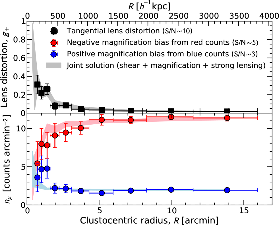
Figure 1.— Cluster weak-lensing radial profiles of MACS1206 ($z_{l}=0.439$) obtained from a reanalysis of the Subaru $BR_{\rm c}z^{\prime}$ data presented in Umetsu et al. (2012, see their Figures 4 and 5). The top panel shows the tangential reduced shear profile $g_{+}$ (squares) based on the full background sample. The bottom panel shows the coverage-corrected number-count profiles $n_{\mu}$ for flux-limited samples of blue and red background galaxies (circles). The error bars include contributions from Poisson counting uncertainties and contamination due to intrinsic angular clustering of each source population. For the red sample, a strong radial depletion of the source counts is seen toward the cluster center due primarily to magnification of the sky area, while a slight enhancement of blue counts is present in the innermost radial bins due to the effect of positive magnification bias. Also shown for each observed profile is the joint Bayesian reconstruction from combined strong-lensing, weak-lensing tangential distortion, positive and negative magnification-bias measurements (see also Figure 2).

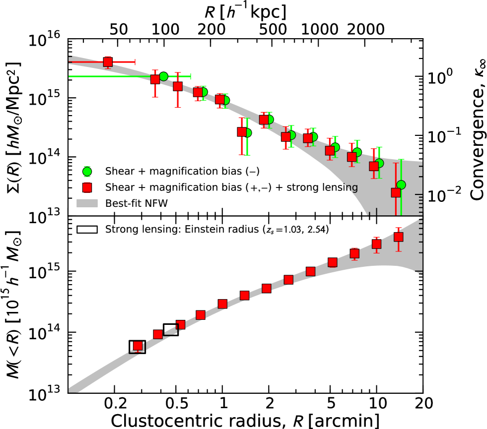
Figure 2.— Effects of including additional strong-lensing and positive magnification-bias constraints. The top panel shows the projected mass density profile $\Sigma(R)$ of MACS1206 derived from multi-probe cluster lensing measurements. For each case, the innermost central bin $\overline{\Sigma}(<R_{\rm min})$ is marked with a horizontal bar. The green circles show the $\Sigma(R)$ profile reconstructed from a joint likelihood analysis of weak-lensing distortion and negative magnification-bias measurements (Figure 1). The red squares are obtained from a joint analysis of the full lensing constraints, including additional strong-lensing (boxes, bottom) and positive magnification-bias (Figure 1) measurements. The central weak-lensing bin $\overline{\Sigma}(<0.6\arcmin)$ is resolved into 3 radial bins when additional double Einstein-radius constraints from strong lensing are included. For visual clarity, the reconstructed mass profiles are horizontally shifted by $4\%$ with respect to each other. The red area in the bottom panel shows the corresponding enclosed mass profile $M(<R)$. The boxes represent the double Einstein-radius constraints on the enclosed mass, corresponding to background sources at $z_{s}=1.03$ and $2.54$ (Umetsu et al., 2012, see their Figure 7). In each panel, the gray area represents the best-fit NFW (+ mass-sheet) profile derived from a joint analysis of the full-lensing constraints (red squares).

Appendix A Nonlinear Effect on the Source-averaged Lensing Fields

A.1. Reduced Shear

The reduced gravitational shear, $g=\gamma/(1-\kappa)$, is nonlinear in $\kappa$, so that the averaging operator with respect to the source redshift acts nonlinearly on $\kappa$. In general, a wide spread of the redshift distribution of background galaxies, in conjunction with the single source-plan approximation, may lead to an overestimation of the gravitational shear in the nonlinear regime (Hoekstra et al., 2000).

Too see this effect, we expand the reduced shear $g=g(z)$ with respect to $\kappa=\kappa(z)$ as

$$g=\gamma/(1-\kappa)=w\gamma_{\infty}(1-w\kappa_{\infty})^{-1}=w\gamma_{\infty}\sum_{k=0}^{\infty}\left(w\kappa_{\infty}\right)^{k}.$$ (A1)

Hence, the reduced shear averaged over the source redshift distribution is expressed as

$$\langle g\rangle=\gamma_{\infty}\sum_{k=0}^{\infty}\langle w^{k+1}\rangle\kappa_{\infty}^{k},$$ (A2)

where the angular brackets denote an ensemble average over the redshift distribution $N(z)$ of background sources. In the weak-lensing limit where $\kappa_{\infty},|\gamma_{\infty}|\ll 1$, $\langle g\rangle\approx\langle w\rangle\gamma_{\infty}=\langle\gamma\rangle$. The next order of approximation is given by

$$\langle g\rangle\approx\gamma_{\infty}\left(\langle w\rangle+\langle w^{2}\rangle\kappa_{\infty}^{2}\right)\approx\frac{\langle w\rangle\gamma_{\infty}}{1-\kappa_{\infty}\langle w^{2}\rangle/\langle w\rangle}.$$ (A3)

Seitz & Schneider (1997) found that Equation (A3) yields an excellent approximation in the mildly-nonlinear regime of $\kappa_{\infty}\lower 2.15277pt\hbox{$\;\buildrel<\over{\sim}\;$}0.6$. Defining $f_{w}\equiv\langle w^{2}\rangle/\langle w\rangle^{2}$, a dimensionless quantity of the order of unity, we have the following expression for the source-averaged reduced shear valid in the mildly-nonlinear regime:

$$\langle g\rangle\approx\frac{\langle\gamma\rangle}{1-f_{w}\langle\kappa\rangle},$$ (A4)

with $\langle\kappa\rangle=\langle w\rangle\kappa_{\infty}$ and $\langle\gamma\rangle=\langle w\rangle\gamma_{\infty}$ (Seitz & Schneider, 1997). For clusters lying at relatively low redshifts, $\langle w^{2}\rangle\approx\langle w\rangle^{2}$ and $f_{w}\approx 1$, leading to the single source-plane approximation: $\langle g\rangle\approx\langle\gamma\rangle/(1-\langle\kappa\rangle)$. The level of bias introduced by this approximation is $\Delta g/g\approx(f_{w}-1)\langle\kappa\rangle$. In typical ground-based deep observations of $z_{l}\lower 2.15277pt\hbox{$\;\buildrel<\over{\sim}\;$}0.5$ clusters (Okabe et al., 2010; Medezinski et al., 2010; Umetsu et al., 2010, 2011a, 2012), $\Delta f_{w}\equiv f_{w}-1$ is found to be of the order of several percent, so that the relative error in the $g$ estimate is negligibly small in the mildly-nonlinear regime.

A.2. Magnification Bias

First, let us consider a maximally-depleted sample of background sources with $s=d\log_{10}N(<m)/dm=0$, for which the effect of magnification bias is purely geometric, $b_{\mu}=\mu^{-1}$, and is insensitive to the intrinsic source luminosity function. In the nonlinear subcritical regime, the source-averaged magnification bias is expressed as

$$\langle b_{\mu}\rangle=\langle\mu^{-1}\rangle=1-2\langle\kappa\rangle-f_{w}\left(|\langle\gamma\rangle|^{2}-\langle\kappa\rangle^{2}\right)=\mu^{-1}(\langle w\rangle)+(f_{w}-1)\left(\langle\kappa\rangle^{2}-|\langle\gamma\rangle|^{2}\right),$$ (A5)

where $\mu^{-1}(\langle w\rangle)=(1-\langle\kappa\rangle)^{2}-|\langle\gamma\rangle|^{2}$. The error associated with the single source-plane approximation is therefore $\Delta b_{\mu}=(f_{w}-1)(\langle\kappa\rangle^{2}-|\langle\gamma\rangle|^{2})=\Delta f_{w}(\langle\kappa\rangle^{2}-|\langle\gamma\rangle|^{2})$, which is much smaller than unity for background source populations of our concern in the mildly-nonlinear subcritical regime ($\langle\kappa\rangle\sim|\langle\gamma\rangle|\sim O(10^{-1})$). It is therefore reasonable to use the single source-plane approximation for calculating the magnification bias of depleted source populations with $s\ll 0.4$.

In the positive regime of magnification bias ($s>0.4$), on the other hand, interpreting the observed lensing signal (i.e., the density enhancement) is more difficult, especially in the nonlinear regime where the flux amplification factor is correspondingly large (say, $\mu\lower 2.15277pt\hbox{$\;\buildrel>\over{\sim}\;$}1.5$). Therefore, it requires detailed information about the intrinsic source luminosity function to apply nonlinear corrections due to the spread of the source redshift distribution. In practice, the distant blue population of background galaxies has a distinct, well-defined redshift distribution, which is fairly symmetric and peaked at a mean redshift of $\langle z_{s}\rangle\sim 2$ (Lilly et al., 2007; Medezinski et al., 2010; Umetsu et al., 2010), so that the majority of faint blue galaxies are in the far background of typical cluster lenses, and that the lensing signal has a weaker dependence on the source redshift. In such a case, the single source-plane approximation may be justified.

Appendix B Discretized Expressions for the Cluster Lensing Profiles

B.1. Averaged Convergence

In this appendix, we aim to derive a discrete expression for the mean interior convergence $\overline{\kappa}_{\infty}(<\theta)$ as a function of clustocentric radius $\theta$ using the azimuthally-averaged convergence $\kappa_{\infty}(\theta)$. In the continuous limit, the mean convergence $\bar{\kappa}_{\infty}(<\theta)$ interior to radius $\theta$ can be expressed in terms of $\kappa_{\infty}(\theta)$ as

$$\overline{\kappa}_{\infty}(\theta)=\frac{2}{\theta^{2}}\int_{0}^{\theta}\!d\ln\theta^{\prime}\theta^{\prime 2}\kappa_{\infty}(\theta^{\prime}).$$ (B1)

For a given set of $(N+1)$ annular radii $\theta_{l}$ $(l=1,2,...,N+1)$, defining $N$ radial bands in the range $\theta_{\rm min}\equiv\theta_{1}\leq\theta\leq\theta_{N+1}\equiv\theta_{\rm max}$, a discretized estimator for $\overline{\kappa}_{\infty}(<\theta)$ can be written in the following way:

$$\overline{\kappa}_{\infty}(<\theta_{l})=\frac{\theta_{\rm min}^{2}}{\theta_{l}^{2}}\overline{\kappa}_{\infty}(<\theta_{\rm min})+\frac{2}{\theta_{l}^{2}}\sum_{i=1}^{l-1}\Delta\ln\theta_{i}\bar{\theta}_{i}^{2}\kappa_{\infty}(\bar{\theta}_{i}),$$ (B2)

with $\Delta\ln\theta_{i}\equiv(\theta_{i+1}-\theta_{i})/\bar{\theta}_{i}$ and $\bar{\theta}_{i}$ being the area-weighted center of the $i$th annulus defined by $\theta_{i}$ and $\theta_{i+1}$; in the continuous limit, we have

$$\bar{\theta}_{i}\equiv 2\int_{\theta_{i}}^{\theta_{i+1}}\!d\theta^{\prime}\theta^{\prime 2}/(\theta_{i+1}^{2}-\theta_{i}^{2})\\ =\frac{2}{3}\frac{\theta_{i}^{2}+\theta_{i+1}^{2}+\theta_{i}\theta_{i+1}}{\theta_{i}+\theta_{i+1}}.$$

B.2. Lens Distortion and Magnification

We derive expressions for the binned tangential distortion $g_{+}(\theta;w_{g})$ and magnification $\mu(\theta;w_{\mu})$ in terms of the binned convergence $\kappa_{\infty}$, using the following relations:

$$g_{+}(\overline{\theta}_{i};w_{g}) = \frac{w_{g}\left[\overline{\kappa}_{\infty}(<\overline{\theta}_{i})-\kappa_{\infty}(\overline{\theta}_{i})\right]}{1-w_{g}\kappa_{\infty}(\overline{\theta}_{i})},$$ (B3)

$$\mu(\overline{\theta}_{i};w_{\mu}) = \frac{1}{\left[1-w_{\mu}\kappa_{\infty}(\overline{\theta}_{i})\right]^{2}\left[1-g_{+}^{2}(\overline{\theta}_{i};w_{\mu})\right]},$$ (B4)

where both the quantities depend on the mean convergence $\overline{\kappa}_{\infty}$ interior to the radius $\overline{\theta}_{i}$, which is the center of the $i$th radial band of $[\theta_{i},\theta_{i+1}]$ (see Appendix B.1). By assuming a constant density in each radial band and by noting that $\overline{\theta}_{i}$ is the median radius of the $i$th radial band, $\overline{\kappa}(<\overline{\theta}_{i})$ can be well approximated by (Umetsu et al., 2011a)

$$\overline{\kappa}_{\infty}(<\overline{\theta}_{i})=\frac{1}{2}\Big{[}\overline{\kappa}_{\infty}(<\theta_{i})+\overline{\kappa}_{\infty}(<\theta_{i+1})\Big{]},$$ (B5)

where $\overline{\kappa}_{\infty}(<\theta_{i})$ and $\overline{\kappa}_{\infty}(<\theta_{i+1})$ can be computed using the formulae given in this appendix.

Accordingly, all relevant cluster lensing observables, $g_{+}(\theta),n_{\mu}(\theta)$, and $M(<\theta)$, can be uniquely specified by the discrete convergence profile, $\mbox{\boldmath$s$}=\{\overline{\kappa}_{\infty,{\rm min}},\kappa_{\infty,i}\}_{i=1}^{N}$ with $\overline{\kappa}_{\infty,{\rm min}}\equiv\overline{\kappa}_{\infty}(\theta_{\rm min})$ and $\kappa_{\infty,i}\equiv\kappa_{\infty}(\theta_{i})$.

References

- Allen et al. (2008) Allen, S. W., Rapetti, D. A., Schmidt, R. W., et al. 2008, MNRAS, 383, 879
- Bartelmann et al. (2001) Bartelmann, M., King, L. J., & Schneider, P. 2001, A&A, 378, 361
- Bartelmann & Schneider (2001) Bartelmann, M., & Schneider, P. 2001, Phys. Rep., 340, 291
- Broadhurst (1995) Broadhurst, T. 1995, ArXiv Astrophysics e-prints, arXiv:astro-ph/9511150
- Broadhurst et al. (2005a) Broadhurst, T., Takada, M., Umetsu, K., et al. 2005a, ApJ, 619, L143
- Broadhurst et al. (2005b) Broadhurst, T., Benítez, N., Coe, D., et al. 2005b, ApJ, 621, 53
- Broadhurst & Barkana (2008) Broadhurst, T. J., & Barkana, R. 2008, MNRAS, 390, 1647
- Broadhurst et al. (1995) Broadhurst, T. J., Taylor, A. N., & Peacock, J. A. 1995, ApJ, 438, 49
- Clowe et al. (2006) Clowe, D., Bradač, M., Gonzalez, A. H., et al. 2006, ApJ, 648, L109
- Coe et al. (2010) Coe, D., Benítez, N., Broadhurst, T., & Moustakas, L. A. 2010, ApJ, 723, 1678
- Coe et al. (2012) Coe, D., Umetsu, K., Zitrin, A., et al. 2012, ApJ, 757, 22
- Ebeling et al. (2009) Ebeling, H., Ma, C. J., Kneib, J.-P., et al. 2009, MNRAS, 395, 1213
- Faltenbacher et al. (2009) Faltenbacher, A., Li, C., White, S. D. M., et al. 2009, Research in Astronomy and Astrophysics, 9, 41
- Ford et al. (2012) Ford, J., Hildebrandt, H., Van Waerbeke, L., et al. 2012, ApJ, 754, 143
- Gao et al. (2012) Gao, L., Navarro, J. F., Frenk, C. S., et al. 2012, MNRAS, 425, 2169
- Gavazzi et al. (2003) Gavazzi, R., Fort, B., Mellier, Y., Pelló, R., & Dantel-Fort, M. 2003, A&A, 403, 11
- Geller et al. (2013) Geller, M. J., Diaferio, A., Rines, K. J., & Serra, A. L. 2013, ApJ, 764, 58
- Gilmour et al. (2009) Gilmour, R., Best, P., & Almaini, O. 2009, MNRAS, 392, 1509
- Graham et al. (2006) Graham, A. W., Merritt, D., Moore, B., Diemand, J., & Terzić, B. 2006, AJ, 132, 2701
- Hildebrandt et al. (2009) Hildebrandt, H., van Waerbeke, L., & Erben, T. 2009, A&A, 507, 683
- Hildebrandt et al. (2011) Hildebrandt, H., Muzzin, A., Erben, T., et al. 2011, ApJ, 733, L30
- Hoekstra et al. (2000) Hoekstra, H., Franx, M., & Kuijken, K. 2000, ApJ, 532, 88
- Hu et al. (2000) Hu, W., Barkana, R., & Gruzinov, A. 2000, Physical Review Letters, 85, 1158
- Huff & Graves (2011) Huff, E. M., & Graves, G. J. 2011, ArXiv e-prints, arXiv:1111.1070 [astro-ph.CO]
- Ilbert et al. (2009) Ilbert, O., Capak, P., Salvato, M., et al. 2009, ApJ, 690, 1236
- Jing & Suto (2000) Jing, Y. P., & Suto, Y. 2000, ApJ, 529, L69
- Jullo et al. (2007) Jullo, E., Kneib, J.-P., Limousin, M., et al. 2007, New Journal of Physics, 9, 447
- Kaiser (1995) Kaiser, N. 1995, ApJ, 439, L1
- Kaiser et al. (1995) Kaiser, N., Squires, G., & Broadhurst, T. 1995, ApJ, 449, 460
- Klypin et al. (1999) Klypin, A., Kravtsov, A. V., Valenzuela, O., & Prada, F. 1999, ApJ, 522, 82
- Kneib & Natarajan (2011) Kneib, J.-P., & Natarajan, P. 2011, A&A Rev., 19, 47
- Lapi & Cavaliere (2009) Lapi, A., & Cavaliere, A. 2009, ApJ, 692, 174
- Lemze et al. (2008) Lemze, D., Barkana, R., Broadhurst, T. J., & Rephaeli, Y. 2008, MNRAS, 386, 1092
- Liesenborgs & De Rijcke (2012) Liesenborgs, J., & De Rijcke, S. 2012, MNRAS, 425, 1772
- Lilly et al. (2007) Lilly, S. J., Le Fèvre, O., Renzini, A., et al. 2007, ApJS, 172, 70
- Limousin et al. (2007) Limousin, M., Richard, J., Jullo, E., et al. 2007, ApJ, 668, 643
- Medezinski et al. (2011) Medezinski, E., Broadhurst, T., Umetsu, K., Benítez, N., & Taylor, A. 2011, MNRAS, 414, 1840
- Medezinski et al. (2010) Medezinski, E., Broadhurst, T., Umetsu, K., et al. 2010, MNRAS, 405, 257
- Medezinski et al. (2013) Medezinski, E., Umetsu, K., Nonino, M., et al. 2013, ArXiv e-prints, arXiv:1304.1223 [astro-ph.CO]
- Ménard & Bartelmann (2002) Ménard, B., & Bartelmann, M. 2002, A&A, 386, 784
- Merten et al. (2009) Merten, J., Cacciato, M., Meneghetti, M., Mignone, C., & Bartelmann, M. 2009, A&A, 500, 681
- Miyazaki et al. (2002) Miyazaki, S., Komiyama, Y., Sekiguchi, M., et al. 2002, PASJ, 54, 833
- Morrison et al. (2012) Morrison, C. B., Scranton, R., Ménard, B., et al. 2012, MNRAS, 426, 2489
- Narayan & Bartelmann (1996) Narayan, R., & Bartelmann, M. 1996, ArXiv Astrophysics e-prints, arXiv:astro-ph/9606001
- Narikawa & Yamamoto (2012) Narikawa, T., & Yamamoto, K. 2012, J. Cosmology Astropart. Phys, 5, 16
- Navarro et al. (1997) Navarro, J. F., Frenk, C. S., & White, S. D. M. 1997, ApJ, 490, 493
- Navarro et al. (2010) Navarro, J. F., Ludlow, A., Springel, V., et al. 2010, MNRAS, 402, 21
- Newman et al. (2012a) Newman, A. B., Treu, T., Ellis, R. S., & Sand, D. J. 2012a, ArXiv e-prints, arXiv:1209.1392 [astro-ph.CO]
- Newman et al. (2012b) Newman, A. B., Treu, T., Ellis, R. S., et al. 2012b, ArXiv e-prints, arXiv:1209.1391 [astro-ph.CO]
- Newman et al. (2009) —. 2009, ApJ, 706, 1078
- Oguri (2010) Oguri, M. 2010, PASJ, 62, 1017
- Oguri et al. (2012) Oguri, M., Bayliss, M. B., Dahle, H., et al. 2012, MNRAS, 420, 3213
- Oguri & Blandford (2009) Oguri, M., & Blandford, R. D. 2009, MNRAS, 392, 930
- Oguri & Hamana (2011) Oguri, M., & Hamana, T. 2011, MNRAS, 414, 1851
- Oguri & Takada (2011) Oguri, M., & Takada, M. 2011, Phys. Rev. D, 83, 023008
- Oguri et al. (2009) Oguri, M., Hennawi, J. F., Gladders, M. D., et al. 2009, ApJ, 699, 1038
- Okabe et al. (2010) Okabe, N., Takada, M., Umetsu, K., Futamase, T., & Smith, G. P. 2010, PASJ, 62, 811
- Okabe & Umetsu (2008) Okabe, N., & Umetsu, K. 2008, PASJ, 60, 345
- Peebles & Nusser (2010) Peebles, P. J. E., & Nusser, A. 2010, Nature, 465, 565
- Postman et al. (2012) Postman, M., Coe, D., Benítez, N., et al. 2012, ApJS, 199, 25
- Rozo et al. (2012) Rozo, E., Bartlett, J. G., Evrard, A. E., & Rykoff, E. S. 2012, ArXiv e-prints, arXiv:1204.6305 [astro-ph.CO]
- Rozo & Schmidt (2010) Rozo, E., & Schmidt, F. 2010, arXiv, 1009.5735, arXiv:1009.5735 [astro-ph.CO]
- Saha & Read (2009) Saha, P., & Read, J. I. 2009, ApJ, 690, 154
- Saha & Williams (2006) Saha, P., & Williams, L. L. R. 2006, ApJ, 653, 936
- Schmidt et al. (2012) Schmidt, F., Leauthaud, A., Massey, R., et al. 2012, ApJ, 744, L22
- Schneider et al. (2000) Schneider, P., King, L., & Erben, T. 2000, A&A, 353, 41
- Schneider & Seitz (1995) Schneider, P., & Seitz, C. 1995, A&A, 294, 411
- Scranton et al. (2005) Scranton, R., Ménard, B., Richards, G. T., et al. 2005, ApJ, 633, 589
- Seitz & Schneider (1997) Seitz, C., & Schneider, P. 1997, A&A, 318, 687
- Sereno & Umetsu (2011) Sereno, M., & Umetsu, K. 2011, MNRAS, 416, 3187
- Silva et al. (2013) Silva, L. J. B. e., Lima, M., & Sodré, L. 2013, ArXiv e-prints, arXiv:1301.1684 [astro-ph.CO]
- Tasitsiomi et al. (2004) Tasitsiomi, A., Kravtsov, A. V., Gottlöber, S., & Klypin, A. A. 2004, ApJ, 607, 125
- Tinker et al. (2010) Tinker, J. L., Robertson, B. E., Kravtsov, A. V., et al. 2010, ApJ, 724, 878
- Umetsu (2010) Umetsu, K. 2010, ArXiv e-prints, arXiv:1002.3952 [astro-ph.CO]
- Umetsu & Broadhurst (2008) Umetsu, K., & Broadhurst, T. 2008, ApJ, 684, 177
- Umetsu et al. (2011a) Umetsu, K., Broadhurst, T., Zitrin, A., Medezinski, E., & Hsu, L. 2011a, ApJ, 729, 127
- Umetsu et al. (2011b) Umetsu, K., Broadhurst, T., Zitrin, A., et al. 2011b, ApJ, 738, 41
- Umetsu & Futamase (2000) Umetsu, K., & Futamase, T. 2000, ApJ, 539, L5
- Umetsu et al. (2010) Umetsu, K., Medezinski, E., Broadhurst, T., et al. 2010, ApJ, 714, 1470
- Umetsu et al. (2012) Umetsu, K., Medezinski, E., Nonino, M., et al. 2012, ApJ, 755, 56
- Van Waerbeke et al. (2010) Van Waerbeke, L., Hildebrandt, H., Ford, J., & Milkeraitis, M. 2010, ApJ, 723, L13
- Vikhlinin et al. (2009) Vikhlinin, A., Kravtsov, A. V., Burenin, R. A., et al. 2009, ApJ, 692, 1060
- von der Linden et al. (2012) von der Linden, A., Allen, M. T., Applegate, D. E., et al. 2012, ArXiv e-prints, arXiv:1208.0597 [astro-ph.CO]
- Woo & Chiueh (2009) Woo, T., & Chiueh, T. 2009, ApJ, 697, 850
- Zitrin et al. (2011a) Zitrin, A., Broadhurst, T., Barkana, R., Rephaeli, Y., & Benítez, N. 2011a, MNRAS, 410, 1939
- Zitrin et al. (2009) Zitrin, A., Broadhurst, T., Umetsu, K., et al. 2009, MNRAS, 396, 1985
- Zitrin et al. (2010) —. 2010, MNRAS, 408, 1916
- Zitrin et al. (2011b) Zitrin, A., Broadhurst, T., Coe, D., et al. 2011b, ApJ, 742, 117
- Zitrin et al. (2012) Zitrin, A., Rosati, P., Nonino, M., et al. 2012, ApJ, 749, 97
- Zitrin et al. (2013) Zitrin, A., Meneghetti, M., Umetsu, K., et al. 2013, ApJ, 762, L30