Semiclassical quantization and spectral limits of $\hbar$-pseudodifferential and Berezin-Toeplitz operators

Abstract.

We introduce a minimalistic notion of semiclassical quantization and use it to prove that the convex hull of the semiclassical spectrum of a quantum system given by a collection of commuting operators converges to the convex hull of the spectrum of the associated classical system. This gives a quick alternative solution to the isospectrality problem for quantum toric systems. If the operators are uniformly bounded, the convergence is uniform. Analogous results hold for non-commuting operators.

1. Introduction

In the past ten years there has been a flurry of activity concerning the interaction between symplectic geometry and spectral theory. The potential of this interaction was already pointed out by Colin de Verdière [14, 13] in a quite general setting: pseudodifferetial operators on cotangent bundles. This paper deals with the question: can one recover a classical system (described by symplectic geometry) from the spectrum of its quantization (described by spectral theory)? This is a classical question in inverse spectral theory going back to pioneer works of Colin de Verdière and Guillemin-Sternberg, in the 1970s and 1980s.

Many contributions followed their works, eg Iantchenko–Sjöstrand–Zworski [24]. A few global spectral results have also been obtained recently, for instance by Hezari and Zelditch for symmetric domains in ${\mathbb{R}}^{n}$ [21] or by Vũ Ngọc [36] for one degree of freedom pseudodifferential operators. Recently, the first and third author settled, jointly with L. Charles, this problem for toric integrable systems [12]. The paper [12] gives a full description of the semiclassical spectral theory of toric integrable systems. As a corollary of this theory, that paper solves the isospectral theorem for toric systems. We refer to Section 8.2 for more details, and to [12] for a more complete list of references on inverse spectral results in symplectic geometry. For an interesting semiclassical recent work see the article of Guillemin, Paul, and Uribe [19] on trace invariants.

The goal of the present paper is to introduce a minimalistic notion of semiclassical quantization and use it to provide a simple constructive argument proving that from the joint spectrum of a quantum system one can recover the convex hull of the classical spectrum. This applies not only to toric integrable systems, but much more generally. Moreover, our results are general enough to apply to pseudodifferential and Berezin-Toeplitz quantization.

Structure of the paper.

In section 2 we quickly state our main results in the most important particular cases: pseudodifferential and Berezin-Toeplitz quantization: Theorem 1 and Theorem 2. In Section 3 we recall some preliminaries on self-adjoint operators. In Section 4 we introduce a general quantization setting and state results that encompass Theorem 1 and Theorem 2. In Section 5 we prove a key lemma concerning spectral limits of semiclassical operators. Section 6 reviews properties of support functions and convex sets which are needed for the proofs. In Section 7 we combine the previous sections to complete the proofs. In Sections 8 and 9 we briefly review the Berezin-Toeplitz quantization and $\hbar$-pseudo-differential calculus and show that they are covered by the quantization procedure of Section 4.

We present a number of examples illustrating our results: Section 8.2 explains how to use Theorem 1 to conclude, quickly, the isospectrality theorem for toric systems which appeared in a previous work [12] of the first and third author and L. Charles. In Section 8.3 we apply our results to a physically interesting system, coupled angular momenta on $S^{2}\times S^{2}$ described by D.A. Sadovskií and B.I. Zhilinskií in [30]. Section 9.2 deals with $\hbar$-pseudodifferential quantization of a particle on the plane in a rotationally symmetric potential.

In the last section we extend our results to nonnecessarily commuting operators.

2. Main results

For simplicity, in this section we will only state our results in the two (otherwise rather general) cases of pseudodifferential and Berezin-Toeplitz quantization. In the statements below, we fix a quantization scheme for a symplectic manifold $M$ and focus on a collection $\mathcal{F}=(T_{1},\dots,T_{d})$ of mutually commuting self-adjoint semi-classical operators. These operators depend on the Planck constant $\hbar\in I$, where $I$ is a subset of $(0,1]$ that accumulates at $0$, and act on a Hilbert space $\mathcal{H}_{\hbar},\;\hbar\in I$.

Let $T_{1},\ldots,T_{d}$ are pair-wise commuting selfadjoint (not necessarily bounded) operators on a Hilbert space $\mathcal{H}$ with a common dense domain $\mathcal{D}\subset\mathcal{H}$ such that $T_{j}(\mathcal{D})\subset\mathcal{D}$ for all $j$. The joint spectrum of $(T_{1},\ldots,T_{d})$ is by definition the support of the joint spectral measure. It is denoted by $\!\!\mathop{\rm~{}JointSpec}\nolimits(T_{1},\,\ldots,\,T_{d})$.

For instance, if $T_{j}$’s are endomorphisms of a finite dimensional vector space, then the joint spectrum of $T_{1},\ldots,T_{d}$ is the set of $(\lambda_{1},\dots,\lambda_{d})\in\mathbb{C}^{d}$ such that there exists a non-zero vector $v$ for which

$$T_{j}v=\lambda_{j}v,\quad\forall j=1,\dots,n.$$

If $T_{1},\,\ldots,\,T_{d}$ are pairwise commuting semiclassical operators, then of course the joint spectrum of $T_{1},\ldots,T_{d}$ depends on $\hbar$.

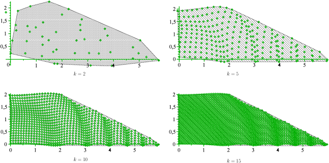
Figure 1. Convergence of convex hulls of semiclassical spectra ($k=1/\hbar$) of a quantum toric system [12].

Following the physicists, we shall call classical spectrum of $(T_{1},\dots,T_{d})$ the image $F(M)\subset{\mathbb{R}}^{d}$, where $F=(f^{(1)},\dots,f^{(d)})$ is the map of principal symbols of $T_{1},\dots,T_{d}$.

Theorem 1.

Let $M$ be a prequantizable closed symplectic manifold. Let $d\geqslant 1$ and let $\mathcal{F}:=(T_{1},\dots,T_{d})$ be a family of pairwise commuting selfadjoint Berezin-Toeplitz operators on $M$. Let $\mathcal{S}\subset{\mathbb{R}}^{d}$ be the classical spectrum of $\mathcal{F}$. Then

(1) $$\lim_{\hbar\rightarrow 0}{\rm Convex\,\,Hull}\,\Big{(}\textup{JointSpec}(\mathcal{F})\Big{)}\,=\,{\rm Convex\,\,Hull}\,\left(\mathcal{S}\right)$$

where the limit convergence is in the Hausdorff metric.

In the $\hbar$-pseudodifferential setting (see for instance [17]), the analysis is more complicated due to the possible unboundedness of the operators. Here we work with the standard Hörmander class of symbols $a(x,\xi,\hbar)$ on $\mathbb{R}^{2n}$ or ${\rm T}^{*}X$ with closed $X$ imposing the following restriction on the dependence of $a$ on $\hbar$:

$$a(x,\xi,\hbar)=a_{0}(x,\xi)+\hbar a_{1,\hbar}(x,\xi)\;,$$

where all $a_{1,\hbar}(x,\xi)$ are uniformly (in $\hbar$) bounded and supported in the same compact set. The principal symbol $a_{0}$ can be unbounded. We shall say that $a$ mildly depends on $\hbar$. Fortunately, in a number of meaningful examples one deals with $\hbar$-independent symbols, see e.g. Section 9.2 below.

Theorem 2.

Let $X$ be either $\mathbb{R}^{n}$, $n\geqslant 1$, or a closed manifold. Let $d\geqslant 1$ and let $\mathcal{F}:=(T_{1},\dots T_{d})$ be a family of pairwise commuting selfadjoint $\hbar$-pseudodifferential operators on $X$ whose symbols mildly depend on $\hbar$. Then the following hold.

• From the family

  $$\Big{\{}{\rm Convex\,\,Hull}\,\Big{(}\textup{JointSpec}(\mathcal{F})\Big{)}\Big{\}}_{\hbar\in J}$$

  one can recover the convex hull of the classical spectrum of $\mathcal{F}$.

• If, in addition, the principal symbols of $T_{j}$ are bounded for every $1\leqslant j\leqslant d$, the joint and the classical spectra are related by equation (1).

The assumption on mild dependence of the symbol on $\hbar$ cannot be completely dropped, see Remark 9.1 below. An immediate consequence of the theorems is the following simple statement.

Corollary 3.

Let $T_{1},\dots,T_{d}$ be either:

• commuting self-adjoint Berezin-Toeplitz operators on a prequantizable closed symplectic manifold, or

• $\hbar$-pseudodifferential self-adjoint operators on $\mathbb{R}^{n}$ or a closed manifold whose symbols mildly depend on $\hbar$.

If the classical spectrum of $(T_{1},\dots,T_{d})$ is convex, then the joint spectrum recovers it.

3. Preliminaries on self-adjoint operators

First let us recall some elementary results from operator theory. For any (not necessarily bounded) selfadjoint operator $A$ on a Hilbert space with a dense domain and with spectrum $\sigma(A)$, we have

(2) $$\sup\sigma(A)=\sup_{u\neq 0}\frac{\langle Au,u\rangle}{\langle u,u\rangle}\;.$$

This follows for instance from [22, Proposition 5.12]. We give the proof here for the reader’s convenience. If $\lambda\in\sigma(A)$, then by the Weyl criterium, there exists a sequence $(u_{n})$ with $\|u_{n}\|=1$ such that

$$\lim_{n\to\infty}\|(A-\lambda{\rm Id})u_{n}\|=0.$$

Therefore, $\lim_{n\to\infty}\langle Au_{n},u_{n}\rangle=\lambda$, which implies that

$$\sup_{\|u\|=1}\langle Au,u\rangle\geqslant\sup\sigma(A).$$

Conversely, if $\sigma(A)$ lies in $(-\infty,c]$, then by the Spectral Theorem $A\leqslant c\cdot{{\rm Id}}$ which yields

$$\sup_{\|u\|=1}\langle Au,u\rangle\leqslant\sup\sigma(A).$$

This proves (2).

Let us mention also that it implies

(3) $$\sup\{|s|:s\in\sigma(A)\}=\sup_{u\neq 0}\frac{|\langle Au,u\rangle|}{\langle u,u\rangle}=\|A\|\leqslant\infty;.$$

4. Semiclassical quantization

We shall prove Theorem 1 and Theorem 2 in a more general context of semiclassical quantization.

Let $M$ be a connected manifold (either closed or open). Let $\mathcal{A}_{0}$ be a subalgebra of $\textup{C}^{\infty}(M;{\mathbb{R}})$ containing the constants and all compactly supported functions. We fix a subset $I\subset(0,1]$ that accumulates at $0$. If $\mathcal{H}$ is a complex Hilbert space, we denote by $\mathcal{L}(\mathcal{H})$ the set of linear (possibly unbounded) selfadjoint operators on $\mathcal{H}$ with a dense domain. By a slight abuse of notation, we write $\|T\|$ for the operator norm of an operator, and $\|f\|$ for the uniform norm of a function on $M$.

Definition 4. A semiclassical quantization of $(M,\mathcal{A}_{0})$ consists of a family of complex Hilbert spaces $\mathcal{H}_{\hbar},\;\hbar\in I$, and a family of ${\mathbb{R}}$-linear maps ${\rm Op}_{\hbar}\colon\mathcal{A}_{0}\to\mathcal{L}(\mathcal{H}_{\hbar})$ satisfying the following properties, where $f$ and $g$ are in $\mathcal{A}_{0}$:

1. $\|{\rm Op}_{\hbar}(1)-{\rm Id}\|=\mathcal{O}(\hbar)$ (normalization);

2. for all $f\geqslant 0$ there exists a constant $C_{f}$ such that ${\rm Op}_{\hbar}(f)\geqslant-C_{f}\hbar$ (quasi-positivity);

3. let $f\in\mathcal{A}_{0}$ such that $f\neq 0$ and has compact support, then

   $$\liminf_{\hbar\to 0}\|{\rm Op}_{\hbar}(f)\|>0$$

   (non-degeneracy);

4. if $g$ has compact support, then for all $f$, ${\rm Op}_{\hbar}(f)\circ{\rm Op}_{\hbar}(g)$ is bounded, and we have

   $$\|{\rm Op}_{\hbar}(f)\circ{\rm Op}_{\hbar}(g)-{\rm Op}_{\hbar}(fg)\|=\mathcal{O}(\hbar),$$

   (product formula).

A quantizable manifold is a manifold for which there exists a semiclassical quantization.

We shall often use the following consequence of these axioms: for a bounded function $f$, the operator ${\rm Op}_{\hbar}(f)$ is bounded. Indeed, if $c_{1}\leqslant f\leqslant c_{2}$ for some $c_{1},c_{2}\in\mathbb{R}$, (Q1) and (Q2) yield

(4) $$c_{1}\cdot{{\rm Id}}-\mathcal{O}(\hbar)\leqslant{\rm Op}_{\hbar}(f)\leqslant c_{2}\cdot{{\rm Id}}+\mathcal{O}(\hbar).$$

Since our operators are selfadjoint, this implies by formula (3) above

(5) $$\|{\rm Op}_{\hbar}(f)\|\leqslant\|f\|+{\mathcal{O}}(\hbar)\;.$$

Next, consider the algebra $\mathcal{A}_{I}$ whose elements are collections $\vec{f}=(f_{\hbar})_{\hbar\in I}$, $f_{\hbar}\in\mathcal{A}_{0}$ with the following property: for each ${\vec{f}}$ there exists $f_{0}\in\mathcal{A}_{0}$ so that

(6) $$f_{\hbar}=f_{0}+\hbar f_{1,\hbar}\;,$$

where the sequence $f_{1,\hbar}$ is uniformly bounded in $\hbar$ and supported in the same compact set $K=K({\vec{f}})\subset M$. The function $f_{0}$ is called the principal part of ${\vec{f}}$. If $f_{0}$ is compactly supported as well, we say that ${\vec{f}}$ is compactly supported.

Definition 5. We define a map

$$\text{Op}:\mathcal{A}_{I}\to\prod_{\hbar\in I}\mathcal{L}(\mathcal{H}_{\hbar}),\;\;{\vec{f}}=(f_{\hbar})\mapsto({\rm Op}_{\hbar}(f_{\hbar}))\;.$$

A semiclassical operator is an element in the image of Op. Given ${\vec{f}}\in{\mathcal{A}}_{I}$, the function $f_{0}\in{\mathcal{A}}_{0}$ defined by (6) is called the principal symbol of $\text{Op}({\vec{f}})$.

By (5)

(7) $${\rm Op}_{\hbar}(f_{\hbar})={\rm Op}_{\hbar}(f_{0})+{\mathcal{O}}(\hbar)\;.$$

This together with the product formula (Q4) readily yields that for every $\vec{g}$ with compact support and every ${\vec{f}}$,

(8) $$\|{\rm Op}_{\hbar}(f_{\hbar})\circ{\rm Op}_{\hbar}(g_{\hbar})-{\rm Op}_{\hbar}(f_{\hbar}g_{\hbar})\|=\mathcal{O}(\hbar)\;.$$

Now we are ready to show that the principal symbol of a semiclassical operator is unique. Indeed, if $\text{Op}({\vec{f}})=0$, then for any compactly supported function $\chi$, we get by (8)

$${\rm Op}_{\hbar}(f_{\hbar}\chi)={\rm Op}_{\hbar}(f_{\hbar}){\rm Op}_{\hbar}(\chi)+\mathcal{O}(\hbar)=\mathcal{O}(\hbar),$$

and then by (7), ${\rm Op}_{\hbar}(f_{0}\chi)=\mathcal{O}(\hbar)$. By (Q3) we conclude that $f_{0}\chi=0$. Since $\chi$ is arbitrary, $f_{0}=0$.

Important examples of semiclassical quantization in the sense of Definition 4 are provided by symplectic geometry. They include Berezin-Toeplitz quantization on closed prequantizable symplectic manifolds and (certain versions of) $\hbar$-pseudodifferential calculus on cotangent bundles. In the latter case the algebra ${\mathcal{A}}_{0}$ is the usual Hörmander class of symbols, while its deformation ${\mathcal{A}}_{I}$ is more special and is defined as above. The details will be explained in Sections 8 and 9.

Remark 6. The definition of semiclassical quantization above is “minimalistic”: we list only those axioms which will enable us to reconstruct the classical spectrum from the quantum one, which is the main objective of the paper. In particular, we do not require a stronger form of the correspondence principle which links together commutators of semiclassical operators with Poisson brackets of their symbols, and even do not assume that the manifold $M$ is symplectic. $\oslash$

For the following results recall the notion of quantizable manifold we use (Definition 4).

Theorem 7.

Let $M$ be a quantizable manifold. Let $d\geqslant 1$ and let $(T_{1},\dots T_{d})$ be pairwise commuting semiclassical operators on $M$. Let $J$ be a subset of $I$ that accumulates at $0$. Then from the family

$$\Big{\{}{\rm Convex\,\,Hull}\,\Big{(}\textup{JointSpec}(T_{1},\dots,T_{d})\Big{)}\Big{\}}_{\hbar\in J}$$

one can recover the convex hull of the classical spectrum of $(T_{1},\dots,T_{d})$.

We can strengthen Theorem 7 in case the principal symbols are bounded to obtain a uniform convergence in the Hausdorff distance.

Recall that the Hausdorff distance between two subsets $A$ and $B$ of ${\mathbb{R}}^{d}$ is

$${\rm d}_{H}(A,\,B):=\inf\{\epsilon>0\,\,|\,\ A\subseteq B_{\epsilon}\ \mbox{and}\ B\subseteq A_{\epsilon}\},$$

where for any subset $X$ of ${\mathbb{R}}^{d}$, the set $X_{\epsilon}$ is

$$X_{\epsilon}:=\bigcup_{x\in X}\{m\in{\mathbb{R}}^{d}\,\,|\,\,\|x-m\|\leqslant\epsilon\},$$

(see eg. [7]).

Theorem 8.

Let $M$ be a quantizable manifold. Let $d\geqslant 1$ and let $(T_{1},\dots T_{d})$ be pairwise commuting semiclassical operators on $M$. Let $J$ be a subset of $I$ that accumulates at $0$. Assume that the principal symbols of $T_{j}$, $j=1,\dots,d$, are bounded. Let $\mathcal{S}\subset{\mathbb{R}}^{d}$ be the classical spectrum of $(T_{1},\dots,T_{d})$. Then

$$\lim_{\hbar\rightarrow 0}{\rm Convex\,\,Hull}\,\Big{(}\textup{JointSpec}(T_{1},\dots,T_{d})\Big{)}\,=\,{\rm Convex\,\,Hull}\,\left(\mathcal{S}\right)$$

where the limit convergence is in the Hausdorff metric.

Theorem 7 and Theorem 8 together with results of Sections 8.1 and 9.1 below readily yield Theorems 1 and 2 of the introduction.

Remark 9. Let $T$ be a uniformly (in $\hbar$) bounded selfadjoint operator with principal symbol $f$. Applying Theorem 8 with $d=1$, we get that

$$\lim_{\hbar\rightarrow 0}[\lambda_{\min}(T),\lambda_{\max}(T)]\,=\,{\mathcal{S}}=f(M),$$

where $\lambda_{\min}(T)$ and $\lambda_{\max}(T)$ are the minimum and maximum of the spectrum of $T$, respectively. Since by (3) the operator norm of a bounded selfadjoint operator equals $\max(\left|\lambda_{\min}\right|,\left|\lambda_{\max}\right|)$, we get that the axioms of semiclassical quantization listed in Definition 4 above imply the following “automatic” refinement of non-degeneracy axiom (Q3):

(9) $$\lim_{\hbar\to 0}\|{\rm Op}_{\hbar}(f)\|=\|f\|$$

for every bounded function $f\in\mathcal{A}_{0}$. $\oslash$

Corollary 10.

If the classical spectrum is convex, then the joint spectrum recovers it.

Corollary 10 is an immediate consequence of Theorem 7. Note that we don’t need to know the precise structure of the joint spectrum of the quantum system in order to recover the classical spectrum – it suffices to know the convex hull of this joint spectrum, as a subset of $\mathbb{R}^{d}$.

5. Spectral limits

Fix a semiclassical quantization the sense of Definition 4 on a manifold $M$.

Lemma 11.

Take any ${\vec{f}}=(f_{\hbar})\in\mathcal{A}_{I}$ with principal part $f_{0}$, and let $({\rm Op}_{\hbar}(f_{\hbar}))$ be the corresponding semiclassical operator. Let $\lambda_{\sup}(\hbar)$ denote the supremum of the spectrum of ${\rm Op}_{\hbar}(f_{\hbar})$. Then

(10) $$\lim_{\hbar\to 0}\lambda_{\sup}(\hbar)=\sup_{M}f_{0}.$$

Proof.

For clarity we divide the proof into several steps.

Step 1.

By (2) and (7)

$$\lambda_{\sup}(\hbar)=\sup_{\|u\|=1}{\langle{\rm Op}_{\hbar}(f_{\hbar})u,u\rangle}=\sup_{\|u\|=1}{\langle{\rm Op}_{\hbar}(f_{0})u,u\rangle}=\lambda_{\sup}({\rm Op}_{\hbar}(f_{0}))\;.$$

Therefore it suffices to prove the lemma assuming that $f_{\hbar}=f_{0}$ for all $\hbar$. From now on, this will be the standing assumption until the end of the proof.

Further, fix $\epsilon>0$ sufficiently small. We claim that

(11) $$\lambda_{\sup}(\hbar)\leqslant\sup_{M}f_{0}+\epsilon$$

for all $\hbar$ sufficiently small. Indeed, if $f_{0}$ is unbounded from above there is nothing to prove. If $f_{0}$ is bounded from above, this follows from (4).

Step 2.

Put

(12) $$F_{\epsilon}:=\begin{cases}\sup_{M}f_{0}-\epsilon&\text{ if }f_{0}\text{ is bounded from above;}\\ 1/\epsilon&\text{ otherwise}.\end{cases}$$

Let $K$ be a compact set with non-empty interior and such that

$$f_{0}|_{K}\geqslant F_{\epsilon}.$$

Let $\chi\geq 0$ be a smooth function which is identically $0$ outside of $K$, identically $1$ in a compact $\tilde{K}\subset\mathring{K}$ with non-empty interior. Then the function

$$(f_{0}-F_{\epsilon})\,\,\chi$$

is $0$ outside of $K$, and, inside of $K$, it is greater than or equal to $0$. Then, by Axiom (Q2), there exists a positive constant $C_{\epsilon}$ such that

(13) $$\langle{\rm Op}_{\hbar}((f_{0}-F_{\epsilon})\chi^{2})u,\,u\rangle\geqslant-C_{\epsilon}\hbar.$$

As above, in what follows $C_{\epsilon}$ denotes a positive constant which does not depend on $\hbar$ and whose value may vary from step to step.

Step 3.

We claim that there exists $u\in\mathcal{H}_{\hbar}$ such that $\|u\|=1$ and

(14) $$u={\rm Op}_{\hbar}(\chi)u+\mathcal{O}(\hbar).$$

Indeed, let $\tilde{\chi}$ be supported on $\tilde{K}$ and non identically $0$. By Axiom (Q3) there exists a constant $c>0$ such that $\|{\rm Op}_{\hbar}(\tilde{\chi})\|\geq c>0$. Therefore there exists some $v\in\mathcal{H}_{\hbar}$ with $\|v\|=1$ and such that

(15) $$\|{\rm Op}_{\hbar}(\tilde{\chi})v\|>\frac{c}{2}\;.$$

Now let

$$u=\frac{{\rm Op}_{\hbar}(\tilde{\chi})v}{\|{\rm Op}_{\hbar}(\tilde{\chi})v\|}.$$

By the product formula (Axiom (Q4)) we know that

$${\rm Op}_{\hbar}(\chi\tilde{\chi})={\rm Op}_{\hbar}(\chi)\circ{\rm Op}_{\hbar}(\tilde{\chi})+\mathcal{O}(\hbar),$$

and therefore

(16) $${\rm Op}_{\hbar}(\chi)u=\frac{{\rm Op}_{\hbar}(\chi){\rm Op}_{\hbar}(\tilde{\chi})v}{\|{\rm Op}_{\hbar}(\tilde{\chi})v\|}=\frac{{\rm Op}_{\hbar}(\chi\tilde{\chi})v}{\|{\rm Op}_{\hbar}(\tilde{\chi})v\|}+\mathcal{O}(\hbar).$$

In the second equality above we use (15). Since $\tilde{\chi}\chi=\tilde{\chi}$, it follows from equation (16) that

$${\rm Op}_{\hbar}(\chi)u=\frac{{\rm Op}_{\hbar}(\tilde{\chi})v}{\|{\rm Op}_{\hbar}(\tilde{\chi})v\|}+\mathcal{O}(\hbar)=u+\mathcal{O}(\hbar),$$

which proves the claim (14).

Step 4.

Put $w:={\rm Op}_{\hbar}(\chi)u$, where $u$ is from Step 3. By selfadjointness and Axiom (Q4)

$$\langle{\rm Op}_{\hbar}(f_{0}-F_{\epsilon})w,\,w\rangle = \langle{\rm Op}_{\hbar}(\chi)\circ{\rm Op}_{\hbar}(f_{0}-F_{\epsilon})\circ{\rm Op}_{\hbar}(\chi)u,u\rangle$$

$$= \langle{\rm Op}_{\hbar}((f_{0}-F_{\epsilon})\chi^{2})u,u\rangle+\mathcal{O}(\hbar)\geqslant-C_{\epsilon}\hbar\;,$$

where the last inequality follows from (13). Using (Q1) and the fact that $\|w\|=1+{\mathcal{O}}(\hbar)$ by (14), we conclude that

$$\lambda_{\sup}(\hbar)\geqslant F_{\epsilon}-C_{\epsilon}\hbar.$$

Now, if $\hbar$ is small enough then $C_{\epsilon}\hbar<\epsilon$, and hence, in view of (12),

$$\lambda_{\sup}(\hbar)\geqslant\sup_{M}f_{0}-\epsilon\;,$$

if $\sup_{M}f_{0}<+\infty$ and

$$\lambda_{\sup}(\hbar)\geqslant\epsilon^{-1}-\epsilon\;,$$

if $\sup_{M}f_{0}=+\infty$. Since $\epsilon>0$ is arbitrary, this together with (11) implies (in both cases) that

$$\lim_{\hbar\to 0}\lambda_{\sup}(\hbar)=\sup_{M}f_{0},$$

as required ∎

6. Detecting convexity

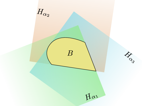
Figure 2. Lemma 12 in the case of $2$ dimensions.

Let $B\subseteq\mathbb{R}^{d}$ be a closed set. Let $S^{d-1}$ be the unit sphere in $\mathbb{R}^{d}$. The map $\Phi_{B}\colon S^{d-1}\to\mathbb{R}$ given by

$$\Phi_{B}(\alpha):=\sup_{x\in B}\langle x,\,\alpha\rangle\in{\mathbb{R}}\cup\{+\infty\}$$

is called the support function of $B$ (here we deviate a little bit from the standard definition where $\Phi_{B}$ is defined on the whole ${\mathbb{R}}^{d}$). The following facts are well known (see e.g. [2, Section 7.2]):

Lemma 12.

• ${\rm Convex\,\,Hull}\,(B)=\bigcap_{\alpha\in S^{d-1}(E)}\{x\in\mathbb{R}^{d}\,|\,\langle x,\alpha\rangle\leqslant\Phi_{B}(\alpha)\}$.

• $\Phi_{B}=\Phi_{{\rm Convex\,\,Hull}\,(B)}$.

Proposition 13.

 

• Let $A$ and $B$ be closed sets. Then we have the following equivalence :

  $$\left(\Phi_{A}\leqslant\Phi_{B}\right)\Longleftrightarrow\left({\rm Convex\,\,Hull}\,\left(A\right)\subset{\rm Convex\,\,Hull}\,\left(B\right)\right).$$

• Let $A$ be a convex closed set. Let $\epsilon>0$. Then

  $$\Phi_{A}+\epsilon\,\,=\,\,\Phi_{A+\overline{{\rm B}(0,\epsilon)}}$$

• Let $B$ be a compact set, and let $C\geqslant 0$ such that for all $x\in B,\quad\|x\|\leqslant C$. Then $\Phi_{B}$ is $C$-Lipschitz.

Proof.

(i) If $\Phi_{A}\leqslant\Phi_{B}$, then Lemma 12(i) gives ${\rm Convex\,\,Hull}\,\left(A\right)\subset{\rm Convex\,\,Hull}\,\left(B\right)$. Conversely, if ${\rm Convex\,\,Hull}\,\left(A\right)\subset{\rm Convex\,\,Hull}\,\left(B\right)$, then by definition of the maps $\Phi$, we have $\Phi_{{\rm Convex\,\,Hull}\,\left(A\right)}\leqslant\Phi_{{\rm Convex\,\,Hull}\,\left(B\right)}$. We conclude by Lemma 12(ii).

(ii) If $x\in A$ and $b\in\overline{{\rm B}(0,\epsilon)}$, we have

$$\langle\alpha,x+b\rangle\leqslant\langle\alpha,x\rangle+\epsilon,$$

and hence $\Phi_{A+\overline{{\rm B}(0,\epsilon)}}\leqslant\Phi_{A}+\epsilon$. Conversely, note that $\epsilon=\langle\alpha,\epsilon\alpha\rangle$. Therefore

(17) $$\langle\alpha,x\rangle+\epsilon = \langle\alpha,x\rangle+\langle\alpha,\epsilon\alpha\rangle$$

$$= \langle\alpha,\underbrace{x+\epsilon\alpha}_{\in A+\overline{{\rm B}(0,\epsilon)}}\rangle$$

$$\leqslant \sup_{x\in A+\overline{{\rm B}(0,\epsilon)}}\langle\alpha,x\rangle$$

which concludes the proof.

(iii) If $\alpha,\alpha^{\prime}\in S^{d-1}$, we have

$$\left|\langle x,\alpha\rangle-\langle x,\alpha^{\prime}\rangle\right|\leqslant\|x\|\|\alpha-\alpha^{\prime}\|,$$

which easily implies

$$|\Phi_{B}(\alpha)-\Phi_{B}(\alpha^{\prime})|\leqslant C\|\alpha-\alpha^{\prime}\|\;.$$

∎

7. Proof of Theorems 7 and 8

Lemma 14.

Let $T_{1},\dots,T_{d}$ be pairwise commuting selfadjoint (possibly unbounded) operators on a Hilbert space. For any $\alpha\in S^{d-1}$, let $\sigma(\alpha)$ be the spectrum of $T^{(\alpha)}:=\sum_{j=1}^{d}\alpha_{j}\,T_{j}$. Then for any fixed $\alpha$,

(18) $$\sup\sigma(\alpha)=\sup\{\langle x,\,\alpha\rangle\,|\,x\in{\rm JointSpec}(T_{1},\ldots,T_{d})\}$$

$$=\sup\{\langle x,\,\alpha\rangle\,|\,x\in{\rm Convex\,\,Hull}\,({\rm JointSpec}(T_{1},\ldots,T_{d}))\}.$$

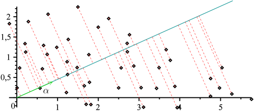
Figure 3. The projection of the joint spectrum onto the line directed by the vector $\alpha$ gives the spectrum of $\sum_{j=1}^{d}\alpha_{j}T_{j}$

Proof.

Let $\mu_{j}$ be the spectral measure of $T_{j}$, and let $\mu=\mu_{1}\otimes\dots\otimes\mu_{d}$ be the joint spectral measure on ${\mathbb{R}}^{d}$. For a given $\alpha\in S^{d-1}$ define a linear functional $\phi:\mathbb{R}^{d}\to\mathbb{R}$ by $\phi(x)=\langle x,\alpha\rangle$. Observe that

$$T^{(\alpha)}=\int_{\mathbb{R}^{d}}\phi\;{\rm d}\mu=\int_{\mathbb{R}}t{\rm d}(\phi_{*}\mu)\;,$$

where $\phi_{*}\mu$ is the push-forward of $\mu$ to $\mathbb{R}$. By definition of the support of a spectral measure, $\phi(\text{supp}(\mu))$ is a dense subset of $\text{supp}(\phi_{*}\mu)$. Thus

$$\{\langle x,\,\alpha\rangle\,|\,x\in{\rm JointSpec}(T_{1},\ldots,T_{d})\}$$

is a dense subset in $\sigma(\alpha)$. This proves the first equality in (18). The second equality follows from Lemma 12(ii). ∎

Now we are ready to give a proof of Theorem 7 and Theorem 8.

Proof of Theorem 7.

We denote by $\Sigma$ the joint spectrum of $(T_{1},\dots,T_{d})$. Let $\alpha\in S^{d-1}\subset{\mathbb{R}}^{d}$ and let $f_{\alpha}:=\langle\alpha,\,F\rangle$. By Lemma 11, we have

$$\lim_{\hbar\to 0}\lambda_{\max}({\rm T}_{f_{\alpha}})=\sup f_{\alpha},$$

which, in view of (18), reads

(19) $$\lim_{\hbar\to 0}\Phi_{\Sigma}(\alpha)=\Phi_{F(M)}(\alpha).$$

Therefore, the map $\Phi_{F(M)}$ can be recovered from the joint spectrum $\Sigma$; by Lemma 12 we can then recover ${\rm Convex\,\,Hull}\,\left(F(M)\right)$, which proves Theorem 7.

Proof of Theorem 8.

If the principal symbols of $T_{1},\dots,T_{d}$ are bounded then the joint spectrum $\Sigma$ is bounded, and it follows from Proposition 13(iii) that the family of maps

$$(\Phi_{\Sigma}-\Phi_{F(M)})_{\hbar\in(0,h_{0}]}$$

is uniformly equicontinuous for $h_{0}>0$ small enough.

This uniform equicontinuity and the compactness of the sphere $S^{d-1}$ imply that the pointwise limit (19) is in fact uniform :

$$\forall\epsilon>0,\exists\hbar_{0}>0,\forall\alpha\in S^{d-1},\forall\hbar<\hbar_{0},\,\,\,\,\left|\Phi_{\Sigma}(\alpha)-\Phi_{F(M)}(\alpha)\right|\leqslant\epsilon.$$

Now Proposition 13(i),(ii) gives the inclusions

$${\rm Convex\,\,Hull}\,\left({\rm JointSpec}(T_{1},\ldots,T_{d})\right)\subset{\rm Convex\,\,Hull}\,\left(F(M)\right)+\overline{{\rm B}(0,\epsilon)}$$

and

$${\rm Convex\,\,Hull}\,\left(F(M)\right)\subset{\rm Convex\,\,Hull}\,\left({\rm JointSpec}(T_{1},\ldots,T_{d})\right)+\overline{{\rm B}(0,\epsilon}).$$

In other words, if $\hbar\leqslant\hbar_{0}$, the Hausdorff distance between the joint spectrum of $(T_{1},\ldots,T_{d})$ and $F(M)$ is less than $\epsilon$, which proves Theorem 8.

8. Berezin-Toeplitz quantization

8.1. Preliminaries

In this section we are concerned with Berezin-Toeplitz operators (simply called in the sequel Toeplitz operators) and quantization of classical systems given by such operators, see Kostant [23], Souriau [33], and Berezin [3], as well as the book [4] by Boutet de Monvel and Guillemin for the corresponding microlocal analysis. Many well known results for pseudodifferential operators are now known for Toeplitz operators, see [5, 18, 6, 25, 10].

Let $(M,\omega)$ be a closed symplectic manifold whose symplectic form represents an integral de Rham cohomology class of $M$ times $2\pi$. In what follows such symplectic manifolds will be called prequantizable. When a prequantizable symplectic manifold $(M,\omega)$ is Kähler with respect to a complex structure $J$, the Berezin-Toeplitz quantization can be given by the following geometric construction. Choose a holomorphic Hermitian line bundle ${\mathcal{L}}$ over $M$ so that the curvature of its (unique) Hermitian connection compatible with the holomorphic structure equals $-{\rm i}\omega$ (the existence of such a ${\mathcal{L}}$ is a well known fact from complex algebraic geometry). For a positive integer $m=1/\hbar$,

(20) $$\mathcal{H}_{\hbar}:=\mathrm{H}^{0}(M,\mathcal{L}^{m})$$

is the space of holomorphic sections of $\mathcal{L}^{m}$.

Since $M$ is compact, $\mathcal{H}_{\hbar}$ is a finite dimensional subspace of the Hilbert space ${\rm L}^{2}(M,\mathcal{L}^{m})$. Here the scalar product is defined by integrating the Hermitian pointwise scalar product of sections against the Liouville measure of $M$. Denote by $\Pi_{\hbar}$ the orthogonal projector of ${\rm L}^{2}(M,\mathcal{L}^{m})$ onto ${\mathcal{H}}_{\hbar}$.

Put ${\mathcal{A}}_{0}=\textup{C}^{\infty}(M)$ and define the quantization map ${\rm Op}_{\hbar}$ by

$${\rm Op}_{\hbar}(f)=\Pi_{\hbar}S_{f},$$

where $S_{f}$ is the operator of multiplication by $f$. Here the Planck constant $\hbar$ runs over the set $I=\{{\textstyle\frac{1}{m}}\;|\;m\in{\mathbb{N}}\}$. The fact that ${\rm Op}_{\hbar}$ is a semiclassical quantization in the sense of Definition 4 is proved in [5].

In what follows we shall use that the Berezin-Toeplitz quantization behaves in a functorial way with respect to direct products of closed Kähler manifolds: Given prequantum bundles $\mathcal{L}_{1}$ and $\mathcal{L}_{2}$ over $M_{1}$ and $M_{2}$ respectively, form a prequantum bundle $\mathcal{L}=p_{1}^{*}\mathcal{L}_{1}\otimes p_{2}^{*}\mathcal{L}_{2}$ over $M:=M_{1}\times M_{2}$, where $p_{i}:M\to M_{i}$ is the natural projection. By a version of Künneth formula [31] ${\rm H}^{0}(M,\mathcal{L})={\rm H}^{0}(M_{1},\mathcal{L}_{1})\otimes{\rm H}^{0}(M_{2},\mathcal{L}_{2})$. For a pair of functions $f^{(i)}\in\textup{C}^{\infty}(M_{i})$, $i=1,2$ define a new function $f\in\textup{C}^{\infty}(M)$ by $f(x_{1},x_{2}):=f^{(1)}(x_{1})f^{(2)}(x_{2})$ One can readily check that

(21) $${\rm Op}_{\hbar}(f)={\rm Op}_{\hbar}(f_{1})\otimes{\rm Op}_{\hbar}(f_{2})\;.$$

If $M$ is a prequantizable closed symplectic (but not necessarily Kähler) manifold, there exist several constructions of semiclassical quantizations of $M$ satisfying Definition 4, see [4, 18, 6, 32, 25].

Now we are ready to present some specific applications of our main results in the context of the Berezin-Toeplitz quantization.

8.2. The case of Hamiltonian torus actions

Assume that $M$ is a prequantizable Kähler manifold endowed with a Hamiltonian ${\mathbb{T}}^{d}$-action which preserves the complex structure. Then the Kostant-Souriau formula yields commuting Toeplitz operators whose principal symbols are the components of the ${\mathbb{T}}^{d}$-momentum map. A proof when $d=n$ was outlined in Charles-Pelayo-Vũ Ngọc [12, Theorem 1.4] as a byproduct of the main result of the paper (a normal form theorem for quantum toric systems); the $d\leqslant n$ case was stated in Charles [11, section 3] without further details. Therefore such a quantum ${\mathbb{T}}^{d}$ action, $d\leqslant n$, satisfies the hypothesis of our main theorem.

Not all symplectic manifolds have a complex structure or a prequantum bundle. However a symplectic toric manifold, that is when $2d=2n$ is the dimension of $M$, always admits a compatible complex structure, which is not unique. Furthermore a symplectic toric manifold $M$ with momentum map $\mu:M\to\mathbb{R}^{n}$ is prequantizable if and only if there exists $c\in\mathbb{R}^{n}$ such that the vertices of the polytope $\mu(M)+c$ belong to $2\pi\mathbb{Z}^{n}$. If it is the case, the prequantum bundle is unique up to isomorphism. Figure 1 shows the joint spectrum of a 4-dimensional toric manifold (a Hirzebruch surface).

By the Atiyah and Guillemin-Sternberg theorem [1, 20] , for any Hamiltonian torus action on a connected closed manifold, the image of the momentum map is a rational convex polytope [1, 20]. So the map $\mu=(\mu_{1},\dots,\mu_{n}):M\to\mathbb{R}^{n}$ satisfies the assumption of Corollary 10. Even more, for a symplectic toric manifold, the momentum polytope $\Delta\subset{\mathbb{R}}^{n}$ has the additional property that for each vertex $v$ of $\Delta$, the primitive normal vectors to the facets meeting at $v$ form a basis of the integral lattice ${\mathbb{Z}}^{n}$. We call such a polytope a Delzant polytope.

Definition 15. Two symplectic toric manifolds $(M,\omega,\mu)$ and $(M^{\prime},\omega^{\prime},\mu^{\prime})$ are isomorphic if there exists a symplectomorphism $\varphi:M\rightarrow M^{\prime}$ such that $\varphi^{*}\mu^{\prime}=\mu.$

By the Delzant classification theorem [16], a symplectic toric manifold is determined up to isomorphism by its momentum polytope. Furthemore, for any Delzant polytope $\Delta$, Delzant constructed in [16] a symplectic toric manifold $(M_{\Delta},\omega_{\Delta},\mu_{\Delta})$ with momentum polytope $\Delta$.

Corollary 16 (Isospectrality for toric systems, [12]).

Let $T_{1},\dots,T_{n}$ be commuting self-adjoint Toeplitz operators on a symplectic toric manifold $(M,\,\omega,\,\mu:M\rightarrow{\mathbb{R}}^{n})$ whose principal symbols are the components of $\mu$. Then

$$\Delta:=\lim_{\hbar\rightarrow 0}\textup{JointSpec}(T_{1},\dots,T_{n})$$

is the Delzant polytope $\mu(M)$. Moreover, $(M,\omega,\mu)$ is isomorphic with $(M_{\Delta},\omega_{\Delta},\mu_{\Delta})$.

The approach of the present paper bypasses the precise description of the semiclassical spectral theory, so it is less informative than the one of [12]. However, it has the advantage of concluding isospectrality with an easier proof, which moreover applies in a much more general setting.

8.3. Coupled angular momenta

Here we present an example of a non-toric integrable system modeling a pair of coupled angular momenta as a prequantum bundle of $(S^{2},\frac{1}{2}\sigma)$. It has been described first by D.A. Sadovskií and B.I. Zhilinskií in [30] (see also [34, Example 6.2] and [27, 28] for further discussion).

In order to present this system we need some preliminaries. Consider the unit sphere $S^{2}\subset{\mathbb{R}}^{3}$ equipped with the standard area form $\sigma$ of total area $4\pi$. Let $(x,y,z)$ be the Euclidean coordinates on ${\mathbb{R}}^{3}$ considered as functions on $S^{2}$. The Poisson brackets of these functions satisfy the relation

(22) $$\{x,y\}=z$$

and its cyclic permutations.

Identify $S^{2}$ with the complex projective line $\mathbb{C}P^{1}=\mathbb{C}\cup\{\infty\}$ by the map

$$W\in\mathbb{C}\cup\{\infty\}\mapsto\Big{(}\frac{2\text{Re}\;W}{1+|W|^{2}},\frac{2\text{Im}\;W}{1+|W|^{2}},\frac{1-|W|^{2}}{1+|W|^{2}}\Big{)}\in S^{2}\;.$$

Let $\mathcal{L}$ be the holomorphic line bundle over $\mathbb{C}P^{1}$ dual to the tautological one. We fix the scheme $T$ of the Berezin-Toeplitz quantization associated to $\mathcal{L}$ considered as a prequantum bundle of $(S^{2},\frac{1}{2}\sigma)$. By a straightforward but cumbersome calculation with Berezin’s coherent states [3] one can verify the quantum commutation relation

(23) $$[T_{m}(x),T_{m}(y)]=-\frac{2i}{m+2}T_{m}(z)$$

and its cyclic permutations.

For a positive number $a$, the sphere $(S^{2},a\sigma)$ serves as the phase space of classical angular momentum whose components are given by $(ax,ay,az)$. The number $a$ plays the role of the amplitude of the angular momentum. In view of (22) we have the relation

(24) $$\{x,y\}_{a}=a^{-1}z$$

and its cyclic permutations, where $\{.,.\}_{a}$ stands for the Poisson bracket associated to $a\sigma$. If $a$ is a positive half-integer, that is $a\in\mathbb{N}/2$, the sphere $(S^{2},a\sigma)$ is quantizable with the prequantum bundle $\mathcal{L}^{2a}$. The corresponding Berezin-Toeplitz quantization $T^{(a)}$ is given by

(25) $$T_{m}^{(a)}(f)=T_{2am}(f)\;.$$

Fix now $a_{1},a_{2}>0$. The phase space of the system of coupled angular momenta is the manifold $M=S^{2}\times S^{2}$ equipped with the symplectic form $\omega=a_{1}\sigma_{1}\oplus a_{2}\sigma_{2}$, while the coupling Hamiltonian is independent on $a_{1},a_{2}$ and is given by

$$H=x_{1}x_{2}+y_{1}y_{2}+z_{1}z_{2}.$$

Here and below we equip all the data corresponding to the first and the second factor of $M$ by lower indices $1$ and $2$ (e.g. $x_{2}$ is the $x$-coordinate on the second factor, etc.) We write $\{.,.\}_{M}$ for the Poisson bracket on $M$. The coupling Hamiltonian $H$ admits a first integral $F=a_{1}z_{1}+a_{2}z_{2}$. Indeed, by using (24) one readily checks that $\{H,F\}_{M}=0$.

In order to quantize this system, introduce the prequantum bundle $L=p_{1}^{*}\mathcal{L}_{1}^{2a_{1}}\otimes p_{2}^{*}\mathcal{L}_{2}^{2a_{2}}$ over $M$, where $\mathcal{L}_{j}$ is a copy of $\mathcal{L}$ over the $j$-th factor of $M$, and $p_{j}$ is the projection of $M$ to the $j$-th factor, $j=1,2$. Denote by $\widehat{T}_{m}$ the corresponding Berezin-Toeplitz quantization.

For $j=1,2$ put $\gamma_{j,m}:=1+a_{j}^{-1}m^{-1}$, and set

$$X_{j} := \gamma_{j,m}\widehat{T}_{m}(x_{j}),$$

$$Y_{j} := \gamma_{j,m}\widehat{T}_{m}(y_{j}),$$

$$Z_{j} := \gamma_{j,m}\widehat{T}_{m}(z_{j})\;.$$

By (21) and (25), the operators

$$\widehat{H}_{m}:=X_{1}\otimes X_{2}+Y_{1}\otimes Y_{2}+Z_{1}\otimes Z_{2}$$

and

$$\widehat{F}_{m}:=a_{1}Z_{1}\otimes{{\rm Id}}+{{\rm Id}}\otimes a_{2}Z_{2}$$

are Toeplitz operators with the principal symbols $H$ and $F$ respectively. The commutation relations (23) readily yield that $[\widehat{H},\widehat{F}]=0$. Let us emphasize that for a given integrable system $F_{1},\dots,F_{n}$, the existence of pair-wise commuting semiclassical operators with principal symbols $F_{1},\dots,F_{n}$ is not at all automatic, see [12] for a discussion and references.

Next, let us describe the classical spectrum of the system, that is the image of the momentum map

$$\Phi:S^{2}\times S^{2}\to\mathbb{R}^{2},\;(v,w)\mapsto(F(v,w),H(v,w))\;.$$

Without loss of generality assume that $a_{1}=1$ and $a_{2}=a\geqslant 1$ (otherwise make a rescaling, maybe after the permutation of the variables). It is not hard to see that the image of the map

$$\Psi:S^{2}\times S^{2}\to\mathbb{R}^{3},\;(v,w)\mapsto v+aw$$

is the spherical shell

$$\{u\in{\mathbb{R}}^{3}\;:\;a-1\leqslant|u|\leqslant a+1\}\;.$$

Observe that

$$H=\frac{1}{2a}\cdot(|\Psi|^{2}-a^{2}-1)\;,$$

and $F$ is simply the $z$-coordinate of $\Psi$. Therefore on each sphere of radius

$$r:=|\Psi|=\sqrt{1+a^{2}+2aH}\in[a-1,a+1]\;,$$

in $\mathbb{R}^{3}$ centered at the origin, the value of $F$ runs from $-r$ to $r$. Furthermore, $H$ is an increasing function of $r$ which takes values $\pm 1$ at $r=a\pm 1$. We conclude that the image of $\Phi=(F,H)$ is the domain $\Delta\subset\mathbb{R}^{2}$ given by the inequalities

$$F^{2}\leqslant 1+a^{2}+2aH,\;\;-1\leqslant H\leqslant 1\;.$$

This domain is clearly convex.

We conclude by Theorem 1 that the convex hull of the joint spectrum of the Toeplitz operators $\widehat{F}_{m}$ and $\widehat{H}_{m}$ converges to $\Delta$ in the Hausdorff sense as $m\to\infty$.

9. $\hbar$-Pseudodifferential quantization

9.1. Preliminaries

If $M={\mathbb{R}}^{2n}$ or $M$ is the cotangent bundle of a closed manifold, then a well-known semiclassical quantization of $M$ is given by $\hbar$-pseudodifferential operators, which is a semiclassical variant of the standard homogeneous pseudodifferential operators (see for instance [17]). In this setting, commuting semiclassical pseudodifferential operators have been considered by Charbonnel [8]; see also [35]. In the remaining of this text, we omit the $\hbar-$ prefix for notational simplicity.

Symbolic calculus of pseudodifferential operators is known to hold when the symbols belong to a Hörmander class. For instance one can take

$$\mathcal{A}_{0}:=\{f\in\textup{C}^{\infty}({\mathbb{R}}^{2n}_{(x,\xi)})\,\,:\,\,\exists m\in{\mathbb{R}}\quad\left|\partial_{(x,\xi)}^{\alpha}f\right|\leqslant C_{\alpha}\langle(x,\xi)\rangle^{m}\quad\forall\alpha\in{\mathbb{N}}^{2n}\}.$$

Here $\langle z\rangle:=(1+|z|^{2})^{1/2}$ for $z\in{\mathbb{R}}^{q}$. If $f\in\mathcal{A}_{0}$, its Weyl quantization is defined on $\mathcal{S}({\mathbb{R}}^{n})$ by

(26) $$({\rm Op}_{\hbar}(f)u)(x):=\frac{1}{(2\pi\hbar)^{n}}\int_{{\mathbb{R}}^{2n}}\textup{e}^{\frac{\textup{i}}{\hbar}((x-y)\cdot\xi)}f({\textstyle\frac{x+y}{2}},\xi)u(y)\textup{d}y\textup{d}\xi.$$

Let $X$ be a closed $n$-dimensional manifold equipped with a smooth density $\mu$. We cover it by a finite set of coordinate charts $U_{1},\dots,U_{N}$ each of which is identified with a convex bounded domain of ${\mathbb{R}}^{n}$ equipped with the Lebesgue measure (the existence of such an atlas readily follows from Moser’s argument [15]). Let $\chi_{1}^{2},\dots,\chi_{N}^{2}$ be a partition of unity subordinated to $U_{1},\dots,U_{N}$, that is $\text{supp}(\chi_{j})\subset U_{j}$ and

$$\sum_{j}\chi_{j}^{2}=1.$$

Then, for any $f\in\textup{C}^{\infty}(\textup{T}^{*}X)$ such that

$$\left|\partial_{\xi}^{\alpha}f(x)\right|\leqslant C_{\alpha}\langle\xi\rangle^{m},\qquad\forall(x,\xi)\in\textup{T}^{*}X,\;\forall\alpha\in{\mathbb{N}}^{n},$$

for some $m\in{\mathbb{R}}$, we define, for $u\in\textup{C}^{\infty}(X)$,

(27) $${\rm Op}_{\hbar}(f)u:=\sum_{j=1}^{N}\chi_{j}\cdot{\rm Op}_{\hbar}^{j}(f)(\chi_{j}u)\;,$$

where ${\rm Op}_{\hbar}^{j}(f)$ is the Weyl quantization calculated in $U_{j}$. The operator $u\mapsto\chi_{j}\cdot{\rm Op}_{\hbar}^{j}(f)(\chi_{j}u)$ is a pseudodifferential operator on $X$ with principal symbol $f(x,\xi)\chi_{j}^{2}(x)$ for $(x,\xi)\in\textup{T}^{*}_{x}X$. Therefore ${\rm Op}_{\hbar}(f)$ is a pseudodifferential operator on $X$ with principal symbol $\sum f\chi_{j}^{2}=f$. The standard pseudodifferential symbolic calculus [17, 37] gives the following proposition.

Proposition 17.

$\hbar$-pseudodifferential quantization on $X$, where $X$ is either ${\mathbb{R}}^{n}$ or a closed manifold equipped with a density, is a semiclassical quantization of $\textup{T}^{*}X$ in the sense of Definition 4, where $\mathcal{A}_{0}$ is a Hörmander symbol class, $I=(0,1]$, the Hilbert space $\mathcal{H}_{\hbar}$ is $\textup{L}^{2}(X)$ (it is independent of $\hbar$). If $X={\mathbb{R}}^{n}$, ${\rm Op}_{\hbar}(f)$ is given by the Weyl quantization. If $X$ is a closed manifold, ${\rm Op}_{\hbar}(f)$ is constructed via formula (27).

Proof.

For the reader’s convenience, let us outline the proof of the proposition. Let $S_{j}:\textup{C}^{\infty}(U_{j})\to\textup{C}^{\infty}_{0}(U_{j})$ be the operator of multiplication by $\chi_{j}$. Then (27) reads ${\rm Op}_{\hbar}(f)=\sum_{j}S_{j}{\rm Op}_{\hbar}^{j}(f)S_{j}$, and so ${\rm Op}_{\hbar}(f)$ is self-adjoint since $S_{j}$ and the Weyl quantization are self-adjoint. Axiom (Q1) follows from the fact that $S_{j}{\rm Op}_{\hbar}^{j}(1)S_{j}=S_{j}^{2}$, and $\sum_{j}S_{j}^{2}={\rm Id}$. Axiom (Q2) is known as the Gårding inequality [17, Theorem 7.12]. Axiom (Q4) is a consequence of the product formula for the Weyl quantization (see e.g. [17, Theorem 7.9]).

For property (Q3) see [37, Theorem 13.13]. Alternatively, it is not hard to derive it from a standard result on spectral asymptotics for $\hbar$-pseudo-differential operators (see e.g. [17, Corollary 9.7]). For reader’s convenience, we present a direct short argument.

Let $P$ be a pseudo-differential operator with a compactly supported principal symbol $p\neq 0$. Take $(x_{0},\xi_{0})\in{\rm T}^{*}X$ such that $p(x_{0},\xi_{0})\neq 0$. Let $\chi$ be a smooth function on $X$ supported in a small neigbourhood of $x_{0}$, contained in a coordinate chart $U$ for $X$, and such that $\|\chi\|_{L^{2}(X)}=1$. In these coordinates, we define the WKB function on $U$

(28) $$u_{\hbar}(x):={\rm e}^{\frac{{\rm i}}{\hbar}\langle x,\xi_{0}\rangle}\chi(x).$$

Then we may compute directly

$$(\chi Pu_{\hbar})(x)=\frac{1}{(2\pi\hbar)^{n}}\int_{\mathbb{R}^{2n}}{\rm e}^{\frac{{\rm i}}{\hbar}\langle x-y,\xi\rangle}a_{\hbar}({\textstyle\frac{x+y}{2}},\xi){\rm e}^{\frac{{\rm i}}{\hbar}\langle y,\xi_{0}\rangle}\chi(y)\chi(x){\rm d}y{\rm d}\xi.$$

The phase

$$\varphi(x,y,\xi)=\langle x-y,\xi\rangle+\langle y,\xi_{0}\rangle$$

is stationary when $\partial_{y}\varphi=\xi_{0}-\xi=0$ and $\partial_{\xi}\varphi=x-y=0$. The hessian

$${\rm d}^{2}\varphi=\begin{pmatrix}0&-{\rm Id}\\ -{\rm Id}&0\end{pmatrix}$$

is non-degenerate. Thus, for fixed $x$ in a neighborhood $V$ of $x_{0}$ the stationary phase approximation gives

$$\left|(\chi Pu_{\hbar})(x)\right|=\left|a_{\hbar}(x,\xi_{0})\chi(x)\right|+\mathcal{O}(\hbar)=\left|p(x,\xi_{0})\chi(x)\right|+\mathcal{O}(\hbar).$$

Hence

(29) $$\left|Pu_{\hbar}(x)\right|=\left|p(x,\xi_{0})\right|+\mathcal{O}(\hbar).$$

Furthermore, the remainder in (29) is of order $\mathcal{O}(\hbar)$ uniformly in $x\in V$. Therefore, shrinking the neighborhood $V$ if necessary, we get that

$$\forall x\in V,\qquad\left|Pu_{\hbar}(x)\right|>\left|p(x_{0},\xi_{0})\right|/2$$

for $\hbar$ small enough. This gives the desired result, since

$$\|P\|\geqslant\|Pu_{\hbar}\|_{{\rm L}^{2}(X)}\geqslant\left|p(x_{0},\xi_{0})\right|\sqrt{\text{Volume}{V}}/2.$$

This completes the proof. ∎

Remark 18. In Theorem 2(ii) and Corollary 3 the assumption on mild dependence of the symbol on $\hbar$ cannot be dropped. Indeed, consider a single $\hbar$-pseudodifferential operator ${\rm Op}_{\hbar}(\hbar x)=\hbar x$ on $\mathbb{R}$. Here the dependence of $a(x,\xi,\hbar)=\hbar x$ on $\hbar$ is not mild. The principal symbol vanishes so the classical spectrum equals $\{0\}$, while for each $\hbar>0$ the spectrum of ${\rm Op}_{\hbar}(\hbar x)$ equals $\mathbb{R}$. We conclude that the classical spectrum cannot be recovered from the quantum one in the classical limit. Let us mention that the formulation and the proof of Theorem 7 remain valid if we allow a slightly more general class of symbols

$$a(x,\xi,\hbar)=a_{0}(x,\xi)+\hbar a_{1,\hbar}(x,\xi)\;,$$

where all $a_{1,\hbar}(x,\xi)$ are uniformly (in $\hbar$) bounded but not necessarily compactly supported. The significance of such a generalization is questionable since such symbols do not form an algebra. It contains however two subspaces that are algebras: ${\mathcal{A}}_{I}$ as defined in the present paper, and ${\mathcal{A}}^{\prime}_{I}$ which is defined by requesting $a_{0}$ to be bounded and $a_{1,\hbar}$ to be uniformly bounded. $\oslash$

9.2. Example: particle in a rotationally symmetric potential

Consider a particle on the plane $\mathbb{R}^{2}(x_{1},x_{2})$ with potential energy $V(x_{1}^{2}+x_{2}^{2})$, where $V$ is a smooth function on $[0,+\infty)$ such that $V(0)=0$, $V>0,V^{\prime}>0$ and $V^{\prime\prime}\geqslant 0$ on $(0,+\infty)$.

The Hamiltonian of the particle is

$$H(x,\xi)=\frac{\xi_{1}^{2}+\xi_{2}^{2}}{2}+V(x_{1}^{2}+x_{2}^{2}).$$

The corresponding Hamiltonian system admits a first integral, the angular momentum $F(x,\xi)=x_{1}\xi_{2}-x_{2}\xi_{1}\;$. Fix a Hörmander class ${\mathcal{A}}_{0}$ and assume that it contains $H$. A standard calculation with the Weyl quantization shows that

$${\rm Op}_{\hbar}(H) = -\frac{1}{2}\hbar^{2}\cdot\Big{(}\frac{\partial^{2}}{\partial x_{1}^{2}}+\frac{\partial^{2}}{\partial x_{2}^{2}}\Big{)}+V(x_{1}^{2}+x_{2}^{2})\;;$$

$${\rm Op}_{\hbar}(F) = -{\rm i}\hbar\Big{(}x_{1}\cdot\frac{\partial}{\partial x_{2}}-x_{2}\cdot\frac{\partial}{\partial x_{1}}\Big{)}\;.$$

The operators ${\rm Op}_{\hbar}(H),{\rm Op}_{\hbar}(G)$ commute.

Lemma 19.

Let

(30) $$g(z):=\max_{r\geqslant 0}(rz-rV(r))$$

be the Legendre transform of $rV(r)$. Then $g(0)=0$, $g>0$ on $(0,+\infty)$, and $\sqrt{g}$ is concave on $(0,+\infty)$.

Proof.

It is immediate that $g(0)=0$ and $g>0$ on $(0,+\infty)$. Now assume $z>0$. The maximum of $rz-rV(r)$ is attained at a unique point, say $r(z)$. By a property of the Legendre transform,

(31) $$g^{\prime}(z)=r(z)\;,$$

and hence

(32) $$g^{\prime\prime}(z)=r^{\prime}(z)\;.$$

Observe also that $r^{\prime}>0$: indeed, $g$ is strictly convex since $rV$ is strictly convex on $(0,+\infty)$. Further,

(33) $$z=(rV)^{\prime}(r(z))=r(z)V^{\prime}(r(z))+V(r(z))\;.$$

Differentiating by $z$ we get that

(34) $$1=2r^{\prime}(z)V^{\prime}(r(z))+r(z)r^{\prime}(z)V^{\prime\prime}(r(z))\geqslant 2r^{\prime}(z)V^{\prime}(z)\;,$$

where the last inequality follows from $V^{\prime\prime}\geqslant 0$. By (33),

(35) $$g(z)=r(z)(z-V(r(z))=r^{2}(z)V^{\prime}(r(z))\;.$$

In order to prove concavity of $\sqrt{g}$ it suffices to check that $(\sqrt{g})^{\prime\prime}\leqslant 0$, that is $(g^{\prime})^{2}\geqslant 2gg^{\prime\prime}\;$. By (31),(32) and (35) this is equivalent to $r^{2}(z)\geqslant 2r^{2}(z)V^{\prime}(r(z))r^{\prime}(z)$, but this follows from equation (34). ∎

Proposition 20.

Assume that $V(0)=0$ and $V>0,V^{\prime}>0$ and $V^{\prime\prime}\geqslant 0$ on $(0,+\infty)$. Then the classical spectrum of $(({\rm Op}_{\hbar}(H)),({\rm Op}_{\hbar}(F)))$ is convex, and hence by Corollary 3(ii) it can be recovered from the joint spectrum of $({\rm Op}_{\hbar}(H),{\rm Op}_{\hbar}(F))$ in the classical limit.

Proof.

Put $s=\frac{\xi_{1}^{2}+\xi_{2}^{2}}{2}$ and $r=x_{1}^{2}+x_{2}^{2}$. Fix an energy level $\Sigma_{z}=\{H=z\}$, that is $s=z-V(r)$. Let $g(z)$ be the maximal possible value of $rs$ on this level, that is $g$ is given by (30). Let $r(z)$ be as in the lemma above. Since

$$\{|x|=\sqrt{r(z)},\;|\xi|=\sqrt{2(z-V(r(z)))}\}\subset\Sigma_{z},$$

the value of $F(x,\xi)=x_{1}\xi_{2}-x_{2}\xi_{1}$ runs between $-|x|\cdot|\xi|=-\sqrt{2g(z)}$ and $|x|\cdot|\xi|=\sqrt{2g(z)}$. It follows that the classical spectrum is the subset of $\mathbb{R}^{2}$ defined by $|F|\leqslant\sqrt{2g(H)}$, which, by Lemma 19, a is convex set. ∎

10. Non-commuting operators

Let ${\mathcal{H}}$ be a separable Hilbert space, and let $T_{1},\dots,T_{d}$ be possibly unbounded selfadjoint operators on ${\mathcal{H}}$. Denote by ${\mathcal{Q}}$ the set of all mixed quantum states for $T_{1},\dots,T_{d}$ : the elements of ${\mathcal{Q}}$ are trace class selfadjoint operators $Q\in{\mathcal{L}}({\mathcal{H}})$ such that

1. $Q\geqslant 0$;

2. $\mathop{\textup{trace}}{Q}=1$;

3. $T_{j}Q\in{\mathcal{L}}^{1}$, for all $j=1,\dots,d$.

Here ${\mathcal{L}}^{1}$ stands for the Schatten trace class, and the image of $Q$ is assumed to lie in the domain of $T_{j}$, $j=1,\ldots,d$. Of course ${\mathcal{Q}}$ is not a vector space, but it is a convex set of compact operators. The third condition is void in case the operators $T_{j}$’s are bounded: indeed, the Hölder inequality gives

$$\|T_{j}Q\|_{{\mathcal{L}}^{1}}\leqslant\|T_{j}\|\|Q\|_{{\mathcal{L}}^{1}}$$

(see also [29, Theorem VI.19]).

Definition 21. The map

(36) $$E:{\mathcal{Q}}\to{\mathbb{R}}^{d},\;\;Q\mapsto(\mathop{\textup{trace}}(T_{1}Q),\dots,\mathop{\textup{trace}}(T_{d}Q))\;,$$

is called the expectation map. We denote by $\Sigma(T_{1},\dots,T_{d})\subset\mathbb{R}^{d}$ the closure of the image of $E$.

An interesting subset of ${\mathcal{Q}}$ consists of the so-called pure states, i.e. rank-one orthogonal projectors. We shall call the closure of the image of pure states by $E$ the joint numerical range $R$ :

$$R:=\overline{\{(\langle T_{1}u,u\rangle,\dots,\langle T_{d}u,u\rangle);\quad u\in{\mathcal{H}},\|u\|=1\}}\subset\Sigma(T_{1},\dots,T_{d}).$$

Lemma 22.

$\Sigma(T_{1},\dots,T_{d})$ is the convex hull of $R$.

Proof.

Let $Q\in{\mathcal{Q}}$, and let $(e_{n})_{n\geqslant 0}$ be a Hilbert basis of eigenvectors of $Q$ so that $Qe_{n}=q_{n}e_{n}$. For any $j=1,\dots,d$, we can write

$$\mathop{\textup{trace}}{T_{j}Q}=\sum_{n\geqslant 0}\langle T_{j}Qe_{n},e_{n}\rangle=\sum_{n\geqslant 0}q_{n}\langle T_{j}e_{n},e_{n}\rangle,$$

where $q_{n}\geqslant 0$ and $\sum_{n}q_{n}=1$. Therefore any element of $E({\mathcal{Q}})$ is of the form $\sum_{n}q_{n}\vec{z}_{n}$, where

$$\vec{z}_{n}:=(\langle T_{1}e_{n},e_{n}\rangle,\dots\langle T_{d}e_{n},e_{n}\rangle)\in R.$$

Being an infinite convex combination of elements of $R$, $\vec{z}_{n}$ must lie in the closed convex hull of $R$, which is equal to the convex hull of $R$ since $R$ is closed, by definition. Thus

$$\Sigma(T_{1},\dots,T_{d})\subset{\rm Convex\,\,Hull}\,\left(R\right).$$

The other inclusion follows from $R\subset\Sigma(T_{1},\dots,T_{d})$ and the fact that, since ${\mathcal{Q}}$ is a convex set and $E$ is an affine map, $\Sigma(T_{1},\ldots,T_{d})$ is convex. ∎

Proposition 23.

If the operators $T_{1},\dots,T_{d}$ pairwise commute, the set $\Sigma(T_{1},\dots,T_{d})$ coincides with ${\rm Convex\,\,Hull}\,(\textup{JointSpec}(T_{1},\dots,T_{d}))$.

Proof.

Using the notation of Section 6, we consider the map $\alpha\mapsto\Phi_{R}(\alpha)$, $\alpha\in S^{d-1}$. Notice that

(37) $$\Phi_{R}(\alpha)=\sup_{\|u\|=1}\langle T^{(\alpha)}u,u\rangle,$$

where $T^{(\alpha)}:=\sum_{j}\alpha_{j}T_{j}$. From Lemma 14, we have

(38) $$\sup_{\|u\|=1}\langle T^{(\alpha)}u,u\rangle=\Phi_{\!\!\mathop{\rm~{}JointSpec}\nolimits(T_{1},\dots,T_{d})}(\alpha).$$

Therefore, by Lemma 12,

$${\rm Convex\,\,Hull}\,\left(R\right)={\rm Convex\,\,Hull}\,\left(\!\!\mathop{\rm~{}JointSpec}\nolimits(T_{1},\dots,T_{d})\right).$$

The result now follows from Lemma 22. ∎

Remark 24. Proposition 23 applied to one operator $T$ with spectrum $\sigma$ gives $\max\sigma(T)=\max\Sigma(T)$. $\oslash$

The following extends Theorem 1.

Theorem 25.

If $\{T_{j,\hbar}\}$ is any collection of semiclassical operators and classical spectrum $\mathcal{S}$. Let $J$ be a subset of $I$ that accumulates at $0$. Then:

• From the family

  $$\Big{\{}{\rm Convex\,\,Hull}\,\Big{(}\textup{JointSpec}(T_{1},\dots,T_{d})\Big{)}\Big{\}}_{\hbar\in J}$$

  one can recover the convex hull of $\mathcal{S}$;

• If moreover the principal symbols of $T_{1},\ldots,T_{d}$ are bounded then

  $$\lim_{\hbar\rightarrow 0}\Sigma(T_{1,\hbar},\dots,T_{d,\hbar})\,=\,{\rm Convex\,\,Hull}\,\left(\mathcal{S}\right).$$

Proof.

Recall from (37) and (38) that if $\alpha\in S^{d-1}$,

(39) $$\max\sigma\Big{(}\sum_{j=1}^{d}\alpha_{j}T_{j}\Big{)}=\max\{\langle x,\alpha\rangle\,\,|\,\,x\in\Sigma(T_{1},\dots,T_{d})\}\;.$$

Now we repeat the proof of Theorem 7. Let $F$ be the map of principal symbols of $T_{1},\dots,T_{d}$, and write $f_{\alpha}:=\langle\alpha,\,F\rangle$. By Lemma 11, we have that

$$\lim_{\hbar\to 0}\max\sigma\Big{(}\sum_{j=1}^{d}\alpha_{j}T_{j}\Big{)}=\max f_{\alpha}$$

which, in view of (39), reads

(40) $$\lim_{\hbar\to 0}\Phi_{\Sigma(T_{1},\dots,T_{d})}(\alpha)=\Phi_{F(M)}(\alpha).$$

To finish the proof we repeat the proof of Theorem 8, where the convex hull ${\rm Convex\,\,Hull}\,(\textup{JointSpec}(T_{1},\dots,T_{d}))$ is replaced by $\Sigma(T_{1},\dots,T_{d})$, and (19) by (40). ∎

Acknowledgements. AP was partially supported by NSF Grants DMS-0965738 and DMS-0635607, an NSF CAREER Award, a Leibniz Fellowship, Spanish Ministry of Science Grants MTM 2010-21186-C02-01 and Sev-2011-0087. LP is partially supported by the National Science Foundation grant DMS-1006610 and the Israel Science Foundation grant 509/07. He gratefully acknowledges the warm hospitality from the University of Chicago where part of this project has been fulfilled. VNS is partially supported by the Institut Universitaire de France, the Lebesgue Center (ANR Labex LEBESGUE), and the ANR NOSEVOL grant. He gratefully acknowledges the hospitality of the IAS.

Álvaro Pelayo
School of Mathematics
Institute for Advanced Study
Einstein Drive
Princeton, NJ 08540 USA.

Washington University, Mathematics Department
One Brookings Drive, Campus Box 1146
St Louis, MO 63130-4899, USA.
E-mail: apelayo@math.wustl.edu
Website: http://www.math.wustl.edu/~apelayo/

Leonid Polterovich
School of Mathematical Sciences
Tel Aviv University
69978 Tel Aviv
Israel
E-mail: polterov@runbox.com
Website: http://www.math.tau.ac.il/~polterov/

San Vũ Ngọc
Institut Universitaire de France

Institut de Recherches Mathématiques de Rennes
Université de Rennes 1
Campus de Beaulieu
F-35042 Rennes cedex, France
E-mail: san.vu-ngoc@univ-rennes1.fr
Website: http://blogperso.univ-rennes1.fr/san.vu-ngoc/

References

• [1] Atiyah, M.: Convexity and commuting Hamiltonians, Bull. London Math. Soc. 14 (1982) 1–15.
• [2] H.H. Bauschke and P.L. Combettes: Convex analysis and monotone operator theory in Hilbert spaces, Springer, New York, 2011.
• [3] F.A. Berezin: General concept of quantization, Comm. Math. Phys., 40 153-174.
• [4] L. Boutet de Monvel and V. Guillemin. The Spectral Theory of Toeplitz operators, Annals of Mathematics Studies 99. Princeton University Press, Princeton, NJ, 1981.
• [5] M. Bordemann, E. Meinrenken, and M. Schlichenmaier: Toeplitz quantization of Kähler manifolds and $gl(N),N\to\infty$ limits, Comm. Math. Phys. 165 (1994) 281-296.
• [6] D. Borthwick and A. Uribe: Almost complex structures and geometric quantization, Math. Res. Lett. 3 (1996), 845-861.
• [7] D. Burago, Y. Burago, and S. Ivanov: A Course in Metric Geometry, Graduate Studies in Mathematics, 33. American Mathematical Society, Providence, RI, 2001.
• [8] A.-M. Charbonnel: Comportement semi-classique du spectre conjoint d’opérateurs pseudodifférentiels qui commutent. Asymptotic Anal. 1 (1988), no. 3, 227–261.
• [9] L.Charles: Berezin-Toeplitz operators, a semi-classical approach, Comm. Math. Phys. 239 (2003) 1-28.
• [10] L. Charles: Quasimodes and Bohr-Sommerfeld conditions for the Toeplitz operators. Comm. Partial Differential Equations, 28(9-10) (2003) 1527-1566.
• [11] L. Charles: Toeplitz operators and Hamiltonian Torus Actions, Journal of Functional Analysis 236 (2006) 299-350.
• [12] L. Charles, Á. Pelayo, and S. Vũ Ngọc: Isospectrality for quantum toric integrable systems, arXiv:1111.5985. Accepted to Ann. Sci. École Norm. Sup.
• [13] Y. Colin de Verdière: Spectre conjoint d’opérateurs pseudo-différentiels qui commutent. II. Le cas intégrable, Math. Z. 171 (1980) 51–73.
• [14] Y. Colin de Verdière: Spectre conjoint d’opérateurs pseudo-différentiels qui commutent. I. Le cas non intégrable, Duke Math. J. 46 (1979) 169–182.
• [15] B. Dacorogna and J. Moser, On a partial differential equation involving the Jacobian determinant, Ann. Inst. H. Poincaré Anal. Non Linéaire 7 (1990), 1–-26.
• [16] T. Delzant: Hamiltoniens périodiques et images convexes de l’application moment, Bull. Soc. Math. France 116 (1988) 315–339.
• [17] M. Dimassi and J. Sjöstrand: Spectral asymptotics in the semi-classical limit. London Mathematical Society Lecture Note Series, 268. Cambridge University Press, Cambridge, 1999.
• [18] V. Guillemin: Star products on compact pre-quantizable symplectic manifolds. Lett. Math. Phys. 35 (1995), no. 1, 85–89.
• [19] V. Guillemin, T. Paul and A. Uribe: “Bottom of the Well” Semi-classical Trace Invariants, Math. Res. Lett. 14 (2007), 711-719.
• [20] V. Guillemin and S. Sternberg: Convexity properties of the moment mapping, Invent. Math., 67 (1982), 491–513.
• [21] H. Hezari and S. Zelditch: Inverse spectral problem for analytic $({\mathbb{Z}}/2{\mathbb{Z}})^{n}$-symmetric domains in ${\mathbb{R}}^{n}$. Geom. Funct. Anal. 20 (2010), no. 1, 160–191.
• [22] P.D. Hislop and I.M. Sigal: Introduction to Spectral Theory, Springer, 1995.
• [23] B. Kostant: Quantization and unitary representations. I. Prequantization. Lectures in modern analysis and applications, III, pp. 87-208. Lecture Notes in Math., Vol. 170, Springer, Berlin, 1970.
• [24] A. Iantchenko, J. Sjöstrand and M. Zworski: Birkhoff normal forms in semi-classical inverse problems, Math. Res. Lett. 9 (2002) 337–362.
• [25] Ma, X., Marinescu, G., Toeplitz operators on symplectic manifolds, J. Geom. Anal. 18 (2008), 565-611.
• [26] J. Niechwiej: Support of the joint spectral measure, J. Austral. Math. Soc. (Series A) 43(1987), 74–80.
• [27] Á. Pelayo and S. Vũ Ngọc: Semitoric integrable systems on symplectic $4$-manifolds, Invent. Math. 177 (2009) 571-597.
• [28] Á. Pelayo and S. Vũ Ngọc: Constructing integrable systems of semitoric type, Acta Math. 206 (2011) 93-125.
• [29] M. Reed and B. Simon: Methods of Modern and Mathematical Physics, I : Functional Analysis, Academic Press, 1980.
• [30] D.A. Sadovskií and B.I. Zhilinskií: Monodromy, diabolic points, and angular momentum coupling. Phys. Lett. A, 256(4):235–244, 1999.
• [31] J.H. Sampson and G.A. Washnitzer: A Künneth formula for coherent algebraic sheaves, Illinois J. Math. 3 (1959), 389–-402.
• [32] B. Shiffman and Z. Zelditch: Asymptotics of almost holomorphic sections of ample line bundles on symplectic manifolds. J. Reine Angew. Math. 544 (2002), 181–222.
• [33] J.-M. Souriau: Structure des Systèmes Dynamiques. Maitrises de mathématiques Dunod, Paris 1970 xxxii+414 pp.
• [34] S. Vũ Ngọc: Moment polytopes for symplectic manifolds with monodromy, Adv. Math. 208(2) (2007), 909–934.
• [35] S. Vũ Ngọc: Bohr-Sommerfeld conditions for integrable systems with critical manifolds of focus-focus type. Comm. Pure Appl. Math. 53 (2000), no. 2, 143–217.
• [36] S. Vũ Ngọc: Symplectic inverse spectral theory for pseudodifferential operators. Geometric Aspects of Analysis and Mechanics Progress in Mathematics Birkhäuser/Springer, New York, 2011, Volume 292, 353-372.
• [37] M. Zworski, Semiclassical Analysis, Amer. Math. Soc., 2012.