SISSA 03/2013/FISI IFIC/13-03
Nonzero $|U_{e3}|$ from Charged Lepton Corrections and the Atmospheric Neutrino Mixing Angle (updated using the results of the global fits of 2013 data )

Abstract

After the successful determination of the reactor neutrino mixing angle $\theta_{13}\cong 0.16\neq 0$, a new feature suggested by the current neutrino oscillation data is a sizeable deviation of the atmospheric neutrino mixing angle $\theta_{23}$ from $\pi/4$. Using the fact that the neutrino mixing matrix $U=U^{\dagger}_{e}U_{\nu}$, where $U_{e}$ and $U_{\nu}$ result from the diagonalisation of the charged lepton and neutrino mass matrices, and assuming that $U_{\nu}$ has a i) bimaximal (BM), ii) tri-bimaximal (TBM) form, or else iii) corresponds to the conservation of the lepton charge $L^{\prime}=L_{e}-L_{\mu}-L_{\tau}$ (LC), we investigate quantitatively what are the minimal forms of $U_{e}$, in terms of angles and phases it contains, that can provide the requisite corrections to $U_{\nu}$ so that $\theta_{13}$, $\theta_{23}$ and the solar neutrino mixing angle $\theta_{12}$ have values compatible with the current data. Two possible orderings of the 12 and the 23 rotations in $U_{e}$, “standard” and “inverse”, are considered. The results we obtain depend strongly on the type of ordering. In the case of “standard” ordering, in particular, the Dirac CP violation phase $\delta$, present in $U$, is predicted to have a value in a narrow interval around i) $\delta\cong\pi$ in the BM (or LC) case, ii) $\delta\cong 3\pi/2$ or $\pi/2$ in the TBM case, the CP conserving values $\delta=0,\pi,2\pi$ being excluded in the TBM case at more than $4\sigma$.

In the addendum we discuss the implications of the latest 2013 data.

1 Introduction

Understanding the origin of the patterns of neutrino masses and mixing, emerging from the neutrino oscillation, ${}^{3}H$ $\beta-$decay, etc. data is one of the most challenging problems in neutrino physics. It is part of the more general fundamental problem in particle physics of understanding the origins of flavour, i.e., of the patterns of the quark, charged lepton and neutrino masses and of the quark and lepton mixing.

At present we have compelling evidence for the existence of mixing of three light massive neutrinos $\nu_{i}$, $i=1,2,3$, in the weak charged lepton current (see, e.g., [1]). The masses $m_{i}$ of the three light neutrinos $\nu_{i}$ do not exceed approximately 1 eV, $m_{i}\mathrel{\hbox to0.0pt{\raise 2.20013pt\hbox{$<$}\hss}{\lower 2.20013pt\hbox{$\sim$}}}1$ eV, i.e., they are much smaller than the masses of the charged leptons and quarks. The three light neutrino mixing we will concentrate on in the present article, is described (to a good approximation) by the Pontecorvo, Maki, Nakagawa, Sakata (PMNS) $3\times 3$ unitary mixing matrix, $U_{\rm PMNS}$. In the widely used standard parametrisation [1], $U_{\rm PMNS}$ is expressed in terms of the solar, atmospheric and reactor neutrino mixing angles $\theta_{12}$, $\theta_{23}$ and $\theta_{13}$, respectively, and one Dirac - $\delta$, and two Majorana [2] - $\alpha_{21}$ and $\alpha_{31}$, CP violation (CPV) phases:

$$U_{\text{PMNS}}\equiv U=V(\theta_{12},\theta_{23},\theta_{13},\delta)\,Q(\alpha_{21},\alpha_{31})\,,$$ (1)

where

$$V=\left(\begin{array}[]{ccc}1&0&0\\ 0&c_{23}&s_{23}\\ 0&-s_{23}&c_{23}\\ \end{array}\right)\left(\begin{array}[]{ccc}c_{13}&0&s_{13}e^{-i\delta}\\ 0&1&0\\ -s_{13}e^{i\delta}&0&c_{13}\\ \end{array}\right)\left(\begin{array}[]{ccc}c_{12}&s_{12}&0\\ -s_{12}&c_{12}&0\\ 0&0&1\\ \end{array}\right)\,,$$ (2)

$$Q=\operatorname{diag}(1,e^{i\alpha_{21}/2},e^{i\alpha_{31}/2})\,,$$ (3)

and we have used the standard notation $c_{ij}\equiv\cos\theta_{ij}$, $s_{ij}\equiv\sin\theta_{ij}$ with $0\leq\theta_{ij}\leq\pi/2$, $0\leq\delta\leq 2\pi$ and, in the case of interest for our analysis, $0\leq\alpha_{j1}\leq 2\pi$, $j=2,3$ (see, however, [3]). If CP invariance holds, we have $\delta=0,\pi$, and [4] $\alpha_{21(31)}=0,\pi$.

The neutrino oscillation data, accumulated over many years, allowed to determine the parameters which drive the solar and atmospheric neutrino oscillations, $\Delta m^{2}_{21}$, $\theta_{12}$ and $|\Delta m^{2}_{31}|\cong|\Delta m^{2}_{32}|$, $\theta_{23}$, with a high precision (see, e.g., [5]).

Furthermore, there were spectacular developments in the last 1.5 years in what concerns the angle $\theta_{13}$ (see, e.g., [1]). They culminated in a high precision determination of $\sin^{2}2\theta_{13}$ in the Daya Bay experiment with reactor $\bar{\nu}_{e}$ [6]:

$$\sin^{2}2\theta_{13}=0.089\pm 0.010\pm 0.005\,.$$ (4)

Similarly the RENO, Double Chooz, and T2K experiments reported, respectively, $4.9\sigma$, $2.9\sigma$ and $3.2\sigma$ evidences for a non-zero value of $\theta_{13}$ [7], compatible with the Daya Bay result. The high precision measurement on $\theta_{13}$ described above and the fact that $\theta_{13}$ turned out to have a relatively large value, have far reaching implications for the program of research in neutrino physics (see, e.g., [1]). After the successful measurement of $\theta_{13}$, the determination of the absolute neutrino mass scale, of the type of the neutrino mass spectrum, of the nature - Dirac or Majorana, of massive neutrinos, as well as getting information about the status of CP violation in the lepton sector, are the most pressing and challenging problems and the highest priority goals of the research in the field of neutrino physics.

A global analysis of the latest neutrino oscillation data presented at the Neutrino 2012 International Conference [5], was performed in [8]. The results on $\sin^{2}\theta_{12}$, $\sin^{2}\theta_{23}$ and $\sin^{2}\theta_{13}$ obtained in [8], which play important role in our further discussion, are given in Table 1.

Parameter	Best fit	$1\sigma$ range	$2\sigma$ range	$3\sigma$ range
$\sin\theta_{13}$	0.155	0.147 - 0.163	0.139 - 0.170	0.130 - 0.177
$\sin^{2}\theta_{12}$	0.307	0.291 - 0.325	0.275 - 0.342	0.259 - 0.359
$\sin^{2}\theta_{23}$ (NH)	0.386	0.365 - 0.410	0.348 - 0.448	0.331 - 0.637
$\sin^{2}\theta_{23}$ (IH)	0.392	0.370 - 0.431	0.353 - 0.484 $\oplus$ 0.543 - 0.641	0.335 - 0.663
$\delta$ (NH)	3.39	2.42 - 4.27	—	—
$\delta$ (IH)	3.42	2.61 - 4.62	—	—

Table 1: Summary of the results of the global fit of the PMNS mixing angles taken from [8] and used in our analysis. The results on the atmospheric neutrino angle $\theta_{23}$ and on the Dirac CPV phase $\delta$ depend on the type of neutrino mass hierarchy. The values of $\sin^{2}\theta_{23}$ and $\delta$ obtained in both the cases of normal hierarchy (NH) and inverted hierarchy (IH) are shown.

An inspection of Table 1 shows that, in addition to the nonzero value of $\theta_{13}$, the new feature which seems to be suggested by the current global neutrino oscillation data is a sizeable deviation of the angle $\theta_{23}$ from the value $\pi/4$. This trend is confirmed by the results of the subsequent analysis of the global neutrino oscillation data performed in [9].

Although $\theta_{13}\neq 0$, $\theta_{23}\neq\pi/4$ and $\theta_{12}\neq\pi/4$, the deviations from these values are small, in fact we have $\sin\theta_{13}\cong 0.16\ll 1$, $\pi/4-\theta_{23}\cong 0.11$ and $\pi/4-\theta_{12}\cong 0.20$, where we have used the relevant best fit values in Table 1. The value of $\theta_{13}$ and the magnitude of deviations of $\theta_{23}$ and $\theta_{12}$ from $\pi/4$ suggest that the observed values of $\theta_{13}$, $\theta_{23}$ and $\theta_{12}$ might originate from certain “symmetry” values which undergo relatively small (perturbative) corrections as a result of the corresponding symmetry breaking. This idea was and continues to be widely explored in attempts to understand the pattern of mixing in the lepton sector (see, e.g., [10, 11, 12, 13, 14, 15, 16, 17]). Given the fact that the PMNS matrix is a product of two unitary matrices,

$$U=U_{e}^{\dagger}\,U_{\nu}\,,$$ (5)

where $U_{e}$ and $U_{\nu}$ result respectively from the diagonalisation of the charged lepton and neutrino mass matrices, it is usually assumed that $U_{\nu}$ has a specific form dictated by a symmetry which fixes the values of the three mixing angles in $U_{\nu}$ that would differ, in general, by perturbative corrections from those measured in the PMNS matrix, while $U_{e}$ (and symmetry breaking effects that we assume to be subleading) provide the requisite corrections. A variety symmetry forms of $U_{\nu}$ have been explored in the literature on the subject (see, e.g., [18]). In the present study we will consider three widely used forms.
i) Tribimaximal Mixing (TBM) [19]:

$$U_{\rm TBM}=\left(\begin{array}[]{ccc}\sqrt{\frac{2}{3}}&\sqrt{\frac{1}{3}}&0\\[5.69046pt] -\sqrt{\frac{1}{6}}&\sqrt{\frac{1}{3}}&\sqrt{\frac{1}{2}}\\[5.69046pt] \sqrt{\frac{1}{6}}&-\sqrt{\frac{1}{3}}&\sqrt{\frac{1}{2}}\end{array}\right)\,;$$ (9)

ii) Bimaximal Mixing (BM) [20]:

$$U_{\rm BM}=\left(\begin{array}[]{ccc}\frac{1}{\sqrt{2}}&\frac{1}{\sqrt{2}}&0\\[8.5359pt] -\frac{1}{2}&\frac{1}{2}&\frac{1}{\sqrt{2}}\\[8.5359pt] \frac{1}{2}&-\frac{1}{2}&\frac{1}{\sqrt{2}}\\[8.5359pt] \end{array}\right)\,;$$ (13)

iii) the form of $U_{\nu}$ resulting from the conservation of the lepton charge $L^{\prime}=L_{e}-L_{\mu}-L_{\tau}$ of the neutrino Majorana mass matrix [21] (LC):

$$U_{\rm LC}=\left(\begin{array}[]{ccc}\frac{1}{\sqrt{2}}&\frac{1}{\sqrt{2}}&0\\[8.5359pt] -\frac{c^{\nu}_{23}}{\sqrt{2}}&\frac{c^{\nu}_{23}}{\sqrt{2}}&s^{\nu}_{23}\\[8.5359pt] \frac{s^{\nu}_{23}}{\sqrt{2}}&-\,\frac{s^{\nu}_{23}}{\sqrt{2}}&c^{\nu}_{23}\\[8.5359pt] \end{array}\right)\,,$$ (17)

where $c^{\nu}_{23}=\cos\theta^{\nu}_{23}$ and $s^{\nu}_{23}=\sin\theta^{\nu}_{23}$.

We will define the assumptions we make on $U_{e}$ and $U_{\nu}$ in full generality in Section 2. Those assumptions allow us to cover, in particular, the case of corrections from $U_{e}$ to the three widely used forms of $U_{\nu}$ indicated above. We would like to notice here that if $U_{e}={\bf 1}$, ${\bf 1}$ being the unity $3\times 3$ matrix, we have:
i) $\theta_{13}=0$ in all three cases of interest of $U_{\nu}$;
ii) $\theta_{23}=\pi/4$, if $U_{\nu}$ coincides with $U_{\rm TBM}$ or $U_{\rm BM}$, while $\theta_{23}$ can have an arbitrary value if $U_{\nu}$ is given by $U_{\rm LC}$;
iii) $\theta_{12}=\pi/4$, for $U_{\nu}=U_{\rm BM}$ or $U_{\rm LC}$, while $\theta_{12}=\sin^{-1}(1/\sqrt{3})$ if $U_{\nu}=U_{\rm TBM}$.
Thus, the matrix $U_{e}$ has to generate corrections
i) leading to $\theta_{13}\neq 0$ compatible with the observations in all three cases of $U_{\nu}$ considered;
ii) leading to the observed deviation of $\theta_{12}$ from $\pi/4$ in the cases of $U_{\nu}=U_{\rm BM}$ or $U_{\rm LC}$.
iii) leading to the sizeable deviation of $\theta_{23}$ from $\pi/4$ for $U_{\nu}=U_{\rm TBM}$ or $U_{\rm BM}$, if it is confirmed by further data that $\sin^{2}\theta_{23}\cong 0.40$.

In the present article we investigate quantitatively what are the “minimal” forms of the matrix $U_{e}$ in terms of the number of angles and phases it contains, that can provide the requisite corrections to $U_{\rm TBM}$, $U_{\rm BM}$ and $U_{\rm LC}$ so that the angles in the resulting PMNS matrix have values which are compatible with those derived from the current global neutrino oscillation data, Table 1. Our work is a natural continuation of the study some of us have done in [15] and earlier in [11, 12, 13, 14].

The paper is organised as follows. In Section 2 we describe the general setup and we introduce the two types of “minimal” charged lepton “rotation” matrix $U_{e}$ we will consider: with “standard” and “inverse” ordering. The two differ by the order in which the 12 and 23 rotations appear in $U_{e}$. In the same Section we derive analytic expressions for the mixing angles and the Dirac phase $\delta$ of the PMNS matrix in terms of the parameters of the charged lepton matrix $U_{e}$ both for the tri-bimaximal and bimaximal (or LC) forms of the neutrino “rotation” matrix $U_{\nu}$. In Sections 3 and 4 we perform a numerical analysis and derive, in particular, the intervals of allowed values at a given C.L. of the neutrino mixing angle parameters $\sin^{2}\theta_{12}$, $\sin^{2}\theta_{23}$ and $\sin^{2}\theta_{13}$, the Dirac phase $\delta$ and the rephasing invariant $J_{CP}$ associated with $\delta$, in the cases of the standard and inverse ordering of the charged lepton corrections. A summary and conclusions are presented in Section 5. Further details are reported in two appendices. In Appendix A we illustrate in detail the parametrisation we use for the standard ordering setup. Finally, in Appendix B we describe the statistical analysis used to obtain the numerical results.

2 General Setup

While neutrino masses and mixings may or may not look anarchical, the hierarchy of charged lepton masses suggests an ordered origin of lepton flavour. Given the wide spectrum of specific theoretical models, which essentially allows to account for any pattern of lepton masses and mixings, we would like to consider here the consequence for lepton mixing of simple, general assumptions on its origin. As we have indicated in the Introduction, we are interested in the possibility that the $\theta_{13}$ mixing angle originates because of the contribution of the charged lepton sector to lepton mixing  [10, 11, 12, 13, 14, 15, 16]. The latter assumption needs a precise definition. In order to give it, let us recall that the PMNS mixing matrix is given by

$$U=U_{e}^{\dagger}U_{\nu},\quad\text{with $U_{e}$, $U_{\nu}$ defined by}\quad\begin{aligned} m_{E}=U^{*}_{e^{c}}m^{\text{diag}}_{E}U^{\dagger}_{e}\\ m_{\nu}=U^{*}_{\nu}m^{\text{diag}}_{\nu}U^{\dagger}_{\nu}\end{aligned},$$ (18)

where $m_{E}$ and $m_{\nu}$ are respectively the charged lepton and neutrino Majorana mass matrices (in a basis assumed to be defined by the unknown physics accounting for their structure) and $m^{\text{diag}}_{E}$ and $m^{\text{diag}}_{\nu}$ are diagonal with positive eigenvalues.

We will assume that the neutrino contribution $U_{\nu}$ to the PMNS matrix $U$ has $U^{\nu}_{13}=0$, so that the PMNS angle $\theta_{13}$ vanishes in the limit in which the charged lepton contribution $U_{e}$ can be neglected, $U_{e}=\mathbf{1}$. This is a prediction of a number of theoretical models. As a consequence, $U_{\nu}$ can be parameterized as

$$U_{\nu}=\Psi_{\nu}R_{23}(\theta_{23}^{\nu})R_{12}(\theta_{12}^{\nu})\Phi_{\nu},$$ (19)

where $R_{ij}(\theta)$ is a rotation by an angle $\theta$ in the $ij$ block and $\Psi_{\nu}$, $\Phi_{\nu}$ are diagonal matrices of phases. We will in particular consider specific values of $\theta^{\nu}_{12}$ and, in certain cases, of $\theta^{\nu}_{23}$, representing the predictions of well known models.

The above assumption on the structure of $U_{\nu}$ is not enough to draw conclusions on lepton mixing: any form of $U$ can still be obtained by combining $U_{\nu}$ with an appropriate charged lepton contribution $U_{e}=U_{\nu}U^{\dagger}$. However, the hierarchical structure of the charged lepton mass matrix allows to motivate a form of $U_{e}$ similar to that of $U_{\nu}$, with $U^{e}_{13}=0$, so that we can write:

$$U_{e}=\Psi_{e}R^{-1}_{23}(\theta_{23}^{e})R^{-1}_{12}(\theta_{12}^{e})\Phi_{e}.$$ (20)

In fact, the diagonalisation of the charged lepton mass matrix gives rise to a value of $U^{e}_{13}$ that is small enough to be negligible for our purposes, unless the hierarchy of masses is a consequence of correlations among the entries of the charged lepton mass matrix or the value of the element $(m_{E})_{31}$, contrary to the common lore, happens to be sizable. In such a scheme, with no 13 rotation neither in the neutrino nor in the charged lepton sector, the PMNS angle $\theta_{13}$ is generated purely by the interplay of the 23 and 12 rotations in eqs. (19) and (20).

While the assumption that $U^{e}_{13}$ is small, leading to eq. (20), is well motivated, textures leading to a sizeable $U^{e}_{13}$ are not excluded. In such cases, it is possible to obtain an “inverse ordering” of the $R_{12}$ and $R_{23}$ rotations in $U_{e}$:

$$U_{e}=\Psi_{e}R^{-1}_{12}(\theta_{12}^{e})R^{-1}_{23}(\theta_{23}^{e})\Phi_{e}.$$ (21)

In the following, we will also consider such a possibility.

2.1 Standard Ordering

Consider first the standard ordering in eq. (20). We can then combine $U_{\nu}$ and $U_{e}$ in eqs. (19) and (20) to obtain the PMNS matrix. When doing that, the two 23 rotations, by the $\theta^{\nu}_{23}$ and $\theta^{e}_{23}$ angles, can be combined into a single 23 rotation by an angle $\hat{\theta}_{23}$. The latter angle is not necessarily simply given by the sum $\hat{\theta}^{\phantom{e}}_{23}=\theta^{\nu}_{23}+\theta^{e}_{23}$ because of the possible effect of the phases in $\Psi_{\nu}$, $\Psi_{e}$ (see further, eq. (77)). Nevertheless, the combination $R_{23}(\theta_{23}^{e})\Psi^{*}_{e}\Psi_{\nu}R_{23}(\theta_{23}^{\nu})$ entering the PMNS matrix is surely a unitary matrix acting on the 23 block and, as such, it can be written as $\Omega_{\nu}R_{23}(\hat{\theta}_{23})\Omega_{e}$, where $\Omega_{\nu,e}$ are diagonal matrices of phases and $\hat{\theta}_{23}\in[0,\pi/2]$. Moreover, we can write $\Omega_{\nu}R_{23}(\hat{\theta}_{23})\Omega_{e}=\Omega^{\prime}_{\nu}\Phi R_{23}(\hat{\theta}_{23})\Omega^{\prime}_{e}$, where $\Phi=\operatorname{diag}(1,e^{i\phi},1)$ and $\Omega^{\prime}_{\nu,e}$ are diagonal matrices of phases that commute with the 12 transformations and either are unphysical or can be reabsorbed in other phases. The PMNS matrix can therefore be written as [15]

$$U=PR_{12}(\theta^{e}_{12})\Phi R_{23}(\hat{\theta}_{23})R_{12}(\theta_{12}^{\nu})Q,$$ (22)

where the angle $\hat{\theta}_{23}$ can have any value, $P$ is a diagonal matrix of unphysical phases, $Q$ contains the two Majorana CPV phases, and $\Phi=\operatorname{diag}(1,e^{i\phi},1)$ contains the only Dirac CPV phase. The explicit relation between the physical parameters $\hat{\theta}_{23}$, $\phi$ and the original parameters of the model ($\theta^{\nu}_{23}$, $\theta^{e}_{23}$, and the two phases in $\Psi=\Psi^{*}_{e}\Psi_{\nu}$) can be useful to connect our results to the predictions of specific theoretical models. We provide it in Appendix A.

The observable angles in the standard PMNS parametrisation are given by

$$\begin{split}\sin\theta_{13}&=\left|U_{e3}\right|=\sin\theta^{e}_{12}\sin\hat{\theta}_{23},\\ \sin^{2}\theta_{23}&=\frac{\left|U_{\mu 3}\right|^{2}}{1-\left|U_{e3}\right|^{2}}=\sin^{2}\hat{\theta}_{23}\frac{\cos^{2}\theta_{12}^{e}}{1-\sin^{2}\theta^{e}_{12}\sin^{2}\hat{\theta}_{23}},\\ \sin^{2}\theta_{12}&=\frac{\left|U_{e2}\right|^{2}}{1-\left|U_{e3}\right|^{2}}=\frac{\left|\sin\theta_{12}^{\nu}\cos\theta_{12}^{e}+e^{i\phi}\cos\theta_{12}^{\nu}\cos\hat{\theta}_{23}\sin\theta_{12}^{e}\right|^{2}}{1-\sin^{2}\theta^{e}_{12}\sin^{2}\hat{\theta}_{23}}.\end{split}$$ (23)

The rephasing invariant related to the Dirac CPV phase, which determines the magnitude of CP violation effects in neutrino oscillations [22], has the following well known form in the standard parametrisation:

$$J_{CP}=\text{Im}\left\{U_{e1}^{*}U_{\mu 3}^{*}U_{e3}U_{\mu 1}\right\}=\frac{1}{8}\sin\delta\sin 2\theta_{13}\sin 2\theta_{23}\sin 2\theta_{12}\cos\theta_{13}\,.$$ (24)

At the same time, in the parametrisation given in eq. (22), we get:

$$J_{CP}=-\frac{1}{8}\sin\phi\sin 2\theta_{12}^{e}\sin 2\hat{\theta}_{23}\sin\hat{\theta}_{23}\sin 2\theta_{12}^{\nu}\,.$$ (25)

The relation between the phases $\phi$ and $\delta$ present in the two parametrisations is obtained by equating eq. (24) and eq. (25) and taking also into account the corresponding formulae for the real part of $U_{e1}^{*}U_{\mu 3}^{*}U_{e3}U_{\mu 1}$. To leading order in $\sin\theta_{13}$, one finds the approximate relation $\delta\simeq-\phi$ (see further eqs. (36), (37) and eqs. (41) and (42) for the exact relations).

In this work we aim to go beyond the simplest cases considered already, e.g., in [15], where the charged lepton corrections to neutrino mixing are dominated only by the angle $\theta_{12}^{e}$ and $\hat{\theta}_{23}$ is fixed at the maximal value $\hat{\theta}_{23}=\pi/4$, and consider the case in which $\hat{\theta}_{23}$ is essentially free. A deviation of $\hat{\theta}_{23}$ from $\pi/4$ can occur in models in which $\theta_{23}^{\nu}=\pi/4$ (BM, TBM) because of the charged lepton contribution to $\hat{\theta}_{23}$, or in models in which $\theta_{23}^{\nu}$ itself is not maximal (LC). This choice allows to account for a sizeable deviation of $\theta_{23}$ from the value $\pi/4$, which appears to be suggested by the data [8]. If we keep the assumption $\hat{\theta}_{23}=\pi/4$, the atmospheric mixing angle would be given by

$$\sin^{2}\theta_{23}=\frac{1}{2}\,\frac{1-2\sin^{2}\theta_{13}}{1-\sin^{2}\theta_{13}}\cong\frac{1}{2}\,(1-\sin^{2}\theta_{13})\,,\quad\text{where}\quad\sin\theta_{13}=\frac{1}{\sqrt{2}}\sin\theta_{12}^{e}\,.$$ (26)

This in turn would imply that the deviation from maximal atmospheric neutrino mixing corresponding to the observed value of $\theta_{13}$ is relatively small, as shown in Fig. 1.

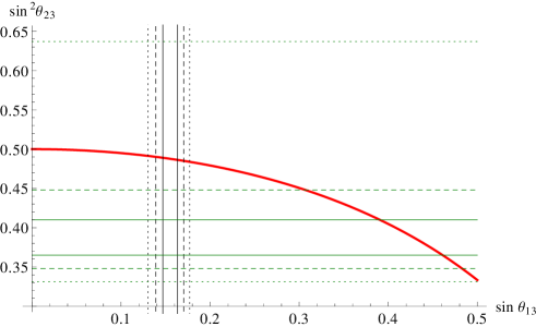
Figure 1: The thick red line corresponds to the relation in eq.(26). The black and green lines show the $1\sigma,2\sigma,3\sigma$ contours (solid, dashed and dotted lines, respectively) for $\sin\theta_{13}$ and $\sin^{2}\theta_{23}$, as obtained in [8] (see Table 1).

As for the neutrino angle $\theta^{\nu}_{12}$, we will consider two cases:

• bimaximal mixing (BM): $\theta^{\nu}_{12}=\displaystyle\frac{\pi}{4}$ (as also predicted by models with approximate conservation of $L^{\prime}=L_{e}-L_{\mu}-L_{\tau}$ );

• tri-bimaximal mixing (TBM): $\theta^{\nu}_{12}=\displaystyle\sin^{-1}\frac{1}{\sqrt{3}}$.

Since in the approach we are following the four parameters of the PMNS matrix (the three measured angles $\theta_{12}$, $\theta_{23}$, $\theta_{13}$ and the CPV Dirac phase $\delta$) will be expressed in terms of only three parameters (the two angles $\theta^{e}_{12}$, $\hat{\theta}_{23}$ and the phase $\phi$), the values of $\theta_{12}$, $\theta_{23}$, $\theta_{13}$ and $\delta$ will be correlated. More specifically, $\delta$ can be expressed as a function of the three angles, $\delta=\delta(\theta_{12},\theta_{23},\theta_{13})$, and its value will be determined by the values of the angles. As a consequence, the $J_{CP}$ factor also will be a function of $\theta_{12}$, $\theta_{23}$ and $\theta_{13}$, which will allow us to obtain predictions for the magnitude of the CP violation effects in neutrino oscillations using the current data on $\sin^{2}\theta_{12}$, $\sin^{2}\theta_{23}$ and $\sin\theta_{13}$.

We note first that using eq. (23) we can express $\sin^{2}\theta_{23}$ in terms of $\sin^{2}\hat{\theta}_{23}$ and $\sin^{2}\theta_{13}$:

$$\sin^{2}\theta_{23}=\frac{\sin^{2}\hat{\theta}_{23}-\sin^{2}\theta_{13}}{1-\sin^{2}\theta_{13}}\,,~{}~{}\cos^{2}\theta_{23}=\frac{\cos^{2}\hat{\theta}_{23}}{1-\sin^{2}\theta_{13}}\,.$$ (27)

It follows from these equations that $\hat{\theta}_{23}$ differs little from $\theta_{23}$ (it is somewhat larger). Further, using eqs. (23) and (27), we can express $\sin^{2}\theta_{12}$ in terms of $\theta^{\nu}_{12}$, $\theta_{23}$, $\theta_{13}$ and $\phi$:

$$\sin^{2}\theta_{12} =\left(1-\cos^{2}\theta_{23}\cos^{2}\theta_{13}\right)^{-1}\,\left[\sin^{2}\theta^{\nu}_{12}\sin^{2}\theta_{23}+\cos^{2}\theta^{\nu}_{12}\cos^{2}\theta_{23}\sin^{2}\theta_{13}\right.$$ (28)

$$+\left.\frac{1}{2}\,\sin 2\theta^{\nu}_{12}\sin 2\theta_{23}\sin\theta_{13}\cos\phi\right]\,.$$

As we have already indicated, we will use in the analysis which follows two specific values of $\theta^{\nu}_{12}=\pi/4$ (BM or LC); $\sin^{-1}(1/\sqrt{3})$ (TBM). Equation (28) will lead in each of the two cases to a new type of “sum rules”, i.e., to a correlation between the value of $\theta_{12}$ and the values of $\theta_{23}$, $\theta_{13}$ and $\phi$. In the case of bimaximal and tri-bimaximal $\theta^{\nu}_{12}$, the sum rules have the form:

$${\rm BM:}\quad \sin^{2}\theta_{12}=\frac{1}{2}\,+\frac{1}{2}\,\frac{\sin 2\theta_{23}\sin\theta_{13}\cos\phi}{1-\cos^{2}\theta_{23}\cos^{2}\theta_{13}}$$ (29)

$$\cong\frac{1}{2}+\cot\theta_{23}\sin\theta_{13}\cos\phi\left(1-\cot^{2}\theta_{23}\sin^{2}\theta_{13}+\mathcal{O}(\cot^{4}\theta_{23}\sin^{4}\theta_{13})\right)\,,$$ (30)

$${\rm TBM:}\quad \sin^{2}\theta_{12}=\frac{1}{3}\left(2+\frac{\sqrt{2}\,\sin 2\theta_{23}\sin\theta_{13}\cos\phi-\sin^{2}\theta_{23}}{1-\cos^{2}\theta_{23}\cos^{2}\theta_{13}}\right)$$ (31)

$$\cong\frac{1}{3}\,\left[1+2\sqrt{2}\,\cot\theta_{23}\sin\theta_{13}\cos\phi\,\left(1-\cot^{2}\theta_{23}\sin^{2}\theta_{13}\right)\right.$$

$$+\left.\cot^{2}\theta_{23}\sin^{2}\theta_{13}+\mathcal{O}(\cot^{4}\theta_{23}\sin^{4}\theta_{13})\right]\,.$$ (32)

The expressions for $\sin^{2}\theta_{12}$ in eqs. (29) and (31) are exact, while those given in eqs. (30) and (32) are obtained as expansions in the small parameter $\cot^{2}\theta_{23}\sin^{2}\theta_{13}$. The latter satisfies $\cot^{2}\theta_{23}\sin^{2}\theta_{13}\lesssim 0.063$ if $\sin^{2}\theta_{23}$ and $\sin^{2}\theta_{13}$ are varied in the $3\sigma$ intervals quoted in Table 1. To leading order in $\sin\theta_{13}$ the sum rule in eq. (30) was derived in [12].

We note next that since $\theta_{12}$, $\theta_{23}$ and $\theta_{13}$ are known, eq. (28) allows us to express $\cos\phi$ as a function of $\theta_{12}$, $\theta_{23}$ and $\theta_{13}$ and to obtain the range of possible values of $\phi$. Indeed, it follows from eqs. (29) and (31) that

$${\rm BM:}\qquad \cos\phi=-\,\frac{\cos 2\theta_{12}\,(1-\cos^{2}\theta_{23}\cos^{2}\theta_{13})}{\sin 2\theta_{23}\,\sin\theta_{13}}\,,$$ (33)

$${\rm TBM:}\qquad \cos\phi=\frac{(3\sin^{2}\theta_{12}-2)\,(1-\cos^{2}\theta_{23}\cos^{2}\theta_{13})+\sin^{2}\theta_{23}}{\sqrt{2}\sin 2\theta_{23}\,\sin\theta_{13}}\,.$$ (34)

Taking for simplicity for the best fit values of the three angles in the PMNS matrix $\sin^{2}\theta_{12}=0.31$, $\sin^{2}\theta_{23}=0.39$ and $\sin\theta_{13}=0.16$ (see Table 1), we get:

$$\cos\phi\cong-\,0.99\,~{}{\rm(BM)};\qquad\cos\phi\cong-\,0.20\,,~{}{\rm(TBM)}.$$ (35)

Equating the imaginary and real parts of $U_{e1}^{*}U_{\mu 3}^{*}U_{e3}U_{\mu 1}$ in the standard parametrisation and in the parametrisation under discussion one can obtain a relation between the CPV phases $\delta$ and $\phi$. We find for the BM case ($\theta^{\nu}_{12}=\pi/4$):

$$\sin\delta= \;-\,\frac{\sin\phi}{\sin 2\theta_{12}}\,,$$ (36)

$$\cos\delta= \;\frac{\cos\phi}{\sin 2\theta_{12}}\,\left(\frac{2\,\sin^{2}\theta_{23}}{\sin^{2}\theta_{23}\cos^{2}\theta_{13}+\sin^{2}\theta_{13}}-1\right)\,.$$ (37)

Since, as can be easily shown,

$$\sin 2\theta_{12}=\left(1-4\frac{\cot^{2}\theta_{23}\sin^{2}\theta_{13}\cos^{2}\phi}{(1+\cot^{2}\theta_{23}\sin^{2}\theta_{13})^{2}}\right)^{\frac{1}{2}}\,,$$ (38)

we indeed have to leading order in $\sin\theta_{13}$, $\sin\delta\cong-\sin\phi$ and $\cos\delta\cong\cos\phi$.

The expressions for $\sin\delta$ and $\cos\delta$ in eqs. (36) and (37) are exact. It is not difficult to check that we have $\sin^{2}\delta+\cos^{2}\delta=1$. Using the result for $\cos\phi$, eq. (33), we can get expressions for $\sin\delta$ and $\cos\delta$ in terms of $\theta_{12}$, $\theta_{23}$ and $\theta_{13}$. We give below the result for $\cos\delta$:

$$\cos\delta=-\,\frac{1}{2\sin\theta_{13}}\,\cot 2\theta_{12}\,\tan\theta_{23}\,\left(1-\cot^{2}\theta_{23}\,\sin^{2}\theta_{13}\right)\,.$$ (39)

Numerically we find for $\sin^{2}\theta_{12}=0.31$, $\sin^{2}\theta_{23}=0.39$ and $\sin\theta_{13}=0.16$:

$$\sin\delta\cong\pm 0.170\,,~{}~{}\cos\delta\cong-\,0.985\,.$$ (40)

Therefore, we have $\delta\simeq\pi$. For fixed $\sin^{2}\theta_{12}$ and $\sin\theta_{13}$, $|\cos\delta|$ increases with the increasing of $\sin^{2}\theta_{23}$. However, $\sin^{2}\theta_{23}$ cannot increase arbitrarily since eq. (29) and the measured values of $\sin^{2}\theta_{12}$ and $\sin^{2}\theta_{13}$ imply that the scheme with bimaximal mixing under discussion can be self-consistent only for values of $\sin^{2}\theta_{23}$, which do not exceed a certain maximal value. The latter is determined taking into account the uncertainties in the values of $\sin^{2}\theta_{12}$ and $\sin\theta_{13}$ in Section 3, where we perform a statistical analysis using the data on $\sin^{2}\theta_{23}$, $\sin^{2}\theta_{12}$, $\sin\theta_{13}$ and $\delta$ as given in [8].

In a similar way we obtain for the TBM case ($\theta^{\nu}_{12}=\sin^{-1}(1/\sqrt{3})$):

$$\sin\delta= \;-\,\frac{2\sqrt{2}}{3}\,\frac{\sin\phi}{\sin 2\theta_{12}}\,,$$ (41)

$$\cos\delta= \;\frac{2\sqrt{2}}{3\sin 2\theta_{12}}\,\cos\phi\,\left(-1+\frac{2\sin^{2}\theta_{23}}{\sin^{2}\theta_{23}\cos^{2}\theta_{13}+\sin^{2}\theta_{13}}\,\right)$$

$$\;+\frac{1}{3\sin 2\theta_{12}}\,\frac{\sin 2\theta_{23}\,\sin\theta_{13}}{\sin^{2}\theta_{23}\cos^{2}\theta_{13}+\sin^{2}\theta_{13}}\,.$$ (42)

The results for $\sin\delta$ and $\cos\delta$ we have derived are again exact and, as can be shown, satisfy $\sin^{2}\delta+\cos^{2}\delta=1$. Using the above expressions and the expression for $\sin^{2}\theta_{12}$ given in eq. (31) and neglecting the corrections due to $\sin\theta_{13}$, we obtain $\sin\delta\simeq-\,\sin\phi$ and $\cos\delta\simeq\cos\phi$. With the help of eq. (34) we can express $\sin\delta$ and $\cos\delta$ in terms of $\theta_{12}$, $\theta_{23}$ and $\theta_{13}$. The result for $\cos\delta$ reads:

$$\cos\delta=\frac{\tan\theta_{23}}{3\sin 2\theta_{12}\sin\theta_{13}}\,\left[1+\left(3\sin^{2}\theta_{12}-2\right)\,\left(1-\cot^{2}\theta_{23}\,\sin^{2}\theta_{13}\right)\right]\,.$$ (43)

For the best fit values of $\sin^{2}\theta_{12}=0.31$, $\sin^{2}\theta_{23}=0.39$ and $\sin\theta_{13}=0.16$, we find:

$$\sin\delta\cong\pm 0.999\,,~{}~{}\cos\delta\cong-\,0.0490\,.$$ (44)

Thus, in this case $\delta\simeq\pi/2$ or $3\pi/2$. For $\sin^{2}\theta_{23}=0.50$ and the same values of $\sin^{2}\theta_{12}$ and $\sin^{2}\theta_{13}$ we get $\cos\delta\cong-0.096$ and $\sin\delta\cong\pm 0.995$.

The fact that the value of the Dirac CPV phase $\delta$ is determined (up to an ambiguity of the sign of $\sin\delta$) by the values of the three mixing angles $\theta_{12}$, $\theta_{23}$ and $\theta_{13}$ of the PMNS matrix, eqs. (39) and (43), are the most striking predictions of the scheme considered with standard ordering and bimaximal and tri-bimaximal mixing in the neutrino sector. For the best fit values of $\theta_{12}$, $\theta_{23}$ and $\theta_{13}$ we get $\delta\cong\pi$ and $\delta\cong\pi/2$ or $3\pi/2$ in the cases of bimaximal and tri-bimaximal mixing, respectively. These results imply also that in the scheme with standard ordering under discussion, the $J_{CP}$ factor which determines the magnitude of CP violation in neutrino oscillations is also a function of the three angles $\theta_{12}$, $\theta_{23}$ and $\theta_{13}$ of the PMNS matrix:

$$J_{CP}=J_{CP}(\theta_{12},\theta_{23},\theta_{13},\delta(\theta_{12},\theta_{23},\theta_{13}))=J_{CP}(\theta_{12},\theta_{23},\theta_{13})\,.$$ (45)

This allows to obtain predictions for the range of possible values of $J_{CP}$ using the current data on $\sin^{2}\theta_{12}$, $\sin^{2}\theta_{23}$ and $\sin\theta_{13}$. We present these predictions in Section 3. The predictions we derive for $\delta$ and $J_{CP}$ will be tested in the experiments searching for CP violation in neutrino oscillations, which will provide information on the value of the Dirac phase $\delta$.

We would like to note that the sum rules we obtain in the BM (LC) and TBM cases, eqs. (39) and (43), differ from the sum rules derived in [23] using van Dyck and Klein type discrete symmetries ($S_{4}$, $A_{4}$, $A_{5}$, etc.), and in [24] on the basis of $SU(5)$ GUT and $S_{4}$, $A_{4}$ and $\Delta(96)$ symmetries. More specifically, for the values of $\sin^{2}\theta_{12}$, $\sin^{2}\theta_{23}$ and $\sin^{2}\theta_{13}$, compatible with current global neutrino oscillation data, for instance, the predictions for the value of the CPV phase $\delta$ obtained in the present study differ from those found in [23, 24]. The same comment is valid also for the possible ranges of values of $\sin^{2}\theta_{12}$ and $\sin^{2}\theta_{23}$ found by us and in [23]. Our predictions for $\delta$ agree with the ones reviewed in [24] in the context of charged lepton corrections, once we take the particular case $\hat{\theta}_{23}=\theta_{23}^{\nu}$.

2.2 Inverse Ordering

As anticipated, we also study for completeness the case where the diagonalisation of the charged lepton mass matrix gives rise to the inverse ordering in eq. (21). The PMNS matrix, in this case, can be written as [11]

$$U=R_{23}(\tilde{\theta}^{e}_{23})R_{12}(\tilde{\theta}^{e}_{12})\Psi R_{23}(\theta^{\nu}_{23})R_{12}(\theta^{\nu}_{12})\tilde{Q},$$ (46)

where unphysical phases have been eliminated, $\tilde{Q}$ contains the two Majorana phases, and $\Psi=\operatorname{diag}(1,e^{i\psi},e^{i\omega})$. Unlike in the case of standard ordering, it is not possible to combine the 23 rotation in the neutrino and charged lepton sector and describe them with a single parameter, $\hat{\theta}_{23}$. After fixing $\theta^{\nu}_{23}$ and $\theta^{\nu}_{12}$, we therefore have, in addition to the Majorana phases, four independent physical parameters, two angles and two phases, one more with respect to the case of standard ordering. In particular, it is not possible anymore to write the mixing matrix in terms of one physical Dirac CPV phase only. Thus, in this case the four parameters of the PMNS matrix (the three angles $\theta_{12}$, $\theta_{23}$ and $\theta_{13}$ and the Dirac CPV phase $\delta$) will be expressed in terms of the four parameters of the inverse ordering parametrisation of the PMNS matrix, eq. (46). We have for $\sin\theta_{13}$, $\sin\theta_{23}$ and $\sin\theta_{12}$:

$$\begin{split}\sin\theta_{13}=&\;\tilde{s}^{e}_{12}s^{\nu}_{23},\\ \sin\theta_{23}=&\;s^{\nu}_{23}\frac{\left|(t^{\nu}_{23})^{-1}\tilde{s}^{e}_{23}+e^{i(\psi-\omega)}\tilde{c}^{e}_{12}\tilde{c}^{e}_{23}\right|}{\sqrt{1-(\tilde{s}^{e}_{12}s^{\nu}_{23})^{2}}},\\ \sin\theta_{12}=&\;s^{\nu}_{12}\frac{\left|\tilde{c}^{e}_{12}+e^{i\psi}(t^{\nu}_{12})^{-1}\tilde{s}^{e}_{12}c^{\nu}_{23}\right|}{\sqrt{1-(\tilde{s}^{e}_{12}s^{\nu}_{23})^{2}}}.\end{split}$$ (47)

Given that the expressions for $\theta_{23}$ and $\theta_{13}$ do not depend on the value of $\theta_{12}^{\nu}$, they will be the same for bimaximal and tri-bimaximal mixing (in both cases $\theta^{\nu}_{23}=\frac{\pi}{4}$):

$$\sin\theta_{13} =\frac{\sin\tilde{\theta}^{e}_{12}}{\sqrt{2}},$$ (48)

$$\sin^{2}\theta_{23} =\frac{1}{2}\frac{1+\sin 2\tilde{\theta}_{23}^{e}\sqrt{\cos 2\theta_{13}}\cos\omega^{\prime}-2\sin^{2}\theta_{13}\cos^{2}\tilde{\theta}_{23}^{e}}{\cos^{2}\theta_{13}}$$ (49)

$$\cong\frac{1}{2}\left(1+\sin 2\tilde{\theta}_{23}^{e}\,\cos\omega^{\prime}-\,\cos 2\tilde{\theta}_{23}^{e}\,\sin^{2}\theta_{13}+\mathcal{O}(\sin^{4}\theta_{13})\,\right)\,,$$ (50)

where the phase $\omega^{\prime}=\psi-\omega$. The expression (50) for $\sin^{2}\theta_{23}$ is approximate, the corrections being of the order of $\sin^{4}\theta_{13}$ or smaller.

For each value of the phase $\psi$, any value of $\theta_{13}$ and $\theta_{23}$ in the experimentally allowed range at a given C.L., can be reproduced for an appropriate choice of $\omega^{\prime}$, $\theta_{12}^{e}$ and $\theta_{23}^{e}$. This is not always the case for the solar neutrino mixing angle $\theta_{12}$, as we will see in Section 4. Using eqs. (48), $\sin^{2}\theta_{12}$ can be expressed in terms of $\theta_{13}$ and $\psi$ as follows:

• bimaximal mixing (BM${}_{\text{IO}}$), $\theta^{\nu}_{12}=\displaystyle\frac{\pi}{4}$:

  $$\sin^{2}\theta_{12} =\frac{1}{2\cos^{2}\theta_{13}}\left(1+2\sin\theta_{13}\sqrt{\cos 2\theta_{13}}\cos\psi-\sin^{2}\theta_{13}\right)$$ (51)

  $$\simeq\frac{1}{2}+\sin\theta_{13}\,\cos\psi+\mathcal{O}(\sin^{5}\theta_{13})\,;$$ (52)

• tri-bimaximal mixing (TBM${}_{\text{IO}}$), $\theta^{\nu}_{12}=\sin^{-1}\frac{1}{\sqrt{3}}$:

  $$\sin^{2}\theta_{12} =\frac{1}{3\cos^{2}\theta_{13}}\left(1+2\sqrt{2}\sin\theta_{13}\sqrt{\cos 2\theta_{13}}\cos\psi\right)$$ (53)

  $$\simeq\frac{1}{3}\,(1+\sin^{2}\theta_{13})+\frac{2\sqrt{2}}{3}\sin\theta_{13}\cos\psi+\mathcal{O}(\sin^{4}\theta_{13})\,.$$ (54)

The expressions for $\sin^{2}\theta_{12}$ in eqs. (51) and (53) are exact, while those given in (52) and (54) are obtained as expansions in $\sin^{2}\theta_{13}$ in which the terms up to $\mathcal{O}(\sin^{4}\theta_{13})$ and $\mathcal{O}(\sin^{3}\theta_{13})$, respectively, were kept. Note that the corrections to the approximate expressions for $\sin^{2}\theta_{12}$ are negligibly small, being $\mathcal{O}(\sin^{4}\theta_{13})$. This together with eq. (52) and the $3\sigma$ ranges of allowed values of $\sin^{2}\theta_{12}$ and $\sin\theta_{13}$ quoted in Table 1 suggests that the bimaximal mixing scheme considered by us can be compatible with the current ($3\sigma$) data on $\sin^{2}\theta_{12}$ and $\sin\theta_{13}$ only for a very limited interval of negative values of $\cos\psi$ close to ($-1$).

It follows from eqs. (51) and (53) that the value of $\cos\psi$ is determined by the values of the PMNS angles $\theta_{12}$ and $\theta_{13}$. At the same time, $\sin^{2}\theta_{23}$ depends on two parameters: $\omega^{\prime}$ and $\theta_{23}^{e}$. This implies that the values of $\omega^{\prime}$ and $\theta_{23}^{e}$ are correlated, but cannot be fixed individually using the data on $\sin^{2}\theta_{23}$.

It is not difficult to derive also the expressions for the $J_{CP}$ factor in terms of the inverse ordering parameters in the two cases of values of $\theta^{\nu}_{12}$ of interest:

$$\!\!\!{\rm BM:}\;\;\;J_{CP}\simeq -\,\frac{\sin\theta_{13}}{4}\left(\sin\psi\cos 2\tilde{\theta}_{23}^{e}+\sin\omega^{\prime}\cos\psi\sin 2\tilde{\theta}_{23}^{e}\right)+\mathcal{O}(\sin^{2}\theta_{13})\,,$$ (55)

$$\!\!\!{\rm TBM:}\;\;\;J_{CP}\simeq -\,\frac{\sin\theta_{13}}{3\sqrt{2}}\left(\sin\psi\cos 2\tilde{\theta}_{23}^{e}+\sin\omega^{\prime}\cos\psi\sin 2\tilde{\theta}_{23}^{e}\right)+\mathcal{O}(\sin^{2}\theta_{13})\,.$$ (56)

We have not discussed here the LC case (conservation of the lepton charge $L^{\prime}=L_{e}-L_{\mu}-L_{\tau}$) as it involves five parameters ($\theta^{e}_{23}$, $\theta^{e}_{12}$, $\theta^{\nu}_{23}$, and two CPV phases). At the same time, the “minimal” LC case with $\theta^{e}_{23}=0$ is equivalent to the standard ordering case with BM mixing (i.e., with $\theta^{\nu}_{12}=\pi/4$) analised in detail in the previous subsection.

As in the case of the standard ordering, to obtain the CPV phase $\delta$ of the standard parametrisation of the PMNS matrix from the variables of these models, that is the function $\delta=\delta(\psi,\omega,\tilde{\theta}_{23}^{e},\theta_{13})$, we equate the imaginary and real parts of $U_{e1}^{*}U_{\mu 3}^{*}U_{e3}U_{\mu 1}$ in the two parametrisations.

3 Results with Standard Ordering

In the numerical analysis presented here, we use the data on the neutrino mixing parameters obtained in the global fit of [8] to constrain the mixing parameters of the setup described in Section 2. Our goal is first of all to derive the allowed ranges for the Dirac phase $\delta$, the $J_{CP}$ factor and the atmospheric neutrino mixing angle parameter $\sin^{2}\theta_{23}$. We will also obtain the allowed values of $\sin^{2}\theta_{12}$ and $\sin^{2}\theta_{13}$. We start in this Section by considering the standard ordering setup, and in particular the two different choices for the angle $\theta_{12}^{\nu}$: $\theta_{12}^{\nu}=\pi/4$ (BM and LC), $\theta_{12}^{\nu}=\sin^{-1}(1/\sqrt{3})$ (TBM).

Standard Ordering - Normal Hierarchy

Tribimaximal

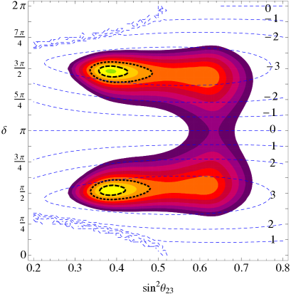
(a)

Bimaximal

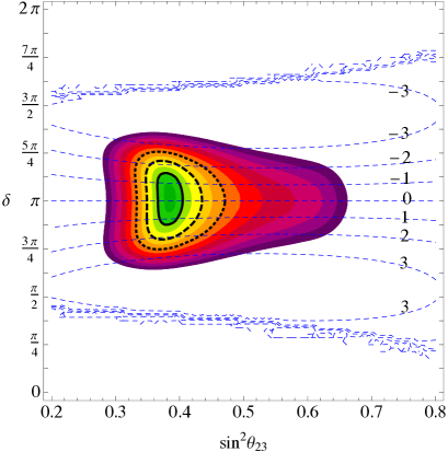
(b)

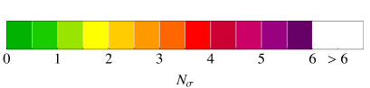
Figure 2: Contour plots for $N_{\sigma}=\sqrt{\chi^{2}}$ in the standard ordering setup and normal hierarchy of neutrino masses. The value of the reactor angle $\theta_{13}$ has been marginalized. The solid, dashed and dotted thick lines represent respectively the $1\sigma,2\sigma$ and $3\sigma$ contours. The dashed blue lines are contours of constant $\left|J_{CP}\right|$ in units of $10^{-2}$.

We construct the likelihood function and the $\chi^{2}$ for both schemes of bimaximal and tri-bimaximal mixing as described in Appendix B, using as parameters for this model $\sin\theta_{13}$, $\sin^{2}\theta_{23}$ and $\delta$, and exploiting the constraints on $\sin^{2}\theta_{12}$, $\sin^{2}\theta_{23}$, $\sin^{2}\theta_{13}$ and on $\delta$ obtained in [8].

Standard Ordering - Tribimaximal
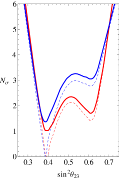
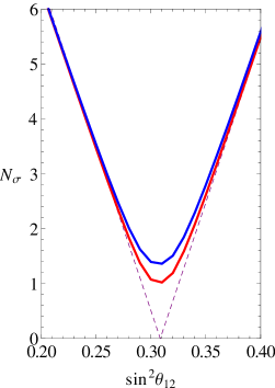
Standard Ordering - Bimaximal

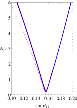
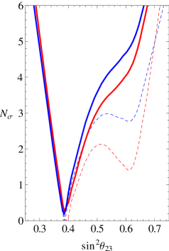
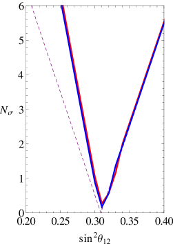
Figure 3: $N_{\sigma}$ as a function of each mixing angle for the TBM and BM models in the standard ordering setup. The dashed lines represent the results of the global fit reported in [8] while the thick ones represent the results we obtain in our setup. Blue lines are for normal hierarchy while the red ones are for inverted hierarchy (we used purple when the two bounds are approximately identical). These bounds are obtained minimizing the value of $N_{\sigma}$ in the parameter space for fixed value of the showed mixing angle.

Standard Ordering - Tribimaximal
         
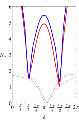
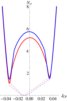
Standard Ordering - Bimaximal
         

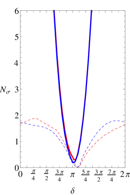
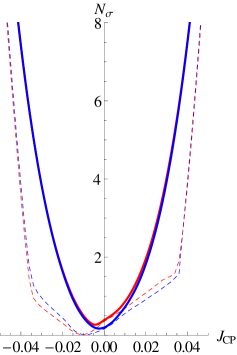
Figure 4: $N_{\sigma}$ as a function of $\delta$ and $J_{CP}$ for the TBM and BM models in the standard ordering setup. The dashed lines represent the results of the global fit reported in [8] while the thick ones represent the results we obtain in our setup. Blue lines are for normal hierarchy while the red ones are for inverted hierarchy. These bounds are obtained minimizing the value of $N_{\sigma}$ in the parameter space for a fixed value of $\delta$ (left plots) or $J_{CP}$ (right plots).

In Fig. 2 we show the contours of $N_{\sigma}=\sqrt{\chi^{2}}$ in the ($\sin^{2}\theta_{23},\delta$) plane, where the value of $\sin\theta_{13}$ has been marginalized. The blue dashed lines represent the contours of constant $J_{CP}$ (in units of $10^{-2}$). In Figs. 3 and 4, starting from the same likelihood function, we show the bounds on the neutrino mixing parameters and $J_{CP}$ in each scheme, both for normal and inverted neutrino mass hierarchy. These bounds are obtained minimizing the $\chi^{2}$ in the parameter space of the model, keeping as a constraint the value of the corresponding parameter. To make a direct comparison of the bounds obtained in the scheme considered by us with the general bounds obtained in the global fit in [8], we show the results from [8] with thin dashed lines. Thus, the thin dashed lines in Fig. 4 are the bounds on $J_{CP}$ obtained using directly the results of the global fit [8] and eq. (24), and represent the present status of our knowledge on this observable assuming the standard $3$-neutrino mixing setup . The thick solid lines represent the results obtained in the scheme with standard ordering considered. The blue and red color lines correspond respectively to the cases of normal and inverted neutrino mass hierarchy; in the case when the two bounds are essentially identical we used purple color lines.

From Figs. 2 and 3 we see that both the tribimaximal and bimaximal cases are well compatible with data. The $1\sigma$ difference between the minimum of $N_{\sigma}$ in the two cases is due to the fact that the bound on $\delta$ obtained in [8] favours values of $\delta\sim\pi$ (see Table 1), which is indeed the value needed in the bimaximal mixing (or LC) scheme to lower the value of $\theta_{12}$ from $\theta_{12}^{\nu}=\pi/4$, while the tri-bimaximal mixing scheme prefers $|\cos\delta|\ll 1$ (see Subsection 2.1).

The results we obtain for $\sin^{2}\theta_{12}$, $\sin^{2}\theta_{23}$ and $\sin^{2}\theta_{13}$ (i.e., the best fit values and the $3\sigma$ ranges) in the case of tri-bimaximal mixing are similar to those given in [8]. In contrast, our results for the Dirac phase $\delta$ and, correspondingly, for the $J_{CP}$ factor, are drastically different. For the best fit values and the $3\sigma$ allowed ranges of $\delta$ and $J_{CP}$ we find (see also Table 2):

		Best fit	3$\sigma$ range
	$J_{CP}$ (NH)	$-0.034$	$-0.039\div-0.028\oplus 0.028\div 0.039$
	$J_{CP}$ (IH)	$-0.034$	$-0.039\div-0.026\oplus 0.027\div 0.039$
	$\delta$ (NH)	$4.64$	$1.38\div 1.97\oplus 4.29\div 4.91$
TBM	$\delta$ (IH)	$4.64$	$1.39\div 2.17\oplus 4.04\div 4.93$
	$\sin\theta_{13}$	$0.16$	$0.13\div 0.18$
	$\sin^{2}\theta_{23}$ (NH)	$0.39$	$0.33\div 0.64$
	$\sin^{2}\theta_{23}$ (IH)	$0.39$	$0.34\div 0.66$
	$\sin^{2}\theta_{12}$	$0.31$	$0.25\div 0.36$
	$J_{CP}$	$0.00$	$-0.027\div 0.026$
	$\delta$ (NH)	$3.20$	$2.35\div 3.95$
	$\delta$ (IH)	$3.27$	$2.37\div 3.94$
BM	$\sin\theta_{13}$	$0.16$	$0.13\div 0.18$
	$\sin^{2}\theta_{23}$ (NH)	$0.38$	$0.33\div 0.47$
	$\sin^{2}\theta_{23}$ (IH)	$0.39$	$0.34\div 0.50$
	$\sin^{2}\theta_{12}$	$0.31$	$0.28\div 0.36$

Table 2: Best fit and 3$\sigma$ ranges (found fixing $\sqrt{\chi^{2}-\chi^{2}_{min}}=3$) in the standard ordering setup. When not explicitly indicated otherwise, the result applies both for normal hierarchy and inverted hierarchy of neutrino masses.

$${\rm NH:}\quad\delta\cong 4.64\cong\frac{3\pi}{2}\,, 1.38\mathrel{\hbox to0.0pt{\raise 2.20013pt\hbox{$<$}\hss}{\lower 2.20013pt\hbox{$\sim$}}}\delta\mathrel{\hbox to0.0pt{\raise 2.20013pt\hbox{$<$}\hss}{\lower 2.20013pt\hbox{$\sim$}}}1.97\,, {\rm or}$$ (57)

$$4.29\mathrel{\hbox to0.0pt{\raise 2.20013pt\hbox{$<$}\hss}{\lower 2.20013pt\hbox{$\sim$}}}\delta\mathrel{\hbox to0.0pt{\raise 2.20013pt\hbox{$<$}\hss}{\lower 2.20013pt\hbox{$\sim$}}}4.91\,,$$ (58)

$${\rm IH:}\quad\delta\cong 4.64\cong\frac{3\pi}{2}\,, 1.39\mathrel{\hbox to0.0pt{\raise 2.20013pt\hbox{$<$}\hss}{\lower 2.20013pt\hbox{$\sim$}}}\delta\mathrel{\hbox to0.0pt{\raise 2.20013pt\hbox{$<$}\hss}{\lower 2.20013pt\hbox{$\sim$}}}2.17\,, {\rm or}$$ (59)

$$4.04\mathrel{\hbox to0.0pt{\raise 2.20013pt\hbox{$<$}\hss}{\lower 2.20013pt\hbox{$\sim$}}}\delta\mathrel{\hbox to0.0pt{\raise 2.20013pt\hbox{$<$}\hss}{\lower 2.20013pt\hbox{$\sim$}}}4.93\,,$$ (60)

$${\rm NH:}\quad J_{CP}\cong-0.034\,, 0.028\mathrel{\hbox to0.0pt{\raise 2.20013pt\hbox{$<$}\hss}{\lower 2.20013pt\hbox{$\sim$}}}J_{CP}\mathrel{\hbox to0.0pt{\raise 2.20013pt\hbox{$<$}\hss}{\lower 2.20013pt\hbox{$\sim$}}}0.039\,, {\rm or}$$ (61)

$$-0.039\mathrel{\hbox to0.0pt{\raise 2.20013pt\hbox{$<$}\hss}{\lower 2.20013pt\hbox{$\sim$}}}J_{CP}\mathrel{\hbox to0.0pt{\raise 2.20013pt\hbox{$<$}\hss}{\lower 2.20013pt\hbox{$\sim$}}}-0.028\,,$$ (62)

$${\rm IH:}\quad J_{CP}\cong-0.034\,, 0.027\mathrel{\hbox to0.0pt{\raise 2.20013pt\hbox{$<$}\hss}{\lower 2.20013pt\hbox{$\sim$}}}J_{CP}\mathrel{\hbox to0.0pt{\raise 2.20013pt\hbox{$<$}\hss}{\lower 2.20013pt\hbox{$\sim$}}}0.039\,, {\rm or}$$ (63)

$$-0.039\mathrel{\hbox to0.0pt{\raise 2.20013pt\hbox{$<$}\hss}{\lower 2.20013pt\hbox{$\sim$}}}J_{CP}\mathrel{\hbox to0.0pt{\raise 2.20013pt\hbox{$<$}\hss}{\lower 2.20013pt\hbox{$\sim$}}}-0.026\,.$$ (64)

The $3\sigma$ intervals of allowed values of $\delta$ ($J_{CP}$) in eqs. (57) and (59) (eqs. (61) and (63)) are associated with the local minimum at $\delta\cong\pi/2$ ($J_{CP}\cong 0.034$) in Fig. 4 upper left (right) panel, while those given in eqs. (58) and (60) (eqs. (62) and (64)) are related to the absolute minimum at $\delta\cong 3\pi/2$ ($J_{CP}\cong-0.034$).

The results we have obtained, reported in Figs. 2 and 4, and in eqs. (57) - (64), are quasi-degenerate with respect to $J_{CP}\rightarrow-J_{CP}$, or $\delta\rightarrow(2\pi-\delta)$. This stems from the fact that the phase $\phi$ enters into the expressions for the mixing angles only via its cosine, see eqs. (29) and (31). This symmetry is slightly broken only by the explicit bound on $\delta$ given in [8], which is graphically represented in Fig. 4 by the asymmetry of the dashed lines showing that negative values of $J_{CP}$ are slightly favored.

As Figs. 2 and  4 show, in the case of tri-bimaximal mixing, the CP conserving values of $\delta=0;\pi;2\pi$ is excluded with respect to the best fit CP violating values $\delta\cong\pi/2;3\pi/2$ at more than $4\sigma$. Correspondingly, $J_{CP}=0$ is also excluded with respect to the best-fit values $J_{CP}\simeq(-0.034)$ and $J_{CP}\simeq 0.034$ at more than $4\sigma$. It follows from eqs. (57) - (64) (see also Table 2) that the $3\sigma$ allowed ranges of values of both $\delta$ and $J_{CP}$ form rather narrow intervals. These are the most striking predictions of the scheme with standard ordering and tri-bimaximal mixing under investigation.

We obtain different results assuming bimaximal mixing in the neutrino sector. Although in this case the best fit values of $\sin^{2}\theta_{12}$, $\sin^{2}\theta_{23}$, $\sin^{2}\theta_{13}$ and $\delta$ practically coincide with those found in [8], the $3\sigma$ allowed intervals of values of $\sin^{2}\theta_{12}$ and especially of $\sin^{2}\theta_{23}$ and $\delta$ differ significantly from those given in [8].

For the best fit values and the $3\sigma$ intervals of $\sin^{2}\theta_{12}$ and $\sin^{2}\theta_{23}$ we get (see also Table 2):

$$\sin^{2}\theta_{12}\cong 0.31\,,~{}~{}~{}0.28\mathrel{\hbox to0.0pt{\raise 2.20013pt\hbox{$<$}\hss}{\lower 2.20013pt\hbox{$\sim$}}}\sin^{2}\theta_{12}\mathrel{\hbox to0.0pt{\raise 2.20013pt\hbox{$<$}\hss}{\lower 2.20013pt\hbox{$\sim$}}}0.36\,;$$ (65)

$${\rm NH:}\quad\sin^{2}\theta_{23}\cong 0.38\,,~{}~{}0.33\mathrel{\hbox to0.0pt{\raise 2.20013pt\hbox{$<$}\hss}{\lower 2.20013pt\hbox{$\sim$}}}\sin^{2}\theta_{23}\mathrel{\hbox to0.0pt{\raise 2.20013pt\hbox{$<$}\hss}{\lower 2.20013pt\hbox{$\sim$}}}0.47\,;$$ (66)

$${\rm IH:}\quad\sin^{2}\theta_{23}\cong 0.39\,,~{}~{}0.34\mathrel{\hbox to0.0pt{\raise 2.20013pt\hbox{$<$}\hss}{\lower 2.20013pt\hbox{$\sim$}}}\sin^{2}\theta_{23}\mathrel{\hbox to0.0pt{\raise 2.20013pt\hbox{$<$}\hss}{\lower 2.20013pt\hbox{$\sim$}}}0.50\,.$$ (67)

As in [8], we find for the best fit value of $\delta$ and $J_{CP}$: $\delta\cong\pi$ and $J_{CP}\cong 0$. However, the $3\sigma$ range of $\delta$ and, correspondingly, of $J_{CP}$, we obtain differ from those derived in [8]:

$${\rm NH:}\quad 2.35\mathrel{\hbox to0.0pt{\raise 2.20013pt\hbox{$<$}\hss}{\lower 2.20013pt\hbox{$\sim$}}}\delta\mathrel{\hbox to0.0pt{\raise 2.20013pt\hbox{$<$}\hss}{\lower 2.20013pt\hbox{$\sim$}}}3.95\,;~{}~{}~{}~{}-\,0.027\mathrel{\hbox to0.0pt{\raise 2.20013pt\hbox{$<$}\hss}{\lower 2.20013pt\hbox{$\sim$}}}J_{CP}\mathrel{\hbox to0.0pt{\raise 2.20013pt\hbox{$<$}\hss}{\lower 2.20013pt\hbox{$\sim$}}}0.026\,.$$ (68)

$${\rm IH:}\quad 2.37\mathrel{\hbox to0.0pt{\raise 2.20013pt\hbox{$<$}\hss}{\lower 2.20013pt\hbox{$\sim$}}}\delta\mathrel{\hbox to0.0pt{\raise 2.20013pt\hbox{$<$}\hss}{\lower 2.20013pt\hbox{$\sim$}}}3.94\,;~{}~{}~{}~{}-\,0.027\mathrel{\hbox to0.0pt{\raise 2.20013pt\hbox{$<$}\hss}{\lower 2.20013pt\hbox{$\sim$}}}J_{CP}\mathrel{\hbox to0.0pt{\raise 2.20013pt\hbox{$<$}\hss}{\lower 2.20013pt\hbox{$\sim$}}}0.026\,.$$ (69)

We see, in particular, that also in this case the Dirac CPV phase $\delta$ is constrained to lie in a narrow interval around the value $\delta\simeq\pi$. This and the constraint $\sin^{2}\theta_{23}\lesssim 1/2$ are the most important predictions of the scheme with standard ordering and bimaximal neutrino mixing.

4 Results with the Inverse Ordering

The case of inverse ordering is qualitatively and quantitatively different from the case of standard ordering. For given values of $\theta_{12}^{\nu}$, $\theta^{\nu}_{23}$, the number of parameters is the same as in the PMNS matrix. Still, not all values of $U$ can be obtained, as we shall see.

The constraints on the reactor and atmospheric neutrino mixing angles are the same for bimaximal and tri-bimaximal mixing and can be derived directly from eq. (48). For any given value of the phase $\psi$, any values of $\theta_{13}$ and $\theta_{23}$ in the ranges

$$\begin{split}\qquad 0\leq\sin\theta_{13}\leq&\>\frac{1}{\sqrt{2}},\\ \qquad 0\leq\sin^{2}\theta_{23}\leq&\>\frac{\cos 2\theta_{13}}{\cos^{4}\theta_{13}}\simeq 1+\mathcal{O}(\sin^{2}\theta_{13}),\end{split}$$ (70)

can be obtained by an appropriate choice of $\omega^{\prime}$, $\theta^{e}_{12}$ and $\theta^{e}_{23}$. Clearly, the range of values allowed for $\theta_{13}$ and $\theta_{23}$ covers the full experimentally allowed range. The solar neutrino mixing angle can now be expressed in terms of $\theta_{13}$ and $\psi$ as in eq. (48). Any value of $\theta_{12}$ in the interval

$$\text{BM}_{IO}:$$

$$\frac{1}{2}\frac{1-2\sin\theta_{13}\sqrt{\cos 2\theta_{13}}-\sin^{2}\theta_{13}}{\cos^{2}\theta_{13}}\leq\sin^{2}\theta_{12} \leq\frac{1}{2}\frac{1+2\sin\theta_{13}\sqrt{\cos 2\theta_{13}}-\sin^{2}\theta_{13}}{\cos^{2}\theta_{13}},$$ (71)

$$\text{TBM}_{IO}:$$

$$\frac{1}{3}\frac{1-2\sqrt{2}\sin\theta_{13}\sqrt{\cos 2\theta_{13}}}{\cos^{2}\theta_{13}}\leq\sin^{2}\theta_{12} \leq\frac{1}{3}\frac{1+2\sqrt{2}\sin\theta_{13}\sqrt{\cos 2\theta_{13}}}{\cos^{2}\theta_{13}},$$ (72)

can then be obtained for an appropriate choice of $\psi$. At leading order in $\sin\theta_{13}$ these bounds become

$$\begin{split}\text{BM}_{IO}:&\quad\frac{1}{2}-\sin\theta_{13}\lesssim\sin^{2}\theta_{12}\lesssim\frac{1}{2}+\sin\theta_{13},\\ \text{TBM}_{IO}:&\quad\frac{1}{3}-\frac{2\sqrt{2}}{3}\sin\theta_{13}\lesssim\sin^{2}\theta_{12}\lesssim\frac{1}{3}+\frac{2\sqrt{2}}{3}\sin\theta_{13}.\end{split}$$ (73)

Given the experimental bounds on the PMNS angles found in the global fit [8], see Table 1, one can immediately notice that while the tri-bimaximal case is perfectly compatible with the data, the bimaximal case has a $\sim 2\sigma$ tension in the prediction of the solar neutrino mixing angle parameter $\sin^{2}\theta_{12}$.

Inverse Ordering - Tribimaximal

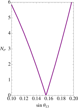
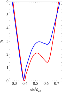
Inverse Ordering - Bimaximal

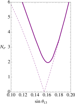
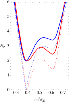
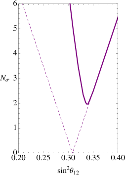
Figure 5: $N_{\sigma}$ as a function of each mixing angle for the TBM and BM models with the inverse ordering setup. The dashed lines represent the results of the global fit reported in [8] while the thick ones represent the results we obtain in our setup. Blue lines are for normal hierarchy while the red ones are for inverted hierarchy (we use purple when the two bounds are approximately identical). These bounds are obtained minimizing the value of $N_{\sigma}$ in the parameter space for fixed value of the showed mixing angle.

Inverse Ordering

Tribimaximal

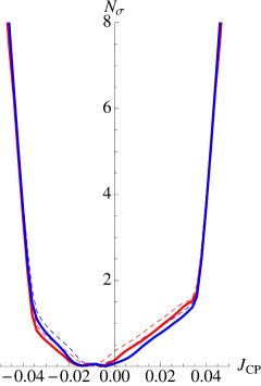
(a)

Bimaximal

(b)

Figure 6: $N_{\sigma}$ as a function of $J_{CP}$ for the TBM and BM models in the inverse ordering setup. The dashed lines represent the results of the global fit reported in [8] while the thick ones represent the results we obtain in our setup. Blue lines are for normal neutrino mass hierarchy while the red ones are for inverted hierarchy. These bounds are obtained minimizing the value of $N_{\sigma}$ in the parameter space for a fixed value of $J_{CP}$.

As was done for the standard ordering case, we construct the likelihood function and the $\chi^{2}$ for both models as described in Appendix B, exploiting the constraints on $\sin^{2}\theta_{12}$, $\sin^{2}\theta_{23}$, $\sin^{2}\theta_{13}$ and on $\delta$ obtained in [8], and using in this case as parameters $\sin\theta_{13}$, $\sin\theta_{23}^{e}$ and the phases $\psi$ and $\omega$. We show in Figs. 5 and 6 the bounds on the neutrino mixing angles and the $J_{CP}$ factor both in the cases of bimaximal and tri-bimaximal mixing in the neutrino sector, and for normal and inverted neutrino mass hierarchy.

From Fig. 5, we see that in the case of tribimaximal mixing (upper row), the intervals of allowed values of the PMNS mixing angles obtained in the model under discussion and in the global fit performed in [8] coincide. This is a consequence of the fact that the 4D parameter space of the model considered completely overlaps with the experimentally allowed parameter space in the PMNS parametrisation and therefore it does not give any additional constraint. It is consistent with the analytic bounds reported above as well.

In the case of bimaximal mixing instead (Fig. 5 lower row), only a portion of the relevant PMNS parameter space is reachable, a fact that is reflected in the bounds on $\sin^{2}\theta_{12}$ given in eq. (73). Values of $\theta_{12}$ in the upper part of its present experimental range are favoured in this case.

In both cases of tri-bimaximal and bimaximal mixing from the neutrino sector, the bounds on $\sin^{2}\theta_{13}$ and $\sin^{2}\theta_{12}$ corresponding to the normal and inverted neutrino mass hierarchy are approximately identical, while they differ for the atmospheric neutrino mixing angle and for the $J_{CP}$ factor.

Considering the expressions for $J_{CP}$ in eqs. (55) and (56) and Fig. 6, we see that within $\sim 1\sigma$ from the best-fit point, every value in the ranges

$$\left|J_{CP}^{BM}\right|\lesssim\frac{\sin\theta_{13}^{+1\sigma}}{4}\sim 0.04,\qquad\left|J_{CP}^{TBM}\right|\lesssim\frac{\sin\theta_{13}^{+1\sigma}}{3\sqrt{2}}\sim 0.038,$$ (74)

is allowed, where we have used the $1\sigma$ upper bound on $\sin\theta_{13}$ from Table 1. As a consequence, we cannot make more specific predictions about the CP violation due to the Dirac phases $\delta$ in this case. This is an important difference with respect to the standard ordering scheme where, in the tri-bimaximal mixing case, relatively large values of the $|J_{CP}|$ factor lying in a narrow interval are predicted at $3\sigma$ and, in the bimaximal mixing case, $\delta$ is predicted to lie at $3\sigma$ in a narrow interval around the value of $\delta\sim\pi$.

5 Summary and Conclusions

In this paper we considered the possibility that the neutrino mixing angle $\theta_{13}$ arises from the interplay of 12 and 23 rotations in the neutrino ($U_{\nu}$) and charged lepton ($U_{e}$) contributions to the PMNS neutrino mixing matrix ($U=U^{\dagger}_{e}U_{\nu}$). We generalized previous work [15] in two directions. First, we considered two possible orderings of 12 and 23 rotations in $U_{e}$, the “standard”, $U_{e}\sim R^{e}_{23}R^{e}_{12}$, and the “inverse”, $U_{e}\sim R^{e}_{12}R^{e}_{23}$, while keeping the standard ordering in the neutrino sector, $U_{\nu}\sim R^{\nu}_{23}R^{\nu}_{12}$. Second, in order to be able to accommodate a possible deviation of the atmospheric neutrino mixing angle $\theta_{23}$ from $\pi/4$, we allowed the charged lepton 23 rotation angle (and possibly the neutrino one, in the standard case) to assume arbitrary values. We considered the cases in which $U_{\nu}$ is in the bimaximal or tri-bimaximal form, or in the form resulting from the conservation of the lepton charge $L_{e}-L_{\mu}-L_{\tau}$ (LC). We took, of course, all relevant physical CP violation (CPV) phases into account.

The case of normal ordering turns out to be particularly interesting. The PMNS matrix can be parameterized in terms of the charged lepton and neutrino 12 rotation angles, $\theta^{e}_{12}$ and $\theta^{\nu}_{12}$, an effective 23 rotation angle, $\hat{\theta}_{23}\approx\theta_{23}$, and a CPV phase $\phi$. Once $\theta^{\nu}_{12}$ is fixed to the bimaximal (LC) or tri-bimaximal value, the number of parameters reduces to three, and the Dirac phase $\delta$ in the PMNS matrix can be predicted in terms of the PMNS solar, atmospheric and reactor neutrino mixing angles $\theta_{12}$, $\theta_{23}$ and $\theta_{13}$. Moreover, the range of possible values of the PMNS angles turns out to be constrained.

In the tri-bimaximal case, the Dirac CPV phase $\delta$ is predicted to have a value $\delta\approx\pi/2$ or $\delta\approx 3\pi/2$, implying nearly maximal CP violation in neutrino oscillations, while in the bimaximal (and LC) case we find $\delta\approx\pi$ and, consequently, the CP violation effects in neutrino oscillations are predicted to be small. The present data have a mild preference for the latter option (see Table 1 and, e.g., Fig. 4). Moreover, $\theta_{23}$ is predicted to be below $\pi/4$ in the bimaximal case, which is also in agreement with the indications from the current global neutrino oscillations data. In the set-up considered by us, the $\theta_{23}>\pi/4$ solution of the global fit analysis in [8] is disfavored.

The case of inverse ordering is qualitatively and quantitatively very different. Fixing $U_{\nu}$ to the bimaximal or tri-bimaximal form is not sufficient to obtain a prediction: the number of free physical parameters in this case is four – two angles and two CPV phases. Still, not all values of the four physical parameters in the PMNS matrix, $\theta_{12}$, $\theta_{23}$, $\theta_{13}$ and $\delta$, can be reached in this parameterization. In the tri-bimaximal case, the ranges of parameters that can be reached overlaps with the experimental ranges, so that no predictions can be made. In the bimaximal case, however, this is not the case. One obtains, in fact, the approximate relation $\sin^{2}\theta_{12}\gtrsim 1/2-\sin\theta_{13}$, which is barely compatible with the data. As a consequence, i) there is a tension in the above relation that worsen the quality of the fit, and ii) values of $\theta_{12}$ in the upper part of its present experimental range are preferred. In both cases, no predictions for the Dirac CPV phase $\delta$ can be made. We did not consider here the LC case as it involves, in general, five parameters, while its “minimal” version, corresponding to setting $\theta^{e}_{23}=0$, is equivalent to the standard ordering case with BM mixing (i.e., with $\theta^{\nu}_{12}=\pi/4$).

The fact that the value of the Dirac CPV phase $\delta$ is determined (up to an ambiguity of the sign of $\sin\delta$) by the values of the three PMNS mixing angles, $\theta_{12}$, $\theta_{23}$ and $\theta_{13}$, eqs. (39) and (43), are the most striking predictions of the scheme considered with standard ordering and bimaximal (LC) and tri-bimaximal mixing in the neutrino sector. As we have already indicated, for the best fit values of $\theta_{12}$, $\theta_{23}$ and $\theta_{13}$ we get $\delta\cong\pi$ and $\delta\cong\pi/2$ or $3\pi/2$ in the cases of bimaximal and tri-bimaximal mixing, respectively. These results imply also that in the scheme with standard ordering we have discussed, the $J_{CP}$ factor which determines the magnitude of CP violation in neutrino oscillations, is also a function of the three mixing angles: $J_{CP}=J_{CP}(\theta_{12},\theta_{23},\theta_{13},\delta(\theta_{12},\theta_{23},\theta_{13}))=J_{CP}(\theta_{12},\theta_{23},\theta_{13})$. This allowed us to obtain predictions for the range of possible values of $J_{CP}$ using the current data on $\sin^{2}\theta_{12}$, $\sin^{2}\theta_{23}$ and $\sin\theta_{13}$, which are given in eqs. (57) - (63) and eqs. (68) - (69).

The predictions for $\sin^{2}\theta_{23}$, and for $\delta$ and $J_{CP}$ we have obtained in the scheme with standard ordering and bimaximal (or LC) or tri-bimaximal form of $U_{\nu}$ will be tested by the neutrino oscillation experiments able to determine whether $\sin^{2}\theta_{23}\lesssim 0.5$ or $\sin^{2}\theta_{23}>0.5$, and in the experiments searching for CP violation in neutrino oscillations.

Aknowledgements

This work was supported in part by the INFN program on “Astroparticle Physics”, the Italian MIUR program on “Neutrinos, Dark Matter and Dark Energy in the Era of LHC” the World Premier International Research Center Initiative (WPI Initiative), MEXT, Japan (S.T.P.), by the European Union FP7-ITN INVISIBLES and UNILHC (Marie Curie Action, PITAN-GA-2011-289442 and PITN-GA-2009-23792), and by the ERC Advanced Grant no. 267985 “DaMESyFla”. Part of the work was done at the Galileo Galilei Institute for Theoretical Physics, Florence, Italy, which we thank for the kind hospitality and support.

Appendix

Appendix A Parametrisation of the PMNS matrix

In the present Appendix we show how the parametrisation of eq. (22) follows from the ones in eqs. (19) and (20). We start by writing explicitly the PMNS matrix as

$$U=\Phi^{*}_{e}R_{12}(\theta^{e}_{12})R_{23}(\theta_{23}^{e})\Psi R_{23}(\theta_{23}^{\nu})R_{12}(\theta_{12}^{\nu})\Phi_{\nu},$$ (75)

where $\Psi=\operatorname{diag}(1,e^{i\psi},e^{i\omega})$, without loss of generality. Any $2\times 2$ unitary matrix $V$ can be recast in the form $V=PR(\theta)Q$, where $P=\operatorname{diag}(e^{i\phi_{1}},e^{i\phi_{2}})$, $Q=\operatorname{diag}(1,e^{i\omega_{2}})$ and $R(\theta)$ is a $2\times 2$ rotation. We use this to write

$$R_{23}(\theta_{23}^{e})\Psi R_{23}(\theta_{23}^{\nu})=\Phi^{\prime}R_{23}(\hat{\theta}_{23})\Omega,$$ (76)

where $R_{23}(\hat{\theta}_{23})$ is an orthogonal rotation in the 23 block with

$$\sin\hat{\theta}_{23}=\left|\cos\theta_{23}^{e}\sin\theta_{23}^{\nu}+e^{i(\omega-\psi)}\sin\theta_{23}^{e}\cos\theta_{23}^{\nu}\right|,$$ (77)

$\Phi^{\prime}=\operatorname{diag}(e^{i\phi_{1}},e^{i\phi_{2}},e^{i\phi_{3}})$, and $\Omega=\operatorname{diag}(1,e^{i\omega_{2}},e^{i\omega_{3}})$. An explicit solution for the angles in terms of the original parameters is

$$\begin{split}&\phi_{1}=0,\qquad\phi_{2}=\delta_{c}+\delta_{s}+\psi-\omega,\qquad\phi_{3}=0,\\ &\omega_{2}=-\delta_{s}+\omega,\qquad\omega_{3}=-\delta_{c}+\omega,\end{split}$$ (78)

where

$$\begin{split}\delta_{s}&=\text{Arg}\left(\cos\theta_{23}^{e}\sin\theta_{23}^{\nu}+e^{i(\omega-\psi)}\sin\theta_{23}^{e}\cos\theta_{23}^{\nu}\right),\\ \delta_{c}&=\text{Arg}\left(\cos\theta_{23}^{e}\cos\theta_{23}^{\nu}-e^{i(\omega-\psi)}\sin\theta_{23}^{e}\sin\theta_{23}^{\nu}\right).\end{split}$$ (79)

Considering now also the $R_{12}(\theta_{12}^{\nu})$ rotation, we obtain

$$R_{23}(\hat{\theta}_{23})\Omega R_{12}(\theta_{12}^{\nu})=\Phi^{\prime\prime}R_{23}(\hat{\theta}_{23})R_{12}(\theta_{12}^{\nu})\>Q^{\prime\prime},$$ (80)

with $\Phi^{\prime\prime}=\operatorname{diag}(1,e^{i\omega_{2}},e^{i\omega_{2}})$ and $Q^{\prime\prime}=\operatorname{diag}(1,1,e^{i(\omega_{3}-\omega_{2})})$. The phases in $Q^{\prime\prime}$ add to the ones in $Q^{\prime}$ and are Majorana phases. The ones in $\Phi^{\prime\prime}$, instead, add to the ones in $\Phi^{\prime}$:

$$\Phi^{\prime}\Phi^{\prime\prime}=e^{i\phi_{1}}\operatorname{diag}(1,e^{i(\phi_{2}-\phi_{1}+\omega_{2})},e^{i(\phi_{3}-\phi_{1}+\omega_{2})}).$$ (81)

The phase in the 33 position commutes with $R_{12}(\theta_{12}^{e})$. Together with the overall phase $\phi_{1}$, it will describe the unphysical phase matrix $P$ in eq. (22):

$$P=e^{i\phi_{1}}\operatorname{diag}(1,1,e^{i(\phi_{3}-\phi_{1}+\omega_{2})}).$$ (82)

We see that the only physical Dirac CP violating phase in this parametrisation is contained in the matrix $\Phi=\operatorname{diag}(1,e^{i\phi},1)$, with

$$\phi=\phi_{2}-\phi_{1}+\omega_{2}=\psi+\delta_{c}.$$ (83)

Appendix B Statistical analysis

In this appendix we describe the simplified statistical analysis performed to obtain the results. Our aim is to use the results of the global fit performed in [8] to assess how well each of the models introduced in the previous section can fit the data. In particular, we use the constraints on the PMNS angles $\theta_{13},\theta_{12},\theta_{23}$ and on the phase $\delta$ for the normal hierarchy (NH) and inverted hierarchy (IH) cases, as derived in [8]. There, the results are reported by plotting the value of $N_{\sigma}\equiv\sqrt{\Delta\chi^{2}}$ (with $\Delta\chi^{2}=\chi^{2}-\chi^{2}_{min}$) as a function of each observable, with the remaining ones marginalized away. We construct an approximate global likelihood from these functions as

$$L_{j}(\alpha_{j})=\exp\left(-\frac{\Delta\chi_{j}^{2}(\alpha_{j})}{2}\right),\qquad L(\vec{\alpha})=\prod_{j}^{n}L_{j}(\alpha_{j}),$$ (84)

where $\vec{\alpha}=\{\sin^{2}\theta_{13},\sin^{2}\theta_{23},\sin^{2}\theta_{12},\delta\}$ are the observables relevant for our analysis, and we define

$$\chi^{2}(\vec{\alpha})\equiv-2\log L(\vec{\alpha})$$ (85)

and $N_{\sigma}(\vec{\alpha})=\sqrt{\chi^{2}(\vec{\alpha})}$. In using this procedure we loose any information about possible correlations between different observables. The effect of this loss of information is however negligible, as one can check comparing our 1$\sigma$, 2$\sigma$ and 3$\sigma$ contours in the $(\sin^{2}\theta_{23},\sin^{2}\theta_{13})$ and $(\sin^{2}\theta_{13},\delta)$ planes shown in Figure 7 with the ones in Fig. 1 and Fig. 2 of [8].

Figure 7: $1\sigma,2\sigma,3\sigma$ contours (respectively solid, dashed and dotted lines) of our global likelihood function in the $(\sin^{2}\theta_{23},\sin^{2}\theta_{13})$ plane (left) and $(\sin^{2}\theta_{13},\delta)$ plane (right), using the data for NH. These plots can be compared with Fig.1 and Fig.2 of [8] for NH. Undisplayed variables have been marginalized.

Each model introduced in the previous section (which we dub with an index $m$) depends on a set of parameters ${\bf x}^{m}=\{x^{m}_{i}\}$, which are related to the observables via expressions $\alpha_{j}=\alpha_{j}^{m}({\bf x}^{m})$, obtained from eqs. (23), (47). We then construct the likelihood function in the space of the parameters ${\bf x}^{m}$ as

$$L^{m}({\bf x}^{m})=L(\vec{\alpha}^{m}({\bf x}^{m})).$$ (86)

We define $\chi^{2}({\bf x}^{m})=-2\log L^{m}({\bf x}^{m})$ and $N_{\sigma}({\bf x}^{m})=\sqrt{\chi^{2}({\bf x}^{m})}$. The last one is the function we use to produce the plots shown in Figures 2-6. Finally, to obtain the best-fit point we use the maximum likelihood method.

Addendum: Analysis with the 2013 Data

We update our analysis using the results of the global fit performed in [1], in which the latest 2013 data from the Daya Bay, RENO, T2K and MINOS experiments are included. A global fit including the indicated 2013 data was performed also in [2] in which the authors report similar results. We restrict this update to the standard ordering case since the main conclusions for the inverse ordering one remain unchanged. In this new global fit the authors find, for the Dirac CP violating phase, the best fit value of $\delta\cong 3\pi/2$. The CP conserving values $0$ and $\pi$ are disfavored, respectively, at $1.7\sigma$ and $1.5\sigma$ ($2\sigma$ and $1\sigma$) in the case of NH (IH) neutrino mass spectrum, see Fig. 3 of [1]. Another relevant difference of the results of this fit with respect to the previously obtained one in [8] is that the hint for atmospheric angle in the first octant is now somewhat weaker than before: the best-fit value, located in the first octant, moved from $\sin^{2}\theta_{23}\simeq 0.39$ to $\sin^{2}\theta_{23}\simeq 0.43$, and the $\sqrt{\Delta\chi^{2}}$ of the relative minimum in the second octant dicreased from $\sim 3\sigma$ ($\sim 1.5\sigma$) to $\sim 2.2\sigma$ ($\sim 0.5\sigma$) for NH (IH) spectrum.

Using the new results from [1] we find that the CP conserving values of $\delta=0,\pi$ ($J_{CP}=0$) are excluded in the tri-bimaximal mixing (TBM) case at the level of $5\sigma$ both for the NH and IH spectra, as Figs. 8 and 10 show. The second minimum at $\delta\sim\pi/2$ is disfavored with respect to the best-fit point at the $\sim 2.6\sigma$ ($2.2\sigma$) level in the NH (IH) case. The allowed $3\sigma$ ranges are reported in Table 3. In what concerns the atmospheric neutrino mixing angle, Fig. 9 shows that, for TBM arising from the neutrino sector, the allowed range of $\sin^{2}\theta_{23}$ in the model considered follows closely the results of the global fit in [1]: in the NH case we find a mild ($\sim 2\sigma$) preference for the first octant, while in the IH case the two octants are approximately degenerate.

We have found earlier that the value of $\delta$ predicted in the bimaximal mixing (BM) case using the best fit values of the neutrino mixing angles, is $\delta\sim\pi$. As a consequence, the BM case is now mildly disfavored with respect to the TBM one:

$$\sqrt{\chi^{2}_{min,BM}-\chi^{2}_{min,TBM}}\simeq 1.5\;(1.2)\,,~{}~{}~{}{\rm NH~{}(IH)}\,.$$ (87)

This is due to the new bound on $\delta$ obtained in [1], see Fig. 10. For the atmospheric neutrino mixing angle $\theta_{23}$ we find in this case a preference for the first octant at the $\sim 3\sigma$ level, see Table 3 and Figs. 8, 9 .

Standard Ordering - Normal Hierarchy

Tribimaximal

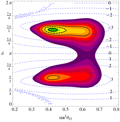
(a)

Bimaximal

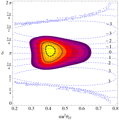
(b)

Figure 8: Contour plots for $N_{\sigma}=\sqrt{\chi^{2}}$ in the standard ordering setup and normal hierarchy of neutrino masses. The value of the reactor angle $\theta_{13}$ has been marginalized. The solid, dashed and dotted thick lines represent respectively the $1\sigma,2\sigma$ and $3\sigma$ contours. The dashed blue lines are contours of constant $\left|J_{CP}\right|$ in units of $10^{-2}$.

Standard Ordering - Tribimaximal
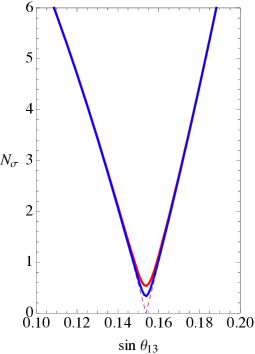
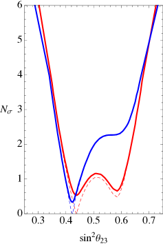
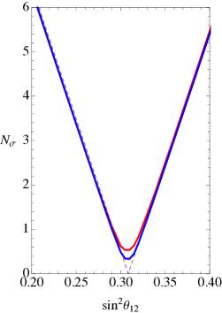
Standard Ordering - Bimaximal

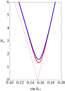
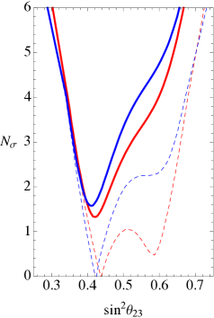
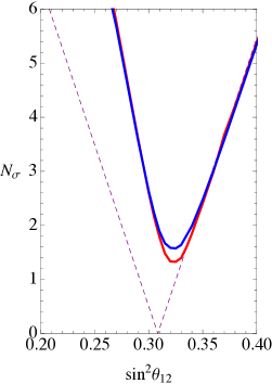
Figure 9: $N_{\sigma}$ as a function of each mixing angle for the TBM and BM models in the standard ordering setup. The dashed lines represent the results of the global fit reported in [1] while the thick ones represent the results we obtain in our setup. Blue lines are for normal hierarchy while the red ones are for inverted hierarchy (we used purple when the two bounds are approximately identical). These bounds are obtained minimizing the value of $N_{\sigma}$ in the parameter space for fixed value of the showed mixing angle.

Standard Ordering - Tribimaximal
         
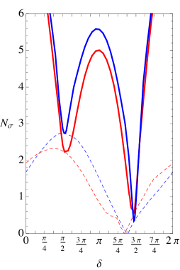
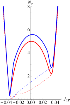
Standard Ordering - Bimaximal
         

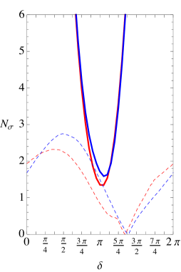
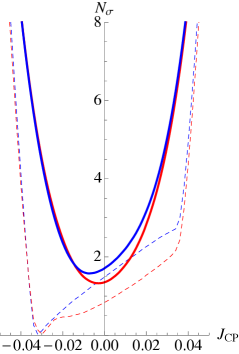
Figure 10: $N_{\sigma}$ as a function of $\delta$ and $J_{CP}$ for the TBM and BM models in the standard ordering setup. The dashed lines represent the results of the global fit reported in [1] while the thick ones represent the results we obtain in our setup. Blue lines are for normal hierarchy while the red ones are for inverted hierarchy. These bounds are obtained minimizing the value of $N_{\sigma}$ in the parameter space for a fixed value of $\delta$ (left plots) or $J_{CP}$ (right plots).

		Best fit	3$\sigma$ range
	$J_{CP}$ (NH)	$-0.034$	$-0.038\div-0.028\oplus 0.032\div 0.036$
	$J_{CP}$ (IH)	$-0.034$	$-0.039\div-0.024\oplus 0.027\div 0.037$
	$\delta$ (NH)	$4.63$	$1.53\div 1.80\oplus 4.24\div 4.92$
TBM	$\delta$ (IH)	$4.62$	$1.45\div 2.10\oplus 4.03\div 4.94$
	$\sin\theta_{13}$	$0.15$	$0.13\div 0.17$
	$\sin^{2}\theta_{23}$ (NH)	$0.43$	$0.36\div 0.64$
	$\sin^{2}\theta_{23}$ (IH)	$0.44$	$0.36\div 0.66$
	$\sin^{2}\theta_{12}$	$0.31$	$0.26\div 0.36$
	$J_{CP}(NH)$	$-0.008$	$-0.026\div 0.022$
	$J_{CP}(IH)$	$-0.003$	$-0.025\div 0.023$
	$\delta$ (NH)	$3.35$	$2.50\div 3.92$
BM	$\delta$ (IH)	$3.22$	$2.47\div 3.88$
	$\sin\theta_{13}$	$0.16$	$0.14\div 0.17$
	$\sin^{2}\theta_{23}$ (NH)	$0.41$	$0.35\div 0.50$
	$\sin^{2}\theta_{23}$ (IH)	$0.42$	$0.36\div 0.55$
	$\sin^{2}\theta_{12}$	$0.32$	$0.29\div 0.36$

Table 3: Best fit and 3$\sigma$ ranges (found fixing $\sqrt{\chi^{2}-\chi^{2}_{min}}=3$) in the standard ordering setup using the data from [1]. When not explicitly indicated otherwise, the result applies both for normal hierarchy and inverted hierarchy of neutrino masses.

References

- [1] K. Nakamura and S.T. Petcov, “Neutrino Mass, Mixing, and Oscillations”, in J. Beringer et al. (Particle Data Group), Phys. Rev. D86 (2012) 010001.
- [2] S.M. Bilenky, J. Hosek and S.T. Petcov, Phys. Lett. B94 (1980) 495.
- [3] E. Molinaro and S.T. Petcov, Eur. Phys. J. C61 (2009) 93 [arXiv:0803.4120].
- [4] L. Wolfenstein, Phys. Lett. B107 (1981) 77; S.M. Bilenky, N.P. Nedelcheva and S.T. Petcov, Nucl. Phys. B247 (1984) 61; B. Kayser, Phys. Rev. D30 (1984) 1023.
- [5] The most recent data on the neutrino masses, mixing and neutrino oscillations were reviewed recently in several presentations at Neutrino 2012, the XXV International Conference on Neutrino Physics and Astrophysics (June 4-10, 2012, Kyoto, Japan), available at the web-site neu2012.kek.jp.
- [6] F. P. An et al. [Daya-Bay Collaboration], Phys. Rev. Lett. 108 (2012) 17803 [arXiv:1203.1669]; F. P. An et al. [Daya-Bay Collaboration] [arXiv:1210.6327].
- [7] J.K. Ahn et al. [RENO Collaboration], [arXiv:1204.0626], Phys. Rev. Lett. 108 (2012) 191802; Y. Abe et al. [Double Chooz Collaboration] [arXiv:1207.6632]; T. Nakaya [for the T2K Collaboration], talk at Neutrino 2012 [5]; see also: K. Abe et al. [T2K Collaboration], Phys. Rev. Lett. 107 (2011) 041801 [arXiv:1106.2822].
- [8] G. L. Fogli et al., Phys. Rev. D 86 (2012) 013012 [arXiv:1205.5254].
- [9] M. C. Gonzalez-Garcia, M. Maltoni, J. Salvado, Th. Schwetz [arXiv:1209.3023].
- [10] Z. z. Xing, Phys. Rev. D 64, 093013 (2001) [arXiv:hep-ph/0107005]; C. Giunti and M. Tanimoto, Phys. Rev. D 66, 053013 (2002) [arXiv:hep-ph/0207096]; Phys. Rev. D 66, 113006 (2002) [arXiv:hep-ph/0209169].
- [11] P.H. Frampton, S.T. Petcov and W. Rodejohann, Nucl. Phys. B 687 (2004) 31 [arXiv:hep-ph/0401206].
- [12] S.T. Petcov and W. Rodejohann, Phys. Rev. D71 (2005) 073002 [arXiv:hep-ph/0409135].
- [13] A. Romanino, Phys. Rev. D 70 (2004) 013003 [arXiv:hep-ph/0402258].
- [14] K.A. Hochmuth, S.T. Petcov and W. Rodejohann, Phys. Lett B 654 (2007) 177 [arXiv:0706.2975].
- [15] D. Marzocca, S. T. Petcov, A. Romanino, M. Spinrath, JHEP 11 (2011) 009 [arXiv:1108.0614].
- [16] G. Altarelli, F. Feruglio and I. Masina, Nucl. Phys. B 689, 157 (2004) [arXiv:hep-ph/0402155]; S. F. King, JHEP 0508, 105 (2005) [arXiv:hep-ph/0506297]; I. Masina, Phys. Lett. B 633, 134 (2006) [arXiv:hep-ph/0508031]; S. Antusch and S. F. King, Phys. Lett. B 631, 42 (2005) [arXiv:hep-ph/0508044]; S. Dev, S. Gupta and R. R. Gautam, Phys. Lett. B 704 (2011) 527 [arXiv:1107.1125]; S. Antusch and V. Maurer, Phys. Rev. D 84 (2011) 117301 [arXiv:1107.3728]; A. Meroni, S.T. Petcov and M. Spinrath, Phys. Rev. D 86 (2012) 113003 [arXiv:1205.5241]; C. Duarah, A. Das and N. N. Singh, [arXiv:1210.8265].
- [17] W. Chao and Y. -j. Zheng, JHEP 1302 (2013) 044 [arXiv:1107.0738]; D. Meloni, JHEP 1202 (2012) 090 [arXiv:1110.5210]; S. Antusch, C. Gross, V. Maurer and C. Sluka, Nucl. Phys. B 866 (2013) 255 [arXiv:1205.1051]; G. Altarelli, F. Feruglio, L. Merlo and E. Stamou, JHEP 1208 (2012) 021 [arXiv:1205.4670]; G. Altarelli, F. Feruglio and L. Merlo, [arXiv:1205.5133]; F. Bazzocchi and L. Merlo, [arXiv:1205.5135]; S. Gollu, K. N. Deepthi and R. Mohanta, [arXiv:1303.3393].
- [18] C. H. Albright, A. Dueck and W. Rodejohann, Eur. Phys. J. C 70 (2010) 1099 [arXiv:1004.2798].
- [19] P. F. Harrison, D. H. Perkins and W. G. Scott, Phys. Lett. B 530, 167 (2002) [arXiv:hep-ph/0202074]; Phys. Lett. B 535, 163 (2002) [arXiv:hep-ph/0203209]; Z. Z. Xing, Phys. Lett. B 533, 85 (2002) [arXiv:hep-ph/0204049]; X. G. He and A. Zee, Phys. Lett. B 560, 87 (2003) [arXiv:hep-ph/0301092]; see also L. Wolfenstein, Phys. Rev. D 18, 958 (1978).
- [20] F. Vissani, [arXiv:hep-ph/9708483]; V. D. Barger, S. Pakvasa, T. J. Weiler and K. Whisnant, Phys. Lett. B 437, 107 (1998) [arXiv:hep-ph/9806387]; A. J. Baltz, A. S. Goldhaber and M. Goldhaber, Phys. Rev. Lett. 81, 5730 (1998) [arXiv:hep-ph/9806540]; H. Georgi and S. L. Glashow, Phys. Rev. D 61, 097301 (2000) [arXiv:hep-ph/9808293]; I. Stancu and D. V. Ahluwalia, Phys. Lett. B 460, 431 (1999) [arXiv:hep-ph/9903408].
- [21] S.T. Petcov, Phys. Lett. B 110 (1982) 245.
- [22] P.I. Krastev and S.T. Petcov, Phys. Lett. B 205, 84 (1988).
- [23] D. Hernandez and A. Y. .Smirnov, Phys. Rev. D 86 (2012) 053014 [arXiv:1204.0445]; D. Hernandez and A. Y. .Smirnov, [arXiv:1212.2149].
- [24] S. F. King and C. Luhn, [arXiv:1301.1340].

References

- [1] F. Capozzi, G. L. Fogli, E. Lisi, A. Marrone, D. Montanino and A. Palazzo, [arXiv:1312.2878].
- [2] M. C. Gonzalez-Garcia, M. Maltoni, J. Salvado, Th. Schwetz JHEP 12 (2012) 123 [arXiv:1209.3023];the updated results obtained after the TAUP2013 International Conference (held in September of 2013) are posted at the URL www.nu-fit.org/?q=node/45.