Towards efficient decoding of classical-quantum polar codes

Abstract.

Known strategies for sending bits at the capacity rate over a general channel with classical input and quantum output (a cq channel) require the decoder to implement impractically complicated collective measurements. Here, we show that a fully collective strategy is not necessary in order to recover all of the information bits. In fact, when coding for a large number $N$ uses of a cq channel $W$, $N\cdot I\mathopen{}\left(W_{\text{acc}}\right)\mathclose{}$ of the bits can be recovered by a non-collective strategy which amounts to coherent quantum processing of the results of product measurements, where $I\mathopen{}\left(W_{\text{acc}}\right)\mathclose{}$ is the accessible information of the channel $W$. In order to decode the other $N\mathopen{}\left(I\mathopen{}\left(W\right)\mathclose{}-I\mathopen{}\left(W_{\text{acc}}\right)\mathclose{}\right)\mathclose{}$ bits, where $I\mathopen{}\left(W\right)\mathclose{}$ is the Holevo rate, our conclusion is that the receiver should employ collective measurements. We also present two other results: 1) collective Fuchs-Caves measurements (quantum likelihood ratio measurements) can be used at the receiver to achieve the Holevo rate and 2) we give an explicit form of the Helstrom measurements used in small-size polar codes. The main approach used to demonstrate these results is a quantum extension of Arikan’s polar codes.

1. Introduction

One of the most impressive recent developments in coding theory is the theory of polar codes [1]. These codes are provably capacity achieving, and their encoding and decoding complexities are both $O\mathopen{}\left(N\log N\right)\mathclose{}$, where $N$ is the number of channel uses. Polar codes are based on the channel polarization effect, in which a recursive encoding induces a set of $N$ synthesized channels from $N$ instances of the original channel, such that some of the synthesized channels are nearly perfect and the others are nearly useless. The fraction of synthesized channels that is nearly perfect is equal to the capacity of the channel, and thus the coding scheme is simple: send the information bits through the synthesized channels that are nearly perfect.

An essential component of the polar coding scheme is Arikan’s successive cancellation decoding algorithm [1]. This algorithm is channel dependent and operates as its name suggests: it decodes the information bits one after another, using previously decoded information to aid in constructing a test for decoding each bit in succession. In particular, the test for decoding each information bit is a likelihood ratio test. Due to the structure in the polar encoder, there is a great deal of structure in the decoding tests, so much so that each likelihood ratio can be recursively computed. The upshot is that the complexity of the decoding algorithm is $O\mathopen{}\left(N\log N\right)\mathclose{}$.

Recently, there has been some effort in extending the theory of polar coding to the problem of transmission over quantum channels [23, 18, 26, 25]. In particular, these works developed the theory of polar coding for transmitting classical data over an arbitrary quantum channel [23], private classical data over an arbitrary quantum channel [25], quantum data over a quantum Pauli or erasure channel [18], and quantum data over an arbitrary quantum channel [26]. To prove that the polar coding schemes in Refs. [23, 26, 25] achieve communication rates equal to well-known formulas from quantum information theory, the authors of these works constructed a quantum successive cancellation decoder as a sequence of quantum hypothesis tests (in the spirit of Arikan [1]) and employed Sen’s non-commutative union bound [20] in the error analysis. The major question left open from this effort is whether there exists an efficient implementation for a quantum successive cancellation decoder.^,

In this paper, we detail our progress towards finding an efficient quantum successive cancellation decoder. The decoder outlined here is useful for decoding classical information transmitted over a channel with classical inputs and quantum outputs (known as a “classical-quantum channel” or “cq channel” for short). Since the schemes for private classical communication [25] and quantum communication [26] rely on the quantum successive cancellation decoder from Ref. [23], our results here have implications for these polar coding schemes as well. Our main result can be stated succintly as follows:

Claim 1.

In order to achieve the symmetric Holevo capacity $I\mathopen{}\left(W\right)\mathclose{}$ of an arbitrary cq channel $W$, at most $N\mathopen{}\left(I\mathopen{}\left(W\right)\mathclose{}-I\mathopen{}\left(W_{\text{acc}}\right)\mathclose{}\right)\mathclose{}$ of the bits require a fully collective strategy in order for them to be decoded reliably, while the other $N\cdot I\mathopen{}\left(W_{\text{acc}}\right)\mathclose{}$ bits can be decoded efficiently and reliably in time $O(N^{2})$ on a quantum computer using a product strategy that amounts to coherent quantum processing of the outcomes of product measurements.

Although the main result of this paper might be considered modest in light of reaching the full goal stated above, it still represents non-trivial progress beyond prior research and towards answering the efficient polar decoding question. Indeed, one might think that collective measurements would be necessary in order to recover any of the bits of a message when communicating at the Holevo capacity rate, as suggested by the original work of Holevo [15], Schumacher, and Westmoreland [19] and follow-up efforts on the pure-loss bosonic channel [6, 8]. Even the recent sequential decoding schemes suggest the same [7, 20] (see also [24] for the pure-loss bosonic case). As a side note, these sequential decoding schemes require a number of measurements exponential in the number of channel uses—thus, even though the physical realization of a single one of these measurements may be within experimental reach [17], the fact that these schemes require an exponential number of measurements excludes them from ever being practical. The previous result in Ref. [23] suggests that only a linear number of collective measurements are required to achieve the Holevo rate, and our work here demonstrates that the number of collective measurements required is at most $N\mathopen{}\left(I\mathopen{}\left(W\right)\mathclose{}-I({W_{\text{acc}}})\right)\mathclose{}$.

This paper contains other results of interest. First, we prove that collective Fuchs-Caves measurements (or quantum likelihood ratio measurements) [5] suffice for achieving the Holevo information rate with a cq polar coding scheme. It was already known from Ref. [23] that a sequence of Helstrom measurements suffices for achieving this rate, so this new result just adds to the ways in which one can achieve the Holevo rate of communication. We also plot the fraction of requisite collective measurements as a function of the mean photon number of the signaling states for the case of the pure-loss bosonic channel, in order to have a sense of the physical requirements necessary for high-rate communication over this channel. As one would expect, the fraction of collective measurements needed increases as the mean photon number of the signaling states decreases—we expect this to happen since the low photon-number regime is more quantum due to the non-orthogonality of the signaling states. Finally, we detail the explicit form of a polar decoder that uses Helstrom measurements—we do this for some simple two-, four-, and eight-bit polar codes. This final result should give a sense of how one can specify these tests for larger blocklength polar codes.

The paper is organized as follows. The next section reviews background material such as cq channels, the Holevo quantity, quantum fidelity, the accessible information, and the classical fidelity (Bhattacharya parameter). Section 3 reviews the Fuchs-Caves measurement from Ref. [5] and provides a useful upper bound on the error probability of a hypothesis test that employs this measurement as the decision rule. We review classical-quantum polar codes in Section 4.1. Our first simple observation is that collective Fuchs-Caves measurements suffice for achieving the Holevo rate of communication (Section 4.2). Our main result, a justification for Claim 1, appears in Section 4.3. In Section 5, we discuss the implications of Claim 1 for the pure-loss bosonic channel. Our last result on the explicit form of the Helstrom decoder for two-, four-, and eight-bit polar codes appears in Section 6. Finally, we conclude with a summary of our results and suggest that the Schur transform might be helpful in obtaining a general solution to the problem discussed in this paper.

2. Preliminaries

A classical-quantum channel (cq channel) has a classical input and a quantum output. In this work, we only consider cq channels with binary inputs, written as

$$W:x\rightarrow\rho_{x},$$ (1)

where $W$ labels the channel, the input $x\in\mathopen{}\left\{0,1\right\}\mathclose{}$, and $\rho_{x}$ is a density operator. The symmetric Holevo information of this channel is

$$I\mathopen{}\left(W\right)\mathclose{}\equiv H\mathopen{}\left(\mathopen{}\left(\rho_{0}+\rho_{1}\right)\mathclose{}/2\right)\mathclose{}-\mathopen{}\left[H\mathopen{}\left(\rho_{0}\right)\mathclose{}+H\mathopen{}\left(\rho_{1}\right)\mathclose{}\right]\mathclose{}/2,$$ (2)

where $H\mathopen{}\left(\sigma\right)\mathclose{}\equiv-$Tr$\mathopen{}\left\{\sigma\log_{2}\sigma\right\}\mathclose{}$ is the von Neumann entropy. The symmetric Holevo information gives one way to characterize the quality of a cq channel for data transmission: it is equal to one if $\rho_{0}$ is orthogonal to $\rho_{1}$ and equal to zero if $\rho_{0}=\rho_{1}$. The quantum fidelity $F\mathopen{}\left(W\right)\mathclose{}$ is another parameter that characterizes the quality of a cq channel:

$$F\mathopen{}\left(W\right)\mathclose{}\equiv F\mathopen{}\left(\rho_{0},\rho_{1}\right)\mathclose{}\equiv\mathopen{}\left\|\sqrt{\rho_{0}}\sqrt{\rho_{1}}\right\|\mathclose{}_{1},$$ (3)

where the trace norm $\mathopen{}\left\|A\right\|\mathclose{}_{1}$ of an operator $A$ is defined as $\mathopen{}\left\|A\right\|\mathclose{}_{1}\equiv\$Tr$\{\sqrt{A^{{\dagger}}A}\}$ [22, 16]. The quantum fidelity $F\mathopen{}\left(W\right)\mathclose{}$ is equal to one if $\rho_{0}=\rho_{1}$ and equal to zero if $\rho_{0}$ is orthogonal to $\rho_{1}$. We have the following relationships between the symmetric Holevo information and the quantum fidelity:

$$I\mathopen{}\left(W\right)\mathclose{} \approx 1\Leftrightarrow F\mathopen{}\left(W\right)\mathclose{}\approx 0,$$ (4)

$$I\mathopen{}\left(W\right)\mathclose{} \approx 0\Leftrightarrow F\mathopen{}\left(W\right)\mathclose{}\approx 1,$$ (5)

which are made precise in Proposition 1 of Ref. [23].

From any cq channel, it is possible to induce a purely classical channel $p_{Y|X}\mathopen{}\left(y|x\right)\mathclose{}$ by having the receiver perform a quantum measurement at its output:

$$p_{Y|X}\mathopen{}\left(y|x\right)\mathclose{}\equiv\text{Tr}\mathopen{}\left\{\Lambda_{y}\rho_{x}\right\}\mathclose{},$$ (6)

where $\Lambda\equiv\mathopen{}\left\{\Lambda_{y}\right\}\mathclose{}$ is a positive operator-valued measure (POVM), a set of operators satisfying $\Lambda_{y}\geq 0$ and $\sum_{y}\Lambda_{y}=I$. Letting $X$ be a uniform Bernoulli random variable and letting $Y$ be the random variable corresponding to the outcome of the measurement, we can define the symmetric mutual information of the induced channel as

$$I\mathopen{}\left(W,\Lambda\right)\mathclose{}\equiv I\mathopen{}\left(X;Y\right)\mathclose{}\equiv H\mathopen{}\left(X\right)\mathclose{}+H\mathopen{}\left(Y\right)\mathclose{}-H\mathopen{}\left(XY\right)\mathclose{},$$ (7)

where $H$ is the Shannon entropy of these random variables. The classical Bhattarcharya parameter is the statistical overlap between the resulting distributions:

$$Z\mathopen{}\left(W,\Lambda\right)\mathclose{}\equiv\sum_{y}\sqrt{p_{Y|X}\mathopen{}\left(y|0\right)\mathclose{}\ p_{Y|X}\mathopen{}\left(y|1\right)\mathclose{}}.$$ (8)

If one were to encode the conditional distribution $p_{Y|X}\mathopen{}\left(y|x\right)\mathclose{}$ along the diagonal of a matrix (so that it becomes a density operator), then it is clear that the symmetric Holevo information and fidelity of the resulting “cq channel” are equal to the symmetric mutual information and classical Bhattacharya parameter, respectively.

The symmetric accessible information is equal to the optimized symmetric mutual information:

$$I\mathopen{}\left(W_{\text{acc}}\right)\mathclose{}\equiv\max_{\mathopen{}\left\{\Lambda_{y}\right\}\mathclose{}}I\mathopen{}\left(W,\Lambda\right)\mathclose{},$$ (9)

where the optimization is with respect to all POVMs $\Lambda=\mathopen{}\left\{\Lambda_{y}\right\}\mathclose{}$. As a consequence of the well-known Holevo bound, the symmetric Holevo information is an upper bound to the symmetric accessible information [14]:

$$I\mathopen{}\left(W_{\text{acc}}\right)\mathclose{}\leq I\mathopen{}\left(W\right)\mathclose{}.$$ (10)

3. The Fuchs-Caves Measurement

Rather than choosing a measurement to optimize the symmetric mutual information, one could also choose a measurement in such a way that it minimizes the statistical overlap between the resulting distributions $p_{Y|X}\mathopen{}\left(y|0\right)\mathclose{}$ and $p_{Y|X}\mathopen{}\left(y|1\right)\mathclose{}$ [5]. We call such a measurement a “Fuchs-Caves” measurement since these authors proved that the minimum statistical overlap is equal to the quantum fidelity:

$$\min_{\mathopen{}\left\{\Lambda_{y}\right\}\mathclose{}}Z\mathopen{}\left(W,\Lambda\right)\mathclose{}=F\mathopen{}\left(W\right)\mathclose{}.$$ (11)

Furthermore, they gave an explicit form for the measurement that achieves the minimum and interpreted it as a kind of “quantum likelihood ratio.” Indeed, the measurement that achieves the minimum in (11) corresponds to a measurement in the eigenbasis of the following Hermitian operator:

$$\rho_{0}\ \#\ \rho_{1}^{-1}\equiv\rho_{1}^{-1/2}\sqrt{\rho_{1}^{1/2}\rho_{0}\rho_{1}^{1/2}}\rho_{1}^{-1/2}.$$ (12)

Diagonalizing $\rho_{0}\ \#\ \rho_{1}^{-1}$ as

$$\rho_{0}\ \#\ \rho_{1}^{-1}=\sum_{y}\lambda_{y}\mathopen{}\left|y\right\rangle\mathclose{}\mathopen{}\left\langle y\right|\mathclose{},$$ (13)

Fuchs and Caves observed that the eigenvalues of $\rho_{0}\ \#\ \rho_{1}^{-1}$ take the following form:

$$\lambda_{y}=\Bigg{(}\frac{\mathopen{}\left\langle y\right|\mathclose{}\rho_{0}\mathopen{}\left|y\right\rangle\mathclose{}}{\mathopen{}\left\langle y\right|\mathclose{}\rho_{1}\mathopen{}\left|y\right\rangle\mathclose{}}\Bigg{)}^{1/2},$$ (14)

furthermore suggesting that this measurement is a good quantum analog of a likelihood ratio. In addition, Fuchs and Caves also observed that the operator

$$\rho_{1}\ \#\ \rho_{0}^{-1}\equiv\rho_{0}^{-1/2}\sqrt{\rho_{0}^{1/2}\rho_{1}\rho_{0}^{1/2}}\rho_{0}^{-1/2}$$ (15)

commutes with and is the inverse of $\rho_{0}\ \#\ \rho_{1}^{-1}$. Thus, the eigenvectors of $\rho_{1}\ \#\ \rho_{0}^{-1}$ are the same as those of $\rho_{0}\ \#\ \rho_{1}^{-1}$ and its eigenvalues are the reciprocals of those of $\rho_{0}\ \#\ \rho_{1}^{-1}$.

Lemma 3.1.

When using the Fuchs-Caves measurement to distinguish $\rho_{0}$ from $\rho_{1}$, we have following upper bound on the probability of error $p_{e}\mathopen{}\left(W\right)\mathclose{}$ in terms of the quantum fidelity $F\mathopen{}\left(W\right)\mathclose{}$:

$$p_{e}\mathopen{}\left(W\right)\mathclose{}\leq\tfrac{1}{2}F\mathopen{}\left(W\right)\mathclose{}.$$ (16)

Proof 3.2.

After performing the measurement specified by (13), the decision rule is as follows:

$$\text{decide\leavevmode\nobreak\ }\rho_{0}\text{ if }\lambda_{y} \geq 1,$$ (17)

$$\text{decide\leavevmode\nobreak\ }\rho_{1}\text{ if }\lambda_{y} <1,$$ (18)

which corresponds to the projectors

$$\Pi_{0} \equiv\sum_{y\ :\ \lambda_{y}\geq 1}\mathopen{}\left|y\right\rangle\mathclose{}\mathopen{}\left\langle y\right|\mathclose{},$$ (19)

$$\Pi_{1} =\sum_{y\ :\ \lambda_{y}<1}\mathopen{}\left|y\right\rangle\mathclose{}\mathopen{}\left\langle y\right|\mathclose{}.$$ (20)

It is then easy to prove the bound in (16):

$$2\ p_{e}\mathopen{}\left(W\right)\mathclose{} =\text{Tr}\mathopen{}\left\{\Pi_{0}\rho_{1}\right\}\mathclose{}+\text{Tr}\mathopen{}\left\{\Pi_{1}\rho_{0}\right\}\mathclose{}$$ (21)

$$=\sum_{y\ :\ \lambda_{y}\geq 1}\mathopen{}\left\langle y\right|\mathclose{}\rho_{1}\mathopen{}\left|y\right\rangle\mathclose{}+\sum_{y\ :\ \lambda_{y}<1}\mathopen{}\left\langle y\right|\mathclose{}\rho_{0}\mathopen{}\left|y\right\rangle\mathclose{}$$ (22)

$$=\sum_{y\ :\ \lambda_{y}\geq 1}\mathopen{}\left\langle y\right|\mathclose{}\rho_{1}\mathopen{}\left|y\right\rangle\mathclose{}^{1/2}\mathopen{}\left\langle y\right|\mathclose{}\rho_{1}\mathopen{}\left|y\right\rangle\mathclose{}^{1/2}+\sum_{y\ :\ \lambda_{y}<1}\mathopen{}\left\langle y\right|\mathclose{}\rho_{0}\mathopen{}\left|y\right\rangle\mathclose{}^{1/2}\mathopen{}\left\langle y\right|\mathclose{}\rho_{0}\mathopen{}\left|y\right\rangle\mathclose{}^{1/2}$$ (23)

$$\leq\sum_{y\ :\ \lambda_{y}\geq 1}\mathopen{}\left\langle y\right|\mathclose{}\rho_{1}\mathopen{}\left|y\right\rangle\mathclose{}^{1/2}\mathopen{}\left\langle y\right|\mathclose{}\rho_{0}\mathopen{}\left|y\right\rangle\mathclose{}^{1/2}+\sum_{y\ :\ \lambda_{y}<1}\mathopen{}\left\langle y\right|\mathclose{}\rho_{0}\mathopen{}\left|y\right\rangle\mathclose{}^{1/2}\mathopen{}\left\langle y\right|\mathclose{}\rho_{1}\mathopen{}\left|y\right\rangle\mathclose{}^{1/2}$$ (24)

$$=\sum_{y}\mathopen{}\left\langle y\right|\mathclose{}\rho_{1}\mathopen{}\left|y\right\rangle\mathclose{}^{1/2}\mathopen{}\left\langle y\right|\mathclose{}\rho_{0}\mathopen{}\left|y\right\rangle\mathclose{}^{1/2}$$ (25)

$$=F\mathopen{}\left(\rho_{0},\rho_{1}\right)\mathclose{}$$ (26)

where the last equality follows from (11).

4. Decoding Classical-Quantum Polar Codes

4.1. Review

Ref. [23] demonstrated how to construct synthesized versions of $W$, by channel combining and splitting [1]. The synthesized channels $W_{N}^{\mathopen{}\left(i\right)\mathclose{}}$ are of the following form:

$$W_{N}^{\mathopen{}\left(i\right)\mathclose{}} :\,u_{i}\rightarrow\rho_{\mathopen{}\left(i\right)\mathclose{},u_{i}}^{U_{1}^{i-1}B^{N}},$$ (27)

$$\rho_{\mathopen{}\left(i\right)\mathclose{},u_{i}}^{U_{1}^{i-1}B^{N}} \equiv\sum_{u_{1}^{i-1}}\frac{1}{2^{i-1}}\mathopen{}\left|u_{1}^{i-1}\right\rangle\mathclose{}\mathopen{}\left\langle u_{1}^{i-1}\right|\mathclose{}^{U_{1}^{i-1}}\otimes\overline{\rho}_{u_{1}^{i}}^{B^{N}},$$ (28)

$$\overline{\rho}_{u_{1}^{i}}^{B^{N}} \equiv\sum_{u_{i+1}^{N}}\frac{1}{2^{N-i}}\rho_{u^{N}G_{N}}^{B^{N}},\,\,\,\,\,\,\,\,\rho_{x^{N}}^{B^{N}}\equiv\rho_{x_{1}}^{B_{1}}\otimes\cdots\otimes\rho_{x_{N}}^{B_{N}},$$ (29)

where $G_{N}$ is Arikan’s encoding circuit matrix built from classical CNOT and permutation gates. The registers labeled by $U$ are classical registers containing the bits $u_{1}$ through $u_{i-1}$, and the registers labeled by $B$ contain the channel outputs. If the channel is classical, then these states are diagonal in the computational basis, and the above states correspond to the distributions for the synthesized channels [1]. The interpretation of $W_{N}^{\mathopen{}\left(i\right)\mathclose{}}$ is that it is the channel “seen” by the input $u_{i}$ if the previous bits $u_{1}^{i-1}$ are available and if the future bits $u_{i+1}^{N}$ are randomized. This motivates the development of a quantum successive cancellation decoder [23] that attempts to distinguish $u_{i}=0$ from $u_{i}=1$ by adaptively exploiting the results of previous measurements and quantum hypothesis tests for each bit decision.

The synthesized channels $W_{N}^{\mathopen{}\left(i\right)\mathclose{}}$ polarize, in the sense that some become nearly perfect for classical data transmission while others become nearly useless. To prove this result, one can model the channel splitting and combining process as a random birth process [1, 23], and then demonstrate that the induced random birth processes corresponding to the channel parameters $I(W_{N}^{\mathopen{}\left(i\right)\mathclose{}})$ and $F(W_{N}^{\mathopen{}\left(i\right)\mathclose{}})$ are martingales that converge almost surely to zero-one valued random variables in the limit of many recursions. The following theorem characterizes the rate with which the channel polarization effect takes hold [2, 23], and it is useful in proving statements about the performance of polar codes for cq channels:

Theorem 4.1.

Given a binary input cq channel $W$ and any $\beta<1/2$, it holds that

$$\lim_{n\rightarrow\infty}\Pr_{J}\{F(W_{2^{n}}^{\mathopen{}\left(J\right)\mathclose{}})<2^{-2^{n\beta}}\}=I\mathopen{}\left(W\right)\mathclose{},$$ (30)

where $n$ indicates the level of recursion for the encoding, $W_{2^{n}}^{\mathopen{}\left(J\right)\mathclose{}}$ is a random variable characterizing the $J^{\text{th}}$ split channel, and $F(W_{2^{n}}^{\mathopen{}\left(J\right)\mathclose{}})$ is the fidelity of that channel.

Assuming knowledge of the identities of the good and bad channels, one can then construct a coding scheme based on the channel polarization effect, by dividing the synthesized channels according to the following polar coding rule:

$$\mathcal{G}_{N}\mathopen{}\left(W,\beta\right)\mathclose{} \equiv\big{\{}i\in\mathopen{}\left[N\right]\mathclose{}:F(W_{N}^{\mathopen{}\left(i\right)\mathclose{}})<2^{-N^{\beta}}\big{\}},$$ (31)

$$\mathcal{B}_{N}\mathopen{}\left(W,\beta\right)\mathclose{} \equiv\mathopen{}\left[N\right]\mathclose{}\setminus\mathcal{G}_{N}\mathopen{}\left(W,\beta\right)\mathclose{},$$ (32)

so that $\mathcal{G}_{N}\mathopen{}\left(W,\beta\right)\mathclose{}$ is the set of “good” channels and $\mathcal{B}_{N}\mathopen{}\left(W,\beta\right)\mathclose{}$ is the set of “bad” channels. The sender then transmits the information bits through the good channels and “frozen” bits through the bad ones. A helpful assumption for error analysis is that the frozen bits are chosen uniformly at random and known to both the sender and receiver.

One of the important advances in Ref. [23] was to establish that a quantum successive cancellation decoder performs well for polar coding over classical-quantum channels with equiprobable inputs. Corresponding to the split channels $W_{N}^{\mathopen{}\left(i\right)\mathclose{}}$ in (27) are the following projectors that attempt to decide whether the input of the $i^{\text{th}}$ split channel is zero or one:

$$\Pi_{\mathopen{}\left(i\right)\mathclose{},0}^{U_{1}^{i-1}B^{N}} \equiv\mathopen{}\left\{\rho_{\mathopen{}\left(i\right)\mathclose{},0}^{U_{1}^{i-1}B^{N}}-\rho_{\mathopen{}\left(i\right)\mathclose{},1}^{U_{1}^{i-1}B^{N}}\geq 0\right\}\mathclose{},$$ (33)

$$\Pi_{\mathopen{}\left(i\right)\mathclose{},1}^{U_{1}^{i-1}B^{N}} \equiv I-\Pi_{\mathopen{}\left(i\right)\mathclose{},0}^{U_{1}^{i-1}B^{N}},$$ (34)

where $\mathopen{}\left\{B\geq 0\right\}\mathclose{}$ denotes the projector onto the positive eigenspace of a Hermitian operator $B$. After some calculations, one readily sees that

$$\Pi_{\mathopen{}\left(i\right)\mathclose{},0}^{U_{1}^{i-1}B^{N}}=\sum_{u_{1}^{i-1}}\mathopen{}\left|u_{1}^{i-1}\right\rangle\mathclose{}\mathopen{}\left\langle u_{1}^{i-1}\right|\mathclose{}^{U_{1}^{i-1}}\otimes\Pi_{\mathopen{}\left(i\right)\mathclose{},u_{1}^{i-1}0}^{B^{N}},$$ (35)

where

$$\Pi_{\mathopen{}\left(i\right)\mathclose{},1}^{U_{1}^{i-1}B^{N}} =I-\Pi_{\mathopen{}\left(i\right)\mathclose{},0}^{U_{1}^{i-1}B^{N}},$$ (36)

$$\Pi_{\mathopen{}\left(i\right)\mathclose{},u_{1}^{i-1}0}^{B^{N}} \equiv\{\overline{\rho}_{u_{1}^{i-1}0}^{B^{N}}-\overline{\rho}_{u_{1}^{i-1}1}^{B^{N}}\geq 0\},$$ (37)

$$\Pi_{\mathopen{}\left(i\right)\mathclose{},u_{1}^{i-1}1}^{B^{N}} \equiv I-\Pi_{\mathopen{}\left(i\right)\mathclose{},u_{1}^{i-1}0}^{B^{N}}.$$ (38)

The observations above lead to a decoding rule for a successive cancellation decoder similar to Arikan’s [1]:

$$\hat{u}_{i}=\mathopen{}\left\{\begin{array}[c]{cc}u_{i}&\text{if }i\in\mathcal{A}^{c}\\ h\mathopen{}\left(\hat{u}_{1}^{i-1}\right)\mathclose{}&\text{if }i\in\mathcal{A}\end{array}\right.\mathclose{},$$ (39)

where $h\mathopen{}\left(\hat{u}_{1}^{i-1}\right)\mathclose{}$ is the outcome of the $i^{\text{th}}$ collective measurement:

$$\{\Pi_{\mathopen{}\left(i\right)\mathclose{},\hat{u}_{1}^{i-1}0}^{B^{N}},\,\Pi_{\mathopen{}\left(i\right)\mathclose{},\hat{u}_{1}^{i-1}1}^{B^{N}}\}$$ (40)

on the codeword received at the channel output (after $i-1$ measurements have already been performed). The set $\mathcal{A}$ labels the information bits. The measurement device outputs “0” if the outcome $\Pi_{\mathopen{}\left(i\right)\mathclose{},\hat{u}_{1}^{i-1}0}^{B^{N}}$ occurs and it outputs “1” otherwise. (Note that we can set $\Pi_{\mathopen{}\left(i\right)\mathclose{},\hat{u}_{1}^{i-1}u_{i}}^{B^{N}}=I$ if the bit $u_{i}$ is a frozen bit.) The above sequence of measurements for the whole bit stream $u^{N}$ corresponds to a positive operator-valued measure (POVM) $\mathopen{}\left\{\Lambda_{u^{N}}\right\}\mathclose{}$ where

$$\Lambda_{u^{N}}\equiv\Pi_{\mathopen{}\left(1\right)\mathclose{},u_{1}}^{B^{N}}\cdots\Pi_{\mathopen{}\left(i\right)\mathclose{},u_{1}^{i-1}u_{i}}^{B^{N}}\cdots\Pi_{\mathopen{}\left(N\right)\mathclose{},u_{1}^{N-1}u_{N}}^{B^{N}}\cdots\Pi_{\mathopen{}\left(i\right)\mathclose{},u_{1}^{i-1}u_{i}}^{B^{N}}\cdots\Pi_{\mathopen{}\left(1\right)\mathclose{},u_{1}}^{B^{N}},$$ (41)

and $\sum_{u_{\mathcal{A}}}\Lambda_{u^{N}}=I^{B^{N}}$. The probability of error $P_{e}\mathopen{}\left(N,K,\mathcal{A},u_{\mathcal{A}^{c}}\right)\mathclose{}$ for code length $N$, number $K$ of information bits, set $\mathcal{A}$ of information bits, and choice $u_{\mathcal{A}^{c}}$ for the frozen bits is

$$P_{e}\mathopen{}\left(N,K,\mathcal{A},u_{\mathcal{A}^{c}}\right)\mathclose{}=1-\frac{1}{2^{K}}\sum_{u_{\mathcal{A}}}\text{Tr}\mathopen{}\left\{\Lambda_{u^{N}}\rho_{u^{N}}\right\}\mathclose{},$$ (42)

where we are assuming a particular choice of the bits $u_{\mathcal{A}^{c}}$ in the sequence of projectors $\Pi_{\mathopen{}\left(N\right)\mathclose{},u_{1}^{N-1}u_{N}}^{B^{N}}$ $\cdots$ $\Pi_{\mathopen{}\left(i\right)\mathclose{},u_{1}^{i-1}u_{i}}^{B^{N}}$ $\cdots$ $\Pi_{\mathopen{}\left(1\right)\mathclose{},u_{1}}^{B^{N}}$ and setting $\Pi_{\mathopen{}\left(i\right)\mathclose{},u_{1}^{i-1}u_{i}}^{B^{N}}=I$ if $u_{i}$ is a frozen bit. The formula also assumes that the sender transmits the information sequence $u_{\mathcal{A}}$ with uniform probability $2^{-K}$. The probability of error averaged over all choices of the frozen bits is then

$$P_{e}\mathopen{}\left(N,K,\mathcal{A}\right)\mathclose{}=\frac{1}{2^{N-K}}\sum_{u_{\mathcal{A}^{c}}}P_{e}\mathopen{}\left(N,K,\mathcal{A},u_{\mathcal{A}^{c}}\right)\mathclose{}.$$ (43)

The following proposition from Ref. [23] determines an upper bound on the average ensemble performance of polar codes with a quantum successive cancellation decoder:

Proposition 4.2.

For any classical-quantum channel $W$ with binary inputs and quantum outputs and any choice of $\mathopen{}\left(N,K,\mathcal{A}\right)\mathclose{}$, the following bound holds

$$P_{e}\mathopen{}\left(N,K,\mathcal{A}\right)\mathclose{}\leq 2\sqrt{\sum_{i\in\mathcal{A}}\tfrac{1}{2}F(W_{N}^{\mathopen{}\left(i\right)\mathclose{}})}.$$ (44)

The proposition is proved by exploiting Sen’s non-commutative union bound [20] and Lemma 3.2 of Ref. [11] (which upper bounds the probability of error in a binary quantum hypothesis test by the fidelity between the test states). The bound in (44) applies provided the sender chooses the information bits $U_{\mathcal{A}}$ from a uniform distribution. Thus, by choosing the channels over which the sender transmits the information bits to be in $\mathcal{A}$ and those over which she transmits agreed-upon frozen bits to be in $\mathcal{A}^{c}$, we obtain that the probability of decoding error satisfies $\Pr\{\widehat{U}_{\mathcal{A}}\neq U_{\mathcal{A}}\}=o(2^{-\frac{1}{2}N^{\beta}})$, as long as the code rate obeys $R=K/N<I(W)$.

A final point that will be useful is that Ref. [23] also proved that measurements consisting of the projections

$$\mathopen{}\left\{\sqrt{\rho_{\mathopen{}\left(i\right)\mathclose{},0}^{U_{1}^{i-1}B^{N}}}-\sqrt{\rho_{\mathopen{}\left(i\right)\mathclose{},1}^{U_{1}^{i-1}B^{N}}}\geq 0\right\}\mathclose{},$$ (45)

rather than those in (33)-(34), also achieve the performance stated in Proposition 4.2.

4.2. Collective Fuchs-Caves Measurements Achieve the Holevo Rate

Our first observation is rather simple, just being that collective Fuchs-Caves measurements can also achieve the performance stated in Proposition 4.2. This result follows from Lemma 3.1’s bound on the error probability of a Fuchs-Caves measurement and by performing an error analysis similar to that in the proof of Proposition 4 of Ref. [23] given in Section V of that paper. The explicit form of a Fuchs-Caves quantum successive cancellation decoder is given by projectors of the form in (35)-(38), with the Helstrom tests replaced by Fuchs-Caves projectors as given in (19)-(20).

This result also demonstrates that there are a variety of decoding measurements that one can exploit for achieving the Holevo information rate. However, the quantum successive cancellation decoder consisting of Helstrom measurements should outperform either the measurements in (45) or the Fuchs-Caves measurements when considering finite blocklength performance because the Helstrom measurement is the optimal test for distinguishing two quantum states.

4.3. Main Result

Our main observation is a bit more subtle than the above, but it is still elementary. Nevertheless, this observation has nontrivial consequences and represents a step beyond the insights in prior work regarding decoding of classical information sent over quantum channels [15, 19, 6, 8, 7, 20, 24, 23].

We begin by considering the “Fuchs-Caves” classical channel $W_{\text{FC}}$ induced from $W$ by performing the Fuchs-Caves measurement on every channel output:

$$W_{\text{FC}}:x\rightarrow p_{Y|X}\mathopen{}\left(y|x\right)\mathclose{}=\mathopen{}\left\langle y\right|\mathclose{}\rho_{x}\mathopen{}\left|y\right\rangle\mathclose{},$$ (46)

where the orthonormal basis $\mathopen{}\left\{\mathopen{}\left|y\right\rangle\mathclose{}\right\}\mathclose{}$ is the same as that in (13). The specification of the polar code in the previous section specializes to this induced classical channel. The code consists of a set of “good” synthesized channels $\mathcal{G}_{N}\mathopen{}\left(W_{\text{FC}},\beta\right)\mathclose{}$ and “bad” synthesized channels $\mathcal{B}_{N}\mathopen{}\left(W_{\text{FC}},\beta\right)\mathclose{}$, where

$$\mathcal{G}_{N}\mathopen{}\left(W_{\text{FC}},\beta\right)\mathclose{} \equiv\big{\{}i\in\mathopen{}\left[N\right]\mathclose{}:F(W_{\text{FC},N}^{\mathopen{}\left(i\right)\mathclose{}})=Z(W_{\text{FC},N}^{\mathopen{}\left(i\right)\mathclose{}})<2^{-N^{\beta}}\big{\}},$$ (47)

$$\mathcal{B}_{N}\mathopen{}\left(W_{\text{FC}},\beta\right)\mathclose{} \equiv\mathopen{}\left[N\right]\mathclose{}\setminus\mathcal{G}_{N}\mathopen{}\left(W_{\text{FC}},\beta\right)\mathclose{},$$ (48)

and the equality $F(W_{\text{FC},N}^{\mathopen{}\left(i\right)\mathclose{}})=Z(W_{\text{FC},N}^{\mathopen{}\left(i\right)\mathclose{}})$ holds because the induced channels are classical. Furthermore, by Theorem 4.1, the number of good channels in the limit that $N$ becomes large is as follows:

$$\lim_{N\rightarrow\infty}\frac{1}{N}\mathopen{}\left|\mathcal{G}_{N}\mathopen{}\left(W_{\text{FC}},\beta\right)\mathclose{}\right|\mathclose{}=I\mathopen{}\left(W_{\text{FC}}\right)\mathclose{}.$$ (49)

Finally, each bit of this classical polar code can be decoded in time $O\mathopen{}\left(N\right)\mathclose{}$ using a recursive calculation of likelihood ratios as given in (75)-(76) of Ref. [1].

Now, our main observation is the following relationship between the good channels of $W_{\text{FC}}$ and the good channels of $W$:

$$\mathcal{G}_{N}\mathopen{}\left(W_{\text{FC}},\beta\right)\mathclose{}\subseteq\mathcal{G}_{N}\mathopen{}\left(W,\beta\right)\mathclose{}.$$ (50)

This relationship holds because of the Fuchs-Caves formula from (11). For all $i$, we have that

$$F(W_{N}^{\mathopen{}\left(i\right)\mathclose{}})=\min_{\mathopen{}\left\{\Lambda_{y}\right\}\mathclose{}}Z(W_{N}^{\mathopen{}\left(i\right)\mathclose{}},\Lambda)\leq Z(W_{\text{FC},N}^{\mathopen{}\left(i\right)\mathclose{}}),$$ (51)

where the inequality follows because the tensor-product Fuchs-Caves measurement that induces the synthesized channel $W_{\text{FC},N}^{\mathopen{}\left(i\right)\mathclose{}}$ is a particular kind of measurement, and so its classical statistical overlap can only be larger than that realized by the optimal measurement (which in general will be a collective measurement rather than a product measurement). Now, for all $i\in\mathcal{G}_{N}\mathopen{}\left(W_{\text{FC}},\beta\right)\mathclose{}$, we have that

$$Z(W_{\text{FC},N}^{\mathopen{}\left(i\right)\mathclose{}})<2^{-N^{\beta}}.$$ (52)

This in turn implies that $F(W_{N}^{\mathopen{}\left(i\right)\mathclose{}})<2^{-N^{\beta}}$ by (51), and so for this $i$, we have that $i\in\mathcal{G}_{N}\mathopen{}\left(W,\beta\right)\mathclose{}$ and can conclude (50).

This observation has non-trivial implications for the structure of the polar decoder. For all of the bits in $\mathcal{G}_{N}\mathopen{}\left(W_{\text{FC}},\beta\right)\mathclose{}$, the receiver can decode them with what amounts to an effectively “product” or “non-collective” strategy, while for the bits in $\mathcal{G}_{N}\mathopen{}\left(W,\beta\right)\mathclose{}\setminus\mathcal{G}_{N}\mathopen{}\left(W_{\text{FC}},\beta\right)\mathclose{}$, we still require collective measurements in order for the receiver to decode them with the error probability guarantee given by (31). However, when decoding the bits in $\mathcal{G}_{N}\mathopen{}\left(W_{\text{FC}},\beta\right)\mathclose{}$, the receiver should be careful to decode them in the least destructive way possible so that Sen’s non-commutative union bound is still applicable and we obtain the overall error bound guaranteed by Proposition 4.2. In particular, the decoder should begin by performing an isometric extension of the Fuchs-Caves measurement on each channel output:

$$\sum_{y}\mathopen{}\left|y\right\rangle\mathclose{}\mathopen{}\left\langle y\right|\mathclose{}\otimes\mathopen{}\left|\lambda_{y}\right\rangle\mathclose{},$$ (53)

where the orthonormal basis $\mathopen{}\left\{\mathopen{}\left|y\right\rangle\mathclose{}\right\}\mathclose{}$ is from the eigendecomposition in (13) and the basis $\mathopen{}\left\{\mathopen{}\left|\lambda_{y}\right\rangle\mathclose{}\right\}\mathclose{}$ encodes the eigenvalues to some finite precision. Such an operation coherently copies the likelihood ratios $\lambda_{y}$ of the Fuchs-Caves measurement into an ancillary register. The receiver then performs a reversible implementation of Arikan’s decoding algorithm to process these likelihood ratios according to (75)-(76) of Ref. [1]. Finally, the receiver coherently copies the value of a single decision qubit with a CNOT gate to an ancillary register, measures the decision qubit, and “uncomputes” these operations by performing the inverse of the Arikan circuit and the inverse of the operations in (53). Figure 1 depicts these operations. The effect of these operations is to implement a projection of the channel output onto a subspace spanned by eigenvectors $|y^{N}\rangle=\mathopen{}\left|y_{1}\right\rangle\mathclose{}\otimes\cdots\otimes\mathopen{}\left|y_{N}\right\rangle\mathclose{}$ of the Fuchs-Caves measurements such that

$$W_{\text{FC},N}^{\mathopen{}\left(i\right)\mathclose{}}\mathopen{}\left(y^{N},u_{1}^{i-1}|0\right)\mathclose{}\geq W_{\text{FC},N}^{\mathopen{}\left(i\right)\mathclose{}}\mathopen{}\left(y^{N},u_{1}^{i-1}|1\right)\mathclose{},$$ (54)

or onto the complementary subspace spanned by eigenvectors $|y^{N}\rangle$ such that

$$W_{\text{FC},N}^{\mathopen{}\left(i\right)\mathclose{}}\mathopen{}\left(y^{N},u_{1}^{i-1}|0\right)\mathclose{}<W_{\text{FC},N}^{\mathopen{}\left(i\right)\mathclose{}}\mathopen{}\left(y^{N},u_{1}^{i-1}|1\right)\mathclose{},$$ (55)

where $y^{N}$ is the classical output of the Fuchs-Caves channel and $u_{1}^{i-1}$ denotes the previously decoded bits. Thus, the fidelity bound from (52) is applicable and Sen’s non-commutative union bound guarantees that the overall contribution of the error in decoding bit $i\in\mathcal{G}_{N}\mathopen{}\left(W_{\text{FC}},\beta\right)\mathclose{}$ is no larger than $2^{-N^{\beta}}$. The time that it takes to process each bit $i\in\mathcal{G}_{N}\mathopen{}\left(W_{\text{FC}},\beta\right)\mathclose{}$ is $O\mathopen{}\left(N\right)\mathclose{}$, which is clear from the structure of the circuit and Arikan’s “first decoding algorithm.”

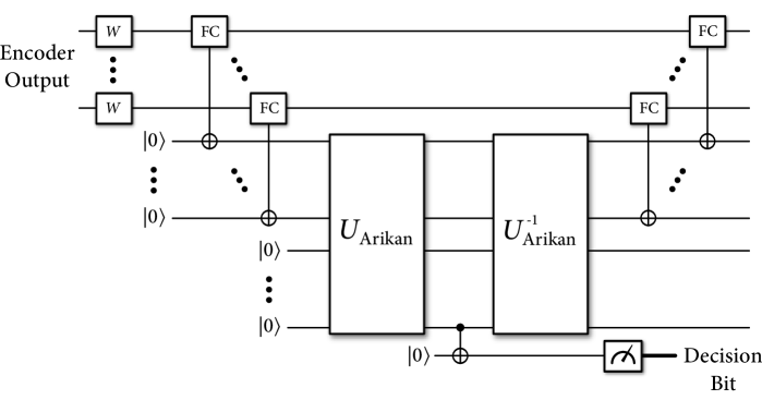
Figure 1. The circuit for recovering an information bit in the set $\mathcal{G}_{N}\mathopen{}\left(W_{\text{FC}},\beta\right)\mathclose{}$. The encoder output is fed into $N$ instances of the channel $W$. The receiver acts with $N$ of the unitaries in (53), labeled as “FC” boxes which coherently copy the likelihood ratios $\lambda_{y_{1}}$, …, $\lambda_{y_{N}}$ into ancillary registers. The receiver then acts with a reversible implementation of Arikan’s likelihood ratio computations, copies the decision bit into an ancillary register, and measures the decision bit to decode the $i^{\text{th}}$ bit. The receiver finally performs the inverse of these operations to “clean up,” i.e., to ensure that the next measurement can be performed, whether it be to decode a bit in the set $\mathcal{G}_{N}\mathopen{}\left(W_{\text{FC}},\beta\right)\mathclose{}$ or the set $\mathcal{G}_{N}\mathopen{}\left(W,\beta\right)\mathclose{}\setminus\mathcal{G}_{N}\mathopen{}\left(W_{\text{FC}},\beta\right)\mathclose{}$. The effect of this circuit is to perform the desired “gentle projection.”

For all of the remaining bits $i\in\mathcal{G}_{N}\mathopen{}\left(W,\beta\right)\mathclose{}\setminus\mathcal{G}_{N}\mathopen{}\left(W_{\text{FC}},\beta\right)\mathclose{}$, we still do not know whether there exists an efficient quantum algorithm for decoding them while having the error probability from Proposition 4.2. Thus, for now, we simply suggest for the receiver to use collective measurements to recover them.

It should be clear from Proposition 4.1 and (49) that the size of the set $\mathcal{G}_{N}\mathopen{}\left(W,\beta\right)\mathclose{}\setminus\mathcal{G}_{N}\mathopen{}\left(W_{\text{FC}},\beta\right)\mathclose{}$ in the limit is equal to

$$\lim_{N\rightarrow\infty}\frac{1}{N}\mathopen{}\left|\mathcal{G}_{N}\mathopen{}\left(W,\beta\right)\mathclose{}\setminus\mathcal{G}_{N}\mathopen{}\left(W_{\text{FC}},\beta\right)\mathclose{}\right|\mathclose{}=I\mathopen{}\left(W\right)\mathclose{}-I\mathopen{}\left(W_{\text{FC}}\right)\mathclose{}.$$ (56)

This makes it clear that one does not require a collective strategy in order to recover all of the information bits, but a collective strategy is only required in order to bridge the gap between $I\mathopen{}\left(W_{\text{FC}}\right)\mathclose{}$ and $I\mathopen{}\left(W\right)\mathclose{}$.

Observe also that similar reasoning applies to any product measurement, not just the Fuchs-Caves measurements (we focused on the Fuchs-Caves measurement due to its strong analogy with a likelihood ratio and because Arikan’s decoding algorithm processes likelihood ratios). With this in mind, we could simply choose the product measurement to be the one that maximizes the accessible information, in order to maximize the number of bits that can be processed efficiently. Let $W_{\text{acc}}$ be the classical channel induced by performing the measurement that maximizes the accessible information. One would then process the bits in $\mathcal{G}_{N}\mathopen{}\left(W_{\text{acc}},\beta\right)\mathclose{}$ in a way very similar as described above. All of the observations above then justify Claim 1.

The reasoning also leads to a generalization of Lemma 3.1 that applies when using Fuchs-Caves measurements to distinguish a tensor-product state $\rho_{0}^{\otimes N}$ from $\rho_{1}^{\otimes N}$. The test consists of performing product measurements followed by classical post-processing. If one wishes to perform this test in the most delicate way possible, one could perform it as in Figure 1.

Lemma 4.3.

When using product Fuchs-Caves measurements to distinguish $\rho_{0}^{\otimes N}$ from $\rho_{1}^{\otimes N}$, the probability of error $p_{e}$ is bounded from above in terms of the quantum fidelity $F\mathopen{}\left(\rho_{0},\rho_{1}\right)\mathclose{}$:

$$p_{e}\leq\frac{1}{2}\mathopen{}\left[F\mathopen{}\left(\rho_{0},\rho_{1}\right)\mathclose{}\right]\mathclose{}^{N}.$$ (57)

Proof 4.4.

The proof is very similar to the proof of Lemma 3.1. The test, though, consists of performing individual Fuchs-Caves measurements on the $N$ systems, and these tests result in likelihood ratios $\lambda_{y_{1}}$, …, $\lambda_{y_{N}}$. The decision rule is then as follows:

$$\text{decide\leavevmode\nobreak\ }\rho_{0}^{\otimes N}\text{ if }\lambda_{y_{1}}\times\cdots\times\lambda_{y_{N}} \geq 1,$$ (58)

$$\text{decide\leavevmode\nobreak\ }\rho_{1}^{\otimes N}\text{ if }\lambda_{y_{1}}\times\cdots\times\lambda_{y_{N}} <1.$$ (59)

An analysis proceeding exactly as in (21)-(26) leads to the following bound:

$$2\ p_{e}\mathopen{}\left(W\right)\mathclose{} \leq\sum_{y_{1},\ldots,y_{N}}\mathopen{}\left[\mathopen{}\left\langle y_{1}\right|\mathclose{}\cdots\mathopen{}\left\langle y_{N}\right|\mathclose{}\rho_{1}^{\otimes N}\mathopen{}\left|y_{1}\right\rangle\mathclose{}\cdots\mathopen{}\left|y_{N}\right\rangle\mathclose{}\right]\mathclose{}^{1/2}\ \mathopen{}\left[\mathopen{}\left\langle y_{1}\right|\mathclose{}\cdots\mathopen{}\left\langle y_{N}\right|\mathclose{}\rho_{0}^{\otimes N}\mathopen{}\left|y_{1}\right\rangle\mathclose{}\cdots\mathopen{}\left|y_{N}\right\rangle\mathclose{}\right]\mathclose{}^{1/2}$$

$$=\sum_{y_{1},\ldots,y_{N}}\mathopen{}\left\langle y_{1}\right|\mathclose{}\rho_{1}\mathopen{}\left|y_{1}\right\rangle\mathclose{}^{1/2}\ \cdots\ \mathopen{}\left\langle y_{N}\right|\mathclose{}\rho_{1}\mathopen{}\left|y_{N}\right\rangle\mathclose{}^{1/2}\ \mathopen{}\left\langle y_{1}\right|\mathclose{}\rho_{0}\mathopen{}\left|y_{1}\right\rangle\mathclose{}^{1/2}\ \cdots\ \mathopen{}\left\langle y_{N}\right|\mathclose{}\rho_{0}\mathopen{}\left|y_{N}\right\rangle\mathclose{}^{1/2}$$ (60)

$$=\sum_{y_{1}}\mathopen{}\left\langle y_{1}\right|\mathclose{}\rho_{1}\mathopen{}\left|y_{1}\right\rangle\mathclose{}^{1/2}\mathopen{}\left\langle y_{1}\right|\mathclose{}\rho_{0}\mathopen{}\left|y_{1}\right\rangle\mathclose{}^{1/2}\ \cdots\ \sum_{y_{N}}\mathopen{}\left\langle y_{N}\right|\mathclose{}\rho_{1}\mathopen{}\left|y_{N}\right\rangle\mathclose{}^{1/2}\mathopen{}\left\langle y_{N}\right|\mathclose{}\rho_{0}\mathopen{}\left|y_{N}\right\rangle\mathclose{}^{1/2}$$ (61)

$$=\mathopen{}\left[F\mathopen{}\left(\rho_{0},\rho_{1}\right)\mathclose{}\right]\mathclose{}^{N}.$$ (62)

Furthermore, one can implement this test efficiently and non-destructively on a quantum computer as described in Figure 1. The result is to project onto two different subspaces: the one spanned by eigenvectors whose corresponding eigenvalues satisfy (58) and the other.

5. Decoding the Pure-Loss Bosonic Channel

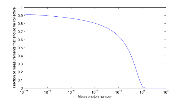
Figure 2. The fraction of collective measurements required for a polar decoder plotted as a function of the mean photon number $E$ at the receiving end, when using a BPSK coding strategy.

A channel of particular practical interest is the pure-loss bosonic channel. A simple physical model for this channel is a beamsplitter of transmissivity $\eta\in\mathopen{}\left[0,1\right]\mathclose{}$, where the sender has access to one input port, the environment injects the vacuum state into the other input port, the receiver has access to one output port, and the environment obtains the other output port. It is well known that the Holevo capacity of this channel is equal to $g\mathopen{}\left(\eta N_{S}\right)\mathclose{}\equiv\mathopen{}\left(\eta N_{S}+1\right)\mathclose{}\log\mathopen{}\left(\eta N_{S}+1\right)\mathclose{}-\eta N_{S}\log\mathopen{}\left(\eta N_{S}\right)\mathclose{}$ [6], where $N_{S}$ is the mean input photon number. In the low-photon number regime, one can come very close to achieving the capacity by employing a binary phase-shift keying (BPSK) strategy (using coherent states $\mathopen{}\left|\alpha\right\rangle\mathclose{}$ and $\mathopen{}\left|-\alpha\right\rangle\mathclose{}$ as the signaling states) [21]. The BPSK strategy induces a cq channel of the following form: $x\rightarrow\mathopen{}\left|\mathopen{}\left(-1\right)\mathclose{}^{x}\alpha\right\rangle\mathclose{}\mathopen{}\left\langle\mathopen{}\left(-1\right)\mathclose{}^{x}\alpha\right|\mathclose{}$. The symmetric Holevo rate for this channel is equal to $\chi\mathopen{}\left(E\right)\mathclose{}\equiv h_{2}\mathopen{}\left(\mathopen{}\left[1+e^{-2E}\right]\mathclose{}/2\right)\mathclose{}$, where $h_{2}$ is the binary entropy and $E\equiv\eta N_{S}$. If the receiver performs a Helstrom measurement at every channel output, this induces a classical channel with symmetric mutual information equal to $I_{\text{Hel}}\mathopen{}\left(E\right)\mathclose{}\equiv 1-h_{2}([1-\sqrt{1-e^{-4E}}]/2)$. (See Ref. [9], for example, for explicit calculations.) Our results in the previous section demonstrate that the fraction of information bits required to be decoded using a collective strategy is equal to $1-I_{\text{Hel}}\mathopen{}\left(E\right)\mathclose{}/\chi\mathopen{}\left(E\right)\mathclose{}$. Figure 2 reveals that this fraction is rather small for mean photon number (MPN) larger than one, but then it rises sharply as we enter a quantum regime where the MPN is less than one. Even deep in the quantum regime at a MPN of $10^{-8}$, however, roughly 10% of the bits do not require collective decoding.

6. Small Blocklength Polar Decoders

This section briefly discusses how the Helstrom measurements [12, 13] in the quantum successive cancellation decoder from Ref. [23] decompose for very small size polar codes.

6.1. Two-Bit Polar Decoder

We begin by considering the simple two-bit polar code. The channel is of the form $x\rightarrow\rho_{x}$, where $x\in\mathopen{}\left\{0,1\right\}\mathclose{}$ and $\rho_{x}$ is some conditional density operator. The two-bit polar code performs the simple transformation on the input bits $u_{1}$ and $u_{2}$:

$$\mathopen{}\left(u_{1},u_{2}\right)\mathclose{}\rightarrow\mathopen{}\left(u_{1}+u_{2},u_{2}\right)\mathclose{},$$ (63)

where addition is modulo 2.

The first step of the successive cancellation decoder is to recover $u_{1}$, assuming that bit $u_{2}$ is chosen uniformly at random. The optimal measurement is a Helstrom measurement, and in this case, it amounts to distinguishing between the following two states

$$\frac{1}{2}\sum_{u_{2}}\rho_{u_{2}}\otimes\rho_{u_{2}},\ \ \ \ \ \ \ \frac{1}{2}\sum_{u_{2}}\rho_{u_{2}+1}\otimes\rho_{u_{2}}.$$ (64)

The Helstrom measurement is given by the projector onto the positive eigenspace of the difference of the two density operators above:

$$\mathopen{}\left\{\frac{1}{2}\sum_{u_{2}}\rho_{u_{2}}\otimes\rho_{u_{2}}-\frac{1}{2}\sum_{u_{2}}\rho_{u_{2}+1}\otimes\rho_{u_{2}}\geq 0\right\}\mathclose{} =\mathopen{}\left\{\sum_{u_{2}}\mathopen{}\left(\rho_{u_{2}}-\rho_{u_{2}+1}\right)\mathclose{}\otimes\rho_{u_{2}}\geq 0\right\}\mathclose{}$$ (65)

$$=\mathopen{}\left\{\sum_{u_{2}}\mathopen{}\left(-1\right)\mathclose{}^{u_{2}}\mathopen{}\left(\rho_{0}-\rho_{1}\right)\mathclose{}\otimes\rho_{u_{2}}\geq 0\right\}\mathclose{}$$ (66)

$$=\mathopen{}\left\{\mathopen{}\left(\rho_{0}-\rho_{1}\right)\mathclose{}\otimes\sum_{u_{2}}\mathopen{}\left(-1\right)\mathclose{}^{u_{2}}\rho_{u_{2}}\geq 0\right\}\mathclose{}$$ (67)

$$=\mathopen{}\left\{\mathopen{}\left(\rho_{0}-\rho_{1}\right)\mathclose{}\otimes\mathopen{}\left(\rho_{0}-\rho_{1}\right)\mathclose{}\geq 0\right\}\mathclose{}.$$ (68)

Thus, this test factorizes into the parity of the individual quantum hypothesis tests $\mathopen{}\left\{\mathopen{}\left(\rho_{0}-\rho_{1}\right)\mathclose{}\geq 0\right\}\mathclose{}$. That is, supposing that $\Pi_{+}\equiv\mathopen{}\left\{\mathopen{}\left(\rho_{0}-\rho_{1}\right)\mathclose{}\geq 0\right\}\mathclose{}$ and $\Pi_{-}\equiv\mathopen{}\left\{\mathopen{}\left(\rho_{0}-\rho_{1}\right)\mathclose{}<0\right\}\mathclose{}$, one can write the two-bit test as the product of two controlled gates

$$U_{1} \equiv I_{B_{1}}\otimes\mathopen{}\left(\Pi_{+}\right)\mathclose{}_{B_{2}}\otimes I_{A}+I_{B_{1}}\otimes\mathopen{}\left(\Pi_{-}\right)\mathclose{}_{B_{2}}\otimes\mathopen{}\left(\sigma_{X}\right)\mathclose{}_{A},$$ (69)

$$U_{2} \equiv\mathopen{}\left(\Pi_{+}\right)\mathclose{}_{B_{1}}\otimes I_{B_{2}}\otimes I_{A}+\mathopen{}\left(\Pi_{-}\right)\mathclose{}_{B_{1}}\otimes I_{B_{2}}\otimes\mathopen{}\left(\sigma_{X}\right)\mathclose{}_{A},$$ (70)

where $B_{1}$ is the first channel output, $B_{2}$ is the second channel output, and $A$ is an ancillary system initialized to the state $\mathopen{}\left|0\right\rangle\mathclose{}$. The product of these two unitary gates is equal to

$$U_{1}U_{2}=\mathopen{}\left(\mathopen{}\left(\Pi_{+}\right)\mathclose{}_{B_{1}}\otimes\mathopen{}\left(\Pi_{+}\right)\mathclose{}_{B_{2}}+\mathopen{}\left(\Pi_{-}\right)\mathclose{}_{B_{1}}\otimes\mathopen{}\left(\Pi_{-}\right)\mathclose{}_{B_{2}}\right)\mathclose{}\otimes I_{A}+\\ \mathopen{}\left(\mathopen{}\left(\Pi_{-}\right)\mathclose{}_{B_{1}}\otimes\mathopen{}\left(\Pi_{+}\right)\mathclose{}_{B_{2}}+\mathopen{}\left(\Pi_{+}\right)\mathclose{}_{B_{1}}\otimes\mathopen{}\left(\Pi_{-}\right)\mathclose{}_{B_{2}}\right)\mathclose{}\otimes\mathopen{}\left(\sigma_{X}\right)\mathclose{}_{A}.$$ (71)

The receiver would then measure the ancillary system $A$ in order to make a decision about $u_{1}$.

Next, we determine the decoding of $u_{2}$, given that $u_{1}$ has already been decoded. By the definition of the polar encoder transformation in (63), the goal is to distinguish between the following two states:

$$\rho_{u_{1}}\otimes\rho_{0},\ \ \ \ \ \ \ \rho_{u_{1}+1}\otimes\rho_{1}.$$ (72)

The optimal quantum hypothesis test is given by the following projector:

$$\mathopen{}\left\{\rho_{u_{1}}\otimes\rho_{0}-\rho_{u_{1}+1}\otimes\rho_{1}\geq 0\right\}\mathclose{}.$$ (73)

This optimal quantum hypothesis test is not factorizable into smaller tests, and indeed, it is necessary to perform a collective measurement in order to implement it. Nonetheless, Lemma 4.3 provides a simple implementation of the Fuchs-Caves measurement for distinguishing these two states.

6.2. Four-Bit Polar Decoder

We now consider the form of Helstrom measurements for a four-bit polar code. Recall that the input transformation for the four-bit polar code is as follows:

$$\mathopen{}\left(u_{1},u_{2},u_{3},u_{4}\right)\mathclose{}\rightarrow\mathopen{}\left(u_{1}+u_{2}+u_{3}+u_{4},u_{3}+u_{4},u_{2}+u_{4},u_{4}\right)\mathclose{}.$$ (74)

It is straightforward to find the form of the four different tests for decoding $u_{1}$ through $u_{4}$. (See the appendix for derivations.) The test for decoding $u_{1}$ is again a parity test:

$$\mathopen{}\left\{\mathopen{}\left(\rho_{0}-\rho_{1}\right)\mathclose{}^{\otimes 4}\geq 0\right\}\mathclose{}.$$ (75)

The test for decoding $u_{2}$ given $u_{1}$ is

$$\mathopen{}\left\{\mathopen{}\left(\sum_{u_{3}^{\prime}}\rho_{u_{1}+u_{3}^{\prime}}\otimes\rho_{u_{3}^{\prime}}\right)\mathclose{}\otimes\mathopen{}\left(\sum_{u_{4}}\rho_{u_{4}}\otimes\rho_{u_{4}}\right)\mathclose{}-\mathopen{}\left(\sum_{u_{3}^{\prime}}\rho_{u_{1}+1+u_{3}^{\prime}}\otimes\rho_{u_{3}^{\prime}}\right)\mathclose{}\otimes\mathopen{}\left(\sum_{u_{4}}\rho_{1+u_{4}}\otimes\rho_{u_{4}}\right)\mathclose{}\geq 0\right\}\mathclose{}.$$ (76)

It remains unclear to us if there is a simple way to decompose the above test any further into non-collective actions (or even approximately using, e.g., the Fuchs-Caves measurement). The test for decoding $u_{3}$ given $u_{2}$ and $u_{1}$ is

$$\mathopen{}\left\{\mathopen{}\left(\rho_{u_{1}+u_{2}}\otimes\rho_{0}-\rho_{u_{1}+u_{2}+1}\otimes\rho_{1}\right)\mathclose{}\otimes\mathopen{}\left(\rho_{u_{2}}\otimes\rho_{0}-\rho_{u_{2}+1}\otimes\rho_{1}\right)\mathclose{}\geq 0\right\}\mathclose{}.$$ (77)

One could actually approximate this test “efficiently” by performing a product Fuchs-Caves measurement of the first two systems, a product Fuchs-Caves measurement of the last two, and then take the parity of the results of these two tests (of course implementing these tests coherently). The final Helstrom test for decoding $u_{4}$ given $u_{3}$, $u_{2}$, and $u_{1}$ is

$$\mathopen{}\left\{\rho_{u_{1}+u_{2}+u_{3}}\otimes\rho_{u_{3}}\otimes\rho_{u_{2}}\otimes\rho_{0}-\rho_{u_{1}+u_{2}+u_{3}+1}\otimes\rho_{u_{3}+1}\otimes\rho_{u_{2}+1}\otimes\rho_{1}\geq 0\right\}\mathclose{}.$$ (78)

Clearly, it would be better to perform this last test by processing the likelihood ratios resulting from individual Fuchs-Caves measurements, rather than performing the optimal collective Helstrom measurement.

6.3. Polar Decoder for Larger Blocklengths

One can continue in the above fashion to determine the form of a quantum successive cancellation decoder that recovers each bit of an eight-bit polar code. We again try to simplify each Helstrom measurement and provide an expression for each one in Appendix B. A few tests simplify, in particular those used to recover the first bit $u_{1}$ (Eq. (101)), the fifth bit $u_{5}$ (Eq. (112), the seventh bit $u_{7}$ (Eq. (115)), and the last bit $u_{8}$ (Eq. (117)). However, for the other tests, it is unclear if they can be approximated by some combination of Helstrom and Fuchs-Caves measurements, followed by coherent post-processing.

From considering the eight-bit polar decoder, we can make several observations. For any blocklength, it is always possible to recover the first bit efficiently by calculating the parity of individual Helstrom measurements (though, this bit is always the “worst” bit, so the receiver would never actually be decoding it in practice). The receiver can always recover the last bit by performing a Fuchs-Caves measurement (this is always the “best” bit, so this should already be evident from the main observation in this paper). Furthermore, there are many bits that can be recovered by first performing Fuchs-Caves measurements, followed by the parity of these tests. Unfortunately, the fraction of these tests tends to zero in the limit of large blocklength. Thus, there still remains much to understand regarding the structure of a polar decoder.

7. Conclusion

The main result of this paper is an advance over previous schemes for decoding classical information transmitted over channels with classical inputs and quantum outputs. In particular, we have shown that $N\cdot I\mathopen{}\left(W_{\text{acc}}\right)\mathclose{}$ of the information bits can be decoded reliably and efficiently on a quantum computer by a “non-collective” coherent decoding strategy, while closing the gap to the Holevo information rate (decoding the other $N\mathopen{}\left(I\mathopen{}\left(W\right)\mathclose{}-I\mathopen{}\left(W_{\text{acc}}\right)\mathclose{}\right)\mathclose{}$ bits) should require a collective strategy. For the pure-loss bosonic channel, this implies that the majority of the bits transmitted can be decoded by a product strategy whenever the mean photon number is larger than one, while the fraction of collective measurements required increases sharply as the mean photon number decreases below one, marking the beginning of the quantum regime. Remarkably, even at mean photon numbers as low as $10^{-8}$, roughly 10% of the bits do not require collective decoding, however. As another contribution, we have shown that a receiver can also employ collective Fuchs-Caves measurements when decoding a classical-quantum polar code. Finally, we gave the explicit form of the Helstrom measurements of a quantum successive cancellation decoder for two-, four-, and eight-bit polar codes. This should be helpful in determining the explicit form of tests for larger blocklength polar codes.

The main open question is still to determine whether all of the information bits can be efficiently decoded on a quantum computer. To answer this question, one might consider employing the Schur transform [3, 10, 4] and exploiting the structure inherent in polar codes. Unfortunately, it is not clear to us that this approach will lead to a quantum successive cancellation decoder with time complexity $O\mathopen{}\left(N\log N\right)\mathclose{}$ because the complexity of the Schur transform is higher than this.

We acknowledge helpful discussions with Frédéric Dupuis, Saikat Guha, Hari Krovi, David Poulin, and Joseph Renes. MMW acknowledges support from Montreal’s Centre de Recherches Mathématiques. OLC aknowledges support from NSERC through a Vanier scholarship. PH acknowledges support from the Canada Research Chairs program, the Perimeter Institute, CIFAR, FQRNT’s INTRIQ, NSERC, and ONR through grant N000140811249.

Appendix A Derivations for the Four-Bit Polar Decoder Measurements

The four-bit polar encoder amounts to the following transformation:

$$\mathopen{}\left(u_{1},u_{2},u_{3},u_{4}\right)\mathclose{}\rightarrow\mathopen{}\left(u_{1}+u_{2}+u_{3}+u_{4},u_{3}+u_{4},u_{2}+u_{4},u_{4}\right)\mathclose{}.$$ (79)

A.1. Recovering $u_{1}$

Let us first determine how the quantum successive cancellation decoder (QSCD) recovers the bit $u_{1}$, assuming that $u_{2}$, $u_{3}$, and $u_{4}$ are chosen uniformly at random. The test aims to distinguish between the following two states:

$$\frac{1}{2^{3}}\sum_{u_{2},u_{3},u_{4}}\rho_{u_{2}+u_{3}+u_{4}}\otimes\rho_{u_{3}+u_{4}}\otimes\rho_{u_{2}+u_{4}}\otimes\rho_{u_{4}},$$ (80)

$$\frac{1}{2^{3}}\sum_{u_{2},u_{3},u_{4}}\rho_{u_{2}+u_{3}+u_{4}+1}\otimes\rho_{u_{3}+u_{4}}\otimes\rho_{u_{2}+u_{4}}\otimes\rho_{u_{4}},$$ (81)

and it performs the following projection:

$$\mathopen{}\left\{\sum_{u_{2},u_{3},u_{4}}\mathopen{}\left(\rho_{u_{2}+u_{3}+u_{4}}-\rho_{u_{2}+u_{3}+u_{4}+1}\right)\mathclose{}\otimes\rho_{u_{3}+u_{4}}\otimes\rho_{u_{2}+u_{4}}\otimes\rho_{u_{4}}\geq 0\right\}\mathclose{}$$

$$=\mathopen{}\left\{\sum_{u_{2},u_{3},u_{4}}\mathopen{}\left(-1\right)\mathclose{}^{u_{2}+u_{3}+u_{4}}\mathopen{}\left(\rho_{0}-\rho_{1}\right)\mathclose{}\otimes\rho_{u_{3}+u_{4}}\otimes\rho_{u_{2}+u_{4}}\otimes\rho_{u_{4}}\geq 0\right\}\mathclose{}$$ (82)

$$=\mathopen{}\left\{\mathopen{}\left(\rho_{0}-\rho_{1}\right)\mathclose{}\otimes\sum_{u_{2},u_{3},u_{4}}\mathopen{}\left(-1\right)\mathclose{}^{u_{2}+u_{3}+u_{4}}\rho_{u_{3}+u_{4}}\otimes\rho_{u_{2}+u_{4}}\otimes\rho_{u_{4}}\geq 0\right\}\mathclose{}$$ (83)

$$=\mathopen{}\left\{\mathopen{}\left(\rho_{0}-\rho_{1}\right)\mathclose{}\otimes\sum_{u_{2},u_{3},u_{4}}\mathopen{}\left(-1\right)\mathclose{}^{u_{3}+u_{4}}\rho_{u_{3}+u_{4}}\otimes\mathopen{}\left(-1\right)\mathclose{}^{u_{2}+u_{4}}\rho_{u_{2}+u_{4}}\otimes\mathopen{}\left(-1\right)\mathclose{}^{u_{4}}\rho_{u_{4}}\geq 0\right\}\mathclose{}$$ (84)

$$=\mathopen{}\left\{\mathopen{}\left(\rho_{0}-\rho_{1}\right)\mathclose{}\otimes\sum_{u_{2}^{\prime},u_{3}^{\prime},u_{4}^{\prime}}\mathopen{}\left(-1\right)\mathclose{}^{u_{2}^{\prime}}\rho_{u_{2}^{\prime}}\otimes\mathopen{}\left(-1\right)\mathclose{}^{u_{3}^{\prime}}\rho_{u_{3}^{\prime}}\otimes\mathopen{}\left(-1\right)\mathclose{}^{u_{4}^{\prime}}\rho_{u_{4}^{\prime}}\geq 0\right\}\mathclose{}$$ (85)

$$=\mathopen{}\left\{\mathopen{}\left(\rho_{0}-\rho_{1}\right)\mathclose{}\otimes\sum_{u_{2}^{\prime}}\mathopen{}\left(-1\right)\mathclose{}^{u_{2}^{\prime}}\rho_{u_{2}^{\prime}}\otimes\sum_{u_{3}^{\prime}}\mathopen{}\left(-1\right)\mathclose{}^{u_{3}^{\prime}}\rho_{u_{3}^{\prime}}\otimes\sum_{u_{4}^{\prime}}\mathopen{}\left(-1\right)\mathclose{}^{u_{4}^{\prime}}\rho_{u_{4}^{\prime}}\geq 0\right\}\mathclose{}$$ (86)

$$=\mathopen{}\left\{\mathopen{}\left(\rho_{0}-\rho_{1}\right)\mathclose{}\otimes\mathopen{}\left(\rho_{0}-\rho_{1}\right)\mathclose{}\otimes\mathopen{}\left(\rho_{0}-\rho_{1}\right)\mathclose{}\otimes\mathopen{}\left(\rho_{0}-\rho_{1}\right)\mathclose{}\geq 0\right\}\mathclose{}.$$ (87)

Thus, this first test nicely factors as the parity of the four individual tests $\mathopen{}\left\{\mathopen{}\left(\rho_{0}-\rho_{1}\right)\mathclose{}\geq 0\right\}\mathclose{}$.

A.2. Recovering $u_{2}$ given $u_{1}$

We now determine how the quantum successive cancellation decoder recovers $u_{2}$ given $u_{1}$, while randomizing over $u_{3}$ and $u_{4}$. The aim is to distinguish between the following two states:

$$\frac{1}{2^{2}}\sum_{u_{3},u_{4}}\rho_{u_{1}+u_{3}+u_{4}}\otimes\rho_{u_{3}+u_{4}}\otimes\rho_{u_{4}}\otimes\rho_{u_{4}},$$ (88)

$$\frac{1}{2^{2}}\sum_{u_{3},u_{4}}\rho_{u_{1}+1+u_{3}+u_{4}}\otimes\rho_{u_{3}+u_{4}}\otimes\rho_{1+u_{4}}\otimes\rho_{u_{4}},$$ (89)

which translates to a projection of the following form:

$$\mathopen{}\left\{\sum_{u_{3},u_{4}}\rho_{u_{1}+u_{3}+u_{4}}\otimes\rho_{u_{3}+u_{4}}\otimes\rho_{u_{4}}\otimes\rho_{u_{4}}-\rho_{u_{1}+1+u_{3}+u_{4}}\otimes\rho_{u_{3}+u_{4}}\otimes\rho_{1+u_{4}}\otimes\rho_{u_{4}}\geq 0\right\}\mathclose{}.$$ (90)

Define $u_{3}^{\prime}=u_{3}+u_{4}$ and the above becomes

$$\mathopen{}\left\{\sum_{u_{3}^{\prime},u_{4}}\rho_{u_{1}+u_{3}^{\prime}}\otimes\rho_{u_{3}^{\prime}}\otimes\rho_{u_{4}}\otimes\rho_{u_{4}}-\rho_{u_{1}+1+u_{3}^{\prime}}\otimes\rho_{u_{3}^{\prime}}\otimes\rho_{1+u_{4}}\otimes\rho_{u_{4}}\geq 0\right\}\mathclose{}$$

$$=\mathopen{}\left\{\mathopen{}\left(\sum_{u_{3}^{\prime}}\rho_{u_{1}+u_{3}^{\prime}}\otimes\rho_{u_{3}^{\prime}}\right)\mathclose{}\otimes\mathopen{}\left(\sum_{u_{4}}\rho_{u_{4}}\otimes\rho_{u_{4}}\right)\mathclose{}-\mathopen{}\left(\sum_{u_{3}^{\prime}}\rho_{u_{1}+1+u_{3}^{\prime}}\otimes\rho_{u_{3}^{\prime}}\right)\mathclose{}\otimes\mathopen{}\left(\sum_{u_{4}}\rho_{1+u_{4}}\otimes\rho_{u_{4}}\right)\mathclose{}\geq 0\right\}\mathclose{}.$$ (91)

A.3. Recovering $u_{3}$ given $u_{2}$ and $u_{1}$

Let us determine how the QSCD recovers $u_{3}$ given $u_{2}$ and $u_{1}$, while randomizing over $u_{4}$. The test distinguishes between the following two states:

$$\frac{1}{2}\sum_{u_{4}}\rho_{u_{1}+u_{2}+u_{4}}\otimes\rho_{u_{4}}\otimes\rho_{u_{2}+u_{4}}\otimes\rho_{u_{4}},$$ (92)

$$\frac{1}{2}\sum_{u_{4}}\rho_{u_{1}+u_{2}+1+u_{4}}\otimes\rho_{1+u_{4}}\otimes\rho_{u_{2}+u_{4}}\otimes\rho_{u_{4}},$$ (93)

and amounts to a projector of the following form:

$$\mathopen{}\left\{\sum_{u_{4}}\rho_{u_{1}+u_{2}+u_{4}}\otimes\rho_{u_{4}}\otimes\rho_{u_{2}+u_{4}}\otimes\rho_{u_{4}}-\sum_{u_{4}}\rho_{u_{1}+u_{2}+1+u_{4}}\otimes\rho_{1+u_{4}}\otimes\rho_{u_{2}+u_{4}}\otimes\rho_{u_{4}}\geq 0\right\}\mathclose{}$$

$$=\mathopen{}\left\{\sum_{u_{4}}\mathopen{}\left(\rho_{u_{1}+u_{2}+u_{4}}\otimes\rho_{u_{4}}-\rho_{u_{1}+u_{2}+1+u_{4}}\otimes\rho_{1+u_{4}}\right)\mathclose{}\otimes\rho_{u_{2}+u_{4}}\otimes\rho_{u_{4}}\geq 0\right\}\mathclose{}$$ (94)

$$=\mathopen{}\left\{\sum_{u_{4}}\mathopen{}\left(-1\right)\mathclose{}^{u_{4}}\mathopen{}\left(\rho_{u_{1}+u_{2}}\otimes\rho_{0}-\rho_{u_{1}+u_{2}+1}\otimes\rho_{1}\right)\mathclose{}\otimes\rho_{u_{2}+u_{4}}\otimes\rho_{u_{4}}\geq 0\right\}\mathclose{}$$ (95)

$$=\mathopen{}\left\{\mathopen{}\left(\rho_{u_{1}+u_{2}}\otimes\rho_{0}-\rho_{u_{1}+u_{2}+1}\otimes\rho_{1}\right)\mathclose{}\otimes\sum_{u_{4}}\mathopen{}\left(-1\right)\mathclose{}^{u_{4}}\rho_{u_{2}+u_{4}}\otimes\rho_{u_{4}}\geq 0\right\}\mathclose{}$$ (96)

$$=\mathopen{}\left\{\mathopen{}\left(\rho_{u_{1}+u_{2}}\otimes\rho_{0}-\rho_{u_{1}+u_{2}+1}\otimes\rho_{1}\right)\mathclose{}\otimes\mathopen{}\left(\rho_{u_{2}}\otimes\rho_{0}-\rho_{u_{2}+1}\otimes\rho_{1}\right)\mathclose{}\geq 0\right\}\mathclose{}.$$ (97)

Thus, this test nicely factorizes as the parity of two tests $\mathopen{}\left\{\mathopen{}\left(\rho_{u_{1}+u_{2}}\otimes\rho_{0}-\rho_{u_{1}+u_{2}+1}\otimes\rho_{1}\right)\mathclose{}\geq 0\right\}\mathclose{}$ and $\mathopen{}\left\{\mathopen{}\left(\rho_{u_{2}}\otimes\rho_{0}-\rho_{u_{2}+1}\otimes\rho_{1}\right)\mathclose{}\geq 0\right\}\mathclose{}$.

A.4. Recovering $u_{4}$ given $u_{3}$, $u_{2}$, and $u_{1}$

Finally, we determine how the QSCD recovers $u_{4}$ given all of the previous bits. The test in this case just aims to distinguish the following states:

$$\rho_{u_{1}+u_{2}+u_{3}}\otimes\rho_{u_{3}}\otimes\rho_{u_{2}}\otimes\rho_{0},$$ (98)

$$\rho_{u_{1}+u_{2}+u_{3}+1}\otimes\rho_{u_{3}+1}\otimes\rho_{u_{2}+1}\otimes\rho_{1},$$ (99)

and amounts to the following projection:

$$\mathopen{}\left\{\rho_{u_{1}+u_{2}+u_{3}}\otimes\rho_{u_{3}}\otimes\rho_{u_{2}}\otimes\rho_{0}-\rho_{u_{1}+u_{2}+u_{3}+1}\otimes\rho_{u_{3}+1}\otimes\rho_{u_{2}+1}\otimes\rho_{1}\geq 0\right\}\mathclose{}.$$ (100)

Appendix B Measurements for the Eight-Bit Polar Decoder

Here, we provide the form of a quantum successive cancellation decoder that recovers each bit of an eight-bit polar code. Full derivations of the results in this section are available from the authors upon request.

B.1. Recovering $u_{1}$

The test to recover the first bit $u_{1}$ is simply the parity of eight individual Helstrom measurements:

$$\mathopen{}\left\{\mathopen{}\left(\rho_{0}-\rho_{1}\right)\mathclose{}^{\otimes 8}\geq 0\right\}\mathclose{}.$$ (101)

B.2. Recovering $u_{2}$ given $u_{1}$

The test to recover bit $u_{2}$ given $u_{1}$ projects onto the positive eigenspace of the difference of

$$\mathopen{}\left(\sum_{u_{3}^{\prime},u_{4}^{\prime},u_{5}^{\prime}}\rho_{u_{1}+u_{3}^{\prime}+u_{4}^{\prime}+u_{5}^{\prime}}\otimes\rho_{u_{3}^{\prime}}\otimes\rho_{u_{4}^{\prime}}\otimes\rho_{u_{5}^{\prime}}\right)\mathclose{}\otimes\mathopen{}\left(\sum_{u_{6}^{\prime},u_{7}^{\prime},u_{8}^{\prime}}\rho_{u_{6}^{\prime}+u_{7}^{\prime}+u_{8}^{\prime}}\otimes\rho_{u_{6}^{\prime}}\otimes\rho_{u_{7}^{\prime}}\otimes\rho_{u_{8}^{\prime}}\right)\mathclose{}$$ (102)

and

$$\mathopen{}\left(\sum_{u_{3}^{\prime},u_{4}^{\prime},u_{5}^{\prime}}\rho_{u_{1}+u_{3}^{\prime}+u_{4}^{\prime}+u_{5}^{\prime}}\otimes\rho_{u_{3}^{\prime}}\otimes\rho_{u_{4}^{\prime}}\otimes\rho_{u_{5}^{\prime}}\right)\mathclose{}\otimes\mathopen{}\left(\sum_{u_{6}^{\prime},u_{7}^{\prime},u_{8}^{\prime}}\rho_{u_{6}^{\prime}+u_{7}^{\prime}+u_{8}^{\prime}}\otimes\rho_{u_{6}^{\prime}}\otimes\rho_{u_{7}^{\prime}}\otimes\rho_{u_{8}^{\prime}}\right)\mathclose{}.$$ (103)

As such, it is not clear to us how one could approximate this test as some combination of Helstrom and Fuchs-Caves tests.

B.3. Recovering $u_{3}$ given $u_{2}$, and $u_{1}$

The test to recover bit $u_{3}$ given $u_{1}$ and $u_{2}$ is equal to the parity of the following two tests:

$$\mathopen{}\left\{\begin{array}[c]{c}\mathopen{}\left(\sum_{u_{4}^{\prime}}\rho_{u_{1}+u_{2}+u_{4}^{\prime}}\otimes\rho_{u_{4}^{\prime}}\right)\mathclose{}\otimes\mathopen{}\left(\sum_{u_{5}^{\prime}}\rho_{u_{5}^{\prime}}\otimes\rho_{u_{5}^{\prime}}\right)\mathclose{}\\ -\mathopen{}\left(\sum_{u_{4}^{\prime}}\rho_{u_{1}+u_{2}+1+u_{4}^{\prime}}\otimes\rho_{u_{4}^{\prime}}\right)\mathclose{}\otimes\mathopen{}\left(\sum_{u_{5}^{\prime}}\rho_{1+u_{5}^{\prime}}\otimes\rho_{u_{5}^{\prime}}\right)\mathclose{}\geq 0\end{array}\right\}\mathclose{},$$ (106)

$$\mathopen{}\left\{\begin{array}[c]{c}\mathopen{}\left(\sum_{u_{6}^{\prime}}\rho_{u_{2}+u_{6}^{\prime}}\otimes\rho_{u_{6}^{\prime}}\right)\mathclose{}\otimes\mathopen{}\left(\sum_{u_{8}^{\prime\prime}}\rho_{u_{8}^{\prime\prime}}\otimes\rho_{u_{8}^{\prime\prime}}\right)\mathclose{}\\ -\mathopen{}\left(\sum_{u_{6}^{\prime}}\rho_{u_{2}+u_{6}^{\prime}+1}\otimes\rho_{u_{6}^{\prime}}\right)\mathclose{}\otimes\mathopen{}\left(\sum_{u_{8}^{\prime\prime}}\rho_{1+u_{8}^{\prime\prime}}\otimes\rho_{u_{8}^{\prime\prime}}\right)\mathclose{}\geq 0\end{array}\right\}\mathclose{}.$$ (109)

It is again unclear to us how to decompose this measurement further.

B.4. Recovering $u_{4}$ given $u_{3}$, $u_{2}$, and $u_{1}$

The test to recover bit $u_{4}$ given $u_{1}$, $u_{2}$, and $u_{3}$ projects onto the positive eigenspace of the difference of

$$\mathopen{}\left(\sum_{u_{5}^{\prime}}\rho_{u_{1}+u_{2}+u_{3}+u_{5}^{\prime}}\otimes\rho_{u_{5}^{\prime}}\right)\mathclose{}\otimes\mathopen{}\left(\sum_{u_{6}^{\prime}}\rho_{u_{3}+u_{6}^{\prime}}\otimes\rho_{u_{6}^{\prime}}\right)\mathclose{}\otimes\mathopen{}\left(\sum_{u_{7}^{\prime}}\rho_{u_{2}+u_{7}^{\prime}}\otimes\rho_{u_{7}^{\prime}}\right)\mathclose{}\otimes\mathopen{}\left(\sum_{u_{8}^{\prime}}\rho_{u_{8}^{\prime}}\otimes\rho_{u_{8}^{\prime}}\right)\mathclose{}$$ (110)

and

$$\mathopen{}\left(\sum_{u_{5}^{\prime}}\rho_{u_{1}+u_{2}+u_{3}+1+u_{5}^{\prime}}\otimes\rho_{u_{5}^{\prime}}\right)\mathclose{}\otimes\mathopen{}\left(\sum_{u_{6}^{\prime}}\rho_{u_{3}+1+u_{6}^{\prime}}\otimes\rho_{u_{6}^{\prime}}\right)\mathclose{}\otimes\mathopen{}\left(\sum_{u_{7}^{\prime}}\rho_{u_{2}+1+u_{7}^{\prime}}\otimes\rho_{u_{7}^{\prime}}\right)\mathclose{}\otimes\mathopen{}\left(\sum_{u_{8}^{\prime}}\rho_{1+u_{8}^{\prime}}\otimes\rho_{u_{8}^{\prime}}\right)\mathclose{}$$ (111)

Again, this one remains unclear how to decompose further.

B.5. Recovering $u_{5}$ given $u_{4}$, …, $u_{1}$

The test to recover bit $u_{5}$ given $u_{1}$ through $u_{4}$ is equal to

$$\mathopen{}\left\{\begin{array}[c]{c}\mathopen{}\left(\rho_{u_{1}+u_{2}+u_{3}+u_{4}}\otimes\rho_{0}-\rho_{u_{1}+u_{2}+u_{3}+u_{4}+1}\otimes\rho_{1}\right)\mathclose{}\otimes\mathopen{}\left(\rho_{u_{3}+u_{4}}\otimes\rho_{0}-\rho_{u_{3}+u_{4}+1}\otimes\rho_{1}\right)\mathclose{}\\ \otimes\mathopen{}\left(\rho_{u_{2}+u_{4}}\otimes\rho_{0}-\rho_{u_{2}+u_{4}+1}\otimes\rho_{1}\right)\mathclose{}\otimes\mathopen{}\left(\rho_{u_{4}}\otimes\rho_{0}-\rho_{u_{4}+1}\otimes\rho_{1}\right)\mathclose{}\geq 0\end{array}\right\}\mathclose{}.$$ (112)

It is easy to see that one could approximate this test by first performing four Fuchs-Caves measurements on adjacent pairs of channel outputs and taking the parity of these tests.

B.6. Recovering $u_{6}$ given $u_{5}$, …, $u_{1}$

The test to recover bit $u_{6}$ given $u_{1}$ through $u_{5}$ is a projection onto the positive eigenspace of the difference of

$$\mathopen{}\left(\sum_{u_{7}^{\prime}}\rho_{u_{1}+\cdots+u_{5}+u_{7}^{\prime}}\otimes\rho_{u_{5}+u_{7}^{\prime}}\otimes\rho_{u_{3}+u_{4}+u_{7}^{\prime}}\otimes\rho_{u_{7}^{\prime}}\right)\mathclose{}\otimes\mathopen{}\left(\sum_{u_{8}^{\prime}}\rho_{u_{2}+u_{4}+u_{8}^{\prime}}\otimes\rho_{u_{8}^{\prime}}\otimes\rho_{u_{4}+u_{8}^{\prime}}\otimes\rho_{u_{8}^{\prime}}\right)\mathclose{}$$ (113)

and

$$\mathopen{}\left(\sum_{u_{7}^{\prime}}\rho_{u_{1}+\cdots+u_{5}+1+u_{7}^{\prime}}\otimes\rho_{u_{5}+1+u_{7}^{\prime}}\otimes\rho_{u_{3}+u_{4}+u_{7}^{\prime}}\otimes\rho_{u_{7}^{\prime}}\right)\mathclose{}\otimes\mathopen{}\left(\sum_{u_{8}^{\prime}}\rho_{u_{2}+u_{4}+1+u_{8}^{\prime}}\otimes\rho_{1+u_{8}^{\prime}}\otimes\rho_{u_{4}+u_{8}^{\prime}}\otimes\rho_{u_{8}^{\prime}}\right)\mathclose{}.$$ (114)

A simple decomposition of this test remains unclear.

B.7. Recovering $u_{7}$ given $u_{6}$, …, $u_{1}$

The test for recovering bit $u_{7}$ given the previous ones is

$$\mathopen{}\left\{\begin{array}[c]{c}\mathopen{}\left(\rho_{u_{1}+\cdots+u_{6}}\otimes\rho_{u_{5}+u_{6}}\otimes\rho_{u_{3}+u_{4}}\otimes\rho_{0}-\rho_{u_{1}+\cdots+u_{6}+1}\otimes\rho_{u_{5}+u_{6}+1}\otimes\rho_{u_{3}+u_{4}+1}\otimes\rho_{1}\right)\mathclose{}\otimes\\ \mathopen{}\left(\rho_{u_{2}+u_{4}+u_{6}}\otimes\rho_{u_{6}}\otimes\rho_{u_{4}}\otimes\rho_{0}-\rho_{u_{2}+u_{4}+u_{6}+1}\otimes\rho_{u_{6}+1}\otimes\rho_{u_{4}+1}\otimes\rho_{1}\right)\mathclose{}\geq 0\end{array}\right\}\mathclose{},$$ (115)

which is clearly implementable by performing a Fuchs-Caves measurement on the first four qubits and the last four, and than taking the parity of these two tests.

B.8. Recovering $u_{8}$ given $u_{7}$, …, $u_{1}$

The final test for recovering the last bit $u_{8}$ given all others is a projection onto the positive eigenspace of the difference of

$$\rho_{u_{1}+\cdots+u_{7}}\otimes\rho_{u_{5}+u_{6}+u_{7}}\otimes\rho_{u_{3}+u_{4}+u_{7}}\otimes\rho_{u_{7}}\otimes\rho_{u_{2}+u_{4}+u_{6}}\otimes\rho_{u_{6}}\otimes\rho_{u_{4}}\otimes\rho_{0},$$ (116)

and

$$\rho_{u_{1}+\cdots+u_{7}+1}\otimes\rho_{u_{5}+u_{6}+u_{7}+1}\otimes\rho_{u_{3}+u_{4}+u_{7}+1}\otimes\rho_{u_{7}+1}\otimes\rho_{u_{2}+u_{4}+u_{6}+1}\otimes\rho_{u_{6}+1}\otimes\rho_{u_{4}+1}\otimes\rho_{1}.$$ (117)

It is clear that we can approximate this test with a Fuchs-Caves measurement.

References

- [1] Erdal Arikan. Channel polarization: A method for constructing capacity-achieving codes for symmetric binary-input memoryless channels. IEEE Transactions on Information Theory, 55(7):3051–3073, July 2009.
- [2] Erdal Arikan and Emre Telatar. On the rate of channel polarization. In Proceedings of the 2009 International Symposium on Information Theory, pages 1493–1495, Seoul, Korea, June 2009. arXiv:0807.3806.
- [3] Robin Blume-Kohout, Sarah Croke, and Michael Zwolak. Ideal state discrimination with an O(1)-qubit quantum computer. arXiv:1201.6625.
- [4] Matthias Christandl. The Structure of Bipartite Quantum States - Insights from Group Theory and Cryptography. PhD thesis, University of Cambridge, April 2006. arXiv:quant-ph/0604183.
- [5] Christopher A. Fuchs and Carlton M. Caves. Mathematical techniques for quantum communication theory. Open Systems & Information Dynamics, 3(3):345–356, 1995. arXiv:quant-ph/9604001.
- [6] Vittorio Giovannetti, Saikat Guha, Seth Lloyd, Lorenzo Maccone, Jeffrey H. Shapiro, and Horace P. Yuen. Classical capacity of the lossy bosonic channel: The exact solution. Physical Review Letters, 92(2):027902, January 2004.
- [7] Vittorio Giovannetti, Seth Lloyd, and Lorenzo Maccone. Achieving the Holevo bound via sequential measurements. Physical Review A, 85:012302, January 2012. arXiv:1012.0386.
- [8] Saikat Guha. Structured optical receivers to attain superadditive capacity and the holevo limit. Physical Review Letters, 106:240502, June 2011. arXiv:1101.1550.
- [9] Saikat Guha and Mark M. Wilde. Polar coding to achieve the holevo capacity of a pure-loss optical channel. In Proceedings of the 2012 International Symposium on Information Theory, pages 546–550, Boston, Massachusetts, USA, 2012. arXiv:1202.0533.
- [10] Aram W. Harrow. Applications of coherent classical communication and the Schur transform to quantum information theory. PhD thesis, Massachusetts Institute of Technology, September 2005. arXiv:quant-ph/0512255.
- [11] Masahito Hayashi. Quantum Information: An Introduction. Springer-Verlag, Berlin Heidelberg, 2006.
- [12] Carl W. Helstrom. Quantum detection and estimation theory. Journal of Statistical Physics, 1:231–252, 1969.
- [13] Carl W. Helstrom. Quantum Detection and Estimation Theory. Academic, New York, 1976.
- [14] Alexander S. Holevo. Bounds for the quantity of information transmitted by a quantum communication channel. Problems of Information Transmission, 9:177–183, 1973.
- [15] Alexander S. Holevo. The capacity of the quantum channel with general signal states. IEEE Transactions on Information Theory, 44(1):269–273, January 1998. arXiv:quant-ph/9611023.
- [16] Richard Jozsa. Fidelity for mixed quantum states. Journal of Modern Optics, 41(12):2315–2323, 1994.
- [17] Daniel K. L. Oi, Vaclav Potocek, and John Jeffers. Measuring nothing. July 2012. arXiv:1207.3011.
- [18] Joseph M. Renes, Frédéric Dupuis, and Renato Renner. Efficient polar coding of quantum information. Physical Review Letters, 109:050504, August 2012. arXiv:1109.3195.
- [19] Benjamin Schumacher and Michael D. Westmoreland. Sending classical information via noisy quantum channels. Physical Review A, 56(1):131–138, July 1997.
- [20] Pranab Sen. Achieving the Han-Kobayashi inner bound for the quantum interference channel by sequential decoding. September 2011. arXiv:1109.0802.
- [21] Masaki Sohma and Osamu Hirota. Binary discretization for quantum continuous channels. Physical Review A, 62:052312, October 2000.
- [22] Armin Uhlmann. The “transition probability” in the state space of a *-algebra. Reports on Mathematical Physics, 9(2):273–279, 1976.
- [23] Mark M. Wilde and Saikat Guha. Polar codes for classical-quantum channels. IEEE Transactions on Information Theory, 59(2):1175–1187, February 2013. arXiv:1109.2591.
- [24] Mark M. Wilde, Saikat Guha, Si-Hui Tan, and Seth Lloyd. Explicit capacity-achieving receivers for optical communication and quantum reading. In Proceedings of the 2012 International Symposium on Information Theory, pages 551–555, Boston, Massachusetts, USA, July 2012. arXiv:1202.0518.
- [25] Mark M. Wilde and Joseph M. Renes. Polar codes for private classical communication. In Proceedings of the 2012 International Symposium on Information Theory and its Applications, Honolulu, Hawaii, USA, October 2012. arXiv:1203.5794.
- [26] Mark M. Wilde and Joseph M. Renes. Quantum polar codes for arbitrary channels. In Proceedings of the 2012 International Symposium on Information Theory, pages 334–338, Boston, Massachusetts, USA, July 2012. arXiv:1201.2906.