Empirical likelihood-based tests for stochastic ordering

Abstract

This paper develops an empirical likelihood approach to testing for the presence of stochastic ordering among univariate distributions based on independent random samples from each distribution. The proposed test statistic is formed by integrating a localized empirical likelihood statistic with respect to the empirical distribution of the pooled sample. The asymptotic null distribution of this test statistic is found to have a simple distribution-free representation in terms of standard Brownian bridge processes. The approach is used to compare the lengths of rule of Roman Emperors over various historical periods, including the “decline and fall” phase of the empire. In a simulation study, the power of the proposed test is found to improve substantially upon that of a competing test due to El Barmi and Mukerjee.

and

1 Introduction

Comparing random variables in terms of their distributions can provide an understanding of underlying causal mechanisms and risks. In addition, knowledge of an ordering of distributions can be useful for increasing the efficiency of estimation procedures, as is well documented in the literature on order restricted inference; see, for example, the comprehensive monograph of Silvapulle and Sen [20]. There are many types of ordering for the comparison of univariate distributions. These include, with increasing generality, likelihood ratio ordering, uniform stochastic ordering (equivalent to hazard rate ordering), stochastic ordering, and increasing convex ordering (of interest in economics and actuarial science); see Shaked and Shanthikumar [19] for an overview.

The aim of this paper is to develop an empirical likelihood approach to testing for the presence of the classical type of stochastic ordering. Such ordering often arises in the biomedical sciences and reliability engineering, for example, with lifetime distributions of human populations exposed to higher risk, or of engineering systems under greater stress. The notion of stochastic ordering is due to Lehmann [11] who defined a random variable $X_{1}$ to be stochastically larger than a random variable $X_{2}$ if $F_{1}(x)\leq F_{2}(x)$ for all $x$ (with strict inequality for some $x$), where $F_{1}$ and $F_{2}$ are the corresponding cdfs; we write this as $F_{1}\succ F_{2}$. For a stochastic ordering of $k$ distributions, we write $F_{1}\succ F_{2}\succ\cdots\succ F_{k}$ if $F_{j}(x)\leq F_{j+1}(x)$ for all $x$ and $j=1,\ldots,k-1$, with strict inequality for some $x$ and some $j$.

There is an extensive literature on the problem of testing for equality of two distributions against the alternative that they are stochastically ordered. Lee and Wolf [10] proposed a Mann–Whitney–Wilcoxon-type test. Robertson and Wright [17] studied the corresponding likelihood test (LRT) in the one- and two-sample cases when the distributions are discrete. They showed that the limiting distributions are chi-bar square. Their results indicate that, in the two-sample case, the LRT is not asymptotically distribution free. They also obtained the least favorable distribution in this case. Other tests are discussed in Dykstra, Madsen and Fairbanks [3], Franck [7] and Mau [12]. For more than two populations, Wang [21] discussed the LRT in the multinomial case; El Barmi and Johnson [5] showed that the limiting distribution of his test statistic is of chi-bar square type and gave the expression of the weighting values. Also in the $k$-sample case ($k\geq 2$), El Barmi and Mukerjee [6] provided an asymptotically distribution-free test based on the sequential testing procedure originally introduced by Hogg [8]. This test is applicable in both the multinomial and the continuous cases, with or without censoring. Recently, Baringhaus and Grübel [1] introduced a nonparametric two-sample test for the more general hypothesis of increasing convex ordering; their test is not asymptotically distribution-free, however, and requires the critical values to be obtained via a bootstrap procedure.

The contribution of the present paper is to provide empirical likelihood based $k$-sample tests for alternatives that are stochastically ordered. The empirical likelihood (EL) method was originally introduced by Owen [16, 15] for the purpose of finding confidence regions for parameters defined by general classes of estimating equations. It combines the flexibility of nonparametric methods with the efficiency of likelihood-ratio-based inference. Inference based on EL has many attractive properties: estimation of variance is typically not required, the range of the parameter space is automatically respected and confidence regions have greater accuracy than those based on the Wald approach. Einmahl and McKeague [4] developed a localized version of EL, to allow nonparametric hypothesis testing, and showed via simulation studies that it outperforms (in terms of power) the corresponding Cramér–von Mises statistics for a variety of classical testing problems. Their approach is restricted to omnibus alternatives, whereas ordered alternatives are often more useful because they can provide a more direct interpretation of the result of the test.

The development of the proposed test statistic and results on its asymptotic null distribution are given in Section 2. First we consider the special case of testing whether a distribution function is stochastically larger than a specified distribution function, based on a single sample. Once the theory has been developed in this one-sample case, it is relatively straightforward to extend the approach to the general $k$-sample setting in which all the distribution functions are unknown. Section 3 presents the results of a simulation study in which we find that the proposed test has superior power to the test of El Barmi and Mukerjee [6], which is the only previous test to have been developed for ordered alternatives in this setting. Section 3 also contains an application of the proposed test to a comparison of the lengths of rule of Roman Emperors over various historical periods. Some concluding remarks are given in Section 4. Proofs of the main results are collected in Section 5.

2 Empirical likelihood approach

2.1 Stochastic ordering relative to a specified distribution

Suppose we are given a random sample $X_{1},X_{2},\ldots,X_{n}$ from the cdf $F$, and we want to test the null hypothesis $H_{0}\colon\ F=F_{0}$ versus $H_{1}\colon\ F\succ F_{0}$, where $F_{0}$ is a specified cdf.

Adapting the approach of Einmahl and McKeague [4] to the present setting, we first need to consider testing the “local” null hypothesis $H_{0}^{x}\colon\ F(x)=F_{0}(x)$ versus the alternative $H_{1}^{x}\colon\ F(x)<F_{0}(x)$, where $x$ is fixed. The empirical likelihood procedure in this case rejects $H_{0}^{x}$ for small values of

$$\mathcal{R}(x)=\frac{\sup\{L(F)\colon\ F(x)=F_{0}(x)\}}{\sup\{L(F)\colon\ F(x)\leq F_{0}(x)\}},$$ (1)

where the suprema are over cdfs $F$ that are supported by the data points, $L(F)$ is the nonparametric likelihood function and, by convention, $\sup\emptyset=0$ and $0/0=1$. For $F$ having point mass $p_{i}$ at $X_{i}$, define the new parameters $\theta_{i}=p_{i}/\phi$ and $\psi_{i}=p_{i}/(1-\phi)$, where $0<\phi=F(x)<1$. In terms of this new parameterization, with $\hat{F}$ denoting the empirical cdf, we need to maximize

$$L(F)=\prod_{i=1}^{n}p_{i}=\biggl{\{}\prod_{i\mathchoice{\nobreak\,\colon}{\nobreak\,\colon}{\nobreak\,\colon\;}{\nobreak\,\colon\;}X_{i}\leq x}\theta_{i}\biggr{\}}\biggl{\{}\prod_{i\mathchoice{\nobreak\,\colon}{\nobreak\,\colon}{\nobreak\,\colon\;}{\nobreak\,\colon\;}X_{i}>x}\psi_{i}\biggr{\}}\phi^{n\hat{F}(x)}[1-\phi]^{n(1-\hat{F}(x))},$$ (2)

subject to the constraint

$$\sum_{i\mathchoice{\nobreak\,\colon}{\nobreak\,\colon}{\nobreak\,\colon\;}{\nobreak\,\colon\;}X_{i}\leq x}\theta_{i}=\sum_{i\mathchoice{\nobreak\,\colon}{\nobreak\,\colon}{\nobreak\,\colon\;}{\nobreak\,\colon\;}X_{i}>x}\psi_{i}=1,$$

with either $\phi=F_{0}(x)$ under ${H}_{0}^{x}$, or $\phi<F_{0}(x)$ under ${H}_{1}^{x}$. Note that the three terms in the right-hand side of (2) can be maximized separately. As the constraints for the first two terms of (2) are the same for both the numerator and the denominator of (1), these terms cancel and make no contribution to $\mathcal{R}(x)$. The third term of (2) is maximized by $\phi=F_{0}(x)$ under ${H}_{0}^{x}$, or $\phi=F_{0}(x)\wedge\hat{F}(x)$ under ${H}_{1}^{x}$. Consequently,

$$\mathcal{R}(x)=\cases{1,&\quad$\mbox{if }\hat{F}(x)>F_{0}(x),$\vspace*{2pt}\cr\biggl{[}\displaystyle\frac{F_{0}(x)}{\hat{F}(x)}\biggr{]}^{n\hat{F}(x)}\biggl{[}\displaystyle\frac{1-F_{0}(x)}{1-{\hat{F}}(x)}\biggr{]}^{n(1-\hat{F}(x))},&\quad$\mbox{if }\hat{F}(x)\leq F_{0}(x),$}$$

with the convention that any term raised to a zero power is set to 1. Using a second-order Taylor expansion of $\log(1+y)$ about $y=0$, it can be shown (see the proof of the theorem below) that, for a given $x$, such that $0<F_{0}(x)<1$, under $H_{0}^{x}$,

$$-2\log\mathcal{R}(x) = n\bigl{(}\hat{F}(x)-F_{0}(x)\bigr{)}^{2}\biggl{[}\frac{1}{\hat{F}(x)}+\frac{1}{1-\hat{F}(x)}\biggr{]}I[0<\hat{F}(x)\leq F_{0}(x)]+\mathrm{o}_{p}(1)$$

$$\stackrel{{\scriptstyle d}}{{\rightarrow}} Z^{2}I(Z\geq 0),$$

using the CLT and the continuous mapping theorem, where $Z\sim N(0,1)$. That is, the asymptotic null distribution of $-2\log\mathcal{R}(x)$ is chi-bar square.

To test ${H}_{0}$ against ${H}_{1}$, we introduce the integral-type test statistic

$$T_{n}=-2\int_{-\infty}^{\infty}\log(\mathcal{R}(x))\,\mathrm{d}F_{0}(x).$$

Here the range of integration is actually restricted to the interval $[{X_{(1)}},{X_{(n)}}]$, where $X_{(1)}$ and $X_{(n)}$ are the smallest and largest order statistics in the sample, because the integrand vanishes outside this interval. The following result gives the asymptotic null distribution of $T_{n}$.

Theorem 1

If $F_{0}$ is continuous, then under $H_{0},$

$$T_{n}\stackrel{{\scriptstyle d}}{{\rightarrow}}\int_{0}^{1}\frac{B^{2}(t)}{t(1-t)}I\bigl{(}B(t)\geq 0\bigr{)}\,\mathrm{d}t,$$

where $B$ is a standard Brownian bridge.

Remark 1.

An alternative test statistic is obtained by integrating with respect to the empirical cdf (instead of $F_{0}$),

$$T_{n}^{*}=-2\int_{-\infty}^{\infty}\log(\mathcal{R}(x))\,\mathrm{d}\hat{F}(x).$$

It can be shown using a martingale argument (see Section 5), that $T_{n}^{*}$ has the same asymptotic null distribution as $T_{n}$.

2.2 Stochastic ordering among $k$ distributions

Suppose now that we are given a random sample of size $n_{j}$ from the cdf $F_{j}$, for $j=1,\ldots,k$, the $k$ samples are independent and we want to test the null hypothesis $H_{0}\colon\ F_{1}=\cdots=F_{k}$ versus $H_{1}\colon\ F_{1}\succ\cdots\succ F_{k}$. We assume that the proportion $w_{j}=n_{j}/n$ of observations in the $j$th sample remains fixed as the total sample size $n\to\infty$, with $0<w_{j}<1$ for all $j=1,\ldots,k$.

Adapting the approach of Section 2.1, we now consider the localized empirical likelihood function

$$\mathcal{R}(x)=\frac{\sup\{\prod_{j=1}^{k}L(F_{j})\colon\ F_{j}(x)=F_{j+1}(x),j=1,\ldots,k-1\}}{\sup\{\prod_{j=1}^{k}L(F_{j})\colon\ F_{j}(x)\leq F_{j+1}(x),j=1,\ldots,k-1\}},$$ (3)

where, in each supremum, $F_{j}$ is supported by the observations in the $j$th sample. Applying the same parameterization used in (2), separately for each $F_{j}$, and making the same cancelation in the numerator and denominator, it suffices to maximize

$$\prod_{j=1}^{k}\phi_{j}^{n_{j}\hat{F}_{j}(x)}[1-\phi_{j}]^{n_{j}(1-\hat{F}_{j}(x))}$$ (4)

subject to the constraint $0<\phi_{1}=\cdots=\phi_{k}<1$, or $0<\phi_{1}\leq\cdots\leq\phi_{k}<1$, depending on whether it is the numerator or the denominator of (3). Here $\hat{F}_{j}$ is the empirical cdf based on the $j$th sample. Under the first of these constraints, (4) is maximized by $\phi_{j}=\hat{F}(x)$, where $\hat{F}$ is the empirical cdf of the pooled sample. Under the second constraint, this is the classical bioassay problem, as discussed in Robertson et al. [18], page 32, and it follows that (4) is maximized by

$$\phi_{j}=E_{\mathbf{w}}(\hat{\bolds{\phi}}|\mathcal{I})_{j}\equiv\tilde{F}_{j}(x),$$

where $E_{\mathbf{w}}({\hat{\bolds{\phi}}}|\mathcal{I})$ is the weighted least squares projection of ${\hat{\bolds{\phi}}}=(\hat{F}_{1}(x),\ldots,\hat{F}_{k}(x))^{T}$ onto $\mathcal{I}=\{\mathbf{z}\in\mathbb{R}^{k}\colon\ z_{1}\leq z_{2}\leq\cdots\leq z_{k}\}$, with weights $w_{j}$. In passing, we mention that several algorithms have been developed for computing this projection, including the pool-adjacent-violators algorithm, see Robertson et al. [18]. We now have

$$\mathcal{R}(x)=\prod_{j=1}^{k}\biggl{[}\frac{\hat{F}(x)}{\tilde{F}_{j}(x)}\biggr{]}^{n_{j}\hat{F}_{j}(x)}\biggl{[}\frac{1-\hat{F}(x)}{1-{\tilde{F}}_{j}(x)}\biggr{]}^{n_{j}(1-\hat{F}_{j}(x))}$$ (5)

under the convention that any term raised to a zero power is set to 1.

To test $H_{0}$ against $H_{1}$, we propose the test statistic

$${T}_{n}=-2\int_{-\infty}^{\infty}\log\mathcal{R}(x)\,\mathrm{d}\hat{F}(x).$$ (6)

The following theorem gives the asymptotic null distribution of $T_{n}$.

Theorem 2

Under $H_{0}$ and assuming that the common distribution function $F$ is continuous,

$$T_{n}\stackrel{{\scriptstyle d}}{{\rightarrow}}\sum_{j=1}^{k}w_{j}\int_{0}^{1}\frac{(E_{\mathbf{w}}[\mathbf{B}(t)|\mathcal{I}]_{j}-\overline{B}(t))^{2}}{t(1-t)}\,\mathrm{d}t,$$ (7)

where $\mathbf{B}=(B_{1}/\sqrt{w_{1}},B_{2}/\sqrt{w_{2}},\ldots,B_{k}/\sqrt{w_{k}})^{T}$, the processes $B_{1},B_{2},\ldots,B_{k}$ are independent standard Brownian bridges, and $\overline{B}=\sum_{j=1}^{k}\sqrt{w}_{j}B_{j}.$

Remark 2.

For the two-sample case, it can be shown that the limiting distribution in the above result coincides with that in the one-sample case (Theorem 1); the equivalence arises from the fact that $B=\sqrt{w_{2}}B_{1}-\sqrt{w_{1}}B_{2}$ is a standard Brownian bridge. Moreover, when testing against the unrestricted alternative $F_{1}\neq F_{2}$, the limiting distribution of the corresponding test statistic (see Einmahl and McKeague [4], Theorem 2a) is the same apart from the presence of the indicator $I(B(t)\geq 0)$ in the integrand.

=200pt Significance level $\alpha$ $k$ 0.01 0.05 0.10 2 3.185 1.821 1.288 3 4.128 2.613 1.943 4 4.663 3.107 2.404 5 5.144 3.470 2.701

Table 1: Selected critical points of $T_{n}$

3 Numerical examples

In this section we discuss some numerical examples illustrating the proposed test for a comparison of two or more distributions developed in Section 2.2.

To implement the proposed test we first need to obtain critical values for $T_{n}$. The null distribution of $T_{n}$ is not tractable, even asymptotically, but it is asymptotically distribution free. We use simulation to approximate selected critical values as provided in Table 1. These critical values are based on 100 000 data sets distributed as $N(0,1)$, with sample sizes of $n_{i}=100$, $i=1,\ldots,k$, in each case. The (Fortran) program used to compute the critical values in Table 1 is available online in the supplemental files.

3.1 Simulation study

Here we present the results of a simulation study designed to compare the performance of $T_{n}$ with the test statistic $S_{n}$ of El Barmi and Mukerjee [6], which is defined as the maximum of a sequence of (one-sided) two-sample Kolmogorov–Smirnov test statistics. As far as we know, $S_{n}$ is the only previously developed test statistic when $k\geq 3$.

Tables 2 and 3 give the results for a variety of distributions and sample sizes, for $k=2$ and $k=3$, respectively. In each case, 10 000 data sets were used to approximate the power at a nominal level of $\alpha=0.05$, with critical values for $T_{n}$ taken from Table 1; critical values for $S_{n}$ are obtained from its asymptotic distribution, which is available in a closed form. In all cases, $T_{n}$ has greater power than $S_{n}$ and has better agreement with the nominal level of the test.

Table 2: Power comparison of tests for stochastic ordering of $k=2$ distributions at level $\alpha=0.05$

Distributions		$n_{1}=50$, $n_{2}=30$		$n_{1}=30$, $n_{2}=50$		$n_{1}=50$, $n_{2}=50$
$F_{1}$	$F_{2}$	$T_{n}$	$S_{n}$	$T_{n}$	$S_{n}$	$T_{n}$	$S_{n}$
Uni($0,1$)	Uni($0,1$)	0.064	0.038	0.051	0.045	0.051	0.036
Uni($0,1.1$)	Uni($0,1$)	0.143	0.104	0.162	0.111	0.199	0.125
Uni($0,2$)	Uni($0,1$)	0.911	0.816	0.912	0.818	0.908	0.815
Uni($0.1,1.1$)	Uni($0,1$)	0.377	0.244	0.357	0.246	0.468	0.287
Exp(1)	Exp(1)	0.063	0.037	0.048	0.041	0.047	0.036
Exp(1)	Exp(1.1)	0.123	0.076	0.091	0.068	0.108	0.076
Exp(1)	Exp(2)	0.782	0.716	0.813	0.718	0.909	0.815
0.1${}+{}$Exp(1)	Exp(1)	0.207	0.118	0.137	0.105	0.195	0.127
$N(0,1)$	$N(0,1)$	0.063	0.037	0.049	0.040	0.051	0.036
$N(0.1,1)$	$N(0,1)$	0.132	0.081	0.100	0.079	0.122	0.079
$N(0.5,1)$	$N(0,1)$	0.646	0.530	0.690	0.540	0.771	0.628
$N(1,1)$	$N(0,1)$	0.992	0.975	0.991	0.975	0.993	0.976

Table 3: Power comparison of tests for stochastic ordering of $k=3$ distributions at level $\alpha=0.05$

Distributions			$n_{1}=n_{2}=n_{3}=30$		$n_{1}=n_{2}=n_{3}=50$
$F_{1}$	$F_{2}$	$F_{3}$	$T_{n}$	$S_{n}$	$T_{n}$	$S_{n}$
Uni($0,1$)	Uni($0,1$)	Uni($0,1$)	0.038	0.033	0.045	0.039
Uni($0,1.1$)	Uni($0,1$)	Uni($0,1$)	0.455	0.370	0.740	0.647
Uni($0,1.1$)	Uni($0,1.1$)	Uni($0,1$)	0.389	0.319	0.651	0.633
Uni($0.1,1.1$)	Uni($0,1$)	Uni($0,1$)	0.948	0.884	0.999	0.885
Exp(1)	Exp(1)	Exp(1)	0.041	0.019	0.049	0.045
Exp(1)	Exp(1)	Exp(1.1)	0.076	0.033	0.098	0.067
Exp(1)	Exp(1.1)	Exp(1.1)	0.067	0.029	0.098	0.073
Exp(1)	Exp(1.1)	Exp(1.2)	0.116	0.046	0.171	0.109
Exp(1)	Exp(1.25)	Exp(1.5)	0.313	0.121	0.507	0.321
$N(0,1)$	$N(0,1)$	$N(0,1)$	0.042	0.035	0.049	0.035
$N(0.1,1)$	$N(0,1)$	$N(0,1)$	0.272	0.183	0.423	0.292
$N(0.1,1)$	$N(0.1,1)$	$N(0,1)$	0.246	0.151	0.393	0.249
$N(0.5,1)$	$N(0.25,1)$	$N(0,1)$	1.000	0.993	1.000	1.000

3.2 Lengths of rule of Roman Emperors

A recent article of Khmaladze, Brownrigg and Haywood [9] reached the interesting conclusion that the lengths of rule of Roman Emperors were exponentially distributed, implying that their reigns ceased unexpectedly (“brittle power”). It is also of interest to examine whether there were changes in the distribution of rule lengths, especially during the “decline and fall” phase of the empire. We use the list of $n=70$ Roman Emperors from Augustus to Theodossius, covering 27 BC to 395 AD. Our analysis is based on the chronology of Parkin (see Khmaladze et al. [9] for further details). The (Fortran) programs used for the two analyzes are available online in the supplemental files.

First we consider whether there is an effect on duration of rule due to the Crisis of the Third Century (235–284 AD), when the Roman Empire nearly collapsed under the pressure of civil war (among other things!). Figure 1 shows the empirical survival function of durations of rule for the Principate (27 BC–235 AD), which was the relatively stable period preceding the Crisis, compared with the period after 235 AD; the sample sizes are $n_{1}=29$ and $n_{2}=41$, respectively. The two distributions appear to be exponential, and the likelihood ratio test of stochastic ordering under this assumption has $p$-value $0.195$; the corresponding unrestricted likelihood-ratio test has $p$-value $0.390$. Applying our proposed test (with $k=2$) to assess whether the duration of rule is stochastically shorter after the Principate, we obtain $T_{n}=0.3161$ with a $p$-value of $0.424$. This compares with a $p$-value of 0.575 based on $S_{n}$.

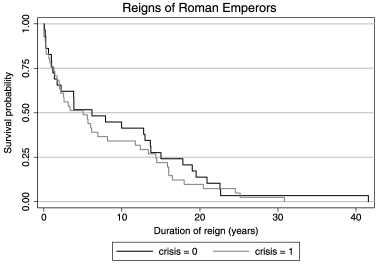
Figure 1: Empirical survival functions of durations of rule of the first 70 Roman Emperors before 235 AD (crisis${}={}$0), and after 235 AD (crisis${}={}$1).

The period 285–395 AD forms part of what is known as the Dominate, the despotic later phase of the empire. Inspection of Figure 2 suggests that the exponential hypothesis is not tenable for each separate period, so our nonparametric approach is more reasonable. The plot also suggests that the rule lengths are stochastically ordered as Dominate $\succ$ Principate $\succ$ Crisis. Applying our approach to formally test this hypothesis, we find that $T_{n}$ has a $p$-value of $0.0002$, compared with a $p$-value of 0.0017 for $S_{n}$. Under the assumption of exponential distributions, the likelihood ratio test has $p$-value less than $0.0007$.

4 Discussion

In this paper we have developed a novel empirical likelihood approach to the important problem of nonparametrically testing for the presence of stochastic ordering based on $k$ independent samples. The proposed tests are computationally efficient to implement, and could be used with massive data sets because they do not rely on the bootstrap or any other simulation technique, and they reduce to a local test for an ordering of binomial probabilities, which only requires a single sweep through the pooled data in the $k$ groups.

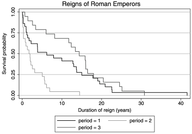
Figure 2: Empirical survival functions of durations of rule during the Principate, 27 BC–235 AD (period${}={}$1), the Crisis, 235–284 AD (period${}={}$2) and the Dominate, 284–395 AD (period${}={}$3).

Various extensions of the proposed tests are possible. In change-point problems, for example, it is of interest to test whether there is a sudden change in the distribution of a sequence of independent random variables $X_{1},\ldots,X_{n}$. Einmahl and McKeague [4] developed an EL-based change-point test for the presence of an (unknown) change-point $\tau\in\{2,\ldots,n\}$ such that

$$X_{1},\ldots,X_{\tau-1}\sim F_{1}\quad\mbox{and}\quad X_{\tau},\ldots,X_{n}\sim F_{2}.$$

They only considered the unrestricted alternative $F_{1}\neq F_{2}$, but it is also of interest to consider the ordered alternative $F_{1}\succ F_{2}$. This can be done by extending the two-sample case to allow the sample sizes to depend on an additional local parameter, namely $t\in[1/n,1)$, with $n_{1}=\lfloor nt\rfloor$ and $n_{2}=n-\lfloor nt\rfloor$. The resulting test statistic has a limiting distribution of the same form as in Theorem 2 of Einmahl and McKeague [4], involving the integral of a four-sided tied-down Wiener process $W_{0}(t,y)$, except that the integrand now includes the indicator $I(W_{0}(t,y)\geq 0)$.

Our approach also naturally extends to non-monotonic alternatives, namely to testing whether $F_{1},F_{2},\ldots,F_{k}$ are isotonic with respect to a quasi-order on $\{1,2,\ldots,k\}$. A relation $\lesssim$ on $\{1,2,\ldots,k\}$ is a quasi-order if it is reflexive and transitive (and a partial order if, in addition, it is antisymmetric). We say that $F_{1},F_{2},\ldots,F_{k}$ are isotonic with respect to $\lesssim$ if $F_{i}\succ F_{j}$ whenever $i\lesssim j$. Examples of such ordered alternatives include $F_{1}\succ F_{i}$, $i=2,\ldots,k$ (tree ordering) and $F_{1}\succ F_{2}\succ\cdots\succ F_{i_{0}}\prec F_{i_{0}+1}\prec\cdots\prec F_{k}$, where $i_{0}$ is known (umbrella ordering). The localized empirical likelihood (3) extends naturally to such ordered alternatives, the only difference being that in $\phi_{j}=E_{\mathbf{w}}(\hat{\bolds{\phi}}|\mathcal{I})_{j}$ the set $\mathcal{I}$ is now the isotonic cone corresponding to $\lesssim$. For example, in the case of tree ordering, the cone becomes $\mathcal{I}=\{\mathbf{z}\in\mathbb{R}^{k}\colon\ z_{1}\leq z_{i},i=2,\ldots,k\}$. The $\phi_{j}$ can be computed using quadratic programming or algorithms described in Robertson, Wright and Dykstra [18], one of the most general being the lower-sets algorithm. The limiting distribution of the resulting test statistic is obtained by taking $\mathcal{I}$ in (7) as the isotonic cone corresponding to $\lesssim$.

An important and challenging problem for future research in this area would be to develop EL-based tests for stochastic ordering based on censored data. EL methods are well developed for the comparison of survival functions from right-censored data, see McKeague and Zhao [13, 14], but these methods only apply to omnibus alternatives. The complication in extending the present tests to right-censored data arises because the EL ratio would then no longer have such an explicit form as in (5), and Lagrange multipliers would be involved. This extension is beyond the scope of the present paper.

5 Proofs

Proof of Theorem 1 For $0<\varepsilon<1$, let $x_{\varepsilon},y_{\varepsilon}$ be real numbers such that $F_{0}(x_{\varepsilon})=1-F_{0}(y_{\varepsilon})=\varepsilon/2$. Then decompose the test statistic as $T_{n}=T_{1n}+T_{2n}$, where

$$T_{1n}=-2\int_{x_{\varepsilon}}^{y_{\varepsilon}}\log(\mathcal{R}(x))\,\mathrm{d}F_{0}(x)\vspace*{-3pt}$$

and

$$T_{2n}=-2\int_{[x_{\varepsilon},y_{\varepsilon}]^{c}}\log(\mathcal{R}(x))\,\mathrm{d}F_{0}(x).$$

By appealing to Theorem 4.2 of Billingsley [2], note that, to complete the proof of the theorem, it suffices to show that for fixed $\varepsilon$,

$$T_{1n}\stackrel{{\scriptstyle d}}{{\rightarrow}}\int_{\varepsilon/2}^{1-\varepsilon/2}\frac{B^{2}(t)}{t(1-t)}I\bigl{(}B(t)\geq 0\bigr{)}\,\mathrm{d}t$$ (8)

as $n\to\infty$, and, for each $\delta>0$, that $\limsup_{n\to\infty}P(|T_{2n}|\geq\delta)\to 0$ as $\varepsilon\to 0$.

First consider $T_{1n}$. Using the inequality $|\log(1+y)-y+y^{2}/2|\leq|y|^{3}/3$ when $|y|\leq 1/2$, the Glivenko–Cantelli theorem and Donsker’s theorem, we have

$$\limsup_{n\to\infty}\sup_{x\in[x_{\varepsilon},y_{\varepsilon}]}\biggl{|}\log(\mathcal{R}(x))+{n\over 2}\bigl{(}\hat{F}(x)-F_{0}(x)\bigr{)}^{2}\biggl{[}\frac{1}{\hat{F}(x)}+\frac{1}{1-\hat{F}(x)}\biggr{]}I[\hat{F}(x)\leq F_{0}(x)]\biggr{|}$$

$$\quad\leq\limsup_{n\to\infty}\sup_{x\in[x_{\varepsilon},y_{\varepsilon}]}{n\over 3}|\hat{F}(x)-F_{0}(x)|^{3}\biggl{[}\frac{1}{\hat{F}(x)}+\frac{1}{1-\hat{F}(x)}\biggr{]}=0,$$

almost surely. Then, noting that $\hat{F}(x)=\hat{\Gamma}(F_{0}(x))$, where $\hat{\Gamma}$ is the empirical cdf of $V_{i}=F_{0}(X_{i})\sim U(0,1)$, $i=1,\ldots,n$, and changing variables in the integration to $t=F_{0}(x)$, it follows that

$$T_{1n} = \int_{\varepsilon/2}^{1-\varepsilon/2}n\bigl{(}\hat{\Gamma}(t)-t\bigr{)}^{2}\biggl{[}\frac{1}{\hat{\Gamma}(t)}+\frac{1}{1-\hat{\Gamma}(t)}\biggr{]}I\bigl{[}\sqrt{n}\bigl{(}\hat{\Gamma}(t)-t\bigr{)}\leq 0\bigr{]}\,\mathrm{d}t+\mathrm{o}_{p}(1)$$

$$= \int_{\varepsilon/2}^{1-\varepsilon/2}\frac{\hat{U}(t)^{2}}{t(1-t)}I[\hat{U}(t)\leq 0]\,\mathrm{d}t+\mathrm{o}_{p}(1),$$

where $\hat{U}(t)=\sqrt{n}(\hat{\Gamma}(t)-t)$ is the uniform empirical process. Note that (for any fixed $0<\varepsilon<1$) the functional

$$f\mapsto\int_{\varepsilon/2}^{1-\varepsilon/2}\frac{f(t)^{2}}{t(1-t)}I\bigl{(}f(t)\leq 0\bigr{)}\,\mathrm{d}t,\qquad f\in D[0,1],$$

is continuous when the Skorohod space $D[0,1]$ is equipped with the uniform norm. By Donsker’s theorem, $\hat{U}$ converges weakly to $B$ in $D[0,1]$, so applying the continuous mapping theorem to the leading term in (5) establishes (8).

Finally we need to verify the claim concerning $T_{2n}$. This follows immediately from a corresponding result in Einmahl and McKeague [4], who considered the test of the null hypothesis $F=F_{0}$ versus the (omnibus) alternative $F\neq F_{0}$, with the same integral-type test statistic as $T_{n}$ except that the integrand does not vanish when $\hat{F}(x)>F_{0}(x)$. This completes the proof.

Proof for Remark 1 The asymptotic distribution of $T_{n}^{*}$ can be obtained following the same steps as the proof of Theorem 1, except that the leading term in $T_{1n}$ now becomes

$$\int_{\varepsilon/2}^{1-\varepsilon/2}\frac{\hat{U}(t)^{2}}{t(1-t)}I[\hat{U}(t)\leq 0]\,\mathrm{d}\hat{\Gamma}(t)=\int_{\varepsilon/2}^{1-\varepsilon/2}V(t-)\,\mathrm{d}\hat{\Gamma}(t)+\mathrm{o}_{p}(1),$$

where

$$V(t)=\frac{\hat{U}(t)^{2}}{t(1-t)}I[\hat{U}(t)\leq 0,\varepsilon/2<t\leq 1-\varepsilon/2].$$

Note that

$$M(t)=\hat{\Gamma}(t)-\int_{0}^{t}[1-\hat{\Gamma}(s-)](1-s)^{-1}\,\mathrm{d}s$$

is a martingale wrt to the natural filtration defined by $\hat{\Gamma}$, and its predictable quadratic variation process is $\langle M\rangle(t)=n^{-1}\int_{0}^{t}[1-\hat{\Gamma}(s-)](1-s)^{-1}\,\mathrm{d}s$. Also note that $V(t-)$ is a predictable process because it is adapted and left-continuous. Write

$$\int_{\varepsilon/2}^{1-\varepsilon/2}V(t-)\,\mathrm{d}\hat{\Gamma}(t)$$

$$\quad=\int_{\varepsilon/2}^{1-\varepsilon/2}V(t-)\,\mathrm{d}M(t)+\int_{\varepsilon/2}^{1-\varepsilon/2}V(t-)[1-\hat{\Gamma}(t-)](1-t)^{-1}\,\mathrm{d}t.$$

Using a basic property of martingale integrals, the second moment of the first term above is

$$E\int_{\varepsilon/2}^{1-\varepsilon/2}V(t-)^{2}\,\mathrm{d}\langle M\rangle(t)=\mathrm{O}(1/n),$$

so this term tends in probability to zero. The second term in the above display can be handled in the same way as the main term $T_{1n}$ in the proof of Theorem 1, and has the same limit distribution.

Proof of Theorem 2 The proof is similar to the proof of Theorem 1, so we only indicate the main steps. Using the Taylor expansion of $\log(1+y)$, as before, and the (uniform) consistency of $\tilde{F}_{j}$ as an estimator of $F_{j}=F$ (see, e.g., El Barmi and Mukerjee [6], page 253), for each fixed $x$, such that $0<t=F(x)<1$, we have

$$-2\log\mathcal{R}(x) = \sum_{j=1}^{k}n_{j}\bigl{(}\tilde{F}_{j}(x)-\hat{F}(x)\bigr{)}^{2}\biggl{[}\frac{1}{\tilde{F}_{j}(x)}+\frac{1}{1-\tilde{F}_{j}(x)}\biggr{]}+\mathrm{o}_{p}(1)$$

$$= \sum_{j=1}^{k}w_{j}{[\sqrt{n}(\tilde{F}_{j}(x)-F(x))-\sqrt{n}(\hat{F}(x)-F(x))]^{2}\over F(x)(1-F(x))}+\mathrm{o}_{p}(1)$$

$$= \sum_{j=1}^{k}w_{j}\frac{(E_{\mathbf{w}}[\hat{\mathbf{U}}(t)|\mathcal{I}]_{j}-\overline{U}(t))^{2}}{t(1-t)}+\mathrm{o}_{p}(1)$$

$$\stackrel{{\scriptstyle d}}{{\rightarrow}} \sum_{j=1}^{k}w_{j}\frac{(E_{\mathbf{w}}[\mathbf{B}(t)|\mathcal{I}]_{j}-\overline{B}(t))^{2}}{t(1-t)},$$

where $\hat{\mathbf{U}}=(\hat{U}_{1}/\sqrt{w_{1}},\hat{U}_{2}/\sqrt{w_{2}},\ldots,\hat{U}_{k}/\sqrt{w_{k}})^{T}$, $\hat{U}_{j}(t)=\sqrt{n_{j}}(\hat{F}_{j}(x)-F(x))$ are independent uniform empirical processes, and $\overline{U}=\sum_{j=1}^{k}\sqrt{w}_{j}\hat{U}_{j}.$ Donsker’s theorem and the continuous mapping theorem have been used as before, but we have also used the fact that $E_{\bf w}(\cdot|\mathcal{I})$ is a continuous function on $\mathbb{R}^{k}$.

References

- [1] {barticle}[mr] \bauthor\bsnmBaringhaus, \bfnmLudwig\binitsL. &\bauthor\bsnmGrübel, \bfnmRudolf\binitsR. (\byear2009). \btitleNonparametric two-sample tests for increasing convex order. \bjournalBernoulli \bvolume15 \bpages99–123. \biddoi=10.3150/08-BEJ151, issn=1350-7265, mr=2546800 \bptokimsref \endbibitem
- [2] {bbook}[mr] \bauthor\bsnmBillingsley, \bfnmPatrick\binitsP. (\byear1968). \btitleConvergence of Probability Measures. \baddressNew York: \bpublisherWiley. \bidmr=0233396 \bptokimsref \endbibitem
- [3] {barticle}[mr] \bauthor\bsnmDykstra, \bfnmRichard L.\binitsR.L., \bauthor\bsnmMadsen, \bfnmRichard W.\binitsR.W. &\bauthor\bsnmFairbanks, \bfnmKenneth\binitsK. (\byear1983). \btitleA nonparametric likelihood ratio test. \bjournalJ. Statist. Comput. Simulation \bvolume18 \bpages247–264. \biddoi=10.1080/00949658308810702, issn=0094-9655, mr=0746554 \bptokimsref \endbibitem
- [4] {barticle}[mr] \bauthor\bsnmEinmahl, \bfnmJohn H. J.\binitsJ.H.J. &\bauthor\bsnmMcKeague, \bfnmIan W.\binitsI.W. (\byear2003). \btitleEmpirical likelihood based hypothesis testing. \bjournalBernoulli \bvolume9 \bpages267–290. \biddoi=10.3150/bj/1068128978, issn=1350-7265, mr=1997030 \bptokimsref \endbibitem
- [5] {barticle}[mr] \bauthor\bsnmEl Barmi, \bfnmHammou\binitsH. &\bauthor\bsnmJohnson, \bfnmMatthew\binitsM. (\byear2006). \btitleA unified approach to testing for and against a set of linear inequality constraints in the product multinomial setting. \bjournalJ. Multivariate Anal. \bvolume97 \bpages1894–1912. \biddoi=10.1016/j.jmva.2005.06.006, issn=0047-259X, mr=2298895 \bptokimsref \endbibitem
- [6] {barticle}[mr] \bauthor\bsnmEl Barmi, \bfnmHammou\binitsH. &\bauthor\bsnmMukerjee, \bfnmHari\binitsH. (\byear2005). \btitleInferences under a stochastic ordering constraint: The -sample case. \bjournalJ. Amer. Statist. Assoc. \bvolume100 \bpages252–261. \biddoi=10.1198/016214504000000764, issn=0162-1459, mr=2156835 \bptokimsref \endbibitem
- [7] {barticle}[mr] \bauthor\bsnmFranck, \bfnmWallace E.\binitsW.E. (\byear1984). \btitleA likelihood ratio test for stochastic ordering. \bjournalJ. Amer. Statist. Assoc. \bvolume79 \bpages686–691. \bidissn=0162-1459, mr=0763587 \bptokimsref \endbibitem
- [8] {barticle}[mr] \bauthor\bsnmHogg, \bfnmRobert V.\binitsR.V. (\byear1962). \btitleIterated tests of the equality of several distributions. \bjournalJ. Amer. Statist. Assoc. \bvolume57 \bpages579–585. \bidissn=0162-1459, mr=0159373 \bptokimsref \endbibitem
- [9] {barticle}[mr] \bauthor\bsnmKhmaladze, \bfnmEstate\binitsE., \bauthor\bsnmBrownrigg, \bfnmRay\binitsR. &\bauthor\bsnmHaywood, \bfnmJohn\binitsJ. (\byear2007). \btitleBrittle power: On Roman Emperors and exponential lengths of rule. \bjournalStatist. Probab. Lett. \bvolume77 \bpages1248–1257. \biddoi=10.1016/j.spl.2007.03.009, issn=0167-7152, mr=2392795 \bptokimsref \endbibitem
- [10] {barticle}[mr] \bauthor\bsnmLee, \bfnmYoung Jack\binitsY.J. &\bauthor\bsnmWolfe, \bfnmDouglas A.\binitsD.A. (\byear1976). \btitleA distribution-free test for stochastic ordering. \bjournalJ. Amer. Statist. Assoc. \bvolume71 \bpages722–727. \bidissn=0162-1459, mr=0443208 \bptokimsref \endbibitem
- [11] {barticle}[mr] \bauthor\bsnmLehmann, \bfnmE. L.\binitsE.L. (\byear1955). \btitleOrdered families of distributions. \bjournalAnn. Math. Statist. \bvolume26 \bpages399–419. \bidissn=0003-4851, mr=0071684 \bptokimsref \endbibitem
- [12] {barticle}[mr] \bauthor\bsnmMau, \bfnmJochen\binitsJ. (\byear1988). \btitleA generalization of a nonparametric test for stochastically ordered distributions to censored survival data. \bjournalJ. Roy. Statist. Soc. Ser. B \bvolume50 \bpages403–412. \bidissn=0035-9246, mr=0970976 \bptokimsref \endbibitem
- [13] {barticle}[mr] \bauthor\bsnmMcKeague, \bfnmIan W.\binitsI.W. &\bauthor\bsnmZhao, \bfnmYichuan\binitsY. (\byear2002). \btitleSimultaneous confidence bands for ratios of survival functions via empirical likelihood. \bjournalStatist. Probab. Lett. \bvolume60 \bpages405–415. \biddoi=10.1016/S0167-7152(02)00309-7, issn=0167-7152, mr=1947180 \bptokimsref \endbibitem
- [14] {barticle}[mr] \bauthor\bsnmMcKeague, \bfnmIan W.\binitsI.W. &\bauthor\bsnmZhao, \bfnmYichuan\binitsY. (\byear2005). \btitleComparing distribution functions via empirical likelihood. \bjournalInt. J. Biostat. \bvolume1 \bpagesArt. 5, 20 pp. (electronic). \bidissn=1557-4679, mr=2232230 \bptokimsref \endbibitem
- [15] {barticle}[mr] \bauthor\bsnmOwen, \bfnmArt\binitsA. (\byear1990). \btitleEmpirical likelihood ratio confidence regions. \bjournalAnn. Statist. \bvolume18 \bpages90–120. \biddoi=10.1214/aos/1176347494, issn=0090-5364, mr=1041387 \bptokimsref \endbibitem
- [16] {barticle}[mr] \bauthor\bsnmOwen, \bfnmArt B.\binitsA.B. (\byear1988). \btitleEmpirical likelihood ratio confidence intervals for a single functional. \bjournalBiometrika \bvolume75 \bpages237–249. \biddoi=10.1093/biomet/75.2.237, issn=0006-3444, mr=0946049 \bptokimsref \endbibitem
- [17] {barticle}[mr] \bauthor\bsnmRobertson, \bfnmTim\binitsT. &\bauthor\bsnmWright, \bfnmF. T.\binitsF.T. (\byear1981). \btitleLikelihood ratio tests for and against a stochastic ordering between multinomial populations. \bjournalAnn. Statist. \bvolume9 \bpages1248–1257. \bidissn=0090-5364, mr=0630107 \bptokimsref \endbibitem
- [18] {bbook}[mr] \bauthor\bsnmRobertson, \bfnmTim\binitsT., \bauthor\bsnmWright, \bfnmF. T.\binitsF.T. &\bauthor\bsnmDykstra, \bfnmR. L.\binitsR.L. (\byear1988). \btitleOrder Restricted Statistical Inference. \bseriesWiley Series in Probability and Mathematical Statistics: Probability and Mathematical Statistics. \baddressChichester: \bpublisherWiley. \bidmr=0961262 \bptokimsref \endbibitem
- [19] {bbook}[auto:STB—2011/12/02—17:21:01] \bauthor\bsnmShaked, \bfnmM.\binitsM. &\bauthor\bsnmShanthikumar, \bfnmG. J.\binitsG.J. (\byear2006). \btitleStochastic Orders. \baddressNew York: \bpublisherSpringer. \bptokimsref \endbibitem
- [20] {bbook}[mr] \bauthor\bsnmSilvapulle, \bfnmMervyn J.\binitsM.J. &\bauthor\bsnmSen, \bfnmPranab K.\binitsP.K. (\byear2005). \btitleConstrained Statistical Inference: Inequality, Order, and Shape Restrictions. \bseriesWiley Series in Probability and Statistics. \baddressHoboken, NJ: \bpublisherWiley-Interscience. \bidmr=2099529 \bptokimsref \endbibitem
- [21] {barticle}[mr] \bauthor\bsnmWang, \bfnmYazhen\binitsY. (\byear1996). \btitleA likelihood ratio test against stochastic ordering in several populations. \bjournalJ. Amer. Statist. Assoc. \bvolume91 \bpages1676–1683. \bidissn=0162-1459, mr=1439109 \bptokimsref \endbibitem