Abstract

This paper is concerned with the direct and inverse acoustic or electromagnetic scattering problems by a locally perturbed, perfectly reflecting, infinite plane (which is called a locally rough surface in this paper). We propose a novel integral equation formulation for the direct scattering problem which is defined on a bounded curve (consisting of a bounded part of the infinite plane containing the local perturbation and the lower part of a circle) with two corners. This novel integral equation can be solved efficiently by using the Nyström method with a graded mesh introduced previously by Kress and is capable of dealing with large wavenumber cases. For the inverse problem, we propose a Newton iteration method to reconstruct the local perturbation of the plane from multiple frequency far-field data, based on the novel integral equation formulation. Numerical examples are carried out to demonstrate that our reconstruction method is stable and accurate even for the case of multiple-scale profiles.

Keywords: Integral equation, locally rough surface, inverse scattering problem, far field pattern, perfectly reflecting surface, Newton iteration.

1 Introduction

Consider problems of scattering of plane acoustic or electromagnetic waves by a locally perturbed, perfectly reflecting, infinite plane (which is called a locally rough surface). Such problems occur in many applications such as radar, remote sensing, geophysics, medical imaging and nondestructive testing (see, e.g. [2, 4, 7, 8, 19]).

In this paper we restrict the discussion to the two-dimensional case by assuming that the local perturbation is invariant in the $x_{3}$ direction. We assume throughout that the incident wave is time-harmonic ($e^{-i\omega t}$ time dependence), so that the total wave field $u$ satisfies the Helmholtz equation

$$\Delta u+k^{2}u=0\quad\mbox{in}\;\;D_{+}.$$ (1.1)

Here, $D_{+}:=\{(x_{1},x_{2})\;|\;x_{2}>h_{\Gamma}(x_{1}),x_{1}\in{\mathbb{R}}\}$ represents a homogeneous medium above the locally rough surface denoted by $\Gamma:=\partial D_{+}=\{(x_{1},x_{2})\;|\;x_{2}=h_{\Gamma}(x_{1}),x_{1}\in{\mathbb{R}}\}$ with some smooth function $h_{\Gamma}\in C^{2}({\mathbb{R}})$ having a compact support in ${\mathbb{R}}$, $k=\omega/c>0$ is the wave number, $\omega$ and $c$ are the frequency and speed of the wave in $D_{+}$, respectively. Throughout, we will assume that the incident field $u^{i}$ is the plane wave

$$u^{i}(x)=\exp({ikd\cdot x}),$$

where $d=(\sin\theta,-\cos\theta)\in S_{-}$ is the incident direction, $\theta$ is the angle of incidence, measured from the $x_{2}-$axis with $-\pi/2<\theta<\pi/2,$ and $S_{-}:=\{x=(x_{1},x_{2})\;|\;|x|=1,x_{2}<0\}$ is the lower part of the unit circle $S=\{x\in{\mathbb{R}}^{2}\;|\;|x|=1\}$. We further assume that the total field $u(x)=u^{i}(x)+u^{r}(x)+u^{s}(x)$ vanishes on the surface $\Gamma$:

$$u(x)=u^{i}(x)+u^{r}(x)+u^{s}(x)=0\qquad\mbox{on}\;\;\Gamma,$$ (1.2)

where $u^{r}$ is the reflected wave by the infinite plane $x_{2}=0$:

$$u^{r}(x)=-\exp(ik[x_{1}\sin\theta+x_{2}\cos\theta])$$

and $u^{s}$ is the unknown scattered wave to be determined which is required to satisfy the Sommerfeld radiation condition

$$\lim_{r\to\infty}r^{\frac{1}{2}}\left(\frac{\partial u^{s}}{\partial r}-iku^{s}\right)=0,\quad r=|x|,\quad x\in D_{+}.$$ (1.3)

This problem models scattering of electromagnetic plane waves by a locally perturbed, perfectly conducting, infinite plane in the TE polarization case; it also models acoustic scattering by a one-dimensional sound-soft surface. Figure 1 presents the problem geometry.

The well-posedness of the scattering problem (1.1)-(1.3) has been studied by using the variational method with a Dirichlet-to-Neumann (DtN) map in [4] or the integral equation method in [30]. In particular, it was proved in [30] that $u^{s}$ has the following asymptotic behavior at infinity:

$$u^{s}(x)=\frac{e^{ik|x|}}{\sqrt{|x|}}\left(u^{\infty}(\hat{x};d)+O\Big{(}\frac{1}{|x|}\Big{)}\right),\qquad|x|\to\infty$$

uniformly for all observation directions $\hat{x}\in S_{+}$ with $S_{+}:=\{x=(x_{1},x_{2})\;|\;|x|=1,x_{2}>0\}$ the upper part of the unit circle $S$, where $u^{\infty}(\hat{x};d)$ is called the far field pattern of the scattered field $u^{s}$, depending on the observation direction $\hat{x}$ and the incident direction $d\in S_{-}$. The integral equation formulation obtained in [30] is of the second kind with a compact integral operator defined on the local perturbation part of the infinite plane. However, it is not suitable for numerical computation since it also involves an infinite integral over the unbounded, unperturbed part of the infinite plane. In [4], the scattering problem (1.1)-(1.3) is reformulated as an equivalent boundary value problem in a bounded domain with a DtN map on the part in $D_{+}$ of a large circle enclosing the local perturbation of the plane. This equivalent boundary value problem with a non-local boundary condition is then solved numerically by using the integral equation approach. However, the integral equation thus obtained involves a non-local DtN map on the semi-circle which needs to be truncated in numerical computations.

In this paper, we propose a novel integral equation formulation for the scattering problem (1.1)-(1.3), which is defined on a bounded curve (consisting of a bounded part of the infinite plane containing the local perturbation and the lower part of a circle) with two corners. Compared with [4] and [30], our integral equation formulation does not involve any infinite integral or a DtN map and therefore leads to fast numerical solution of the scattering problem including the large wavenumber cases. In fact, our integral equation can be solved efficiently by using the Nyström method with a graded mesh at the two corners introduced previously by Kress [24] (see Section 3 below). Furthermore, we are also interested in the inverse problem of determining the locally rough surface from the far field pattern $u^{\infty}(\hat{x},d)$ for all $\hat{x}\in S_{+},\;d\in S_{-}$. A Newton iteration method is presented to reconstruct the locally rough surface from multi-frequency far field data, and our novel integral equation is applied to solve the direct scattering problem in each iteration. From the numerical examples it is seen that multi-frequency data are necessary in order to get a stable and accurate reconstruction of the locally rough surface.

The mathematical and computational aspects of the scattering problem (1.1)-(1.3) have been studied extensively in the case when the local perturbation is below the infinite plane which is called the cavity problem (see, e.g. [1, 2, 6] and the references quoted there) and for the case of non-local perturbations which is called the rough surface scattering (see, e.g. [8, 9, 10, 11, 12, 13, 31]).

There are many works concerning numerical solutions of the inverse problem of reconstructing the rough surfaces from the scattered field data. For example, a Newton method was proposed in [27] to reconstruct a local rough surface from the far-field pattern under the condition that the local perturbation is both star-like and over the infinite plane. An optimization method was introduced in [3] to recover a mild, local rough surface from the scattered field measured on a straight line within one wavelength above the local rough surface, under the assumption that the local perturbation is over the infinite plane. In [4], a continuation approach over the wave frequency was developed for reconstructing a general, local rough surface from the scattered field measured on an upper half-circle enclosing the local perturbation, based on the choice of the descent vector field. The reconstruction obtained in [4] is stable and accurate due to the use of multi-frequency near-field data (see also [5]). It should be pointed out that the reconstruction algorithm developed in [4] does not work with multi-frequency far-field data. Note that our novel integral equation formulation can also be used to develop a similar Newton inversion algorithm with multiple frequency near-field data. For the numerical recovery of non-local rough surfaces we refer to [7, 14, 15, 19, 20]. For the inverse cavity problem, the reader is referred to [2, 21, 28].

This paper is organized as follows. In Section 2, a novel integral equation formulation is proposed to solve the direct scattering problem. Section 3 is devoted to the numerical solution of the novel integral equation. In Section 4, it is proved that the local rough surface can be uniquely determined by the far-field pattern corresponding to a countably infinite number of incident plane waves. The Frechet differentiability is also shown of the far-field operator which maps the surface profile function $h_{\Gamma}$ to the corresponding far field pattern $u^{\infty}_{k}(\hat{x},d)$. The Newton method with multi-frequency far-field data is given in Section 5, based on the novel integral equation solver in Section 3. In Section 6, numerical examples are carried out to demonstrate that our reconstruction algorithm is stable and accurate even for the case of multiple-scale profiles, which is similar to the inversion algorithm with multi-frequency near-field data developed in [4].

2 A novel integral equation formulation for the direct problem

Let $f=-(u^{i}+u^{r}).$ Then $f$ is continuous on $\Gamma$ and $f=0$ on $\Gamma_{0}:=\{(x_{1},x_{2})\in\Gamma\;|\;x_{2}=0\}$, that is, $f$ has a compact support on $\Gamma$. The scattering problem (1.1)-(1.3) can be reformulated as the Dirichlet problem (DP) in the following way:

Find $u^{s}\in C^{2}(D_{+})\cap C(\overline{D_{+}})$ satisfying the Helmholtz equation (1.1) in $D_{+},$ the Sommerfeld radiation condition (1.3) and the Dirichlet boundary condition:

$$u^{s}=f\qquad\mbox{on}\quad\Gamma.$$ (2.1)

The following uniqueness result has been proved in [30, Theorem 3.1] for the above Dirichlet problem (DP).

Theorem 2.1.

The problem (DP) has at most one solution in $C^{2}(D_{+})\cap C(\overline{D}_{+})$.

The existence of solutions to the problem (DP) has also been studied in [30] using an integral equation method. However, the integral equation obtained in [30] involves an infinite integral which yields difficulties in numerical computation. In this section, we propose a new integral equation to avoid this problem. To this end, we introduce the following notations. Let $B_{R}\coloneqq\{x=(x_{1},x_{2})\;|\;|x|<R\}$ be a circle with $R>0$ large enough so that the local perturbation $\Gamma_{p}:=\Gamma\backslash\Gamma_{0}=\{(x_{1},h_{\Gamma}(x_{1}))\;|\;x_{1}\in\textrm{supp}(h_{\Gamma})\}\subset B_{R}$. Then $\Gamma_{R}\coloneqq\Gamma\cap B_{R}$ represents the part of $\Gamma$ containing the local perturbation $\Gamma_{p}$ of the infinite plane. Denote by $x_{A}:=(-R,0),x_{B}:=(R,0)$ the endpoints of $\Gamma_{R}$. Write $\mathbb{R}^{2}_{\pm}\coloneqq\{(x_{1},x_{2})\in{\mathbb{R}}^{2}\;|\;x_{2}\gtrless 0\}$, $D^{\pm}_{R}\coloneqq B_{R}\cap D_{\pm}$ and $\partial B^{\pm}_{R}\coloneqq\partial B_{R}\cap D_{\pm}$, where $D_{-}:=\{(x_{1},x_{2})\;|\;x_{2}<h_{\Gamma}(x_{1}),x_{1}\in{\mathbb{R}}\}.$ See Figure 1.

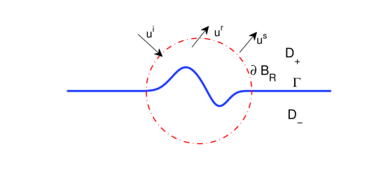
Figure 1: The scattering problem from a locally rough surface

For $\varphi\in C(\partial D_{R}^{-})$ define $\mathcal{S}_{k}$ and $\mathcal{D}_{k}$ to be the single- and double-layer potentials:

$$(\mathcal{S}_{k}\varphi)(x) := \int_{\partial D^{-}_{R}}\Phi_{k}(x,y)\varphi(y)ds(y),\quad x\in\mathbb{R}^{2}\backslash\partial D^{-}_{R}$$

$$(\mathcal{D}_{k}\varphi)(x) := \int_{\partial D^{-}_{R}}\frac{\partial\Phi_{k}(x,y)}{\partial\nu(y)}\varphi(y)ds(y),\quad x\in\mathbb{R}^{2}\backslash\partial D^{-}_{R}$$

and define $S_{k},S_{k}^{re},K_{k},K_{k}^{re}$ to be the boundary integral operators of the following form:

$$(S_{k}\varphi)(x) := \int_{\partial D^{-}_{R}}\Phi_{k}(x,y)\varphi(y)ds(y),\quad x\in\partial D^{-}_{R}$$

$$(S_{k}^{re}\varphi)(x) := \left\{\begin{array}[]{l}\displaystyle\int_{\partial D^{-}_{R}}\Phi_{k}(x,y)\varphi(y)ds(y),\quad x\in\Gamma_{R}\\ \displaystyle\int_{\partial D^{-}_{R}}\Phi_{k}(x^{re},y)\varphi(y)ds(y),\quad x\in\partial B^{-}_{R}\cup\{x_{A},x_{B}\}\end{array}\right.$$

$$(K_{k}\varphi)(x) := \int_{\partial D^{-}_{R}}\frac{\partial\Phi_{k}(x,y)}{\partial\nu(y)}\varphi(y)ds(y),\quad x\in\partial D^{-}_{R}$$

$$(K_{k}^{re}\varphi)(x) := \left\{\begin{array}[]{l}\displaystyle\int_{\partial D^{-}_{R}}\frac{\partial\Phi_{k}(x,y)}{\partial\nu(y)}\varphi(y)ds(y),\quad x\in\Gamma_{R}\\ \displaystyle\int_{\partial D^{-}_{R}}\frac{\partial\Phi_{k}(x^{re},y)}{\partial\nu(y)}\varphi(y)ds(y),\quad x\in\partial B^{-}_{R}\cup\{x_{A},x_{B}\}\end{array}\right.$$

where $x^{re}=(x_{1},-x_{2})$ is the reflection of $x=(x_{1},x_{2})$ about the $x_{1}$-axis, $\Phi_{k}(x,y)$ is the fundamental solution of the Helmholtz equation $\Delta w+k^{2}w=0$ with the wavenumber $k$, and $\nu$ is the unit outward normal on $\partial D^{-}_{R}$. Note that $\Phi_{0}(x,y)=-{1}/({2\pi})\ln{|x-y|}$ is the fundamental solution of the Laplace equation.

Remark 2.2.

Let $\varphi\in C(\partial D^{-}_{R})$. From [22, Theorem 15.8b] it follows that the single-layer potential $\mathcal{S}_{k}\varphi$ is continuous throughout ${\mathbb{R}}^{2}$. In addition, from [26, Section 6.5] we know that the double-layer potential $\mathcal{D}_{0}\varphi$ can be continuously extended from ${\mathbb{R}}^{2}\backslash\overline{D}^{-}_{R}$ to ${\mathbb{R}}^{2}\backslash D^{-}_{R}$ with the limiting value

$$(\mathcal{D}_{0}\varphi)_{+}(x)=\left\{\begin{array}[]{ll}\displaystyle(K_{0}\varphi)(x)+\frac{1}{2}\varphi(x)&\mbox{for}\;x\in\partial D^{-}_{R}\backslash\{x_{A},x_{B}\}\\ \displaystyle(K_{0}\varphi)(x)+\frac{\gamma(x)}{2\pi}\varphi(x)&\mbox{for}\;x\in\{x_{A},x_{B}\}\end{array}\right.$$

where $\gamma(x)$ is the interior angle at the corner $x\in\{x_{A},x_{B}\}$. It remains valid for $\mathcal{D}_{k}\varphi$ with $k>0$ since the kernel of $\mathcal{D}_{k}-\mathcal{D}_{0}$ is weakly singular which yields that $(\mathcal{D}_{k}-\mathcal{D}_{0})\varphi$ is continuous throughout ${\mathbb{R}}^{2}$. Thus from the jump relations, $S_{k}$, $S_{k}^{re}$, $\widetilde{K}_{k}$ and $\widetilde{K}^{re}_{k}$ are bounded in $C(\partial D^{-}_{R})$, where $\widetilde{K}_{k}$ and $\widetilde{K}^{re}_{k}$ are given by

$$(\widetilde{K}_{k}\varphi)(x) := \left\{\begin{array}[]{ll}\displaystyle(K_{k}\varphi)(x)&\mbox{for}\;x\in\partial D^{-}_{R}\backslash\{x_{A},x_{B}\}\\ \displaystyle(K_{k}\varphi)(x)+\left(\frac{\gamma(x)}{2\pi}-\frac{1}{2}\right)\varphi(x)&\mbox{for}\;x\in\{x_{A},x_{B}\}\end{array}\right.$$

$$(\widetilde{K}^{re}_{k}\varphi)(x) := \left\{\begin{array}[]{ll}\displaystyle(K^{re}_{k}\varphi)(x)&\mbox{for}\;x\in\partial D^{-}_{R}\backslash\{x_{A},x_{B}\}\\ \displaystyle(K^{re}_{k}\varphi)(x)+\left(\frac{\gamma(x)}{2\pi}-\frac{1}{2}\right)\varphi(x)&\mbox{for}\;x\in\{x_{A},x_{B}\}\end{array}\right.$$

In particular, $S_{k}-S_{0}$, $S^{re}_{k}-S^{re}_{0}$, $K_{k}-K_{0}$ and $K^{re}_{k}-K^{re}_{0}$ are bounded in $C(\partial D^{-}_{R})$.

Let $u^{s}$ be the solution of the problem (DP). Then we can extend $u^{s}(x)$ into ${\mathbb{R}}^{2}_{-}\backslash\overline{B}_{R}$ by reflection, which is denoted again by $u^{s}(x)$, such that $u^{s}(x)=-u^{s}(x^{re})$ in ${\mathbb{R}}^{2}_{-}\backslash\overline{B}_{R}$. By a regularity argument (see [16, page 88] or [30, Theorem 3.1]) and the reflection principle, we know that $u^{s}\in C^{2}({\mathbb{R}}^{2}\backslash\overline{D}_{R}^{-})\cap C({\mathbb{R}}^{2}\backslash D_{R}^{-})$ and satisfies the Helmholtz equation (1.1) in ${\mathbb{R}}^{2}\backslash\overline{D}_{R}^{-}$. Following the idea in [17], we seek the solution $u^{s}$ in the form

$$u^{s}(x)=(\mathcal{D}_{k}\varphi)(x)-i\eta(\mathcal{S}_{k}\varphi)(x),\quad\varphi\in C(\partial D_{R}^{-}),\quad x\in{\mathbb{R}}^{2}\backslash\partial D_{R}^{-}$$ (2.7)

where $\eta\neq 0$ is a real coupling parameter. Let $\psi^{re}$ be a continuous mapping from $\partial D_{R}^{-}$ to $\partial D_{R}^{+}$ such that

$$\psi^{re}(x)=\left\{\begin{array}[]{ll}x,&x\in\Gamma_{R}\\ x^{re},&x\in\partial B_{R}^{-}\cup\{x_{A},x_{B}\}\end{array}\right.$$

Since $u^{s}(x)+u^{s}(\psi^{re}(x))=-2\big{[}u^{i}(x)+u^{r}(x)\big{]}$ on $\Gamma_{R}$ and $u^{s}(x)+u^{s}(\psi^{re}(x))=0$ on $\partial B_{R}^{-}\cup\{x_{A},x_{B}\}$, and by the jump relations of the layer potentials, we obtain the boundary integral equation $P\varphi(x)=g(x)$, where

$$P\varphi\coloneqq\left\{\begin{array}[]{ll}\displaystyle\varphi+\left(K_{k}\varphi-i\eta S_{k}\varphi\right)+\left(K^{re}_{k}\varphi-i\eta S_{k}^{re}\varphi\right),&x\in\Gamma_{R}\\ \displaystyle\frac{1}{2}\varphi+\left(K_{k}\varphi-i\eta S_{k}\varphi\right)+\left(K^{re}_{k}\varphi-i\eta S^{re}_{k}\varphi\right),&x\in\partial B_{R}^{-}\cup\{x_{A},x_{B}\}\end{array}\right.$$ (2.11)

and

$$g(x):=\left\{\begin{array}[]{ll}-2\big{(}u^{i}(x)+u^{r}(x)\big{)},&x\in\Gamma_{R}\\ 0,&x\in\partial B_{R}^{-}\cup\{x_{A},x_{B}\}\end{array}\right.$$ (2.14)

Here, we have used the fact that the interior angles $\gamma(x)$ at the corners $x_{A},x_{B}$ are both $\pi/2$. Note that $g\in C(\partial D_{R}^{-})$. Further, from Remark 2.2 and the continuity of $\psi^{re}$ it follows that $P$ is a bounded linear operator in $C(\partial D_{R}^{-})$.

Conversely, we have the following result.

Lemma 2.3.

Assume that $u^{s}$ is of the form (2.7) with $\varphi\in C(\partial D_{R}^{-})$ which satisfies the integral equation $P\varphi=g$ with $P$, $g$ defined in (2.11), (2.14), respectively. Then $u^{s}\in C^{2}(D_{+})\cap C(\overline{D}_{+})$ and solves the problem (DP).

Proof.

Since $\varphi\in C(\partial D_{R}^{-})$, it follows from Remark 2.2 that $u^{s}\in C^{2}({\mathbb{R}}^{2}\backslash\overline{D}_{R}^{-})\cap C({\mathbb{R}}^{2}\backslash D_{R}^{-})$ and satisfies the Helmholtz equation (1.1) in ${\mathbb{R}}^{2}\backslash\overline{D}_{R}^{-}$. In addition, $P\varphi=g$ implies that $u^{s}(x)+u^{s}(x^{re})=0$ on $\partial B_{R}^{-}\cup\{x_{A},x_{B}\}$ and $u^{s}(x)=-\big{(}u^{i}(x)+u^{r}(x)\big{)}$ on $\Gamma_{R}$.

Let $\tilde{u}^{s}(x)=-u^{s}(x^{re})$ in ${\mathbb{R}}^{2}\backslash B_{R}$. Then $\tilde{u}^{s}$ satisfies the Helmholtz equation (1.1) in ${\mathbb{R}}^{2}\backslash\overline{B}_{R}$ and $\tilde{u}^{s}(x)=u^{s}(x)$ on $\partial B_{R}$. Moreover, the uniqueness of the exterior Dirichlet problem (see, e.g. [17, Chapter 3]) implies that $\tilde{u}^{s}=u^{s}$ in ${\mathbb{R}}^{2}\backslash B_{R}$. In particular, $u^{s}(x)=0$ on $\Gamma\backslash\Gamma_{R}$ which yields that $u^{s}(x)=-(u^{i}+u^{r})$ on $\Gamma$. The proof is thus completed. ∎

We now prove the unique solvability of the integral equation $P\varphi=g$.

Theorem 2.4.

The integral equation $P\varphi=g$ has a unique solution $\varphi\in C(\partial D_{R}^{-})$ satisfying the estimate

$$||\varphi||_{C(\partial D_{R}^{-})}\leq C||u^{i}+u^{r}||_{C(\Gamma)}$$ (2.15)

Proof.

We need to deal with the corners. Following the idea in [17], we introduce the following boundary integral operators: for $z=x_{A},x_{B}$

$$K_{0,z}\varphi(x) \coloneqq \int_{\partial D_{R}^{-}}\frac{\partial\Phi_{0}(x,y)}{\partial\nu(y)}\varphi(z)ds(y),\quad x\in\partial D_{R}^{-}$$

$$K^{re}_{0,z}\varphi(x) \coloneqq \left\{\begin{array}[]{l}\displaystyle\int_{\partial D_{R}^{-}}\frac{\partial\Phi_{0}(x,y)}{\partial\nu(y)}\varphi(z)ds(y),\quad x\in\Gamma_{R}\\ \displaystyle\int_{\partial D_{R}^{-}}\frac{\partial\Phi_{0}(x^{re},y)}{\partial\nu(y)}\varphi(z)ds(y),\quad x\in\partial B_{R}^{-}\cup\{x_{A},x_{B}\}\end{array}\right.$$

For $z=x_{A},x_{B}$ define $B_{\varepsilon}(z)\coloneqq\{x\in{\mathbb{R}}^{2}\;|\;|x-z|<\varepsilon\}$ with radius $\varepsilon$ small enough such that $B_{\varepsilon}(z)\cap(\Gamma\backslash\Gamma_{0})=\emptyset$. Choose a cut-off function $\chi\in C^{\infty}_{0}({\mathbb{R}}^{2})$ satisfying that $0\leq\chi\leq 1$, $\chi(x)=\chi(x^{re})$, $\chi=1$ in $B_{\varepsilon}(x_{A})$ and $\chi=0$ in $B_{\varepsilon}(x_{B})$. Since $K_{0,z}\varphi$ vanishes in ${\mathbb{R}}^{2}\backslash\overline{D}_{R}^{-}$ for $z=x_{A},x_{B}$, we can rewrite (2.7) in the following form:

$$u^{s}(x) = \chi(x)\left[\int_{\partial D_{R}^{-}}\left(\frac{\partial\Phi_{k}(x,y)}{\partial\nu(y)}-i\eta\Phi_{k}(x,y)\right)\varphi(y)ds(y)-\int_{\partial D_{R}^{-}}\frac{\partial\Phi_{0}(x,y)}{\partial\nu(y)}\varphi(x_{A})ds(y)\right]$$

$$+[1-\chi(x)]\left[\int_{\partial D_{R}^{-}}\left(\frac{\partial\Phi_{k}(x,y)}{\partial\nu(y)}-i\eta\Phi_{k}(x,y)\right)\varphi(y)ds(y)\right.$$

$$\qquad\qquad\left.-\int_{\partial D_{R}^{-}}\frac{\partial\Phi_{0}(x,y)}{\partial\nu(y)}\varphi(x_{B})ds(y)\right],\quad x\in{\mathbb{R}}^{2}\backslash\overline{D}_{R}^{-}$$

Accordingly, using the jump relations of the layer potentials and the fact that $\chi(x)=\chi(x^{re})$, we rewrite $P\varphi$, defined in (2.11), as $P\varphi=I_{\chi}\varphi+A\varphi+B\varphi$, where

$$(I_{\chi}\varphi)(x) \coloneqq \left\{\begin{array}[]{ll}\displaystyle\varphi(x),&x\in\Gamma_{R}\\ \displaystyle(1/2)[\varphi(x)+\chi\varphi(x_{A})+(1-\chi)\varphi(x_{B})],&x\in\partial B_{R}^{-}\cup\{x_{A},x_{B}\}\end{array}\right.$$

$$(A\varphi)(x) \coloneqq -\chi(x)\varphi(x_{A})-[1-\chi(x)]\varphi(x_{B})$$

$$(B\varphi)(x) \coloneqq \chi(x)\left(K_{k}\varphi-i\eta S_{k}\varphi-K_{0,x_{A}}\varphi\right)(x)+[1-\chi(x)]\left(K_{k}\varphi-i\eta S_{k}\varphi-K_{0,x_{B}}\varphi\right)(x)$$

$$\qquad+\chi(x)\left(K^{re}_{k}\varphi-i\eta S^{re}_{k}\varphi-K^{re}_{0,x_{A}}\varphi\right)(x)+[1-\chi(x)]\left(K^{re}_{k}\varphi-i\eta S^{re}_{k}\varphi-K^{re}_{0,x_{B}}\varphi\right)(x)$$

Here, $I_{\chi},A$ are bounded in $C(\partial D_{R}^{-})$. From Remark 2.2, $B$ is also bounded in $C(\partial D_{R}^{-})$.

Step 1. We show that $P$ is a Fredholm operator of index zero.

Let

$$(M_{0}\varphi)(x) \coloneqq \chi(x)\left(K_{0}\varphi-K_{0,x_{A}}\varphi\right)(x)+[1-\chi(x)]\left(K_{0}\varphi-K_{0,x_{B}}\varphi\right)(x)$$

$$+\chi(x)\left(K^{re}_{0}\varphi-K^{re}_{0,x_{A}}\varphi\right)(x)+[1-\chi(x)]\left(K^{re}_{0}\varphi-K^{re}_{0,x_{B}}\varphi\right)(x)$$

From Remark 2.2 it is easy to see that $M_{0}$ is bounded in $C(\partial D_{R}^{-})$. Since the integral operator $B-M_{0}$ has a weakly singular kernel and $\psi^{re}$ is a continuous mapping, the operator $B-M_{0}$ is compact in $C(\partial D_{R}^{-})$. Thus, $P-(I_{\chi}+M_{0})=A+B-M_{0}$ is compact in $C(\partial D_{R}^{-})$.

Moreover, for $z=x_{A},x_{B}$ and $0<r<\varepsilon$ choose a cut-off function $\psi_{r,z}\in C^{\infty}_{0}({\mathbb{R}}^{2})$ satisfying that $0\leq\psi_{r,z}\leq 1$, $\psi_{r,z}(x)=1$ in the region $0\leq|x-z|\leq r/2$ and $\psi_{r,z}(x)=0$ in the region $r\leq|x-z|<\infty$. Define $M_{0,r}:\;C(\partial D_{R}^{-})\rightarrow C(\partial D_{R}^{-})$ by

$$M_{0,r}\varphi \coloneqq \psi_{r,x_{A}}\chi\Big{[}K_{0}\big{(}\psi_{r,x_{A}}\varphi\big{)}-K_{0,x_{A}}\big{(}\psi_{r,x_{A}}\varphi(x_{A})\big{)}\Big{]}$$

$$+\psi_{r,x_{B}}(1-\chi)\Big{[}K_{0}\big{(}\psi_{r,x_{B}}\varphi\big{)}-K_{0,x_{B}}\big{(}\psi_{r,x_{B}}\varphi(x_{B})\big{)}\Big{]}$$

$$+\psi_{r,x_{A}}\chi\Big{[}K^{re}_{0}\big{(}\psi_{r,x_{A}}\varphi\big{)}-K^{re}_{0,x_{A}}\big{(}\psi_{r,x_{A}}\varphi(x_{A})\big{)}\Big{]}$$

$$+\psi_{r,x_{B}}(1-\chi)\Big{[}K^{re}_{0}\big{(}\psi_{r,x_{B}}\varphi\big{)}-K^{re}_{0,x_{B}}\big{(}\psi_{r,x_{B}}\varphi(x_{B})\big{)}\Big{]},\qquad\varphi\in C(\partial D_{R}^{-}).$$

Since the kernel of $M_{0,r}-M_{0}$ vanishes in a neighborhood of $(x_{A},x_{A})$ and $(x_{B},x_{B})$, it is compact in $C(\partial D_{R}^{-})$. Thus $P-(I_{\chi}+M_{0,r})$ is compact in $C(\partial D_{R}^{-})$ since $P-(I_{\chi}+M_{0})$ is compact in $C(\partial D_{R}^{-})$.

We now introduce the following norm on $C(\partial D_{R}^{-}):$

$$||\varphi||_{\infty,0} := \max\left\{\max\limits_{\Gamma_{R}}\Big{[}\left|\chi\left(\varphi-\varphi(x_{A})\right)\right|+\left|(1-\chi)\left(\varphi-\varphi(x_{B})\right)\right|+|\varphi(x_{A})|+|\varphi(x_{B})|\Big{]}\right.,$$

$$\left.\max\limits_{\partial B_{R}^{-}\cup\{x_{A},x_{B}\}}\left[\left|\frac{1}{2}\chi\left(\varphi-\varphi(x_{A})\right)\right|+\left|\frac{1}{2}(1-\chi)\left(\varphi-\varphi(x_{B})\right)\right|+|\varphi(x_{A})|+|\varphi(x_{B})|\right]\right\}$$

which is equivalent to the maximum norm $||\cdot||_{\infty}$. It is easy to see that $I_{\chi}$ is a bijection from $C(\partial D_{R}^{-})$ to $C(\partial D_{R}^{-})$ with

$$I_{\chi}^{-1}\psi=\left\{\begin{array}[]{ll}\displaystyle\psi,&x\in\Gamma_{R}\\ \displaystyle 2\psi-\chi\psi(x_{A})-(1-\chi)\psi(x_{B}),&x\in\partial B_{R}^{-}\cup\{x_{A},x_{B}\}\end{array}\right.$$

and $||I_{\chi}\varphi||_{\infty}\leq||\varphi||_{\infty,0}$ for all $\varphi\in C(\partial D_{R}^{-})$. Furthermore, choose a function $\phi_{0}\in C(\partial D_{R}^{-})$ such that $\phi_{0}\geq 0$, $\phi_{0}(x_{A})=\phi_{0}(x_{B})=0$ and $\phi_{0}$ reaches its maximum on $\Gamma_{R}$. Then $||I_{\chi}\phi_{0}||_{\infty}=||\phi_{0}||_{\infty,0}$, which implies that $||I_{\chi}||_{C(\partial D_{R}^{-},||\cdot||_{\infty,0})\rightarrow C(\partial D_{R}^{-},||\cdot||_{\infty})}=1$.

We now prove that $||M_{0,r}||_{C(\partial D_{R}^{-},||\cdot||_{\infty,0})\rightarrow C(\partial D_{R}^{-},||\cdot||_{\infty})}<1$ for $r>0$ small enough. For any $\varphi\in C(\partial D_{R}^{-})$, $\textrm{supp}(M_{0,r}\varphi)\subset\overline{B_{r}(x_{A})\cup B_{r}(x_{B})}$, so we only need to consider $(M_{0,r}\varphi)(x)$ for $x\in\partial D_{R}^{-}\cap\big{(}B_{r}(x_{A})\cup B_{r}(x_{B})\big{)}$. Note first that for $x\in\partial D_{R}^{-}\cap B_{r}(x_{A})$ we have

$$(M_{0,r}\varphi)(x) = \psi_{r,x_{A}}\Big{[}K_{0}\big{(}\psi_{r,x_{A}}\varphi\big{)}-K_{0,x_{A}}\big{(}\psi_{r,x_{A}}\varphi(x_{A})\big{)}\Big{]}$$

$$= \psi_{r,x_{A}}\Big{[}K^{re}_{0}\big{(}\psi_{r,x_{A}}\varphi\big{)}-K^{re}_{0,x_{A}}\big{(}\psi_{r,x_{A}}\varphi(x_{A})\big{)}\Big{]}.$$

Then the required estimate can be obtained by following the idea in [17, Section 3.5], together with the inequality:

$$|\nu(y)\cdot(x-y)|\leq C|x-y|^{2}$$ (2.19)

for $x\in\Gamma_{R}\cup\{x_{A},x_{B}\},\;y\in\Gamma_{R}$ or for $x\in\partial B_{R},\;y\in\partial B_{R}^{-}.$

When $x=x_{A}$, using (2.19) we have

$$|(M_{0,r}\varphi)(x_{A})|\leq Cr||\varphi||_{\infty,0}$$

When $x\in\Gamma_{R}\cap B_{r}(x_{A})$, the integral $(M_{0,r}\varphi)(x)$ can be split up into two parts: the first one over $\Gamma_{R}\cap B_{r}(x_{A})$ and the second one over $\partial B_{R}^{-}\cap B_{r}(x_{A})$. The first part can be bounded with the upper bound $Cr||\varphi||_{\infty,0}$, estimated directly using (2.19). Noting that $\nu(y)\cdot(x-y)$ does not change its sign for $x\in\Gamma_{R}\cap B_{r}(x_{A})$ and $y\in\partial B_{R}^{-}\cap B_{r}(x_{A})$, we have that for $x\in\Gamma_{R}\cap B_{r}(x_{A})$ the second part is bounded by

$$2\left|\psi_{r,x_{A}}(x)\int_{\partial B_{R}^{-}}\left[\frac{\partial\Phi_{0}(x,y)}{\partial\nu(y)}\psi_{r,x_{A}}(y)\big{(}\varphi(y)-\varphi(x_{A})\big{)}\right]ds(y)\right|$$

$$\qquad\leq 2\int_{\partial B_{R}^{-}\cap B_{r}(x_{A})}\left|\frac{\partial\Phi_{0}(x,y)}{\partial\nu(y)}\right|ds(y)||\varphi||_{\infty,0}$$

$$\qquad=2\left|\int_{\partial B_{R}^{-}\cap B_{r}(x_{A})}\frac{\partial\Phi_{0}(x,y)}{\partial\nu(y)}ds(y)\right|||\varphi||_{\infty,0}$$

$$\qquad=\frac{\alpha(x)}{\pi}||\varphi||_{\infty,0}$$

where $\alpha(x)$ is the angle between the two segments connecting $x$ and the two endpoints of the arc $\partial B_{R}^{-}\cap B_{r}(x_{A})$. Since the interior angle at $x_{A}$ is $\pi/2$, we have $\alpha(x)\leq 3\pi/4$ if $r$ is small enough. Thus, for $x\in\Gamma_{R}\cap B_{r}(x_{A})$ we have

$$|(M_{0,r}\varphi)(x)|\leq(Cr+3/4)||\varphi||_{\infty,0}$$

When $x\in\partial B_{R}^{-}\cap B_{r}(x_{A})$, the integral $(M_{0,r}\varphi)(x)$ can also be split up into two parts: the first one over $\Gamma_{R}\cap B_{r}(x_{A})$ and the second one over $\partial B_{R}^{-}\cap B_{r}(x_{A})$. Since ${\partial\ln|x-y|}/{\partial\nu(y)}={-x_{2}}/{|x-y|^{2}}$ for $y\in\Gamma_{R}\cap B_{r}(x_{A})$, then, for $x\in\partial B_{R}^{-}\cap B_{r}(x_{A})$ the first part is equal to

$$\psi_{r,x_{A}}(x)\int_{\Gamma_{R}}\left[\frac{\partial\Phi_{0}(x,y)}{\partial\nu(y)}\psi_{r,x_{A}}(y)\big{(}\varphi(y)-\varphi(x_{A})\big{)}\right]ds(y)$$

$$\quad+\psi_{r,x_{A}}(x)\int_{\Gamma_{R}}\left[\frac{\partial\Phi_{0}(x^{re},y)}{\partial\nu(y)}\psi_{r,x_{A}}(y)\big{(}\varphi(y)-\varphi(x_{A})\big{)}\right]ds(y)=0,$$

whilst the second part can be estimated using (2.19) and is bounded with the upper bound $Cr||\varphi||_{\infty,0}$. Thus, for $x\in\partial B_{R-}\cap B_{r}(x_{A})$ we have

$$|(M_{0,r}\varphi)(x)|\leq Cr||\varphi||_{\infty,0}$$

Similar estimates can be obtained for $(M_{0,r}\varphi)(x)$ when $x\in\partial D_{R}^{-}\cap B_{r}(x_{B})$. Thus we have the estimate

$$|(M_{0,r}\varphi)(x)|\leq(Cr+3/4)||\varphi||_{\infty,0}$$

for $x\in\partial D_{R}^{-}\cap\big{(}B_{r}(x_{A})\cup B_{r}(x_{B})\big{)}$. Choosing $r>0$ small enough we obtain that $||M_{0,r}||_{C(\partial D_{R}^{-},||\cdot||_{\infty,0})\rightarrow C(\partial D_{R}^{-},||\cdot||_{\infty})}<1$. Then, by the Neumann series, $I_{\chi}+M_{0,r}$ has a bounded inverse in $C(\partial D_{R}^{-})$, yielding that $P$ is a Fredholm operator of index zero since $P=[P-(I_{\chi}+M_{0,r})]+I_{\chi}+M_{0,r}$ and $P-(I_{\chi}+M_{0,r})$ is compact in $C(\partial D_{R}^{-})$.

Step 2. We prove that $P$ is injective and therefore invertible in $C(\partial D_{R}^{-})$.

Let $P\varphi=0$ for $\varphi\in C(\partial D_{R}^{-})$. Then, by Lemma 2.3, the scattered field $u^{s}$ defined by (2.7) vanishes on the boundary $\Gamma$. From Theorem 2.1 and Holmgren’s uniqueness theorem, $u^{s}$ vanishes in ${\mathbb{R}}^{2}\backslash{D_{R}^{-}}$. On the other hand, by the jump relations of the layer potentials (see Remark 2.2), we have $(P_{0}\varphi)(x)=0$ for $x\in\partial D_{R}^{-}$, where $(P_{0}\varphi)(x):=\alpha(x)\varphi(x)+(K_{k}\varphi)(x)-i\eta(S_{k}\varphi)(x)$ is bounded in $C(\partial D_{R}^{-})$ with $\alpha(x)={1}/{2}$ for $x\in\partial D_{R}^{-}\backslash\{x_{A},x_{B}\}$ and $\alpha(x)={\gamma(x)}/({2\pi})$ for $x=x_{A},\;x_{B}$. It was proved in [29] that $P_{0}$ has a bounded inverse in $C(\partial D_{R}^{-})$, yielding that $\varphi=0$.

By the Fredholm alternative, $P$ is invertible with a bounded inverse $P^{-1}$ in $C(\partial D_{R}^{-})$. The proof is thus completed. ∎

Combining Lemma 2.3, Theorems 2.1 and 2.4 and the mapping properties of the single- and double-layer potentials in the space of continuous functions, we get the following result on the well-posedness of the problem (DP).

Theorem 2.5.

The problem (DP) has a unique solution $u^{s}\in C^{2}(D_{+})\cap C(\overline{D}_{+})$. Furthermore,

$$||u^{s}||_{C(\overline{D}_{+})}\leq C||u^{i}+u^{r}||_{C(\Gamma)}.$$ (2.20)

Remark 2.6.

By the asymptotic behavior of the fundamental solution $\Phi_{k}$, we have the following far field pattern for the scattered field $u^{s}$ given by (2.7):

$$u^{\infty}(\hat{x})=\frac{e^{-i\pi/4}}{\sqrt{8\pi k}}\int_{\partial D_{R}^{-}}[k\nu(y)\cdot\hat{x}+\eta]e^{-ik\hat{x}\cdot y}\varphi(y)ds(y)$$ (2.21)

which is an analytic function on the unit circle $S$, where $\varphi$ is the solution of the integral equation $P\varphi=g$.

3 Numerical solution of the novel integral equation

We make use of the Nyström method with a graded mesh introduced in [17, Section 3.5] (see also [24]) to solve the integral equation $P\varphi=g$. Let $\partial D_{R}^{-}$ be parameterized as $x(s)=(x_{1}(s),x_{2}(s)),\;0\leq s\leq 2\pi$ such that $(x_{1}(0),x_{2}(0))=x_{B}$ and $(x_{1}(\pi),x_{2}(\pi))=x_{A}$, where

$$x_{1}(s) = \left\{\begin{array}[]{ll}\displaystyle-{2R}\omega(s)/{\pi}+R,&0\leq s\leq\pi\\ \displaystyle R\cos(\omega(s)),&\pi<s\leq 2\pi\end{array}\right.$$

$$x_{2}(s) = \left\{\begin{array}[]{ll}\displaystyle h_{\Gamma}(-{2R}\omega(s)/{\pi}+R),&0\leq s\leq\pi\\ \displaystyle R\sin(\omega(s)),&\pi<s\leq 2\pi\end{array}\right.$$

Here, $\omega:[0,2\pi]\rightarrow[0,2\pi]$ is a strictly, monotonically increasing function satisfying that $\omega(s)=\pi{[v(s)]^{p}}/({[v(s)]^{p}+[v(\pi-s)]^{p}})$ for $0\leq s\leq\pi$ and $\omega(s)=\omega(s-\pi)+\pi$ for $\pi<s\leq 2\pi$, where

$$v(s)=\left(\frac{1}{p}-\frac{1}{2}\right)\left(\frac{\pi-2s}{\pi}\right)^{3}+\frac{1}{p}\cdot\frac{2s-\pi}{\pi}+\frac{1}{2}$$

with $p=4$. Note that $\omega(0)=0,\;\omega(\pi)=\pi$ and $\omega^{\prime}(0)=\omega^{\prime}(\pi)=0$. Then the integral equation $P\varphi=g$ can be rewritten as $P\varphi(x(t))=g(x(t))$, where

$$P\varphi(x(t))=\left\{\begin{array}[]{ll}\displaystyle\varphi(x(t))+2\int^{2\pi}_{0}\left[\frac{\partial\Phi_{k}(x(t),x(s))}{\partial\nu(x(s))}-i\eta\Phi_{k}(x(t),x(s))\right]|x^{\prime}(s)|ds,&0<t<\pi\\ \displaystyle\frac{1}{2}\varphi(x(t))+\int^{2\pi}_{0}\left[\frac{\partial\Phi_{k}(x(t),x(s))}{\partial\nu(x(s))}-i\eta\Phi_{k}(x(t),x(s))\right]|x^{\prime}(s)|ds\\ \displaystyle\quad\quad\quad+\int^{2\pi}_{0}\left[\frac{\partial\Phi_{k}(x^{re}(t),x(s))}{\partial\nu(x(s))}-i\eta\Phi_{k}(x^{re}(t),x(s))\right]|x^{\prime}(s)|ds,&\pi\leq t\leq 2\pi\end{array}\right.$$

For $j=0,1,\ldots,2n-1$ with $n\in\mathds{N}$ and $n>0$, let $t_{j}=j\pi/n$ and $g_{j}=g(x(t_{j}))$. Then we get the approximation value $\varphi^{(n)}_{j}$ of $\varphi$ at the points $x(t_{j})$ by solving the linear system

$$\frac{1}{2}\varphi^{(n)}_{i}+2\sum_{j=1,j\neq n}^{2n-1}\left(R^{(n)}_{|i-j|}K_{1}(t_{i},t_{j})+\frac{\pi}{n}K_{2}(t_{i},t_{j})\right)\varphi^{(n)}_{j} = g_{i},\qquad i=0,n$$

$$\varphi^{(n)}_{i}+2\sum_{j=1,j\neq n}^{2n-1}\left(R^{(n)}_{|i-j|}K_{1}(t_{i},t_{j})+\frac{\pi}{n}K_{2}(t_{i},t_{j})\right)\varphi^{(n)}_{j} = g_{i},\qquad i=1,\cdots,n-1$$

$$\varphi^{(n)}_{i}+\sum_{j=1,j\neq n}^{2n-1}\left(R^{(n)}_{|i-j|}K_{1}(t_{i},t_{j})+\frac{\pi}{n}K_{2}(t_{i},t_{j})+\frac{\pi}{n}K_{3}(t_{i},t_{j})\right)\varphi^{(n)}_{j} = g_{i},\qquad i=n+1,\cdots,2n-1$$

where, for $j=0,1,\dots,2n-1$

$$R^{(n)}_{j}\coloneqq-\frac{2\pi}{n}\sum^{n-1}_{m=1}\frac{1}{m}\cos\left(\frac{mj\pi}{n}\right)-\frac{(-1)^{j}\pi}{n^{2}}$$

and for $i=0,1,\dots,2n-1,\;j=1,2,\cdots,n-1,n+1,\cdots,2n-1$

$$K(t_{i},t_{j}) \coloneqq \left[\frac{\partial\Phi_{k}(x(t_{i}),x(t_{j}))}{\partial\nu(x(t_{j}))}-i\eta\Phi_{k}(x(t_{i}),x(t_{j}))\right]|x^{\prime}(t_{j})|$$

$$K_{1}(t_{i},t_{j}) \coloneqq -\frac{1}{4\pi}\left[\frac{\partial J_{0}(k|x(t_{i})-x(t_{j})|)}{\partial\nu(x(t_{j}))}-i\eta J_{0}(k|x(t_{i})-x(t_{j})|)\right]|x^{\prime}(t_{j})|$$

$$K_{2}(t_{i},t_{j}) \coloneqq K(t_{i},t_{j})-K_{1}(t_{i},t_{j})\ln\left(4\sin^{2}\frac{t_{i}-t_{j}}{2}\right)$$

$$K_{3}(t_{i},t_{j}) \coloneqq \left[\frac{\partial\Phi_{k}(x^{re}(t_{i}),x(t_{j}))}{\partial\nu(x(t_{j}))}-i\eta\Phi_{k}(x^{re}(t_{i}),x(t_{j}))\right]|x^{\prime}(t_{j})|$$

Here, $J_{0}$ is the Bessel function of order $0$. Further, (2.21) can be rewritten as

$$u^{\infty}(\hat{x})=\frac{e^{-i\pi/4}}{\sqrt{8\pi k}}\int_{0}^{2\pi}\left[k\nu(x(s))\cdot\hat{x}+\eta\right]e^{-ik\hat{x}\cdot x(s)}|x^{\prime}(s)|\varphi(x(s))ds$$

Then for $n_{f}\in\mathds{N}$ with $n_{f}>0$ we get the approximation values of the far field pattern at the points $\hat{x}_{i}={i\pi}/{n_{f}},$ $i=0,1,\cdots,n_{f},$ by the following quadrature rule:

$$u^{\infty}(\hat{x}_{i})\backsimeq\frac{e^{-i\pi/4}}{\sqrt{8\pi k}}\cdot\frac{\pi}{n}\sum^{2n-1}_{j=1,j\neq n}\left[k\nu(x(t_{j}))\cdot\hat{x}_{i}+\eta\right]e^{-ik\hat{x}_{i}\cdot x(t_{j})}|x^{\prime}(t_{j})|\varphi^{(n)}_{j}$$

4 The inverse problem

The inverse problem we are interested in is, given the far field pattern $u^{\infty}$ of the scattered wave $u^{s}$ of the scattering problem (1.1)-(1.3) (or the problem (DP)) for one or a finite number of incident plane waves $u^{i}$, to determine the unknown locally rough surface $\Gamma$ (or the local perturbation $\Gamma_{p}$).

We have the following uniqueness theorem which can be proved by arguing similarly as in the proof of Theorem 3.1 in [21].

Theorem 4.1.

Assume that $\Gamma_{1}$ and $\Gamma_{2}$ are two locally rough surfaces and $u^{\infty}_{1}(\hat{x},d)$ and $u^{\infty}_{2}(\hat{x},d)$ are the far field patterns corresponding to $\Gamma_{1}$ and $\Gamma_{2}$, respectively. If $u^{\infty}_{1}(\hat{x},d_{n})=u^{\infty}_{2}(\hat{x},d_{n})$ for all $\hat{x}\in S_{+}$ and $d_{n}\in S_{-}$ with $n\in{\mathbb{N}}$ and a fixed wave number $k$, then $\Gamma_{1}=\Gamma_{2}$.

Given the incident plane wave $u^{i}(x)=\exp(ikd\cdot x)$ with the incident direction $d\in S_{-},$ we define the far field operator $F_{d}$ mapping the function $h_{\Gamma}$ which describes the locally rough surface $\Gamma$ to the corresponding far field pattern $u^{\infty}_{k}(\hat{x},d)$ in $L^{2}(S_{+})$ of the scattered wave $u^{s}$ of the scattering problem (1.1)-(1.3):

$$F_{d}(h_{\Gamma})=u^{\infty}_{k}(\cdot,d).$$ (4.1)

Here, we use the subscript $k$ to indicate the dependence on the wave number $k$. In terms of this far field operator, given the far-field pattern $u^{\infty}_{k}(\hat{x},d)$, our inverse problem consists in solving the equation (4.1) for the unknown function $h_{\Gamma}.$ This is a nonlinear and very ill-posed operator equation. To solving this equation by the Newton method, we need the Frechet differentiability at $h_{\Gamma}$. To this end, let $\triangle h\in C^{2}_{0,R}({\mathbb{R}}):=\{h\in C^{2}({\mathbb{R}})\;|\;\textrm{supp}(h)\subset(-R,R)\}$ be a small perturbation of the function $h_{G}\in C^{2}({\mathbb{R}})$ and let $\Gamma_{\triangle h}:=\{(x_{1},h_{\Gamma}(x_{1})+\triangle h(x_{1}))\;|\;x_{1}\in{\mathbb{R}}\}$ denote the corresponding boundary defined by $h_{\Gamma}(x_{1})+\triangle h(x_{1})$. Then $F_{d}$ is called Frechet differentiable at $h_{\Gamma}$ if there exists a linear bounded operator $F^{\prime}_{d}(h_{\Gamma},\cdot):C^{2}_{0,R}({\mathbb{R}})\rightarrow L^{2}(S_{+})$ such that

$$||F_{d}(h_{\Gamma}+\triangle h)-F_{d}(h_{\Gamma})-F^{\prime}_{d}(h_{\Gamma},\triangle h)||_{L^{2}(S_{+})}=o(||\triangle h||_{C^{2}({\mathbb{R}})})$$

as $||\triangle h||_{C^{2}({\mathbb{R}})}\to 0.$

Theorem 4.2.

Let $u(x,d)=u^{i}(x,d)+u^{r}(x,d)+u^{s}(x,d)$, where $u^{s}$ solves the problem (DP) with the boundary data $f=-(u^{i}+u^{r})$. If $h_{\Gamma}\in C^{2}$, then $F_{d}$ is Frechet differentiable at $h_{\Gamma}$ and the derivative $F^{\prime}_{d}(h_{\Gamma},\triangle h)=u^{\prime}_{\infty}$ for $\triangle h\in C^{2}_{0,R}({\mathbb{R}})$. Here, $u^{\prime}_{\infty}$ is the far field pattern of $u^{\prime}$ which solves the problem (DP) with the boundary data $f=-(\nu_{2}\triangle h){\partial u}/{\partial\nu}$, where $\nu_{2}$ is the second component of the unit normal $\nu$ on $\Gamma$ directed into the infinite domain $D_{+}$.

Proof.

The proof is similar to that of Theorem 4.1 in [4] with appropriate modifications. ∎

5 The Newton method with multi-frequency data

We now describe the Newton iteration method for solving our inverse problem of reconstructing the function $h_{\Gamma}$ from the far field data, that is, for solving the equation (4.1). Motivated by [4], we use multi-frequency far field data in order to get an accurate reconstruction of the function $h_{\Gamma}$.

For each single frequency data with wave number $k>0$, we replace (4.1) by the linearized equation

$$F_{d}(h_{\Gamma})+F_{d}^{\prime}(h_{\Gamma},\triangle h)=u^{\infty}_{k}(\cdot,d)$$ (5.1)

which we will solve for $\triangle h$ by using the Levenberg-Marquardt algorithm (see, e.g. [23]) in order to improve an approximation to the function $h_{\Gamma}$. The Newton method consists in iterating this procedure.

In the numerical examples, we consider the noisy measurement data $u^{\infty}_{\delta,k}(\hat{x},d_{l})$, $\hat{x}\in S_{+},l=1,\ldots,n_{d},$ which satisfies

$$||u^{\infty}_{\delta,k}(\cdot,d_{l})-u^{\infty}_{k}(\cdot,d_{l})||_{L^{2}(S_{+})}\leq\delta||u^{\infty}_{k}(\cdot,d_{l})||_{L^{2}(S_{+})}.$$

Here, $\delta$ is called a noisy ratio. In practical computations $h_{\Gamma}$ has to be taken from a finite-dimensional subspace $R_{M}\subset C^{2}_{0,R}({\mathbb{R}})$ and the equation (5.1) has to be approximately solved by projecting it on a finite-dimensional subspace of $L^{2}(S_{+})$ by collocation at a finite number $n_{f}$ of equidistant points $\hat{x}_{j}\in S_{+}$, $j=1,\ldots,n_{f}.$ Let $R_{M}=\textrm{span}\{\phi_{1},\phi_{2},\cdots,\phi_{M}\}$, where $\phi_{i},j=1,2,\ldots,M,$ are spline functions with support in $(-R,R)$ (see Remark 5.1 below). Assume that $h^{app}\in R_{M}$ is an approximation to $h_{\Gamma}$ with $\Gamma^{app}$ being the corresponding boundary. Then, by the strategy in [23], we seek an updated function $\triangle h=\sum^{M}_{i=1}\triangle a_{i}\phi_{i}$ in $R_{M}$ of $h^{app}$ such that $\triangle a_{i}$, $i=1,\ldots,M,$ solve the minimization problem:

$$\min_{\triangle a_{i}}\left\{\sum^{n_{d}}_{l=1}\sum_{j}^{n_{f}}\big{|}F_{d_{l}}(h^{app})(\hat{x}_{j})+F^{\prime}_{d_{l}}(h^{app},\triangle h)(\hat{x}_{j})-u^{\infty}_{\delta,k}(\hat{x}_{j},d_{l})\big{|}^{2}+\beta\sum_{i=1}^{M}|\triangle a_{i}|^{2}\right\}$$ (5.2)

where the regularization parameter $\beta>0$ is chosen such that

$$\left(\sum^{n_{d}}_{l=1}\sum_{j}^{n_{f}}\big{|}F_{d_{l}}(h^{app})(\hat{x}_{j})+F^{\prime}_{d_{l}}(h^{app},\triangle h)(\hat{x}_{j})-u^{\infty}_{\delta,k}(\hat{x}_{j},d_{l})\big{|}^{2}\right)^{1/2}$$

$$\qquad\qquad=\rho\left(\sum^{n_{d}}_{l=1}\sum_{j}^{n_{f}}\big{|}F_{d_{l}}(h^{app})(\hat{x}_{j})-u^{\infty}_{\delta,k}(\hat{x}_{j},d_{l})\big{|}^{2}\right)^{1/2}$$ (5.3)

for a given constant $\rho\in(0,1)$. Then a new approximation to $h_{\Gamma}$ is given as $h^{app}+\triangle h$. Define the error function

$$Err_{k}=\frac{1}{n_{d}}\sum^{n_{d}}_{l=1}\left[\sum_{j}^{n_{f}}\big{|}F_{d_{l}}(h^{app})(\hat{x}_{j})-u^{\infty}_{\delta,k}(\hat{x}_{j},d_{l})\big{|}^{2}\Big{/}\sum_{j}^{n_{f}}\big{|}u^{\infty}_{\delta,k}(\hat{x}_{j},d_{l})\big{|}^{2}\right]^{1/2}$$

Then the iteration is stopped if $Err_{k}\leq\tau\delta$, where $\tau>1$ is a fixed constant. See [23] for details.

Remark 5.1.

For a positive integer $M\in\mathds{N}^{+}$ let $h=2R/(M+5)$ and $t_{i}=(i+2)h-R$. Then the spline basis functions of $R_{M}$ are defined by $\phi_{i}(t)=\phi((t-t_{i})/h),i=1,2,\ldots,M,$ where

$$\phi(t):=\sum^{k+1}_{j=0}\frac{(-1)^{j}}{k!}\left(\begin{array}[]{c}k+1\\ j\end{array}\right)\left(t+\frac{k+1}{2}-j\right)^{k}_{+}$$

with $z^{k}_{+}=z^{k}$ for $z\geq 0$ and $=0$ for $z<0$. In this paper, we choose $k=4$, that is, $\phi$ is the cubic spline function. Note that $\phi_{i}\in C^{3}({\mathbb{R}})$ with support in $(-R,R)$. See [18] for details.

Remark 5.2.

Our inversion Algorithm 5.1 below does not require the locally rough surface $\Gamma$ to be parameterized by a function $h_{\Gamma}$ since, in practical computations, $h_{\Gamma}$ is taken from the finite-dimensional subspace $R_{M}$ spanned by spline functions $\phi_{i},j=1,2,\ldots,M$ with support in $(-R,R)$ (see discussions before Remark 5.1). Therefore, Algorithm 5.1 can deal with more general $C^{2}-$smooth $\Gamma$.

Remark 5.3.

For the synthetic far-field data of the scattering problem, we choose the coupling parameter $\eta=k$ and get a finite number of measurements $u^{\infty}_{\delta,k}(\hat{x}_{j},d),$ $j=0,1,\ldots,n_{f},$ with equidistant points $\hat{x}_{j}=j\pi/n_{f}$ for a positive integer $n_{f}\in{\mathbb{N}}^{+}$. For the numerical solution of the scattering problem in each iteration, we choose $\eta=0$ both to avoid the inverse crime and to reduce the complexity of the computation. Here, we need to assume that $k$ is not a Dirichlet eigenvalue of the region bounded by the curves $\{(x_{1},h^{app}(x_{1}))\;|\;x_{1}\in[-R,R]\}$ and $\partial B_{R}^{-}$. Further, it is seen from Theorem 4.2 that, in order to compute the Frechet derivative in each iteration we need to compute the normal derivative $\partial u^{s}/\partial\nu$ of the scattered wave $u^{s}$ on a subset of $\{x(t_{0}),x(t_{1}),\ldots,x(t_{2n-1})\}$ which is contained in $\{(x_{1},h^{app}(x_{1}))\;|\;x_{1}\in(-R,R)\}$. Since $h^{app}\in C^{3}({\mathbb{R}})$ and the two corners $x_{A}$ and $x_{B}$ are not included in the subset, we just use the quadrature rules in [25] in the form (2.7) of the scattered field $u^{s}$ and the graded mesh with the discrete values $\varphi^{(n)}_{j},j=0,1,\ldots,2n-1,$ of $\varphi$ which are obtained from the scattering problem in each iteration.

The Newton iteration algorithm with multi-frequency far-field data can be given in the following Algorithm 5.1.

Algorithm 5.1.

Given the far field patterns $u^{\infty}_{\delta,k_{i}}(\hat{x}_{j},d_{l}),i=1,2,\ldots N,j=0,1,\ldots,n_{f},l=1,\cdots,n_{d}$, where $k_{1}<k_{2}<\cdots<k_{N}$.

1) Let $h^{app}=0$ be the initial guess of $h_{\Gamma}$ and set $i=0$.

2) Set $i=i+1$. If $i>N$, then stop the iteration; otherwise, set $k=k_{i}$ and go to Step 3).

3) If $Err_{k}<\tau\delta$, return to Step 2); otherwise, go to Step 4).

4) Solve (5.2) with the strategy (5.3) to get an updated function $\triangle h$. Let $h^{app}$ be updated by $h^{app}+\triangle h$ and go to Step 3).

Remark 5.4.

Our novel integral equation formulation proposed in Section 2 can also be applied to develop a similar Newton inversion algorithm with multiple frequency near-field data.

6 Numerical examples

In this section, several numerical experiments are presented to demonstrate the effectiveness of our algorithm. The following assumptions are made in all numerical experiments.

1) For each example we use multi-frequency data with the wave numbers $k=1,3,\ldots,2N-1,$ where $N$ is the total number of frequencies.

2) To generate the synthetic data and to compute the Frechet derivative in each iteration, we solve the novel integral equation by choosing $n=128$ for the wave number $k<13$ and $n=256$ for the wave number $k\geq 13$.

3) We measure the half-aperture (the measurement angle is between $0$ and $\pi$) far-field pattern with $65$ measurement points, that is, $n_{f}=64$. The noisy data $u^{\infty}_{\delta,k}$ are obtained as $u^{\infty}_{\delta,k}=u^{\infty}_{k}+\delta\zeta||u^{\infty}_{k}||_{L^{2}(S_{+})}/||\zeta||_{L^{2}(S_{+})}$, where $\zeta$ is a random number with ${\rm Re}(\zeta),{\rm Im}(\zeta)\in N(0,1)$.

4) We set the parameters $\rho=0.8$ and $\tau=1.5$.

5) In each figure, we use solid line ’-’ and dashed line ’- -’ to represent the actual curve and the reconstructed curve, respectively.

6) For the shape of the local perturbation of the infinite plane in all examples, we assume that $\textrm{supp}(h_{\Gamma})\in(-1,1)$; we further choose $R=1$ and use the smooth curves which are not in $R_{M}$.

Example 1. In this example, we consider the case when the local perturbation of the infinite plane is over the $x_{1}$-axis with

$$h_{\Gamma}(x_{1})=\phi(({x_{1}+0.2})/{0.3}),$$

where $\phi$ is defined in Remark 5.1. Here, we consider noisy data with $3\%$ noise and use one incident direction $d=(\sin(\pi/3),-\cos(\pi/3))$. For the inverse problem, we choose the number of the spline basis functions to be $M=10$and the total number of frequencies to be $N=6$. Figure 2 shows the reconstructed curves at $k=1,5,7,11,$ respectively.

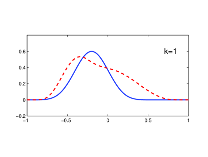
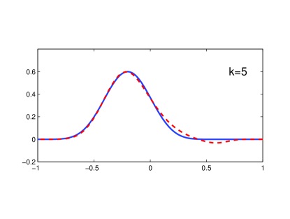
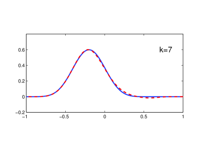
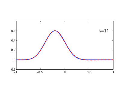
Figure 2: The reconstructed curve (dashed line) at $k=1,5,7,11,$ respectively, from $3\%$ noisy data with one incident direction $d=(\sin(\pi/3),-\cos(\pi/3))$, where the real curve is denoted by the solid line.

Example 2. In this example, we consider the case when the local perturbation of the infinite plane is under the $x_{1}$-axis with

$$h_{\Gamma}(x_{1})=-0.8\phi(({x_{1}-0.3})/{0.2}),$$

where $\phi$ is also given in Remark 5.1. In the inverse problem, the number of the spline basis functions is chosen to be $M=10$ and the total number of frequencies is chosen to be $N=9$. Figure 3 presents the reconstructed curves at $k=1,5,11,17,$ respectively, from $3\%$ noisy data with one incident direction $d=(\sin(\pi/3),-\cos(\pi/3))$.

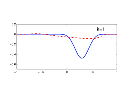
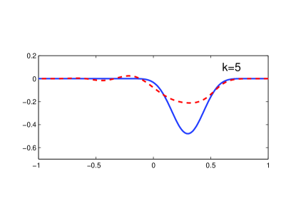
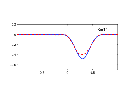
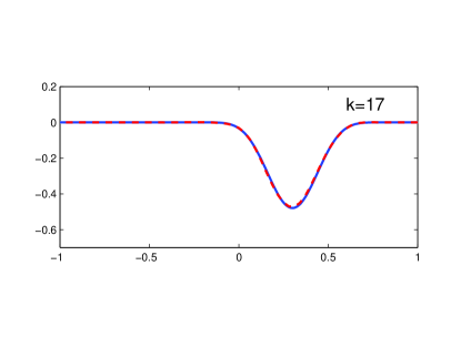
Figure 3: The reconstructed curve (dashed line) at $k=1,5,11,17,$ respectively, from $3\%$ noisy data with one incident direction $d=(\sin(\pi/3),-\cos(\pi/3))$, where the real curve is denoted by the solid line.

Example 3. The reconstruction considered in this example is a more challenging one with

$$h_{\Gamma}(x_{1})=\left\{\begin{array}[]{ll}\displaystyle\exp\left[16/(25x_{1}^{2}-16)\right]\sin(4\pi x_{1}),&|x_{1}|<4/5\\ \displaystyle 0,&|x_{1}|\geq 0\end{array}\right.$$

Here, we consider $10\%$ noisy data. In order to get a good reconstruction, the number of the spline basis functions is taken to be $M=20$ and the total number of frequencies is taken to be $N=15$. Figure 4 gives the reconstruction at $k=1,9,19,29$, respectively, with one incident direction $d=(0,-1)$ (normal incidence from the top).

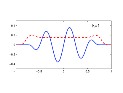
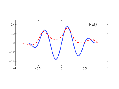
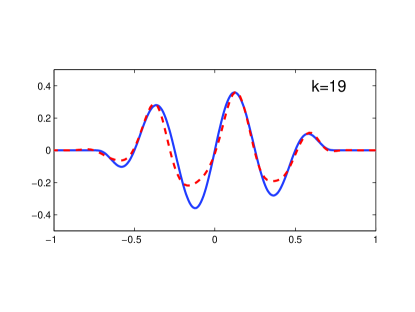
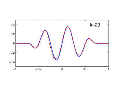
Figure 4: The reconstructed curve (dashed line) at $k=1,9,19,29$, respectively, from $10\%$ noisy data with normal incidence from the top, where the real curve is denoted by the solid line.

Example 4 (multi-scale profile). We now consider the multi-scale case with

$$h_{\Gamma}(x_{1})=\left\{\begin{array}[]{ll}\displaystyle\exp\left[16/(25x_{1}^{2}-16)\right]\left[0.5+0.1\sin(16\pi x_{1})\right],&|x_{1}|<4/5\\ \displaystyle 0,&|x_{1}|\geq 0.\end{array}\right.$$

This function has two scales: the macro-scale is represented by the function $0.5\exp[16/(25x_{1}^{2}-16)]$, and the micro-scale is represented by the function $0.1\exp[16/(25x_{1}^{2}-16)]\sin(16\pi x_{1})$. To capture the two-scale features of the profile, the number of spline basis functions is chosen to be $M=40$, and the total number of frequencies used is $N=30$. The reconstruction is obtained with $10\%$ noisy data using one incident plane wave with normal incidence from the top. Figure 5 presents the reconstructed profiles at $k=9,33,45,59$. From Figure 5 it is observed that the macro-scale features are captured when $k=9$ (Figure 5, top left), while the micro-scale features are captured at $k=59$ (Figure 5, bottom right). It is interesting to note that the resolution of the reconstruction does not improve much for $k\in[9,33]$ and then improves from a larger $k$ (e.g., $k=45$) until a sufficiently large $k$ (e.g., $k=59$) for which the whole local rough surface is accurately recovered even with $10\%$ noisy data. This indicates that our Newton algorithm with multiple frequency far-field data can give a stable and accurate reconstruction of multi-scale profiles with noise data as long as sufficiently high frequency data are used. This is similar to the reconstruction algorithm with multi-frequency near-field data developed in [4].

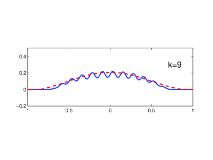
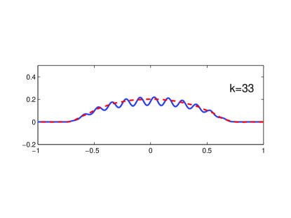
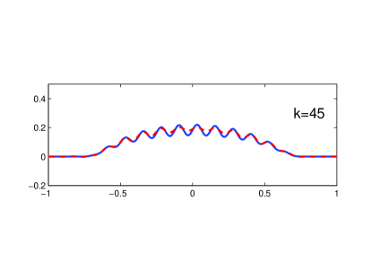
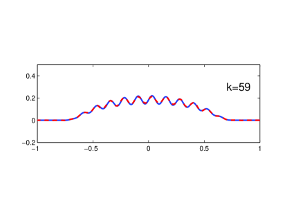
Figure 5: The reconstructed curve (dashed line) at $k=9,33,45,59$, respectively, from $10\%$ noisy data with normal incidence from the top, where the real curve is denoted by the solid line.

The above numerical results illustrate that the Newton iteration algorithm with multiple frequency data gives a stable and accurate reconstruction of the local perturbation of the infinite plane even in the presence of $10\%$ noise in measurements. From Figures 2-5 it is seen that the upper part of the locally rough surface can be recovered easily at lower frequencies; however, much higher frequencies are needed in order to recover the deep, lower part of the locally rough surface as well as the fine details of the micro-scale features of multi-scale profiles.

We are currently trying to extend the technique to the TM polarization case. Furthermore, it is anticipated that the reconstruction method can be generalized to the three-dimensional case.

References

- [1] H. Ammari, G. Bao and A. Wood, An integral equation method for the electromagnetic scattering from cavities, Math. Methods Appl. Sci. 23 (2000), 1057-1072.
- [2] G. Bao, J. Gao and P. Li, Analysis of direct and inverse cavity scattering problems, Numer. Math. Theor. Meth. Appl. 4 (2011), 419-442.
- [3] G. Bao and J. Lin, Near-field imaging of the surface displacement on an infinite ground plane, to appear in Inverse Problems Imaging.
- [4] G. Bao and J. Lin, Imaging of local surface displacement on an infinite ground plane: the multiple frequency case, SIAM J. Appl. Math. 71 (2011), 1733-1752.
- [5] G. Bao and J. Lin, Imaging of reflective surfaces by near-field optics, Optics Letters 37 (2012), 5027-5029.
- [6] G. Bao and W. Sun, A fast algorithm for the electromagnetic scattering from a large cavity, SIAM J. Sci. Comput. 27 (2005), 553-574.
- [7] C. Burkard and R. Potthast, A multi-section approach for rough surface reconstruction via the Kirsch–Kress scheme, Inverse Problems 26 (2010) 045007 (23pp).
- [8] S.N. Chandler-Widle and B. Zhang, A uniqueness result for scattering by infinite rough surfaces, SIAM J. Appl. Math. 58 (1998), 1774-1790.
- [9] S.N. Chandler-Wilde, C.R. Ross and B. Zhang, Scattering by infinite one-dimensional rough surfaces, Proc. R. Soc. London A 455 (1999), 3767-3787.
- [10] S.N. Chandler-Wilde and P. Monk, Existence, uniqueness and variational methods for scattering by unbounded rough surfaces, SIAM J. Math. Anal. 37 (2005), 598-618.
- [11] S.N. Chandler-Wilde, E. Heinemeyer and R. Potthast, A well-posed integral equation formulation for three-dimensional rough surface scattering, Proc. R. Soc. London A 462 (2006), 3683-3705.
- [12] S.N. Chandler-Wilde, E. Heinemeyer and R. Potthast, Acoustic scattering by mildly rough unbounded surfaces in three dimensions, SIAM J. Appl. Math. 66 (2006), 1002-1026.
- [13] S.N. Chandler-Wilde and J. Elschner, Variational approach in weighted Sobolev spaces to scattering by unbounded rough surfaces, SIAM J. Math. Anal. 42 (2010), 2554-2580.
- [14] S.N. Chandler-Wilde and C. Lines, A time domain point source method for inverse scattering by rough surfaces, Computing 75 (2005), 157-180.
- [15] R. Coifman, M. Goldberg, T. Hrycak, M. Israeli and V. Rokhlin, An improved operator expansion algorithm for direct and inverse scattering computations, Waves Random Media 9 (1999), 441-457.
- [16] D. Colton and R. Kress, Integral Equation Methods in Scattering Theory, John Wiley, New York, 1983.
- [17] D. Colton and R. Kress, Inverse Acoustic and Electromagnetic Scattering Theory (2nd edn), Springer, Berlin, 1998.
- [18] C. de Boor, A Practical Guide to Splines, Springer, New York, 2001.
- [19] J.A. DeSanto and R.J. Wombell, Reconstruction of rough surface profiles with the Kirchhoff approximation, J. Opt. Soc. Amer. A 8 (1991), 1892-1897.
- [20] J.A. DeSanto and R.J. Wombell, The reconstruction of shallow rough-surface profiles from scattered field data, Inverse Problems 7 (1991), L7-L12.
- [21] L. Feng and F. Ma, Uniqueness and local stability for the inverse scattering problem of determining the cavity, Science China A Math. 48 (2005), 1113-1123.
- [22] P. Henrici, Applied and Computational Complex Analysis Vol. 3, John Wiley, New York, 1986.
- [23] T. Hohage, Iterative Methods in Inverse Obstacle Scattering: Regularization Theory of Linear and Nonlinear Exponentially Ill-Posed Problems, PhD thesis, University of Linz, 1999.
- [24] R. Kress, A Nyström method for boundary integral equations in domain with corners, Numer. Math. 58 (1990), 145-161.
- [25] R. Kress, On the numerical solution of a hypersingular integral equation in scattering theory, J. Comp. Appl. Math. 61 (1995), 345-360.
- [26] R. Kress, Linear Integral Equations (2nd edn), Springer, New York, 1999.
- [27] R. Kress and T. Tran, Inverse scattering for a locally perturbed half-plane, Inverse Problems 16 (2000), 1541-1559.
- [28] P. Li, An inverse cavity problem for Maxwell’s equations, J. Differential Equations 252 (2012), 3209-3225.
- [29] C. Ruland, Ein Verfahren zur Lösung von Aussengebieten mit Ecken, Applic. Anal. 7 (1978), 69-79.
- [30] A. Willers, The Helmholtz equation in disturbed half-spaces, Math. Methods Appl. Sci. 9 (1987), 312-323.
- [31] B. Zhang and S.N. Chandler-Wilde, Integral equation methods for scattering by infinite rough surfaces, Math. Methods Appl. Sci. 26 (2003), 463-488.