Spin Liquid States at the Vicinity of Metal-Insulator Transition

Abstract

We study in this paper quantum spin liquid states (QSLs) at the vicinity of metal-insulator transition. Assuming that the low energy excitations in the QSLs are labeled by “spinon” occupation numbers with the same Fermi surface structure as in the corresponding metal (Fermi-liquid) side, we propose a phenomenological Landau-like low energy theory for the QSLs and show that the usual $U(1)$ QSLs is a representative member of this class of spin liquids. Based on our effective low energy theory, an alternative picture to the Brinkman-Rice picture of Mott metal-insulator transition is proposed. The charge, spin and thermal responses of QSLs are discussed under such a phenomenology.

I Introduction

Quantum spin liquid states (QSLs) in dimensions $d>1$ has been a long sought dream in condensed matter physics which has not been confirmed in realistic materials until rather recently.Lee08 These states are electronic Mott insulators that are not magnetically ordered down to the lowest temperature due to strong quantum mechanical fluctuations of spins and/or frustrated interaction. Various exotic properties have been proposed to exist in QSLs. For instance, charge neutral and spin-$\frac{1}{2}$ mobile objects, spinons, were proposed to emerge in such electronic states at low temperature accompanied by different kinds of (emerging) gauge fields. The spinons may be gapped or gapless and may obey either boson or fermion statistics. These new particles and gauge fields which characterize low energy behaviors of the system do not appear in the parent Hamiltonian and “emerge” as a result of strong correlation.

In the past few years, several experimental candidates for QSLs have been discovered that support the existence of gapless fermionic spinon excitations. The best studied example is a family of organic compounds $\kappa-$(ET)₂Cu₂(CN)₃ (ET)Kanoda03 and Pd(dmit)₂(EtMe₃Sb) (dmit salts)Itou08 . Both materials are Mott insulators in proximity to the metal-insulator transition because they become superconductor (ET) or metal (dmit) under modest pressure. Despite the large magnetic exchange $J\approx 250$ K observed in these systems, there is no experimental indication of long range magnetic ordering down to temperature $\sim 30~{}mK$. Linear temperature dependence of the specific heat and Pauli-like spin susceptibility were found in both materials at low temperature suggesting that the low energy excitations are spin-1/2 fermions with a Fermi surface.SYamashita ; Matsuda12 This Fermi liquid-like behavior is further supported by their Wilson ratios which are close to one. The thermal conductivity experiments on the ET salts found a large contribution to $\kappa$ beside phonons with $\kappa/T$ much reduced below 0.3 K,MYamashita09 while $\kappa/T$ approaches to a constant down to the lowest temperature in dmit salts.MYamashita10 All these experimental observations point to the scenario that the low lying excitations in these Mott insulators are mobile fermionic particles (spinons) that form a Fermi surface like their parent electrons ($U(1)$ spin liquid state). Besides ET and dmit-salts, the Kagome compound ZnCu₃(OH)₆Cl₂, the three dimensional hyper-Kagome material Na₄Ir₃O₈ and the newly discovered triangular compound Ba₃CuSb₂O₉ are also considered to be candidates for QSLs with gapless excitations.Kagome07 ; Takagi07 ; HDZhou2011

Several experiments were proposed to probe mobile spinons in the $U(1)$ spin liquid state. For example, giant magnetoresistance like experiment was designed to measure mobile spinons through oscillatory coupling between two ferromagnets via a quantum spin liquid spacer.Norman2009 The thermal Hall effect in insulating quantum magnets was proposed as an example of thermal transport of spinons, where different responses were used to distinguish between magnon- and spinon- transports.KNL2010 The spinon life time and mass as well as gauge fluctuations can be measured through sound attenuation experiment.YZhou2011 Despite all these proposals, a generic method to compare theoretical prediction of QSLs to experimental data is still missing at the phenomenological level.

The purpose of this paper is to build a generic phenomenological theory for spin liquids with (large) Fermi surfaces. Starting from the fact that these QSLs are electrical insulators but good thermal conductors, we propose a unified Fermi liquid type effective theory that describes both Fermi liquids and QSLs with large Fermi surfaces. The theoretical framework allows us to compute thermodynamics, transport and electromagnetic response of QSLs coherently and compare the results with experiments.

The paper is organized as follows. In Section II, we discuss our formulation of Landau’s Fermi liquid type effective theory for both Fermi liquid and spin liquid states. In Section III, we discuss electromagnetic response where we calculate both AC conductivity and dielectric function for the QSLs. In Section IV, the renormalization of thermodynamics quantities are discussed. In Section V, we discuss the transport equation for quasiparticles where the scattering amplitude and thermal conductivity are computed base on the transport equation. In Section VI, we point out the connection between our theory and $U(1)$ gauge theory and propose an alternative picture from Brinkman-Rice’s for the Mott metal-insulator transition. The important implication of the Pomeranchuk instability is pointed out. Section VII is devoted to the summary.

II Phenomenological theory: Landau’s Fermi liquid type effective theory

In a Fermi liquid, when electron-electron interactions are adiabatically turned on, the low energy excited states of interacting N-electron systems evolve in a continuous way, and therefore remain in one-to-one correspondence with the states of noninteracting N-electron systems. The same labeling scheme through fermion occupation number is assumed in the theories of $U(1)$ spin liquid state. we shall make the same assumption here when we consider general fermionic QSLs with finite spinon Fermi surfaces, although the one-to-one correspondence with the states of noninteracting electron systems is not protected by adiabaticity and should be viewed as an ansatz.

With this assumption the low energy excitations in the QSLs with finite spinon Fermi surfaces are labeled by the same occupation numbers as free fermions. The difference between Fermi liquids and QSLs is that the excitations in Fermi liquid are quasi-particles that carry both charges and spins, whereas the excitations in QSLs are expected to carry only spins. In particular, DC charge transport exists in Fermi liquid states, but vanishes in QSLs (insulators). Meanwhile, there exist large electronic contribution to thermal conductivity at low temperature in these insulating states because of mobile spin excitations. These two phenomena provide additional criteria to specifying the Fermi liquid type effective theory for QSLs.

The assumption that the low energy excitations in these QSLs are labeled by the same occupation numbers as free fermions suggests that the excitation energy $\Delta E=E-E_{G}$ for these states are also given by a Landau-type expressionPines ; Baym

$$\Delta E=\sum_{\mathrm{p\sigma}}\xi_{\mathrm{p}}\delta n_{\mathrm{p\sigma}}+\frac{1}{2}\sum_{\mathrm{pp}^{\prime}\sigma\sigma^{\prime}}f_{\mathrm{pp}^{\prime}}^{\sigma\sigma^{\prime}}\delta n_{\mathrm{p}\sigma}\delta n_{\mathrm{p}^{\prime}\sigma^{\prime}}+O(\delta n^{3}),$$ (1)

where $\xi_{\mathrm{p}}=\frac{\mathrm{p}^{2}}{2m^{\ast}}-\mu$ is the (single) spinon energy measured from the chemical potential $\mu$, $m^{\ast}$ is the spinon effective mass and $\sigma$ and $\sigma^{\prime}$ are spin indices. $\delta n_{\mathrm{\ p\sigma}}=n_{\mathrm{p\sigma}}-n_{\mathrm{p\sigma}}^{0}$ measures the departure of the spinon distribution function from the ground state distribution $n_{\mathrm{p}}^{0}=\theta(-\xi_{\mathrm{p}})$. $f_{\mathrm{pp}^{\prime}}^{\sigma\sigma^{\prime}}$ is the interaction energy between excited spinons. A spherical, rotational invariant Fermi surface is assumed here for simplicity. In this case we may write $f_{\mathrm{pp}^{\prime}}^{\sigma\sigma^{\prime}}$ in terms of spin symmetric and spin antisymmetric components $f_{\mathrm{pp}^{\prime}}^{\sigma\sigma^{\prime}}=f_{\mathrm{pp}^{\prime}}^{s}\delta_{\sigma\sigma^{\prime}}+f_{\mathrm{pp}^{\prime}}^{a}\sigma\sigma^{\prime}$. For isotropic systems, $f_{\mathrm{pp}^{\prime}}^{s(a)}$ depends only on the angle $\theta$ between $\mathrm{p}$ and $\mathrm{p}^{\prime}$ and we can expand $f_{\mathrm{pp}^{\prime}}^{s(a)}=\sum_{l=0}^{\infty}f_{l}^{s(a)}P_{l}(\cos\theta)$ at 3D and $f_{\mathrm{pp}^{\prime}}^{s(a)}=\sum_{l=0}^{\infty}f_{l}^{s(a)}\cos(l\theta)$ at 2D, where $P_{l}$’s are Legendre polynomials. The Landau parameters, defined by

$$F_{l}^{s(a)}=N(0)f_{l}^{s(a)},$$

provide a dimensionless measures of the strengths of the interactions between spinons on the Fermi surface, where $N(0)$ is the Fermi surface density of states. The low temperature properties of the QSLs are completely determined by the spinon mass $m^{\ast}$ and the interaction $f_{\mathrm{pp}^{\prime}}^{\sigma\sigma^{\prime}}$ (or $F_{l}^{s(a)}$) as in Fermi liquid theory.

Notice that the energy functional $\Delta E$ for our QSLs is so far identical to that for Fermi liquids. To describe QSLs, additional conditions have to be imposed to ensure that the excitations in the effective low energy theory carry zero charge. We propose and shall demonstrate in the following that the QSLs distinguish themselves from Fermi liquids by having a strong constraint on the Landau parameters $F_{1}^{s}$.

We start with the observation that the charge current $\mathbf{J}$ carried by quasi-particles in Fermi liquid theory (and in QSLs) is given by

$$\mathbf{J}=\frac{m}{m^{\ast}}(1+\frac{F_{1}^{s}}{d})\mathbf{J}^{(0)},$$ (2a)

where $$\mathbf{J}^{(0)} d \frac{m^{\ast}}{m}=1+\frac{F_{1}^{s}}{d} \frac{m^{\ast}}{m}\neq 1+\frac{F_{1}^{s}}{d} \mathbf{J}_{Q}$$ is the charge current carried by the corresponding non-interacting fermions and is the dimension. (See Appendix for the derivation of Eq.(2a).) For translational invariant systems, the charge current carried by quasi-particles is not renormalized and Baym . However, this is in general not valid for electrons in crystals where Galilean invariance is lost. In this case and the charge current carries by quasi-particles is renormalized by quasi-particle interaction. On the other hand, the thermal current is only renormalized by the effective mass in Fermi liquid theory,

$$\mathbf{J}_{Q}=\frac{m}{m^{\ast}}\mathbf{J}_{Q}^{(0)},$$ (2b)

where $$\mathbf{J}_{Q}^{(0)} 1+F_{1}^{s}/d\rightarrow 0 \frac{m^{\ast}}{m} \mathbf{J}\rightarrow 0 \mathbf{J}_{Q}\neq 0 F_{1}^{s} \frac{m^{\ast}}{m}$$ is the corresponding thermal current carried by non-interacting electrons. (See Appendix for details.) Thus, in the special case while remaining finite, and suggesting that the electronic system is in a special state where spin-1/2 quasi-particles do not carry charge due to interaction but they still carry entropy (i.e. electric insulating but thermal conducting). This is exactly what we expect for spinons in QSLs. We note that it is crucial that is independent of for this mechanism to work.

The charge carried by the quasiparticles (building blocks of our effective theory) and elementary excitations should be distinguished carefully in our theory. The building blocks (described by $\delta n_{p\sigma}$’s) are chargeful quasiparticles, whereas elementary excitations are eigenstates of Landau’s transport equation with charge renormalized by $1+F_{1}^{s}/d$ and becomes zero in the limit $\mathrm{q}=0$ and $\omega=0$. In general, charge degrees of freedom are recovered at finite q and $\omega$ as we shall see when we study electromagnetic responses of QSLs in next section.

III Electromagnetic responses

To put our argument in a more quantitative framework we study the electromagnetic responses of a Fermi liquid system with $1+F_{1}^{s}/d\rightarrow 0$. The charge and (transverse) current response functions are given by the standard Fermi liquid formsNg1 ; Pines ; Leggett

$$\chi_{d}(\mathrm{q},\omega)=\frac{\chi_{0d}(\mathrm{q},\omega)}{1-\left(F_{0}^{s}+\frac{F_{1}^{s}(\mathrm{q},\omega)}{d+F_{1}^{s}(\mathrm{q},\omega)}\frac{\omega^{2}}{q^{2}}\right)\frac{\chi_{0d}(\mathrm{q},\omega)}{N(0)}},$$ (3)

and

$$\chi_{t}(\mathrm{q},\omega)=\frac{\chi_{0t}(\mathrm{q},\omega)}{1-\frac{F_{1}^{s}(\mathrm{q},\omega)}{d+F_{1}^{s}(\mathrm{q},\omega)}\frac{\chi_{0t}(\mathrm{q},\omega)}{N(0)}},$$ (4)

where $\chi_{0d}(\mathrm{q},\omega)$ and $\chi_{0t}(\mathrm{q},\omega)$ are the density-density and (transverse) current-current response functions for a Fermi gas with effective mass $m^{\ast}$ but without Landau interactions, respectively. The longitudinal current-current response function $\chi_{l}$ is related to $\chi_{d}$ through

$$\chi_{d}(\mathrm{q},\omega)=(q^{2}/\omega^{2})\chi_{l}(\mathrm{q},\omega)$$

and the ac conductivity $\sigma_{l(t)}$ is related to $\chi_{l(t)}$ by

$$\sigma_{l(t)}(\mathrm{q},\omega)=e^{2}\chi_{l(t)}(\mathrm{q},\omega)/i\omega,$$

where $\mathrm{q}=|\vec{q}|$. In the singular limit $1+F_{1}^{s}/d\rightarrow 0$, it is clear that higher order $\mathrm{q},\omega$-dependent terms should be included in the Landau interaction to obtain finite results. Expanding at small $\mathrm{q}$ and $\omega$, we obtain

$$\frac{1+F_{1}^{s}(\mathrm{q},\omega)/d}{N(0)}\sim\alpha-\beta\omega^{2}+\gamma_{t}q_{t}^{2}+\gamma_{l}q_{l}^{2},$$ (5)

where $q_{t}\sim\nabla\times$ and $q_{l}\sim\nabla$ are associated the transverse (curl) and longitudinal (gradient) parts of the small $\vec{q}$ expansion. $\alpha=0$ in the QSLs. Putting this into the charge response function $\chi_{d}$, we find that to ensure that the system is in an incompressible (insulator) state, we must have $\gamma_{l}=0$. The other possibility $F_{0}^{s}\rightarrow\infty$ implies complete vanishing of charge responses in the insulating state.

With this parametrization we obtain for the ac conductivity at small $\omega$,

$$\sigma(\omega)=\frac{\omega\sigma_{0}\left(\omega\right)}{\omega-i\sigma_{0}\left(\omega\right)/\beta e^{2}},$$ (6)

where $\sigma_{0}(\omega)=e^{2}\chi_{0t}(0,\omega)/(i\omega)=e^{2}\chi_{0l}(0,\omega)/(i\omega)$. The last equality is valid as long as $F_{0}^{s}$ is finite. Eq. (6) was first obtained in the $U(1)$ gauge theory approach to spin liquid in a slightly different formnglee and predicts power law conductivity Re$[\sigma(\omega)]\sim\omega^{3.33}(\omega^{2})$ (at 2D) at frequency regime $\omega>(<)(1/\tau_{0},k_{B}T/\hbar)$, where $\tau_{0}$ is the elastic scattering timenglee . The dielectric function is given at small $\mathrm{q},\omega$ by

$$\varepsilon(\mathrm{q},\omega)=1-\frac{4\pi e^{2}}{q^{2}}\chi_{d}(\mathrm{q},\omega)\sim 1+4\pi\beta e^{2}+O(q^{2}),$$ (7)

also in agreement with the result obtained in $U(1)$ gauge theorynglee .

IV Thermodynamics

Our picture of QSLs has several immediate experimental consequences. We shall discuss theromadynamics of QSLs in this section and leave transport properties in next section.

One of important experimental evidences supporting the existence of gapless fermionic spinon exciations is linearly temperature dependent specific heat. The finite specific heat ratio indicates finite density of states at Fermi level. In Fermi liquid theory, the specific heat ratio $\gamma$ is renormalized by the effective mass $m^{\ast}$ through the density of statesPines , namely,

$$\gamma=\frac{C_{V}}{T}=\frac{m^{\ast}}{m}\frac{C_{V}^{(0)}}{T}=\frac{m^{\ast}}{m}\gamma^{(0)},$$

where $C_{V}^{(0)}$ and $\gamma^{(0)}$ are the specific heat and the specific heat ratio for the corresponding non-interacting electron gas respectively. Since $m^{\ast}/m$ remains finite in QSL phase, $\gamma$ is predicted to be finite at the QSLs.

The spin susceptibility $\chi_{P}$ will be renormalized by the spin antisymmetric Landau parameter $F_{0}^{a}$ as well as the effective mass $m^{\ast}$Pines . It gives rise to

$$\chi_{P}=\frac{m^{\ast}}{m}\frac{1}{1+F_{0}^{a}}\chi_{P}^{(0)},$$

where $\chi_{P}^{(0)}$ is the Pauli susceptibility for the corresponding non-interacting electron gas. It is clear that magnetic susceptibility $\chi_{P}$ is also non-singular in the QSLs.

Combining the specific heat ratio and spin susceptibility together, we find that the Wilson ratio

$$R=\frac{4\pi^{2}k_{B}^{2}\chi_{P}}{3(g\mu_{B})^{2}\gamma}\sim(1+F_{0}^{a})^{-1}$$

is generally of order $O(1)$, which is one of the experimental observations in QSLs.

The QSLs have zero compressibility as can be seen from the dielectric function (7).

V Transport properties

The transport properties in the QSLs can be computed using the Landau transport equation. We expect that the transport life-times will be dominated by scattering in the current-current channel which is the most singular scattering channel in the limit $1+\frac{F_{1}^{s}}{d}\rightarrow 0$. We shall show that the effect of scattering in this channel is equivalent to results obtained from $U(1)$ gauge theory.

In the Landau transport equation which is essentially a Boltzmann equation, the transition probability $W(1,2;3,4)$ for a two quasi-particles scattering process in an isotropic Fermi liquid, $1+2\rightarrow 3+4$ with $i\equiv(\mathrm{p}_{i},\sigma_{i})$, is given by $2\pi$ times the squared moduli of the quasi-particle scattering amplitude,

$$W(1,2;3,4)=2\pi|A(1,2;3,4)|^{2}.$$

We are interested in the situation that the momentum transfer $\mathrm{q}=\mathrm{p}_{1}-\mathrm{p}_{3}$ is small and $\mathrm{p}=\frac{1}{2}(\mathrm{p}_{1}+\mathrm{p}_{3})$ and $\mathrm{p}^{\prime}=\frac{1}{2}(\mathrm{p}_{2}+\mathrm{p}_{4})$ are close to the Fermi momentum $\mathrm{p}_{F}$ as shown in Fig. 1. In this case, the scattering amplitude depends mainly on the relative orientation of the vector $\mathrm{p}$, $\mathrm{p}^{\prime}$ and $\mathrm{q}$, and on the the energy transfer $\omega=\epsilon_{\mathrm{p+q/2}}-\epsilon_{\mathrm{p-q/2}}=\epsilon_{\mathrm{p}^{\prime}\mathrm{+q/2}}-\epsilon_{\mathrm{p}^{\prime}\mathrm{-q/2}}$. The transition probability can be written as

$$W(1,2;3,4)=2\pi|A_{\mathrm{pp}^{\prime}}(\mathrm{q},\omega=\epsilon_{\mathrm{p+q/2}}-\epsilon_{\mathrm{p-q/2}})|^{2}.$$

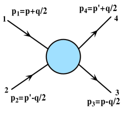
Figure 1: (Color Online) Two quasi-particle scattering in a Fermi liquid. Two in-going quasiparticles with momenta $\mathrm{p_{1}}$ and $\mathrm{p_{2}}$ interact with each other, resulting in two out-going quasiparticles with momenta $\mathrm{p_{3}}$ and $\mathrm{p_{4}}$. The momentum conservation requires that $\mathrm{p_{1}}+\mathrm{p_{2}}=\mathrm{p_{3}}+\mathrm{p_{4}}$. The momentum transfer is $\mathrm{q}=\mathrm{p}_{1}-\mathrm{p}_{3}=\mathrm{p}_{4}-\mathrm{p}_{2}$. By introducing $\mathrm{p}=\frac{1}{2}(\mathrm{p}_{1}+\mathrm{p}_{3})$ and $\mathrm{p}^{\prime}=\frac{1}{2}(\mathrm{p}_{2}+\mathrm{p}_{4})$, the four momenta $\mathrm{p_{1}}$, $\mathrm{p_{2}}$, $\mathrm{p_{3}}$ and $\mathrm{p_{4}}$ can be written in terms of $\mathrm{p}$, $\mathrm{p}^{\prime}$ and $\mathrm{q}$.

V.1 Quasi-particle scattering amplitude

We shall neglect the spin indices in the following for brevity. The spin-degeneracy factor 2 will be inserted when the need arises. The quasi-particle scattering amplitude $A_{\mathrm{pp}^{\prime}}\left(\mathrm{q},\omega\right)$ is then given by the following equation,

$$A_{\mathrm{pp}^{\prime}}\left(\mathrm{q},\omega\right)-\sum_{\mathrm{p}^{\prime\prime}}f_{\mathrm{pp}^{\prime\prime}}\chi_{0\mathrm{p}^{\prime\prime}}\left(\mathrm{q},\omega\right)A_{\mathrm{p}^{\prime\prime}\mathrm{p}^{\prime}}\left(\mathrm{q},\omega\right)=f_{\mathrm{pp}^{\prime}},$$

where $\chi_{0\mathrm{p}}\left(\mathrm{q},\omega\right)$ is the susceptibility

$$\chi_{0\mathrm{p}}\left(\mathrm{q},\omega\right)=\frac{n_{\mathrm{p}-\mathrm{q}/2}^{0}-n_{\mathrm{p}+\mathrm{q}/2}^{0}}{\omega+\xi_{\mathrm{p}-\mathrm{q}/2}-\xi_{\mathrm{p}+\mathrm{q}/2}}\simeq\frac{\mathbf{q}\cdot\mathbf{v}_{\mathrm{p}}}{\mathrm{q}\cdot\mathrm{v}_{\mathrm{p}}-\omega}\frac{\partial n_{\mathrm{p}}^{0}}{\partial\xi_{\mathrm{p}}},$$

with $n_{\mathrm{k}}^{0}=n_{F}(\xi_{\mathrm{k}})$. We shall assume that the scattering is dominating by the $l=1$ channel and approximate

$$f_{\mathrm{pp}^{\prime}}\sim\frac{\mathbf{p}\cdot\mathbf{p}^{\prime}}{p_{F}^{2}}f_{1}^{s}.$$

It is then easy to show that

$$A_{\mathrm{pp}^{\prime}}\left(\mathrm{q},\omega\right)=\frac{\mathbf{p}\cdot\mathbf{p}^{\prime}}{p_{F}^{2}}\frac{f_{1}^{s}}{1-\chi_{1}(\mathrm{q},\omega)f_{1}^{s}},$$ (8)

where

$$\chi_{1}(\mathrm{q},\omega)=\frac{1}{V}\sum_{\mathrm{p}}\frac{p^{2}}{p_{F}^{2}d}\left(\frac{n_{\mathrm{p}-\mathrm{q}/2}^{0}-n_{\mathrm{p}+\mathrm{q}/2}^{0}}{\omega+\xi_{\mathrm{p}-\mathrm{q}/2}-\xi_{\mathrm{p}+\mathrm{q}/2}+i\delta}\right).$$

For small $\left(\mathrm{q},\omega\right)$ we have

$$\chi_{1}(\mathrm{q},\omega)\sim-\frac{N(0)}{d}\left[1+ig(d)\frac{\omega}{v_{F}q}\right]$$

for $\omega\ll v_{F}q$, where $q=|\mathrm{q}|$, $g(2)=1$ and $g(3)=\frac{\pi}{2}$. In the limit $N(0)f_{1}^{s}/d=F_{1}^{s}/d\rightarrow-1$, using the expansion (see Eq.(5))

$$f_{1}^{s}=\frac{d}{N(0)}\left(-1-\beta\omega^{2}+\gamma_{t}q^{2}\right),$$

we obtain

$$A_{\mathrm{pp}^{\prime}}\left(\mathrm{q},\omega\right)\simeq\frac{d}{N(0)}\frac{\mathbf{p}\cdot\mathbf{p}^{\prime}}{p_{F}^{2}}\frac{1}{-ig\frac{\omega}{v_{F}q}+\gamma_{t}q^{2}},$$ (9)

where the last factor is exact the gauge field propagator in $U(1)$ gauge theory.

V.2 Thermal conductivity

Following PethickPethick , we use a variational approachZiman to derive the thermal conductivity $\kappa$ from the transport equation. The thermal resistivity for a Fermi liquid is given by

$$\frac{1}{\kappa} = \frac{1}{4}\sum_{1,2,3,4}W(1,2;3,4)n_{1}^{0}n_{2}^{0}(1-n_{3}^{0})(1-n_{4}^{0})$$ (10)

$$\times(\phi_{1}+\phi_{2}-\phi_{3}-\phi_{4})^{2}\left(\sum_{1}\phi_{1}\xi_{1}\mathbf{v}_{1}\cdot\mathbf{u}\frac{\partial n_{1}^{0}}{\partial\epsilon_{1}}\right)^{-2}$$

$$\times\delta(\epsilon_{1}+\epsilon_{2}-\epsilon_{3}-\epsilon_{4})\delta_{\sigma_{1}+\sigma_{2},\sigma_{3}+\sigma_{4}}\delta_{\mathrm{p}_{1}+\mathrm{p}_{2},\mathrm{p}_{3}+\mathrm{p}_{4}},$$

where $n_{i}^{0}=n_{F}(\xi_{i})$ is the Fermi distribution function with $i=1,2,3,4$, $\xi_{i}=\epsilon_{i}-\mu$, $\phi_{i}$ is defined by $n_{i}=n_{i}^{0}-\phi_{i}\frac{\partial n_{i}^{0}}{\partial\epsilon_{i}}$, $\mathrm{v}_{i}$ is the quasiparticle velocity, u is an arbitrary unit vector along which the temperature gradient $\nabla T$ is applied.

We shall make the usuall approximation $\phi_{i}=\xi_{i}\mathbf{v}_{i}\cdot\mathbf{u}$. To the order we are working with the approximation that the quasi-particle velocity may be replaced by $v_{F}$ and

$$\sum_{1}\phi_{1}\xi_{1}\mathbf{v}_{1}\cdot\mathbf{u}\frac{\partial n_{1}^{0}}{\partial\epsilon_{1}} = \sum_{1}\left(\xi_{1}\mathbf{v}_{1}\cdot\mathbf{u}\right)^{2}\frac{\partial n_{1}^{0}}{\partial\epsilon_{1}}$$

$$= \frac{4m^{\ast}N(0)}{d}\int d\xi(\xi+\mu)\xi^{2}\frac{\partial n^{0}(\xi)}{\partial\xi}$$

$$= -\frac{4m^{\ast}N(0)}{d}\frac{\pi}{3}\epsilon_{F}(k_{B}T)^{2}$$

$$= -\frac{2\pi}{3}\frac{n}{m^{\ast}}(k_{B}T)^{2},$$

where $n$ is the fermion density and the relation $d(n/m^{\ast})=N(0)v_{F}^{2}$ is used.

Introducing $\bar{\xi}_{\mathrm{p}}=\frac{1}{2}(\xi_{\mathrm{p+q/2}}+\xi_{\mathrm{p-q/2}})$ and using the conditions $\mathrm{q}=\mathrm{p}_{1}-\mathrm{p}_{3}=\mathrm{p}_{4}-\mathrm{p}_{2}$ and $\omega=\epsilon_{\mathrm{p+q/2}}-\epsilon_{\mathrm{p-q/2}}=\epsilon_{\mathrm{p}^{\prime}\mathrm{+q/2}}-\epsilon_{\mathrm{p}^{\prime}\mathrm{-q/2}}$, we have

$$m^{\ast}\left(\xi_{1}\mathbf{v}_{1}+\xi_{2}\mathbf{v}_{2}-\xi_{3}\mathbf{v}_{3}-\xi_{4}\mathbf{v}_{4}\right)$$

$$= \left(\bar{\xi}_{\mathrm{p}}+\omega/2\right)\left(\mathbf{p}+\mathbf{q}/2\right)+\left(\bar{\xi}_{\mathrm{p}^{\prime}}-\omega/2\right)\left(\mathbf{p}^{\prime}-\mathbf{q}/2\right)$$

$$-\left(\bar{\xi}_{\mathrm{p}}-\omega/2\right)\left(\mathbf{p}-\mathbf{q}/2\right)-\left(\bar{\xi}_{\mathrm{p}^{\prime}}+\omega/2\right)\left(\mathbf{p}^{\prime}+\mathbf{q}/2\right)$$

$$= \left(\bar{\xi}_{\mathrm{p}}-\bar{\xi}_{\mathrm{p}^{\prime}}\right)\mathbf{q+}\omega\left(\mathbf{p}-\mathbf{p}^{\prime}\right)$$

$$= \left(\xi_{\mathrm{p}}-\xi_{\mathrm{p}^{\prime}}\right)\mathbf{q+}\omega\left(\mathbf{p}-\mathbf{p}^{\prime}\right),$$

and

$$\langle\left(\phi_{1}+\phi_{2}-\phi_{3}-\phi_{4}\right)^{2}\rangle$$

$$= \langle\left[\left(\xi_{1}\mathbf{v}_{1}+\xi_{2}\mathbf{v}_{2}-\xi_{3}\mathbf{v}_{3}-\xi_{4}\mathbf{v}_{4}\right)\cdot\mathbf{u}\right]^{2}\rangle$$

$$= \frac{1}{d}\left(\xi_{1}\mathbf{v}_{1}+\xi_{2}\mathbf{v}_{2}-\xi_{3}\mathbf{v}_{3}-\xi_{4}\mathbf{v}_{4}\right)^{2}$$

$$= \frac{1}{m^{\ast 2}d}\left[(\xi_{\mathrm{p}}-\xi_{\mathrm{p}^{\prime}})\mathbf{q+}(\mathbf{p}-\mathbf{p}^{\prime})\omega\right]^{2},$$

where $\langle\cdots\rangle$ means averaging over different u.

Putting $A_{\mathrm{pp}^{\prime}}\left(\mathrm{q},\omega\right)$ into (10), and using the identity $n_{1}^{0}(1-n_{3}^{0})=(n_{1}^{0}-n_{3}^{0})/[1-e^{\beta(\epsilon_{1}-\epsilon_{3})}]$, we obtain

$$\frac{1}{\kappa} \propto \frac{1}{T^{4}}\sum_{\mathrm{q,p,p}^{\prime}}\int d\omega\frac{|A_{\mathrm{pp}^{\prime}}\left(\mathrm{q},\omega\right)|^{2}}{(e^{\beta\omega}-1)(1-e^{-\beta\omega})}$$

$$\times[n_{F}(\xi_{\mathrm{p-q/2}})-n_{F}(\xi_{\mathrm{p+q/2}})]\delta(\omega-\mathbf{p}\cdot\mathbf{q}/m^{\ast})$$

$$\times[n_{F}(\xi_{\mathrm{p}^{\prime}\mathrm{+q/2}})-n_{F}(\xi_{\mathrm{p}^{\prime}\mathrm{-q/2}})]\delta(\omega-\mathbf{p}^{\prime}\cdot\mathbf{q}/m^{\ast})$$

$$\times[(\xi_{\mathrm{p}}-\xi_{\mathrm{p}^{\prime}})^{2}q^{2}\mathbf{+(p}-\mathbf{p}^{\prime})^{2}\omega^{2}],$$

where we have used the $\delta$-functions to simplify the expression. Replacing $n_{F}(\xi_{\mathrm{p-q/2}})-n_{F}(\xi_{\mathrm{p+q/2}})$ and $n_{F}(\xi_{\mathrm{p}^{\prime}\mathrm{+q/2}})-n_{F}(\xi_{\mathrm{p}^{\prime}\mathrm{-q/2}})$ by $\omega\frac{\partial n_{F}}{\partial\xi_{\mathrm{p}}}$ and $\omega\frac{\partial n_{F}}{\partial\xi_{\mathrm{p}^{\prime}}}$ respectively which is valid at small $\mathrm{q}$ and $\omega$, we obtain

$$\frac{1}{\kappa} \propto \frac{1}{T^{4}}\sum_{\mathrm{q,p,p}^{\prime}}\int d\omega\frac{\omega^{2}|A_{\mathrm{pp}^{\prime}}\left(\mathrm{q},\omega\right)|^{2}}{(e^{\beta\omega}-1)(1-e^{-\beta\omega})}$$

$$\times\frac{\partial n_{F}}{\partial\xi_{\mathrm{p}}}\frac{\partial n_{F}}{\partial\xi_{\mathrm{p}^{\prime}}}\delta(\omega-\mathbf{p}\cdot\mathbf{q}/m^{\ast})\delta(\omega-\mathbf{p}^{\prime}\cdot\mathbf{q}/m^{\ast})$$

$$\times[(\xi_{\mathrm{p}}-\xi_{\mathrm{p}^{\prime}})^{2}q^{2}\mathbf{+(p}-\mathbf{p}^{\prime})^{2}\omega^{2}].$$

Let $\theta(\theta^{\prime})$ be the angle between $\mathbf{p}(\mathbf{p}^{\prime})$ and $\mathbf{q}$, and integrating over $\xi_{\mathrm{p}}$ and $\xi_{\mathrm{p}^{\prime}}$, we obtain

$$\frac{1}{\kappa} \propto \frac{1}{T^{4}}\sum_{\mathrm{q,\hat{p},\hat{p}}^{\prime}}\int d\omega\frac{\omega^{4}|A_{\mathrm{pp}^{\prime}}\left(\mathrm{q},\omega\right)|^{2}}{(e^{\beta\omega}-1)(1-e^{-\beta\omega})}\mathbf{(\hat{p}}-\mathbf{\hat{p}}^{\prime})^{2}$$

$$\times\delta(\omega-qv_{F}\cos\theta)\delta(\omega-qv_{F}\cos\theta^{\prime}).$$

Assuming that the scattering is dominated by $F_{1}^{s}$ channel and using Eq.(9), we obtain

$$\frac{1}{\kappa} \propto \frac{1}{T^{4}}\sum_{\mathrm{q}}\int d\omega\frac{\omega^{4}}{(e^{\beta\omega}-1)(1-e^{-\beta\omega})}\frac{1}{g^{2}\frac{\omega^{2}}{v_{F}^{2}q^{2}}+\gamma_{t}^{2}q^{4}}$$

$$\propto \frac{1}{T^{4}}\int d\omega\frac{\omega^{4}}{(e^{\beta\omega}-1)(1-e^{-\beta\omega})}\omega^{-(4-d)/3}$$

$$\propto \left(\frac{k_{B}T}{\epsilon_{F}}\right)^{(d-1)/3},$$

$\epsilon_{F}=p_{F}^{2}/2m^{\ast}$ is the spinon Fermi energy. The expression represents the thermal resistivity coming from inelastic scattering between fermions. At low temperature the inelastic scattering is cut off by elastic impurity scattering rate $1/\tau_{0}$, which gives rise to

$$\frac{\kappa_{\text{el}}}{T}=\frac{1}{d}\gamma^{\ast}v_{F}^{2}\tau_{0},$$

where $\gamma^{\ast}=C_{V}/T$ is the specific heat ratio, and $v_{F}$ is the spinon Fermi velocity. The total thermal conductivity is therefore given by

$$\frac{\kappa}{T}\propto\max\left[\frac{\hbar}{k_{B}^{2}}\left(\frac{k_{B}T}{\epsilon_{F}}\right)^{(4-d)/3},\frac{d}{\gamma^{\ast}v_{F}^{2}}\frac{1}{\tau_{0}}\right]^{-1}.$$

The same result is obtained in U(1) gauge theory at 2D.Nave07

VI Discussions

VI.1 Relation to the $U(1)$ gauge theory

The U(1) spin liquid is actually a member of the QSLs described by our phenomenology keeping scattering in the $l=0,1$ channels only. To show this we start with a Landau Fermi liquid with interaction parameters $F_{0}^{s}$ and $F_{1}^{s}(q,\omega)$ only. The long-wavelength and low dynamics of the Fermi liquid is described by an effective Lagrangian

$$L_{\text{eff}}=\sum_{\mathrm{k},\sigma}\left[c_{\mathrm{k}\sigma}^{\dagger}(i\frac{\partial}{\partial t}-\xi_{\mathrm{k}})c_{\mathrm{k}\sigma}-H^{\prime}(c^{{\dagger}},c)\right],$$ (11)

where $c_{\mathrm{k}\sigma}^{\dagger}(c_{\mathrm{k}\sigma})$ are spin-$\sigma$ fermion creation (annihilation) operators with momentum $\mathrm{k}$, and

$$H^{\prime}(c^{{\dagger}},c)=\frac{1}{2N(0)}\sum_{q}\left[\frac{F_{1}^{s}}{v_{F}^{2}}\mathbf{j}(q)\cdot\mathbf{j}(-q)+F_{0}^{s}n(q)n(-q)\right]$$ (12)

describes the current-current and density-density interactions between quasi-particlesLeggett , where $q=(\mathrm{q},\omega)$ and $v_{F}=\hbar k_{F}/m^{\ast}$ is the Fermi velocity.

The current- and density- interactions can be decoupled by introducing fictitious gauge potentials $\mathbf{a}$ and $\varphi$ (Hubbard-Stratonovich transformation) with

$$H^{\prime}(c^{{\dagger}},c)\rightarrow\sum_{q}\left[\mathbf{j}\cdot\mathbf{a}+n\varphi-{\frac{1}{2}}\left(\frac{n}{m^{\ast}}\frac{d}{F_{1}^{s}}\mathbf{a}^{2}+\frac{N(0)}{F_{0}^{s}}\varphi^{2}\right)\right],$$ (13)

where $n$ is fermion density. We have used the equality $d(n/m^{\ast})=N(0)v_{F}^{2}$ in writing down Eq. (13).

The Lagrangian (11) and (13) can be rewritten in the standard form of $U(1)$ gauge theory by noting that the fermion current is given in this representation by

$$\mathbf{j}=\frac{-i}{2m^{\ast}}\sum_{\sigma}\left[\psi_{\sigma}^{{\dagger}}\nabla\psi_{\sigma}-(\nabla\psi_{\sigma}^{\dagger})\psi_{\sigma}\right]-\frac{n}{m^{\ast}}\mathbf{a},$$

where $\psi_{\sigma}(\mathrm{r})=\int e^{-i\mathrm{k\cdot r}}c_{\mathrm{k}\sigma}$ in the Fourier transform of $c_{\mathrm{k}\sigma}$. The Lagrangian can be written as

$$L=\sum_{\sigma}\int d^{d}\mathrm{r}\left[\psi_{\sigma}^{\dagger}(i\frac{\partial}{\partial t}-\varphi)\psi_{\sigma}-H(\psi_{\sigma}^{\dagger},\psi_{\sigma})\right]+L(\varphi,\mathbf{a}),$$ (14a)

where

$$H(\psi_{\sigma}^{\dagger},\psi_{\sigma})=\frac{1}{2m^{\ast}}|(\nabla-i\mathbf{a})\psi_{\sigma}|^{2}$$ (14b)

and

$$L(\varphi,\mathbf{a})={\frac{1}{2}}\int d^{d}\mathrm{r}\left[\frac{n}{m^{\ast}}(1+\frac{d}{F_{1}^{s}})\mathbf{a}^{2}+\frac{N(0)}{F_{0}^{s}}\varphi^{2}\right].$$ (14c)

Notice how the $${\frac{n}{2m^{\ast}}}\mathbf{a}^{2} L(\varphi,\mathbf{a}) H(\psi_{\sigma}^{{\dagger}},\psi_{\sigma})$$ term in arises from the introduction of diamagnetic term in .

Using Eq. (5), we find that in the small $q$ limit, the transverse part of $L(\varphi,\mathbf{a})$ is given in the spin liquid state by

$$L_{t}(\varphi,\mathbf{a})=-\frac{n}{2m^{\ast}}\int d^{d}\mathrm{r}\left[\beta(\frac{\partial\mathbf{a}}{\partial t})^{2}-\gamma_{t}(\nabla\times\mathbf{a})^{2}\right].$$ (15)

The longitudinal part of the gauge potential $\varphi$ is screened as long as $F_{0}^{s}\neq 0$. Lagrangian (14) together with (15) is the standard Lagrangian used to describe $U(1)$ QSLs. It is interesting to note that a nonzero $1+\frac{F_{1}^{s}(0,0)}{d}$ leads to a mass term for the gauge field $\mathbf{a}$, in agreement with slave-boson/rotor approaches where a metallic state appears with condensation of bosons/rotorsLee05 ; Ng1 .

VI.2 Alternative picture of Mott transition

The close relation between Fermi liquid and spin-liquid states suggests that the (zero temperature) metal-insulator transition between the two states is characterized by the change of Landau parameter $1+F_{1}^{s}(0,0)/d\rightarrow 0^{+}$ across the transition. The nature of metal-insulator transition within the Fermi liquid framework was first addressed by Brinkman and RiceBrinkmanRice where they proposed that a metal-insulator (Mott) transition is indicated by diverging effective mass ${\frac{m^{\ast}}{m}}\rightarrow\infty$ and inverse compressibility $\kappa\rightarrow 0$ at the Mott transition point, with correspondingly a vanishing quasi-particle renormalization weight $Z\sim{\frac{m}{m^{\ast}}}\rightarrow 0$. The diverging effective mass and vanishing quasi-particle weight suggest that the Fermi liquid state is destroyed at the Mott transition, and the Mott insulator state is distinct from the Fermi liquid state at the metal side.

Here we propose an alternative picture where the Fermi surface is not destroyed but the quasiparticles are converted into spinons at the Mott transition. In particular, the effective mass $m^{\ast}/m$ may not diverge at the metal-insulator transition although $Z\rightarrow 0$ in this picture. A schematic phase diagram for the Mott (metal-QSLs) transition is presented in Fig. (2) where we imagine a Hubbard type Hamiltonian with hopping $t$ and on-site Coulomb repulsion $U$. The system is driven to a Mott insulator state at zero temperature at $U=U_{c}$, where $1+F_{1}^{s}(U>U_{c})/d=0$. Our picture is supported by the experimental fact that the potential candidates for the $U(1)$ QSLs with large Fermi surfaces (ET and dmit salts) are all closed to the metal-insulator transition. We caution that in general a finite ($T\neq 0$) region exists around the Mott transition point where the physics is dominated by critical fluctuations and our phenomenological theory is not applicable. We note that an alternative phenomenology for Mott transition from a semi-microscopic starting pointSenthil has qualitatively similar conclusion as our present work. The relation between the two works is not clear at present.

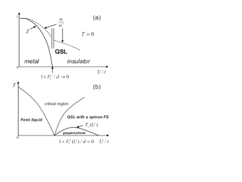
Figure 2: (a) Schematic zero temperature phase diagram for Mott transition. $U$ is the Hubbard interaction strength and $t$ is the hopping integral. The electron quasiparticle weight and quasi-particle charge current $\sim 1+F_{1}^{s}/d$ vanishes at the critical point while the effective mass remains finite. (b) Schematic phase diagram showing finite temperature crossovers and possible instability toward gapped phases at lower temperature. There exists a (finite temperature) critical region around $U_{c}$ where our phenomenological theory is not applicable.

VI.3 Pomeranchuk instability

Experienced researchers in Fermi liquid theory will recognize that the point $1+F_{1}^{s}/d=0$ is in fact a critical point in Fermi liquid theory. The Fermi surface is unstable with respect to deformation when $1+F_{1}^{s}/d<0$. The stability of the $1+F_{1}^{s}/d=0$ point is required in QSLs where quasi-particles (spinons) become chargeless. The resulting QSLs we obtain here are marginally stable because of large critical fluctuations. The large critical fluctuations give rise to singular corrections to thermodynamics quantities (specific heat for example) and transport coefficients (various scattering lifetimes) at two dimensions as first pointed out in $U(1)$ gauge theory. The Pomeranchuk criticality is an alternative way to express these results.

The presence of Pomeranchuk criticality suggests that QSLs with large Fermi surfaces are in general rather susceptible to formation of other more stable QSLs at lower temperature, like the $Z_{2}$ QSLs or valence bond solid (VBS) states that gap out part or the whole Fermi surface. The resulting phase diagram at the vicinity of Mott transition thus has the generic feature shown in Fig.(2b), where the system is driven into a gapped QSL at low temperature $T<T_{c}(U)$ at the insulating side. The nature of the low temperature QSLs depends on the microscopic details of the system and cannot be determined from our phenomenology. Our theory is applicable at $T>T_{c}(U)$, when the spin liquid is still in the large-Fermi surface phase.

VII Conclusion

In summary, we formulate a Fermi liquid type phenomenological theory for quantum spin liquid states in the vicinity of metal-insulator transition. The phenomenology takes into account the fact that DC electrical current and compressibility vanishes while thermal current keeps finite in QSLs. Physically, the phenomenology implies that the charge degrees of freedom of quasiparticles are frozen at $\mathrm{q}=0$ and $\omega=0$. Finite specific heat ratio, spin susceptibility and the fact Wilson ration is of order of unity indicate spin degrees of freedom are still active in this limit. The frozen charge degrees of freedom are recovered at finite q and $\omega$ as indicated by the power-law $\omega^{\eta}$-dependent AC conductivity. We also show that the $U(1)$ spin liquids is a member of the class of QSLs described by our phenomenology. We also propose an alternative picture of Mott transition and discuss the phase diagram.

TKN is supported by HKRGC through grant HKUST03/CRF09 and GRF 603410. YZ is supported by National Basic Research Program of China (973 Program, No.2011CBA00103/2014CB921201), NSFC (No.11074218/11374256) and the Fundamental Research Funds for the Central Universities in China. He also thanks the Institute for Advanced Studies, HKUST for its hospitality, where this work is completed.

Appendix A Renormalized currents

In this appendix we derive the renormalized currents in Fermi liquid theory ((Eq.(2a) and (2b)) in the main text). The local equilibrium quasi-particle occupation numbers and their fluctuations have to be considered carefully. The excitation energy of an additional quasiparticle with momentum $\mathrm{p}$ is given by

$$\tilde{\epsilon}_{\mathrm{p}}=\epsilon_{\mathrm{p}}+\sum_{\mathrm{p}^{\prime}}f_{\mathrm{pp}^{\prime}}^{s}\delta n_{\mathrm{p}^{\prime}},$$

where $\epsilon_{\mathrm{p}}=\frac{p^{2}}{2m^{\ast}}$. The corresponding local equilibrium occupation number is $\tilde{n}_{\mathrm{p}}^{0}\equiv n_{F}\left(\tilde{\epsilon}_{\mathrm{p}}-\mu\right)$, and the departure from local equilibrium reads

$$\delta\tilde{n}_{\mathrm{p}} = n_{\mathrm{p}}-\tilde{n}_{\mathrm{p}}^{0}$$

$$= \delta n_{\mathrm{p}}-\frac{\partial n^{0}}{\partial\epsilon_{\mathrm{p}}}\sum_{\mathrm{p}^{\prime}}f_{\mathrm{pp}^{\prime}}^{s}\delta n_{\mathrm{p}^{\prime}},$$

where $\delta n_{\mathrm{p}}=n_{\mathrm{p}}-n_{\mathrm{p}}^{0}$. The charge current $\mathrm{J}$ carried by quasiparticles is related to the particle density by the conservation law,

$$\frac{\partial\rho}{\partial t}+\nabla_{\mathrm{r}}\cdot\mathbf{J}=0.$$

The density fluctuation $\delta\rho\left(\mathrm{r},t\right)$ should be expressed in terms of the sum of $\delta\tilde{n}_{\mathrm{p}}\left(\mathrm{r},t\right)$ (i.e. fluctuation away from local equilibirum),

$$\delta\rho\left(\mathrm{r},t\right)=\sum_{\mathrm{p}}\delta\tilde{n}_{\mathrm{p}}\left(\mathrm{r},t\right)$$

and

$$\frac{\partial}{\partial t}\delta\rho+\nabla_{\mathrm{r}}\cdot\sum_{\mathrm{p}}\delta\tilde{n}_{\mathrm{p}}\mathbf{v}_{\mathrm{p}}=0.$$

Therefore,

$$\mathbf{J}=\sum_{\mathrm{p}}\delta\tilde{n}_{\mathrm{p}}\mathbf{v}_{\mathrm{p}}=\sum_{\mathrm{p}}\delta n_{\mathrm{p}}\mathbf{j}_{\mathrm{p}},$$

where

$$\mathbf{j}_{\mathrm{p}}=\mathbf{v}_{\mathrm{p}}-\sum_{\mathrm{p}^{\prime}}f_{\mathrm{pp}^{\prime}}^{s}\frac{\partial n^{0}}{\partial\epsilon_{\mathrm{p}^{\prime}}}\mathbf{v}_{\mathrm{p}^{\prime}}.$$

Using the relation

$$\sum_{\mathrm{p}^{\prime}}\frac{\partial n^{0}}{\partial\epsilon_{\mathrm{p}^{\prime}}}f_{\mathrm{pp}^{\prime}}\mathbf{v}_{\mathrm{p}^{\prime}} = \sum_{\mathrm{p}^{\prime}}\frac{\partial n^{0}}{\partial\epsilon_{\mathrm{p}^{\prime}}}N_{F}^{-1}\sum_{l}F_{l}^{s}P_{l}\left(\cos\theta\right)\mathbf{v}_{\mathrm{p}^{\prime}}$$

$$= \frac{1}{d}F_{1}^{s}\mathbf{v}_{\mathrm{p}}\int d\epsilon^{\prime}\frac{\partial n^{0}}{\partial\epsilon^{\prime}}=\frac{1}{d}F_{1}^{s}\mathbf{v}_{\mathrm{p}},$$

where $N_{F}=N\left(0\right)$, we find that the renormalized charge current is

$$\mathbf{J}=\frac{m}{m^{\ast}}(1+\frac{1}{d}F_{1}^{s})\mathbf{J}^{(0)},$$

when $\mathbf{J}^{0}$ is the electric current in the absence of interaction. Notice that $P_{l}\left(\cos\theta\right)$ is replaced by $\cos\left(l\theta\right)$ at 2D.

Similarly the thermal (energy) current $\mathbf{J}_{Q}$ is given by

$$\mathbf{J}_{Q} = \sum_{\mathrm{p}}\delta\tilde{n}_{\mathrm{p}}\left(\epsilon_{\mathrm{p}}-\mu\right)\mathbf{v}_{\mathrm{p}}$$

$$= \sum_{\mathrm{p}}\left(\epsilon_{\mathrm{p}}-\mu\right)\mathbf{v}_{\mathrm{p}}(\delta n_{\mathrm{p}}-\sum_{\mathrm{p}^{\prime}}\frac{\partial n^{0}}{\partial\epsilon_{\mathrm{p}}}f_{\mathrm{pp}^{\prime}}\delta n_{\mathrm{p}^{\prime}})$$

$$= \sum_{\mathrm{p}}\delta n_{\mathrm{p}}[\left(\epsilon_{\mathrm{p}}-\mu\right)\mathbf{v}_{\mathrm{p}}-\sum_{\mathrm{p}^{\prime}}\frac{\partial n^{0}}{\partial\epsilon_{\mathrm{p}^{\prime}}}f_{\mathrm{pp}^{\prime}}\left(\epsilon_{\mathrm{p}^{\prime}}-\mu\right)\mathbf{v}_{\mathrm{p}^{\prime}}].$$

Notice that

$$\sum_{\mathrm{p}^{\prime}}\frac{\partial n^{0}}{\partial\epsilon_{\mathrm{p}^{\prime}}}f_{\mathrm{pp}^{\prime}}\left(\epsilon_{\mathrm{p}^{\prime}}-\mu\right)\mathbf{v}_{\mathrm{p}^{\prime}}$$

$$= \sum_{\mathrm{p}^{\prime}}\frac{\partial n^{0}}{\partial\epsilon_{\mathrm{p}^{\prime}}}N_{F}^{-1}\sum_{l}F_{l}^{s}P_{l}\left(\cos\theta\right)\left(\epsilon_{\mathrm{p}^{\prime}}-\mu\right)\mathbf{v}_{\mathrm{p}^{\prime}}$$

$$= \frac{1}{d}F_{1}^{s}\mathbf{v}_{\mathrm{p}}\int d\epsilon^{\prime}\frac{\partial n^{0}}{\partial\epsilon^{\prime}}\left(\epsilon^{\prime}-\mu\right)=0$$

to leading order. Therefore the renormalized thermal current is given by

$$\mathbf{J}_{Q}=\frac{m}{m^{\ast}}\mathbf{J}_{Q}^{(0)}.$$

We observe that the thermal current is not renormalized by the factor $\left(1+\frac{1}{d}F_{1}^{s}\right)$.

References

• (1) Patrick. A. Lee, Science, 321, 1306 (2008)
• (2) Y. Shimizu, K. Miyagawa, K. Kanoda, M. Maesato, G. Saito, Phys. Rev. Lett. 91, 107001 (2003).
• (3) T. Itou, A. Oyamada, S. Maegawa, M. Tamura, R. Kato, Phys. Rev. B 77, 104413 (2008).
• (4) S. Yamashita et al., Nature Physics 4, 459 (2008).
• (5) D. Watanabe et al., Nat. Commun. 3:1090, doi: 10.1038/ncomms2082 (2012).
• (6) M. Yamashita et al., Nature Phys. 5, 44 (2009).
• (7) M. Yamashita et al., Science 328, 1246 (2010).
• (8) J. S. Helton, et. al., Phys. Rev. Lett. 98, 107204 (2007).
• (9) Y. Okamoto, M. Nohara, H. Aruga-Katori and H. Takagi, Phys. Rev. Lett. 99, 137207 (2007).
• (10) H. D. Zhou, E. S. Choi, G. Li, L. Balicas, C. R. Wiebe, Y. Qiu, J. R. D. Copley, and J. S. Gardner, Phys. Rev. Lett. 106, 147204 (2011).
• (11) M. R. Norman and T. Micklitz, Phys. Rev. Lett. 102, 067204 (2009).
• (12) Hosho Katsura, Naoto Nagaosa, and Patrick A. Lee, Phys. Rev. Lett. 104, 066403 (2010) .
• (13) Yi Zhou and Patrick A. Lee, Phys. Rev. Lett. 106, 056402 (2011).
• (14) David Pines and Philippe Nozières, “Theory of Quantum Liquids: Normal fermi liquids”, Addison-Wesley Pub. Co. (1994).
• (15) Gordon Baym and Christopher Pethick,“Landau Fermi-Liquid Theory: Concepts and Applications”, WILEY-VCH Verlag GmbH & Co. KGaA, Weinheim (2004).
• (16) C.-K. Chan and T.-K. Ng, Phys. Rev. B 74, 172503 (2006).
• (17) A.J. Leggett, Phys. Rev. 140, A1869 (1965); A.I. Larkin, Sov. Phys. JETP 14, 1498 (1964).
• (18) Tai-Kai Ng and Patrick A. Lee, Phys. Rev. Lett. 99, 156402 (2007).
• (19) Sung-Sik Lee and Patrick A. Lee, Phys. Rev. Lett. 95, 036403 (2005).
• (20) Cody P. Nave and Patrick A. Lee, Phys. Rev. B 76, 235124 (2007).
• (21) W. F. Brinkman and T. M. Rice, Phys. Rev. B 2, 4302 (1970).
• (22) David F. Mross and T. Senthil, Phys. Rev. B 84, 165126 (2011.)
• (23) C. J. Pethick, Phys. Rev. 177 (1969).
• (24) J. M. Ziman, Electrons and Phonons, Oxford University Press, New York, (1960).