State reconstruction of a multimode twin beam using photodetection

Abstract

Robust and reliable method for reconstructing quasi-distributions of integrated intensities of twin beams generated in spontaneous parametric down-conversion and entangled in photon numbers is suggested. It utilizes the first and second photocount moments and minimizes the declination from experimental photocount histograms. Qualitatively different forms of quasi-distributions for quantum and classical states are suggested in the method. The transition from quantum to classical states caused by an increased detection noise is discussed. Momentum criterion for non-classicality of twin beams is suggested.

I Introduction

Reconstruction of a quantum state from the measured data represents one of the most important, and also difficult, problems in quantum mechanics. This problem has been addressed many times in the past using different approaches. Mathematicians developed the method of maximum likelihood Dempster et al. (1977); Vardi and Lee (1993) that allows to determine, in principle, a quantum state of an arbitrary system that suits in the best way to the experimental data according to a given criterion. However, huge amount of experimental data needed namely for systems described in larger Hilbert spaces (including composite systems being in entangled states like states of twin beams) represents a serious drawback of this otherwise rigorous method. This limits its useful application to only very simple quantum systems like those composed of several two-level systems or spins. Reconstruction of a quantum state of more complex systems including those characterized by continuous variables inevitably needs different approaches.

To achieve the preselected level of precision in the maximum-likelihood method, the number of needed measurement repetitions is determined by the smallest values contained in a measured distribution. On the other hand, usually only large values of the measured distribution contribute significantly to physical quantities important in the description of the analyzed system. That is why a smaller number of measurement repetitions should suffice. Statistical moments of the distribution represent the tool that allows to separate physically important (and relevant) information. It is well known that only the first and second statistical moments of measured physical quantities can be obtained with sufficient precision after a reasonable number of measurement repetitions Peřina (1991). On the other hand, the third and higher statistical moments can scarcely be exploited in interpreting most experiments in quantum physics.

That is why we have elaborated a method that relies only on the experimental first and second moments of suitable physical quantities. However, these moments need not be sufficient for the characterization of a reconstructed state, especially in case of entangled quantum states Bou (2000). As the example of twin beams entangled in photon numbers and analyzed below shows additional parameters are needed for the characterization of such states. Values of these parameters can then be determined using, e.g., the most common method that minimizes square declinations from the experimental histograms.

The presented method relies on the measurement of photocount statistics. Alternatively, homodyne detection based on mixing the analyzed field with a coherent local oscillator may be applied (for review, see Lvovsky and Raymer (2009)). However, this method is useful only for fields composed of one spatiotemporal mode or a small number of modes. It allows to reconstruct even the whole phase-space quasi-distribution (of field amplitudes) using qualitatively larger amount of experimental data. That is why only simpler systems like single-mode fields in Fock states with small numbers of photons or squeezed two-mode vacuum have been analyzed by homodyne detection up to now Lvovsky and Raymer (2009). On the other hand, the method presented in this paper allows only for the reconstruction of quasi-distributions of integrated intensities, which is sufficient for multi-mode fields. The obtained results are more reliable as the precision of the proposed method is superior above homodyne detection.

In this paper, the method for reconstructing a state of twin beams is presented in Sec. II. Quasi-distributions of twin beams are studied in Sec. III. Conclusions are drawn in Sec. IV.

II Twin beams and their reconstruction

The analyzed state of twin beams occurring in the process of spontaneous parametric down-conversion (SPDC) Mandel and Wolf (1995) is entangled in photon numbers. In an experiment, histograms of joint signal-idler (SI) photocount distributions acquired, e.g., by an iCCD camera are available Haderka et al. (2005); Peřina Jr. et al. (2012). Alternatively, time-multiplexed systems with avalanche photodiodes Haderka et al. (2004); Řeháček et al. (2003), semiconductor detector arrays Ramilli et al. (2010), hybrid photomultipliers Bondani et al. (2009); Allevi et al. (2010) or superconducting bolometers Miller et al. (2003) can be used to capture photocount histograms.

The states generated in SPDC are highly nonclassical because they are composed of photon pairs. In more detail, they are superpositions of states differing in the number of photon pairs. Each photon in the signal field is accompanied by its twin in the idler field. As the number of emitted photon pairs is uncertain, the number of detected signal photons as well as the number of detected idler photons fluctuate. However, because the state is entangled in photon numbers, the number of idler photons in an ideal field equals the number of signal photons Peřina and Křepelka (2011). In reality, the analyzed optical field contains both photon pairs and single photons originating either from pairs in which one twin has not been detected or from straylight. Thus the overall SI field is found in a general entangled state of a bipartite system composed of two infinitely large Hilbert spaces.

In quantum theory, this state is described by a joint SI quasi-distribution $P(W_{s},W_{i})$ of integrated intensities $W_{s}$ and $W_{i}$ (QDII) of the signal and idler fields, respectively Peřina (1991); Leonhardt (1997). Alternatively, a normal characteristic function $C_{W}$ defined as

$$C_{W}(s_{s},s_{i}) = \langle\exp\left[is_{s}W_{s}+is_{i}W_{i}\right]\rangle_{\cal N}=$$

$$\int_{0}^{\infty}dW_{s}\int_{0}^{\infty}dW_{i}P(W_{s},W_{i})\exp\left[is_{s}W_{s}+is_{i}W_{i}\right]$$

may be used. This is convenient for statistically independent fields as their common normal characteristic function $C_{W}$ factorizes. An appropriate functional form of the characteristic function $C_{W}$ has to be chosen to describe properly entanglement in the state. As shown below, the use of the first and second moments of integrated intensities as parameters is sufficient provided that we separate the fully entangled (paired) and noise parts of the state. The overall field is then considered as composed of three independent components describing photon pairs, signal noise photons and idler noise photons. Independent components of signal noise photons and idler noise photons are assumed to be in the usual multi-mode thermal states Peřina (1991). The corresponding normal characteristic functions can be found on the first line of Eq. (2) below. The form of normal characteristic function appropriate to a multi-mode paired field (with equally populated pairs of signal and idler modes) originating in spontaneous process has been derived in Peřina and Křepelka (2005). It is written on the second line of Eq. (2) below. The normal characteristic function $C_{W}$ of the overall field can be expressed as Peřina and Křepelka (2005, 2006):

$$C_{W}(s_{s},s_{i}) = \frac{1}{(1-is_{s}B_{s})^{M_{s}}}\frac{1}{(1-is_{i}B_{i})^{M_{i}}}$$ (2)

$$\mbox{}\times\frac{1}{(1-is_{s}B_{p}-is_{i}B_{p}+s_{s}s_{i}B_{p})^{M_{p}}};$$

$M_{p}$ gives the number of equally-populated modes with the mean number $B_{p}$ of photon pairs per mode. These modes of photon pairs form the quantum entangled part of the system. On the other hand, there also exist $M_{s}$ ($M_{i}$) modes with the mean number of $B_{s}$ ($B_{i}$) of single noise signal (idler) photons. They as noise fields clearly belong to the classical part of the system. Whereas five independent parameters suffice for the description of a classical state with a Gaussian form of QDII, six independent parameters have been introduced for the considered entangled state. This increase in the number of parameters looks like a consequence of separation of fully entangled quantum (paired) and classical parts of the beams. In fact, it reflects a completely different structure of QDIIs of quantum entangled states compared to classical ones with a Gaussian shape (see Sec. III). We note that the form of normal characteristic function $C_{W}$ in Eq. (2) can be generalized to include also fields emitted in stimulated parametric down-conversion Peřina and Křepelka (2006).

In the accompanying experiment, photon pairs have been generated in non-collinear geometry in type I BBO crystal 5 mm long pumped by femtosecond pulses coming from the third harmonics of a Ti:Sapphire laser tuned to 840 nm. Whereas the signal beam has propagated directly onto the photocathode of an iCCD camera, the idler beam has been reflected on a dielectric mirror ($R\approx 99$ %) first and then impinged on a different area of the photocathode. In front of the photocathode, the nearly-frequency-degenerate signal and idler photons at 280 nm have been filtered ($\Delta\lambda_{FWHM}\approx 14$ nm). After many repetitions of the measurement, the camera has provided a histogram $f(m_{s},m_{i})$ giving the number of measurements containing the specified numbers of detected signal ($m_{s}$) and idler ($m_{i}$) photocounts. The number of measurement repetitions has allowed to reliably determine from the measured photocount histogram $f(m_{s},m_{i})$ the first and second moments of photocount statistics denoted as $\langle m_{s}\rangle$, $\langle m_{i}\rangle$, $\langle m_{s}^{2}\rangle$, $\langle m_{i}^{2}\rangle$, and $\langle m_{s}m_{i}\rangle$. Also the first ($\langle d_{s}\rangle$, $\langle d_{i}\rangle$) and second ($\langle d^{2}_{s}\rangle$, $\langle d^{2}_{i}\rangle$, $\langle d_{s}d_{i}\rangle$) moments of dark count statistics have been experimentally obtained. Subsequently, the measured moments of integrated intensities have been derived according to the relations eliminating the influence of dark counts:

$$\langle{\cal W}_{a}\rangle_{E} = \langle m_{a}\rangle-\langle d_{a}\rangle,$$

$$\langle(\Delta{\cal W}_{a})^{2}\rangle_{E} = \langle m_{a}^{2}\rangle-\langle m_{a}\rangle^{2}-\langle m_{a}\rangle$$

$$\mbox{}-\langle d_{a}^{2}\rangle+\langle d_{a}\rangle^{2}+\langle d_{a}\rangle,\hskip 14.22636pta=s,i,$$

$$\langle\Delta{\cal W}_{s}\Delta{\cal W}_{i}\rangle_{E} = \langle m_{s}m_{i}\rangle-\langle m_{s}\rangle\langle m_{i}\rangle$$ (3)

$$\mbox{}-\langle d_{s}d_{i}\rangle+\langle d_{s}\rangle\langle d_{i}\rangle;$$

$\Delta{\cal W}={\cal W}-\langle{\cal W}\rangle_{E}$.

The signal and idler photons are captured by the photocathode with non-unit detection efficiencies $\eta_{s}$ and $\eta_{i}$, respectively, because of losses in the setup and finite quantum detection efficiency of the camera. Once the efficiencies $\eta_{s}$ and $\eta_{i}$ are known, the moments of integrated intensities of the fields beyond the crystal can be found. They are related to the experimental moments of integrated intensities in Eq. (3) as follows Peřina (1991):

$$\eta_{a}\left[\langle W_{p}\rangle+\langle W_{a}\rangle\right] = \langle{\cal W}_{a}\rangle_{E},$$

$$\eta_{a}^{2}\left[\langle(\Delta W_{p})^{2}\rangle+\langle(\Delta W_{a})^{2}\rangle\right] = \langle(\Delta{\cal W}_{a})^{2}\rangle_{E},\hskip 11.38109pta=s,i,$$

$$\left[\langle W_{p}\rangle+\langle(\Delta W_{p})^{2}\rangle\right] = \frac{\langle\Delta{\cal W}_{s}\Delta{\cal W}_{i}\rangle_{E}}{\eta_{s}\eta_{i}}.$$ (4)

The last formula in Eq. (4) expresses the fact that only the field of photon pairs ($W_{p}$) creates correlations in the signal and idler photon numbers. Integrated intensities $W_{s}$ and $W_{i}$ of the noise signal and idler fields are not correlated to the intensity $W_{p}$ of the paired field. Equations (4) represent five relations for six independent non-negative moments $\langle W_{a}\rangle$ and $\langle(\Delta W_{a})^{2}\rangle$, $a=p,s,i$. The form of Eq. (4) also shows that bounds for possible values of these moments exist.

Possible solutions of Eq. (4) form a parametric system that can be conveniently described by the second moment $\langle(\Delta W_{p})^{2}\rangle$ of the paired field with the allowed values in the range $(0,{\rm min}[\langle(\Delta W_{s})^{2}\rangle/\eta_{s}^{2},\langle(\Delta W_{i})^{2}\rangle/\eta_{i}^{2}]$). According to Eq. (4), the remaining moments are:

$$\langle W_{p}\rangle = \frac{\langle\Delta{\cal W}_{s}\Delta{\cal W}_{i}\rangle_{E}}{\eta_{s}\eta_{i}}-\langle(\Delta W_{p})^{2}\rangle,$$

$$\langle W_{a}\rangle = \frac{\langle{\cal W}_{a}\rangle_{E}}{\eta_{a}}-\frac{\langle\Delta{\cal W}_{s}\Delta{\cal W}_{i}\rangle_{E}}{\eta_{s}\eta_{i}}+\langle(\Delta W_{p})^{2}\rangle,$$

$$\langle(\Delta W_{a})^{2}\rangle = \frac{\langle(\Delta{\cal W}_{a})^{2}\rangle_{E}}{\eta_{a}^{2}}-\langle(\Delta W_{p})^{2}\rangle,\hskip 8.53581pta=s,i.$$ (5)

It can be shown that the solution for the relations (4) exists only if the following inequality is obeyed:

$$\eta_{s} \geq \frac{\langle\Delta{\cal W}_{s}\Delta{\cal W}_{i}\rangle_{E}/\alpha-{\rm min}\left[\langle(\Delta{\cal W}_{s})^{2}\rangle_{E},\langle(\Delta{\cal W}_{i})^{2}\rangle_{E}/\alpha^{2}\right]}{{\rm min}\left[\langle{\cal W}_{s}\rangle_{E},\langle{\cal W}_{i}\rangle_{E}/\alpha\right]},$$

where $\alpha=\eta_{i}/\eta_{s}$ denotes the ratio of quantum efficiencies. For typical experimental data, the inequality (LABEL:6) puts a strong requirement to the allowed values of quantum efficiencies $\eta_{s}$ and $\eta_{i}$.

Quantum theory of photo-detection Peřina (1991) shows that a joint signal-idler photon-number distribution $p$ corresponding to the normal characteristic function $C_{W}$ in Eq. (2) takes the form of a two-fold convolution of three Mandel-Rice distributions Peřina (1991):

$$p(n_{s},n_{i}) = \sum_{n=0}^{{\rm min}[n_{s},n_{i}]}p(n_{s}-n;M_{s},B_{s})$$ (7)

$$\mbox{}\times p(n_{i}-n;M_{i},B_{i})p(n;M_{p},B_{p}),$$

where $p(n;M,B)=\Gamma(n+M)/[n!\,\Gamma(M)]B^{n}/(1+B)^{n+M}$ and $\Gamma$ denotes the gamma-function. Mean photon numbers $B_{a}$ and numbers $M_{a}$ of modes as they were introduced in Eq. (2) are obtained from the moments written in Eq. (5):

$$B_{a}=\frac{\langle(\Delta W_{a})^{2}\rangle}{\langle W_{a}\rangle},\hskip 11.38109ptM_{a}=\frac{\langle W_{a}\rangle^{2}}{\langle(\Delta W_{a})^{2}\rangle},\hskip 11.38109pta=p,s,i.$$ (8)

A joint signal-idler photocount distribution $p_{c}$ describing theoretically the measured photocount histogram $f$ is then derived from the photon-number distribution $p$ in Eq. (7) provided that the detection process is characterized. An iCCD camera with $N$ pixels, detection efficiency $\eta$ and dark-count rate $D\equiv\langle d\rangle/N$ is described by the probabilities $T(m,n)$ of having $m$ photocounts out of a field with $n$ photons in the form Peřina Jr. et al. (2012) ($a=s,i$):

$$T_{a}(m,n) = \left(\begin{array}[]{c}M\cr m\end{array}\right)(1-D_{a})^{N_{a}}(1-\eta_{a})^{n}(-1)^{m}$$ (14)

$$\times\sum_{l=0}^{m}\left(\begin{array}[]{c}m\cr l\end{array}\right)\frac{(-1)^{l}}{(1-D_{a})^{l}}\left(1+\frac{l}{N_{a}}\frac{\eta_{a}}{1-\eta_{a}}\right)^{n}.$$

The formula in Eq. (14) allows us to express the joint signal-idler photocount distribution $p_{c}$ as follows:

$$p_{c}(m_{s},m_{i})=\sum_{n_{s},n_{i}=0}^{\infty}T_{s}(m_{s},n_{s})T_{i}(m_{i},n_{i})p(n_{s},n_{i}).$$ (15)

The method of least square declinations then minimizes a function ${\cal D}$ defined as:

$${\cal D}=\sqrt{\sum_{m_{s},m_{i}=0}^{\infty}\left[p_{c}(m_{s},m_{i})-f(m_{s},m_{i})\right]^{2}}.$$ (16)

In this minimization, all elements of the experimental histogram $f$ are taken into account.

In the experiment, numbers of detected photocounts are monitored in three areas on the photocathode of the iCCD camera Peřina Jr. et al. (2012). The first and second areas are illuminated by the signal and idler fields, respectively, and typically contain several detection events. The last area monitors noise (straylight and dark counts). The numbers of photocounts are collected from typically $10^{5}$ frames; each frame arises from detection of the signal and idler fields generated from one pump pulse. Subsequently, the histogram $f$ giving the number of frames with defined numbers of signal and idler photocounts is built and the first and second moments of photocount numbers are determined. The knowledge of moments of the noise monitored in the third strip is used to eliminate the effect of this noise to the moments of the measured signal and idler photocount numbers. Relations in Eq. (3) are then applied to derive the moments of experimental integrated intensities. In a typical experiment analyzed below, the following values of moments have been found: $\langle{\cal W}_{s}\rangle_{E}=2.411$, $\langle{\cal W}_{i}\rangle_{E}=2.353$, $\langle(\Delta{\cal W}_{s})^{2}\rangle_{E}=0.079$, $\langle(\Delta{\cal W}_{i})^{2}\rangle_{E}=0.095$, and $\langle\Delta{\cal W}_{s}\Delta{\cal W}_{i}\rangle_{E}=0.598$. Detection efficiencies $\eta_{s}=24.3$% and $\eta_{i}=23.5$% have been obtained in an independent measurement.

The dependence of function ${\cal D}$ on the ’last free’ parameter $\langle(\Delta W_{p})^{2}\rangle$ of the investigated state attains a global minimum as shown in Fig. 1(a). This minimum is reached for $\langle(\Delta W_{p})^{2}\rangle=0.549$ at the border of the allowed values. In this point, the separation into paired and signal/idler single-photon noise fields is such that the numbers of modes and their mean photon numbers attain the values: $M_{p}=179$, $B_{p}=0.055$, $M_{s}=8\times 10^{-6}$, $B_{s}=320$, $M_{i}=8\times 10^{-3}$ and $B_{i}=12$. This means that the reconstructed field contains on average 9.9 photon pairs and 0.003 (0.1) signal (idler) noise photons. Thus, almost 99% of the detected photoelectrons have their origin in the detection of photon pairs.

(a)

(b)

Figure 1: (a) Function ${\cal D}$ giving the declination of theoretical photocount distribution and experimental photocount histogram as a function of moment $\langle(\Delta W_{p})^{2}\rangle$. Function ${\cal D}$ is defined only for the values of $\langle(\Delta W_{p})^{2}\rangle$ fulfilling Eq. (4). (b) Distribution $p_{\rm sum}$ of the sum $n_{s}+n_{i}$ of the signal and idler photon numbers for $\langle(\Delta W_{p})^{2}\rangle=0.549$.

(a)

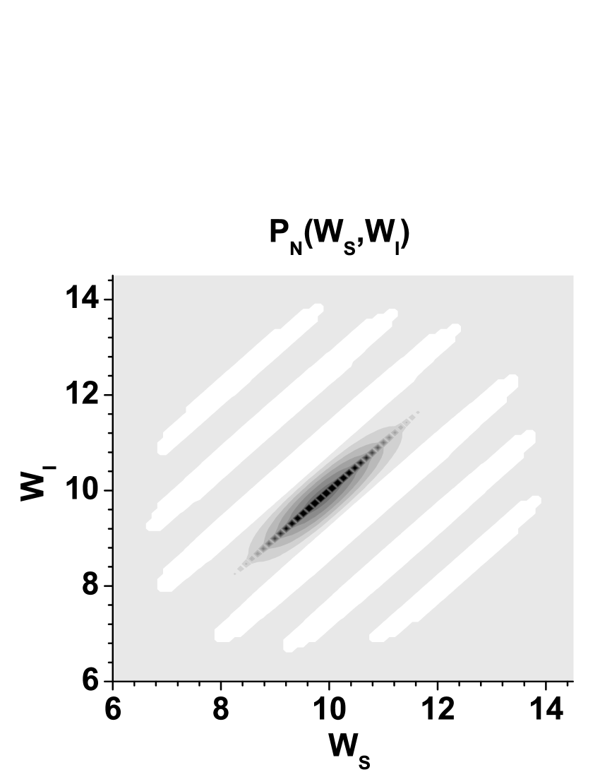
(b)

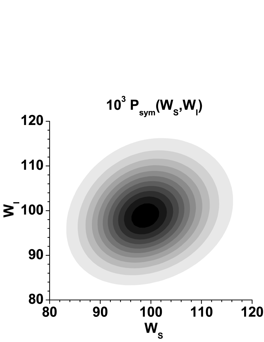
Figure 2: Topo graphs of (a) normally-ordered (${\sf s}=1$) and (b) symmetrically-ordered (${\sf s}=0$) joint SI quasi-distributions $P(W_{s},W_{i})$ of integrated intensities; ${\sf s}_{\rm th}=0.63$. Integrated intensities $W_{s}$ and $W_{i}$ are in units of photon numbers.

III Quasi-distributions of integrated intensities

According to Eq. (1), QDII $P(W_{s},W_{i})$ can be determined as the inverse Fourier transform of the characteristic function $C_{W}$ defined in Eq. (2) (${\sf s}$ means the ordering parameter of field operators Peřina (1991)):

$$P_{\sf s}(W_{s},W_{i}) = \int_{0}^{\infty}dW^{\prime}_{s}\int_{0}^{\infty}dW^{\prime}_{i}P_{p,{\sf s}}(W_{s}-W^{\prime}_{s},W_{i}-W^{\prime}_{i})$$ (17)

$$\mbox{}\times P_{s,{\sf s}}(W^{\prime}_{s})P_{i,{\sf s}}(W^{\prime}_{i}).$$

In Eq. (17), QDII $P_{p,{\sf s}}$ of the field of photon pairs takes the form Peřina and Křepelka (2005):

$$P_{p,{\sf s}}(W_{s},W_{i}) = \frac{({W_{s}W_{i}})^{(M_{p}-1)/2}}{\pi\Gamma(M_{p})B_{p,{\sf s}}^{M_{p}}}\exp\left(-\frac{W_{s}+W_{i}}{2B_{p,{\sf s}}}\right)$$ (18)

$$\mbox{}\times\sqrt{-K_{p,{\sf s}}}{\rm sinc}\left(\frac{W_{s}-W_{i}}{\sqrt{-K_{p,{\sf s}}}}\right),\hskip 14.22636pt{\sf s}>{\sf s}_{\rm th},$$

$$\mbox{}=\;\frac{({W_{s}W_{i}})^{(M_{p}-1)/2}}{\Gamma(M_{p})K_{p,{\sf s}}D_{p}^{M_{p}-1}}\exp\left[-\frac{B_{p,{\sf s}}(W_{s}+W_{i})}{K_{p,{\sf s}}}\right]$$

$$\mbox{}\times{\rm I}_{M_{p}-1}\left(2\frac{D_{p}\sqrt{W_{s}W_{i}}}{K_{p,{\sf s}}}\right),\hskip 14.22636pt{\sf s}<{\sf s}_{\rm th};$$

$B_{p,{\sf s}}=B_{p}+(1-{\sf s})/2$, $D_{p}=\sqrt{B_{p}(B_{p}+1)}$, $K_{p,{\sf s}}=-{\sf s}B_{p}+(1-{\sf s})^{2}/4$ and ${\sf s}_{\rm th}=1+2(B_{p}-\sqrt{B_{p}(B_{p}+1)})$. Symbol $I_{M}$ denotes the modified Bessel function and ${\rm sinc}(x)=\sin(x)/x$. On the other hand, QDIIs $P_{a,{\sf s}}$ of the multi-thermal noise fields occurring in the convolution in Eq. (17) and related to ${\sf s}$ ordering are derived as Peřina (1991):

$$P_{a,{\sf s}}(W_{a})=\frac{W_{a}^{M_{a}-1}}{\Gamma(M_{a})B_{a,{\sf s}}^{M_{a}}}\exp\left(-\frac{W_{a}}{B_{a,{\sf s}}}\right),\hskip 5.69054pta=s,i;$$ (19)

$B_{a,{\sf s}}=B_{a}+(1-{\sf s})/2$. Provided that the noise multi-thermal fields are weak, the QDII $P_{\sf s}$ in Eq. (17) inherits the features of QDII $P_{p,{\sf s}}$ characterizing the field of photon pairs. For the paired field and according to Eq. (18), the QDII $P_{p,{\sf s}}$ maintains its quantum form provided that we are close to the normal-ordering of field operators (${\sf s}>{\sf s}_{\rm th}$). It attains negative values localized in strips parallel to the diagonal due to the pairwise character of the SI field [see Fig. 2(a)]. Faithful description of these strips with negative values requires the introduction of additional independent parameters that complete the five parameters of a general Gaussian form. From this point of view, the separation of fully entangled quantum (paired) part from the rest of the field is extraordinarily convenient as it introduces only one additional independent parameter. For lower values of ordering parameter ${\sf s}$ (${\sf s}<{\sf s}_{\rm th}$), the superimposed detection noise described by the ’ordering of field operators’ conceals negative values and quantum features (entanglement Peřina and Křepelka (2011)) of the SI field. This results in a non-negative QDII $P_{p,{\sf s}}$ with a smoothed shape [see Fig. 2(b)] that can be successfully approximated by a general two-dimensional Gaussian distribution function. In this case, the needed five independent parameters can naturally be determined from the first and second experimental moments. This is usual for any classical field. We note here that a QDII related to any value of ordering operator ${\sf s}_{\rm th}$ can be derived from that related to normal ordering using convolution with an appropriate Gaussian function Peřina (1991). However, this procedure cannot be inverted for principal reasons Peřina (1991). That is why, we need the QDIIs related to normal ordering for full characterization of non-classical states including twin beams.

Considering the general QDII $P_{\sf s}$ in the form of Eq. (17), the threshold value ${\sf s}_{\rm th}$ can be obtained from the analysis of the first and second moments of integrated intensities related to an arbitrary ${\sf s}$ ordering. The condition $\langle[\Delta(W_{s}-W_{i})]^{2}\rangle_{{\sf s}_{\rm th}}=0$ can be rearranged into the formula:

$${\sf s}_{\rm th} = 1+2\left(\beta-\sqrt{\gamma^{2}-\beta}\right),$$ (20)

$$\beta = \frac{M_{s}B_{s}+M_{i}B_{i}+2M_{p}B_{p}}{M_{s}+M_{i}+2M_{p}},$$

$$\gamma = \frac{M_{s}B_{s}^{2}+M_{i}B_{i}^{2}-2M_{p}B_{p}}{M_{s}+M_{i}+2M_{p}}.$$

Inspection of Eq. (15) shows that the threshold value ${\sf s}_{\rm th}$ is below 1 provided that $M_{s}B_{s}^{2}+M_{i}B_{i}^{2}\leq 2M_{p}B_{p}$. This condition for non-classicality of twin beams can be rewritten as

$$\langle(\Delta W_{s})^{2}\rangle+\langle(\Delta W_{i})^{2}\rangle<2\langle W_{p}\rangle.$$ (21)

According to Eq. (21), single-photon noise in the signal and idler fields has to be sufficiently compensated by the paired field to keep non-classicality of twin beams.

Having a joint SI photon-number distribution $p(n_{s},n_{i})$ written in Eq. (7), the distribution $p_{\rm sum}$ of the sum of signal and idler photon numbers with its characteristic teeth-like structure (only even photon-numbers are present) Waks et al. (2004) can easily be obtained [see Fig. 1(b) above]. It provides the simplest experimental evidence of the presence of photon pairs in the analyzed field. The prevailing paired structure of the SI field is also responsible for strong sub-shot-noise correlations in the signal and idler photon-number difference [$\langle(n_{s}-n_{i})^{2}\rangle/(\langle n_{s}\rangle+\langle n_{i}\rangle)=1+\langle(W_{s}-W_{i})^{2}\rangle/(\langle W_{s}\rangle+\langle W_{i}\rangle)=0.07$] Jedrkiewicz et al. (2004); Blanchet et al. (2008); Brida et al. (2009).

IV Conclusions

We have reconstructed a quasi-distribution of integrated intensities of twin beams using the reliable first and second experimental photocount moments and the method of least square declinations. Whereas a general Gaussian form of the quasi-distribution is suitable for a classical field, a more general form is needed for quantum entangled states for which negative values of the quasi-distribution are characteristic. The consideration of quantum-classical transition has revealed a momentum criterion of non-classicality of twin beams. We consider the developed method robust and reliable and as such applicable and prospective also in other areas of quantum physics.