Evolutionary games on the lattice: Payoffs affecting birth and death rates

Abstract

This article investigates an evolutionary game based on the framework of interacting particle systems. Each point of the square lattice is occupied by a player who is characterized by one of two possible strategies and is attributed a payoff based on her strategy, the strategy of her neighbors and a payoff matrix. Following the traditional approach of evolutionary game theory, this payoff is interpreted as a fitness: the dynamics of the system is derived by thinking of positive payoffs as birth rates and the absolute value of negative payoffs as death rates. The nonspatial mean-field approximation obtained under the assumption that the population is well mixing is the popular replicator equation. The main objective is to understand the consequences of the inclusion of local interactions by investigating and comparing the phase diagrams of the spatial and nonspatial models in the four dimensional space of the payoff matrices. Our results indicate that the inclusion of local interactions induces a reduction of the coexistence region of the replicator equation and the presence of a dominant strategy that wins even when starting at arbitrarily low density in the region where the replicator equation displays bistability. We also discuss the implications of these results in the parameter regions that correspond to the most popular games: the prisoner’s dilemma, the stag hunt game, the hawk-dove game and the battle of the sexes.

T1Supported in part by NSF Grant DMS-10-05282.

1 Introduction

The book of von Neumann and Morgenstern vonneumann_morgenstern_1944 that develops mathematical methods to understand human behavior in strategic and economic decisions is the first foundational work in the field of game theory. The most popular games are symmetric two-person games whose characteristics are specified by a square matrix where the common number of rows and columns denotes the number of possible pure strategies, and the coefficients represent the player’s payoffs which depend on both her strategy and the strategy of her opponent. Game theory relies on the assumption that players are rational decision-makers. In particular, the main question in this field is: what is the best possible response against a player who tries to maximize her payoff? The work of Nash nash_1950 on the existence of Nash equilibrium, a mathematical criterion for mutual consistency of players’ strategies, is an important contribution that gives a partial answer to this question.

In contrast, the field of evolutionary game theory, which was proposed by theoretical biologist Maynard Smith and first appeared in his work with Price maynardsmith_price_1973 , does not assume that players make rational decisions: evolutionary game theory makes use of concepts from traditional game theory to describe the dynamics of populations by thinking of individuals as interacting players and their trait as a strategy, and by interpreting their payoff as a fitness or reproduction success. The analog of Nash equilibrium in evolutionary game theory is called ESS, a short for evolutionary stable strategy, and is defined as a strategy which, if adopted by a population, cannot be invaded by any alternative strategy starting at an infinitesimally small frequency. This key concept first appeared in the foundational work maynardsmith_price_1973 . Even though evolutionary games were originally introduced to understand the outcome of animal conflicts, they now have a wide variety of applications as a powerful framework to study interacting populations in which the reproductive success of each individual is density dependent, a key component of social and biological communities.

The inclusion of stochasticity and space in the form of local interactions is another key factor in how communities are shaped, and evolutionary games have been studied through both the mathematical analysis of deterministic nonspatial models based on differential equations and simulations of more complex models based on spatial stochastic processes. For a review on deterministic nonspatial evolutionary games, we refer to hofbauer_sigmund_1998 . On the side of spatial stochastic evolutionary games, one important contribution is the work of Nowak and May nowak_may_1992 , nowak_may_1993 which, based on simulations of cellular automata, shows that space favors cooperation in the prisoner’s dilemma. See also nowak_bonhoeffer_may_1994a , nowak_bonhoeffer_may_1994b for similar works based on asynchronous updating models, nowak_2006 for a review on spatial evolutionary games and fu_nowak_hauert_2010 , langer_nowak_hauert_2010 and references therein for more recent work on the topic. The rigorous analysis of nonspatial deterministic models and simulations of spatial stochastic models are both important and complementary but also have some limitations: spatial simulations suggest that nonspatial models fail to appropriately describe systems, including local interactions, but are known at the same time to be difficult to interpret, leading sometimes to erroneous conclusions. This underlines the necessity of an analytical study of evolutionary games based on stochastic spatial models. References chen_2013 , cox_durrett_perkins_2013 , durrett_2013 are, as far as we know, the only three articles that also carry out a rigorous analysis of such models but the authors’ approach significantly differs from ours: they assume that

$$\mbox{fitness}=(1-w)+w\times\mbox{payoff}\quad\mbox{and}\quad w\to 0,$$

which is referred to as weak selection and allows for a complete analytical treatment using voter model perturbation techniques. Indeed, for $w=0$, their model reduces to the popular voter model introduced in clifford_sudbury_1973 , holley_liggett_1975 . In contrast, we assume that fitness${}={}$payoff, which makes our model mathematically more challenging and does not allow for a complete analysis. However, the limiting behavior in different parameter regions can be understood based on various techniques, which leads to interesting findings about the consequences of the inclusion of local interactions. For a similar approach, we also refer to evilsizor_lanchier_2014 where the best-response dynamics, a spatial process in which players update their strategy at a constant rate in order to maximize their payoff, is studied.

The replicator equation

As previously mentioned, most of the analytical works in evolutionary game theory are based on ordinary differential equations. The most popular model that falls into this category is the replicator equation, which we describe for simplicity in the presence of only two strategies since this is the case under consideration for the stochastic spatial model we introduce later. The dynamics depends on a $2\times 2$ payoff matrix $A=(a_{ij})$ where $a_{ij}$ denotes the payoff of a player who follows strategy $i$ interacting with a player who follows strategy $j$. To formulate the replicator equation and describe its bifurcation diagram, it is convenient to use the terminology introduced by the author in lanchier_2012 by setting

$$a_{1}:=a_{11}-a_{21}\quad\mbox{and}\quad a_{2}:=a_{22}-a_{12}$$

and declaring strategy $i$ to be:

• altruistic when $a_{i}<0$, that is, a player with strategy $i$ confers a lower payoff to a player following the same strategy than to a player following the other strategy,

• selfish when $a_{i}>0$, that is, a player with strategy $i$ confers a higher payoff to a player following the same strategy than to a player following the other strategy.

The replicator equation is a system of coupled differential equations for the frequency $u_{i}$ of players following strategy $i$. The payoff of each type $i$ player is given by

$$\phi_{i}=\phi_{i}(u_{1},u_{2}):=a_{i1}u_{1}+a_{i2}u_{2}\qquad\mbox{for }i=1,2.$$ (1)

Interpreting this payoff as the growth rate of each type $i$ player, using that the frequencies sum up to one, and recalling the definition of $a_{1}$ and $a_{2}$, one obtains the following ordinary differential equation, the so-called replicator equation, for the frequency of type 1 players:

$$u_{1}^{\prime}(t) = u_{1}u_{2}(\phi_{1}-\phi_{2})=u_{1}u_{2}(a_{11}u_{1}+a_{12}u_{2}-a_{21}u_{1}-a_{22}u_{2})$$

$$= u_{1}u_{2}(a_{1}u_{1}-a_{2}u_{2})=u_{1}(1-u_{1})\bigl{(}(a_{1}+a_{2})u_{1}-a_{2}\bigr{)}.$$

The system has three fixed points, namely

$$e_{1}:=1\quad\mbox{and}\quad e_{2}:=0\quad\mbox{and}\quad e_{12}:=a_{2}(a_{1}+a_{2})^{-1},$$

and basic algebra shows that the limiting behavior only depends on the sign of $a_{1}$ and $a_{2}$, therefore on whether strategies are altruistic or selfish. More precisely, we find that:

• when strategy 1 is selfish and strategy 2 altruistic, strategy 1 wins: $e_{12}\notin(0,1)$ and starting from any initial condition $u_{1}(0)\in(0,1)$, $u_{1}\to e_{1}$.

• when strategy 1 is altruistic and strategy 2 selfish, strategy 2 wins: $e_{12}\notin(0,1)$ and starting from any initial condition $u_{1}(0)\in(0,1)$, $u_{1}\to e_{2}$.

• when both strategies are altruistic, coexistence occurs: $e_{12}\in(0,1)$ is globally stable, that is, starting from any initial condition $u_{1}(0)\in(0,1)$, $u_{1}\to e_{12}$.

• when both strategies are selfish, the system is bistable: $e_{12}\in(0,1)$ is unstable, and $u_{1}$ converges to either $e_{1}$ or $e_{2}$ depending on whether it is initially larger or smaller than $e_{12}$.

In terms of evolutionary stable strategy, this indicates that, for well-mixed populations, a strategy is evolutionary stable if it is selfish, but not if it is altruistic.

Spatial analog

To define a spatial analog of the replicator equation, we employ the framework of interacting particle systems by positioning the players on an infinite grid. Our spatial game is then described by a continuous-time Markov chain $\eta_{t}$ whose state space maps the $d$-dimensional lattice into the set of strategies $\{1,2\}$, with $\eta_{t}(x)$ denoting the strategy at vertex $x$. Players being located on a geometrical structure, space can be included in the form of local interactions by assuming that the payoff of each player is computed based on the strategy of her neighbors. More precisely, we define the interaction neighborhood of vertex $x$ as

$$N_{x}:=\Bigl{\{}y\in\mathbb{Z}^{d}\dvtx y\neq x\mbox{ and }\max_{i=1,2,\ldots,d}|y_{i}-x_{i}|\leq M\Bigr{\}}\qquad\mbox{for }x\in\mathbb{Z}^{d},$$

where $M$ is referred to as the dispersal range. Letting $f_{j}(x,\eta)$ denote the fraction of type $j$ players in the neighborhood of vertex $x$, the payoff of $x$ is then defined as

$$\phi\bigl{(}x,\eta|\eta(x)=i\bigr{)}:=a_{i1}f_{1}(x,\eta)+a_{i2}f_{2}(x,\eta)\qquad\mbox{for }i=1,2,$$

which can be viewed as the spatial analog of (1). The dynamics is again derived by interpreting the payoff as a fitness. More precisely, we think of a payoff as either a birth rate or a death rate depending on its sign: if the player at vertex $x$ has a positive payoff, then at rate this payoff, one of her neighbors chosen uniformly at random adopts the strategy at $x$, while if she has a negative payoff, then at rate minus this payoff, she adopts the strategy of one of her neighbors again chosen uniformly at random. This is described formally by the Markov generator

$$Lf(\eta)$$

$$\qquad=N^{-1}\sum_{x}\sum_{y\in N_{x}}\phi(y,\eta)\mathbf{1}\bigl{\{}\phi(y,\eta)>0\bigr{\}}\mathbf{1}\bigl{\{}\eta(x)\neq\eta(y)\bigr{\}}\bigl{[}f(\eta_{x})-f(\eta)\bigr{]}$$ (3)

$$\qquad\quad{}-N^{-1}\sum_{x}\sum_{y\in N_{x}}\phi(x,\eta)\mathbf{1}\bigl{\{}\phi(x,\eta)<0\bigr{\}}\mathbf{1}\bigl{\{}\eta(x)\neq\eta(y)\bigr{\}}\bigl{[}f(\eta_{x})-f(\eta)\bigr{]},$$

where configuration $\eta_{x}$ is obtained from configuration $\eta$ by changing the strategy at vertex $x$ and leaving the strategy at the other vertices unchanged, and where the constant $N$ is simply the common size of the interaction neighborhoods. Note that $L$ indeed defines a unique Markov process according to, for example, Theorem B3 in Liggett liggett_1999 . Model (1) is inspired from the spatial version of Maynard Smith’s evolutionary games introduced by Brown and Hansell brown_hansell_1987 . Their model allows for any number of players per vertex, and the dynamics includes three components: migration, death due to crowding and birth or death based on the value of the payoff. Our model only retains the third component. We also point out that the model obtained from (1) by assuming that the population is well mixing, called the mean-field approximation, is precisely the replicator equation (1). Therefore the consequences of the inclusion of space and stochasticity can indeed be understood through the comparison of both models, which as we show later, disagree in many ways. In fact, the original model of Brown and Hansell is also studied numerically in durrett_levin_1994 where it is used to argue that the inclusion of space and/or stochasticity can lead to drastic behavior changes.

Main results

We now study the limiting behavior of the spatial game. Unless explicitly stated otherwise, all the results below apply to the process starting from Bernoulli product measures in which the density of each strategy is positive and constant across space:

$$P\bigl{(}\eta_{0}(x_{1})=\eta_{0}(x_{2})=\cdots=\eta_{0}(x_{n})=1\bigr{)}=\rho^{n}\qquad\mbox{for some }\rho\in(0,1)$$ (4)

and every finite sequence $x_{1},x_{2},\ldots,x_{n}$ of distinct vertices. From the point of view of the replicator equation, whether a strategy wins, or both strategies coexist or the system is bistable is defined based on the value of the nontrivial fixed point $e_{12}$ and the stability of this and the other two fixed points. For the spatial game, we say that:

• strategy $i\in\{1,2\}$ survives whenever

  $$P\bigl{(}\eta_{s}(x)=i\mbox{ for some }s>t\bigr{)}=1\qquad\mbox{for all }(x,t)\in\mathbb{Z}^{d}\times\mathbb{R}_{+};$$

• strategy $i\in\{1,2\}$ goes extinct whenever

  $$\lim_{t\to\infty}P\bigl{(}\eta_{t}(x)=i\bigr{)}=0\qquad\mbox{for all }x\in\mathbb{Z}^{d};$$

• a strategy wins if it survives whereas the other strategy goes extinct;

• both strategies coexist whenever

  $$\liminf_{t\to\infty}P\bigl{(}\eta_{t}(x)\neq\eta_{t}(y)\bigr{)}>0\qquad\mbox{for all }x,y\in\mathbb{Z}^{d};$$

• the system clusters whenever

  $$\lim_{t\to\infty}P\bigl{(}\eta_{t}(x)\neq\eta_{t}(y)\bigr{)}=0\qquad\mbox{for all }x,y\in\mathbb{Z}^{d}.$$

Numerical simulations suggest that in the presence of one selfish and one altruistic strategy, the selfish strategy wins, just as in the replicator equation. In contrast, when both strategies are selfish, spatial and nonspatial models disagree. Our brief analysis of the replicator equation indicates that the system is bistable: both strategies are ESS. The transition curve for the spatial model is difficult to find based on simulations, but simple heuristic arguments looking at the interface between two adjacent blocks of the two strategies suggest that the most selfish strategy, that is, the one with the largest $a_{i}$, always wins even when starting at a very low density, thus indicating that only the most selfish strategy is an ESS. The fact that bistability in the mean-field model results in the presence of a strong type in the interacting particle system has already been observed for a number of models, and we refer to durrett_2009 , durrett_levin_1994 for such examples. For two altruistic strategies, coexistence is again possible, but the coexistence region of the spatial game is significantly smaller than that of the replicator equation: except in the one-dimensional nearest neighbor case, coexistence occurs in a thorn-shaped region starting at the bifurcation point $a_{1}=a_{2}=0$. The smaller the range of the interactions and the spatial dimension, the smaller the coexistence region. In the one-dimensional nearest neighbor case, the simulations are particularly difficult to interpret when

$$a_{11}+a_{12}<0<a_{12}\quad\mbox{and}\quad a_{22}+a_{21}<0<a_{21}.$$ (5)

See Figure 4 for a picture of two realizations when (5) holds. However, we were able to prove that the one-dimensional nearest neighbor system clusters except in a parameter region with measure zero in the space of the $2\times 2$ matrices in which all the players have a zero payoff eventually, thus leading to a fixation of the system in a configuration in which both strategies are present. More generally, we conjecture that, except in this parameter region with measure zero, the least altruistic strategy always wins, just as in the presence of selfish-selfish interactions. The thick continuous lines on the right-hand side of Figures 1 and 2 summarize our conjectures for the spatial game in the one-dimensional nearest neighbor case and all the other cases, respectively. These results are reminiscent of the ones obtained for the models introduced in lanchier_2012 , lanchier_neuhauser_2009 , neuhauser_pacala_1999 , which though they are not examples of evolutionary games, also include density-dependent birth or death rates. Our proofs and the proofs in these three references strongly differ while showing the same pattern: for all four models, the inclusion of local interactions induces a reduction of the coexistence region of the mean-field model, and there is a dominant type that wins even when starting at arbitrarily low density in the region where the mean-field model displays bistability.

We now state our analytical results for the spatial stochastic process, which confirms in particular these two important aspects. To motivate and explain our first result, we observe that the presence of density-dependent birth and death rates typically precludes the existence of a mathematically tractable dual process. See Liggett liggett_1985 , Section II.3, for a general definition of duality and dual process. Note, however, that if $a_{11}=a_{12}$ and $a_{22}=a_{21}$, then the payoff of players of either type is constant across all possible spatial configurations: birth and death rates are no longer density dependent. For this specific choice of the payoffs, the process reduces to a biased voter model bramson_griffeath_1980 , bramson_griffeath_1981 , and therefore strategy 1 wins if in addition $a_{12}>a_{21}$. For all other payoff matrices, the dynamics is more complicated, but there is a large parameter region in which the spatial game can still be coupled with a biased voter model to deduce that strategy 1 wins. This parameter region is specified in the following theorem. See also the right-hand side of Figure 2 where the boundary of this region is represented in dashed lines on the $a_{11}-a_{22}$ plane.

Theorem 1

Assume that $a_{12}>a_{21}$. Then strategy 1 wins whenever

$$\max(a_{22},a_{21})+a_{21}(N-1)^{-1}<\min(a_{11},a_{12})+a_{12}(N-1)^{-1}.$$

This parameter region intersects the regions in which the replicator equation displays coexistence and bistability. In particular, the theorem confirms that the inclusion of local interactions induces a reduction of the coexistence and bistable regions in accordance with the simulation results mentioned above. The next two results strengthen this theorem by proving that the parameter region in which there is a unique ESS extends to arbitrarily small/large values of $a_{11}$ and $a_{22}$. To state these results, it is convenient to introduce the vector $\bar{a}_{11}:=(a_{12},a_{21},a_{22})$.

Theorem 2

For all $\bar{a}_{11}$ there exists $m(\bar{a}_{11})<\infty$ such that

$$\mbox{strategy 1 wins whenever }a_{11}>m(\bar{a}_{11}).$$

This implies that, in accordance with our numerical simulations, the parameter region in which the replicator equation is bistable while there is a unique ESS for the spatial game is much larger than the parameter region covered by Theorem 1. Note also that, in view of the symmetry of the model, the previous theorem also holds by exchanging the roles of the two strategies.

Theorem 3

For all $\bar{a}_{11}$ such that $a_{12}<0$, there exists $m(\bar{a}_{11})<\infty$ such that

$$\mbox{strategy 2 wins whenever }a_{11}<-m(\bar{a}_{11}).$$

This implies that, again in accordance with our numerical simulations, the parameter region in which coexistence occurs for the replicator equation while there is a unique ESS for the spatial game is much larger than the one covered by Theorem 1. Once more, we point out that, in view of the symmetry of the model, the theorem also holds by exchanging the roles of the two strategies as indicated in Figure 2. The previous two results hold regardless of the spatial dimension and the range of the interactions and can be significantly improved in the one-dimensional nearest neighbor case through an analysis of the boundaries of the system. More precisely, letting

$$\mathcal{M}_{2}^{*} := \bigl{\{}A=(a_{ij})\mbox{ such that}$$

$$\hskip 6.0pta_{11}a_{12}a_{21}a_{22}(a_{11}+a_{12})(a_{22}+a_{21})\neq 0\mbox{ and }a_{11}+a_{12}\neq a_{22}+a_{21}\bigr{\}}$$

we have the following theorem.

Theorem 4

Assume that $M=d=1$. Then:

• strategy 1 wins for all $a_{11}>\max(a_{22},a_{21})+(a_{21}-a_{12})$, and

• the system starting from any translation invariant distribution clusters for all $A\in\mathcal{M}_{2}^{*}$.

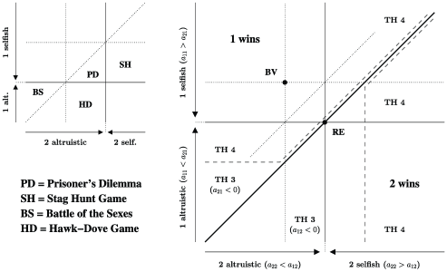
Figure 1: List of the most popular $2\times 2$ games on the left and phase diagrams of the spatial game along with a summary of the theorems in the $a_{11}-a_{22}$ plane on the right. The thick lines refer to the transition curves suggested by the simulations. BV${}={}$biased voter model, and RE${}={}$replicator equation.

Figure 1 gives the phase diagram of the one-dimensional nearest neighbor process obtained by combining Theorems 3 and 4. The parameter region in the first part of Theorem 4, and the one obtained by symmetry are represented in dashed lines when $a_{12}>a_{21}$. For most of the parameter region in which at least one strategy is selfish, the most selfish strategy wins, which significantly improves Theorem 2. The second part of the theorem supplements Theorem 3 by proving that, except in the measure zero parameter region that corresponds to $A\in\mathcal{M}_{2}^{*}$, coexistence is not possible in the one-dimensional nearest neighbor case. Finally, our last theorem looks more closely at the interactions between two altruistic strategies and confirms that, except in the one-dimensional nearest neighbor case, coexistence is possible for the spatial game.

Theorem 5

There is $m:=m(a_{12},a_{21})>0$ such that coexistence occurs when

$$c(M,d)a_{22}<a_{11}<-m\quad\mbox{and}\quad c(M,d)a_{11}<a_{22}<-m,$$

where, for each range $M$ and spatial dimension $d$,

$$c(M,d):=\frac{2M((2M+1)^{d}-2)}{(M+1)(2M(2M+1)^{d-1}-1)}.$$

Note that the parameter region in the theorem is nonempty if and only if $c(M,d)$ is strictly larger than one. In addition, the larger $c(M,d)$, the larger this parameter region. This, together with Table 1, indicates that, except in the one-dimensional nearest neighbor case in which the region given in the theorem is empty, the coexistence region contains an infinite subset of a certain triangle whose range increases with both the dispersal range and the spatial dimension. We refer to Figure 2 for a summary of the theorems that exclude the one-dimensional nearest neighbor case.

Table 1: $c(M,d)$ for different values of the range $M$ and the dimension $d$

	$\bolds{d=1}$	$\bolds{d=2}$	$\bolds{d=3}$	$\bolds{d=4}$	$\bolds{d=5}$	$\bolds{d=6}$	$\bolds{d=7}$	$\bolds{d=8}$	$\bolds{d=9}$
$M=1$	1.0000	1.4000	1.4706	1.4906	1.4969	1.4990	1.4997	1.4999	1.5000
$M=2$	1.3333	1.6140	1.6566	1.6647	1.6663	1.6666	1.6667	1.6667	1.6667
$M=3$	1.5000	1.7195	1.7457	1.7494	1.7499	1.7500	1.7500	1.7500	1.7500
$M=4$	1.6000	1.7803	1.7978	1.7998	1.8000	1.8000	1.8000	1.8000	1.8000
$M=5$	1.6667	1.8196	1.8321	1.8332	1.8333	1.8333	1.8333	1.8333	1.8333
$M=6$	1.7143	1.8470	1.8564	1.8571	1.8571	1.8571	1.8571	1.8571	1.8571
$M=7$	1.7500	1.8672	1.8745	1.8750	1.8750	1.8750	1.8750	1.8750	1.8750
$M=8$	1.7778	1.8827	1.8885	1.8889	1.8889	1.8889	1.8889	1.8889	1.8889
$M=9$	1.8000	1.8950	1.8997	1.9000	1.9000	1.9000	1.9000	1.9000	1.9000

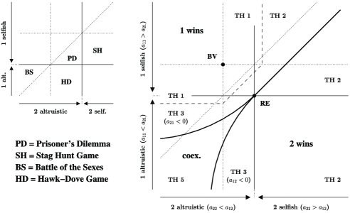
Figure 2: List of the most popular $2\times 2$ games on the left and phase diagrams of the spatial game along with a summary of the theorems in the $a_{11}-a_{22}$ plane on the right. The thick lines refer to the transition curves suggested by the simulations. BV${}={}$biased voter model, and RE${}={}$replicator equation.

The role of space in the most popular games

The last step before going into the details of the proofs is to discuss the implications of our results in the most popular symmetric two-person games. To define these games, note that there are $4!=24$ possible orderings of the four payoffs therefore, also accounting for symmetry, twelve possible strategic situations corresponding to twelve symmetric two-person games involving two strategies. These twelve regions of the parameter space are represented in the $a_{11}-a_{22}$ plane on the left-hand diagrams of Figures 1–2 along with the names of the most popular games under the assumption $a_{12}>a_{21}$.

Prisoner’s dilemma. The prisoner’s dilemma is probably the most popular symmetric two-person game. When $a_{12}>a_{21}$, strategy 1 means defection whereas strategy 2 means cooperation. From the point of view of the replicator equation, defection is the only ESS. Numerical simulations suggest that the same holds for our spatial model, which is covered in part in the general case and completely in the one-dimensional nearest neighbor case in Theorems 1 and 4.

Stag hunt. In the stag hunt game with $a_{12}>a_{21}$, strategy 1 represents safety: hunting a hare, whereas strategy 2 represents social cooperation: hunting a stag. In the absence of space, both strategies are evolutionary stable. In contrast, Theorem 2 shows that, in the presence of local interactions, social cooperation is the only ESS if the reward $a_{22}$ for social cooperation is high enough, that is, a stag is worth much more than a hare, whereas if the reward is not significant, then safety becomes the only ESS according to Theorems 1 and 4.

Hawk-dove. In the hawk-dove game, strategy 1 represents hawks that fight for the resource and strategy 2, doves that share peacefully the resource. The cost of a fight is larger than the value of the contested resource, which makes this game an example of anti-coordination game: the best possible response to a strategy is to play the other strategy. In the absence of space, none of the strategies is evolutionary stable so coexistence occurs. In contrast, Theorem 3 indicates that, in the presence of a spatial structure, the dove strategy is the only ESS when the cost of an escalated fight is high enough or equivalently when $a_{11}$ is small enough.

Battle of the sexes. In the battle of the sexes, husband and wife cannot remember if they planned to meet at the opera or at the football match. The husband would prefer the match and the wife the opera, but overall both would prefer to go to the same place. Mutual cooperation, that is, both go to the place that the other prefers, leads to the lowest possible payoff $a_{22}$ which makes this game another example of anti-coordination game. In the absence of space, none of the strategies is evolutionary stable, so coexistence occurs. Coexistence is also possible in the presence of a spatial structure according to Theorem 5. However, if the cost of mutual cooperation is too high, that is, $a_{22}$ too small, then defection becomes the unique ESS according to Theorem 3.

The rest of the paper is devoted to the proofs of the theorems. We point out that the theorems are not proved in the order they are stated but instead grouped based on the approach and techniques they rely on, which makes the reading of the proofs somewhat easier.

2 Proof of Theorem 4

We first study the one-dimensional nearest neighbor system. The analysis in this case relies on the study of the process that keeps track of the boundaries between the two strategies and strongly differs from the analysis of the system in higher spatial dimensions or with a larger range of interactions. Throughout this section, we let $\xi_{t}$ denote the boundary process

$$\xi_{t}(x):=\eta_{t}(x+1/2)-\eta_{t}(x-1/2)\qquad\mbox{for all }x\in\mathbb{D}:=\mathbb{Z}+1/2$$

and think of sites in state 0 as empty, sites in state $+1$ as occupied by a $+$ particle and sites in state $-1$ as occupied by a $-$ particle. To begin with, we assume that

$$\eta_{0}\dvtx\mathbb{Z}\longrightarrow\{1,2\}\qquad\mbox{is such that }\eta_{0}(x)=1\mbox{ for all }x\leq M,$$ (7)

where $M$ is a positive integer. Note that, from the point of view of the boundary process, this implies that we start with no particle to the left of $M$. Also, we let

$$X_{t}:=\inf\bigl{\{}x\in\mathbb{D}\dvtx\xi_{t}(x)\neq 0\bigr{\}}=\inf\bigl{\{}x\in\mathbb{D}\dvtx\xi_{t}(x)=1\bigr{\}}$$

denote the position of the leftmost particle, which is necessarily a $+$ particle in view of the initial configuration. The key to proving the first part of Theorem 4 is given by the next lemma, which shows the result when starting from the particular initial configuration (7).

Lemma 6.

Assume (7) and $a_{11}>\max(a_{22},a_{21})+(a_{21}-a_{12})$. Then

$$P\Bigl{(}X_{t}>0\mbox{ for all }t>0\mbox{ and }\lim_{t\to\infty}X_{t}=\infty\Bigr{)}\geq 1-\exp(-a_{0}M)$$

$$\eqntext{\mbox{for some }a_{0}>0.}$$ (8)

The idea is to prove that there exists $a>0$ such that

$$\lim_{h\to 0}h^{-1}E(Z_{t+h}-Z_{t}|Z_{t})\leq 0\qquad\mbox{almost surely }\mbox{where }Z_{t}:=\exp(-aX_{t})$$

and then apply the optimal stopping theorem to the supermartingale $(Z_{t})$. Since the transition rates of the process $(X_{t})$ depends on the distance between the $+$ particle it keeps track of and the next particle to the right, we introduce the gap process

$$K_{t} := \inf\bigl{\{}x\in\mathbb{D}\dvtx x>X_{t}\mbox{ and }\xi_{t}(x)\neq 0\bigr{\}}-X_{t}$$

$$= \inf\bigl{\{}x\in\mathbb{D}\dvtx x>X_{t}\mbox{ and }\xi_{t}(x)=-1\bigr{\}}-X_{t}.$$

Looking at the payoff of the players at sites $X_{t}\pm 1/2$ and their associated birth and death rates, which are reported in Figure 3 depending on the value of the gap, we find

$$\Phi_{1}(a) := \lim_{h\to 0}h^{-1}E(Z_{t+h}-Z_{t}|Z_{t},K_{t}=1)$$

$$\leq \bigl{(}e^{-a(X_{t}+2)}-e^{-aX_{t}}\bigr{)}\lim_{h\to 0}h^{-1}P(X_{t+h}-X_{t}\geq 2|K_{t}=1)$$

$${}+\bigl{(}e^{-a(X_{t}-1)}-e^{-aX_{t}}\bigr{)}\lim_{h\to 0}h^{-1}P(X_{t+h}-X_{t}=-1|K_{t}=1)$$

$$= Z_{t}\bigl{(}e^{-2a}-1\bigr{)}\bigl{(}(1/4)\max(0,a_{11}+a_{12})+\max(0,-a_{21})\bigr{)}$$

$${}+Z_{t}\bigl{(}e^{a}-1\bigr{)}\bigl{(}(1/4)\max(0,-a_{11}-a_{12})+(1/2)\max(0,a_{21})\bigr{)}$$

$$=: \Psi_{1}(a)$$

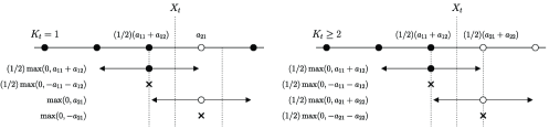
Figure 3: Picture related to the proof of Lemma 6. The numbers are the top of both pictures are the payoffs of the two players at $X_{t}\pm 1/2$ and the numbers at the bottom the associated birth and death rates. Birth events are symbolically represented by double arrows and death events by crosses.

almost surely, where the inequality is obtained by ignoring births from $X_{t}+3/2$ and jumps of more than two units to the right. Note also that the derivative of the right-hand side evaluated at $a=0$ satisfies the following inequality almost surely:

$$\Psi^{\prime}_{1}(0) = -(1/2)\max(0,a_{11}+a_{12})Z_{t}-2\max(0,-a_{21})Z_{t}$$

$${}+(1/4)\max(0,-a_{11}-a_{12})Z_{t}+(1/2)\max(0,a_{21})Z_{t}$$

$$\leq (1/4)\max(0,-a_{11}-a_{12})Z_{t}-(1/4)\max(0,a_{11}+a_{12})Z_{t}$$

$${}+(1/2)\max(0,a_{21})Z_{t}-(1/2)\max(0,-a_{21})Z_{t}$$

$$= (1/4)(-a_{11}-a_{12}+2a_{21})Z_{t}$$

$$\leq (1/4)\bigl{(}\max(a_{22},a_{21})+(a_{21}-a_{12})-a_{11}\bigr{)}Z_{t}<0.$$

Similarly, conditioning on the event $K_{t}\geq 2$, we have

$$\Phi_{2}(a) := \lim_{h\to 0}h^{-1}E(Z_{t+h}-Z_{t}|Z_{t},K_{t}\geq 2)$$

$$= \bigl{(}e^{-a(X_{t}+1)}-e^{-aX_{t}}\bigr{)}\lim_{h\to 0}h^{-1}P(X_{t+h}-X_{t}=1|K_{t}\geq 2)$$

$${}+\bigl{(}e^{-a(X_{t}-1)}-e^{-aX_{t}}\bigr{)}\lim_{h\to 0}h^{-1}P(X_{t+h}-X_{t}=-1|K_{t}\geq 2)$$

$$= Z_{t}\bigl{(}e^{-a}-1\bigr{)}(1/4)\bigl{(}\max(0,a_{11}+a_{12})+\max(0,-a_{22}-a_{21})\bigr{)}$$

$$+Z_{t}\bigl{(}e^{a}-1\bigr{)}(1/4)\bigl{(}\max(0,-a_{11}-a_{12})+\max(0,a_{22}+a_{21})\bigr{)}$$

almost surely. Taking again the derivative at $a=0$, we get

$$\Phi^{\prime}_{2}(0) = -(1/4)\max(0,a_{11}+a_{12})Z_{t}-(1/4)\max(0,-a_{22}-a_{21})Z_{t}$$

$${}+(1/4)\max(0,-a_{11}-a_{12})Z_{t}+(1/4)\max(0,a_{22}+a_{21})Z_{t}$$

$$= (1/4)(-a_{11}-a_{12}+a_{22}+a_{21})Z_{t}$$

$$\leq (1/4)\bigl{(}\max(a_{22},a_{21})+(a_{21}-a_{12})-a_{11}\bigr{)}Z_{t}<0$$

almost surely. From (2)–(2), we deduce that

$$\Phi_{1}(a_{0})\leq\Psi_{1}(a_{0})\leq\Psi_{1}(0)=0\quad\mbox{and}\quad\Phi_{2}(a_{0})\leq\Phi_{2}(0)=0$$

for some $a_{0}>0$ fixed from now on. In particular,

$$\lim_{h\to 0}h^{-1}E\bigl{(}\exp(-a_{0}X_{t+h})-\exp(-a_{0}X_{t})|X_{t}\bigr{)}\leq 0\qquad\mbox{almost surely},$$

which shows that $Z_{t}=\exp(-a_{0}X_{t})$ is a supermartingale. As mentioned above, we conclude using the optimal stopping theorem: we introduce the stopping times

$$\tau_{-}:=\inf\{t\dvtx X_{t}=-1/2\}\quad\mbox{and}\quad\tau_{n}:=\inf\{t\dvtx X_{t}\geq n+1/2\}\qquad\mbox{for all }n>M.$$

Using that $T_{n}:=\min(\tau_{-},\tau_{n})$ is almost surely finite, we get

$$EZ_{T_{n}} \leq EZ_{0}=Ee^{-a_{0}X_{0}}\leq e^{-a_{0}M},$$

$$EZ_{T_{n}} = E(Z_{T_{n}}|T_{n}=\tau_{-})P(T_{n}=\tau_{-})+E(Z_{T_{n}}|T_{n}=\tau_{n})P(T_{n}=\tau_{n})$$

$$\geq e^{a_{0}/2}\bigl{(}1-P(T_{n}=\tau_{n})\bigr{)}+e^{-a_{0}n}P(T_{n}=\tau_{n}).$$

Observing that the sequence $\{T_{n}=\tau_{n}\}$ is nonincreasing for the inclusion, applying the monotone convergence theorem and using the previous inequalities, we deduce that

$$P\Bigl{(}X_{t}>0\mbox{ for all }t>0\mbox{ and }\lim_{t\to\infty}X_{t}=\infty\Bigr{)}$$

$$\qquad\geq P(T_{n}=\tau_{n}\mbox{ for all }n>M)=\lim_{n\to\infty}P(T_{n}=\tau_{n})$$

$$\qquad\geq\lim_{n\to\infty}\bigl{(}e^{a_{0}/2}-e^{-a_{0}M}\bigr{)}\bigl{(}e^{a_{0}/2}-e^{-a_{0}n}\bigr{)}^{-1}\geq 1-e^{-a_{0}M}.$$

This completes the proof of the lemma.

It follows from the previous lemma that, starting more generally from a product measure with a positive density of type 1 players, strategy 1 wins with probability one. This statement, which corresponds to the first part of Theorem 4, is proved in the next lemma.

Lemma 7.

Assume (4) and $a_{11}>\max(a_{22},a_{21})+(a_{21}-a_{12})$. Then strategy 1 wins.

Let $M$ be a positive integer, and let

$$x_{M}:=\inf\bigl{\{}x\in\mathbb{Z}\dvtx x>0\mbox{ and }\eta_{0}(x)=\eta_{0}(x+1)=\cdots=\eta_{0}(x+2M+2)=1\bigr{\}}.$$

Note that, starting from (4), vertex $x_{M}$ is well defined and almost surely finite. We define the cluster starting at $x_{M}$ as the set of space–time points that can be reached from $x_{M}$ by a path moving forward in time and contained in the space–time region occupied by type 1 players

$$C(x_{M}):=\bigl{\{}(x,t)\in\mathbb{Z}\times\mathbb{R}_{+}\dvtx(x_{M},0)\to(x,t)\bigr{\}},$$

where $(x_{M},0)\to(x,t)$ means that there exist

$$z_{0}=x_{M},z_{1},\ldots,z_{n}:=x\in\mathbb{Z}\quad\mbox{and}\quad s_{0}:=0<s_{1}<\cdots<s_{n}<s_{n+1}:=t\in\mathbb{R}_{+}$$

such that the following two conditions hold:

• for $i=1,2,\ldots,n$, we have $|z_{i}-z_{i-1}|=1$, and

• for $i=0,1,\ldots,n$, we have $\eta_{s}(x_{i})=1$ for all $s_{i}\leq s\leq s_{i+1}$.

Finally, for all times $t$, we let

$$l_{t}:=\inf\bigl{\{}x\in\mathbb{Z}\dvtx(x,t)\in C(x_{M})\bigr{\}}\quad\mbox{and}\quad r_{t}:=\sup\bigl{\{}x\in\mathbb{Z}\dvtx(x,t)\in C(x_{M})\bigr{\}}$$

be, respectively, the leftmost and the rightmost vertices in the cluster. Due to one-dimensional nearest neighbor interactions, as long as the cluster is nonempty, all vertices between the leftmost and rightmost vertices follow strategy 1. In particular, it follows from Lemma 6 and the obvious symmetry of the evolution rules that the probability that strategy 1 wins is larger than

$$P\bigl{(}(x,t)\in C(x_{M})\mbox{ for all $x\in\mathbb{Z}$ and all $t$ large}\bigr{)}$$

$$\qquad=P\Bigl{(}l_{t}<r_{t}\mbox{ for all }t>0\mbox{ and }\lim_{t\to\infty}l_{t}=-\infty\mbox{ and }\lim_{t\to\infty}r_{t}=+\infty\Bigr{)}$$

$$\qquad\geq P\Bigl{(}l_{t}<x_{M}+M+1<r_{t}\mbox{ for all }t>0\mbox{ and}$$

$$\hskip 68.0pt{}\lim_{t\to\infty}l_{t}=-\infty\mbox{ and }\lim_{t\to\infty}r_{t}=+\infty\Bigr{)}$$

$$\qquad\geq P\Bigl{(}(-X_{t})>0\mbox{ for all }t>0\mbox{ and }\lim_{t\to\infty}(-X_{t})=-\infty\Bigr{)}$$

$$\qquad\quad{}\times P\Bigl{(}X_{t}>0\mbox{ for all }t>0\mbox{ and }\lim_{t\to\infty}X_{t}=+\infty\Bigr{)}$$

$$\qquad\geq\bigl{(}1-\exp(-a_{0}M)\bigr{)}^{2}.$$

Since $a_{0}>0$, and this holds for all $M$, it follows that strategy 1 wins almost surely. This completes the proof of the lemma and the first part of the theorem.

The next two lemmas focus on the second part of the theorem whose proof consists in showing extinction of the boundary process starting from any translation invariant distribution.

Lemma 8.

Let $A\in\mathcal{M}_{2}^{*}$ as in (1). Then the system clusters if

$$a_{22}+a_{21}<a_{11}+a_{12}\quad\mbox{and}\quad(a_{11}+a_{12}>0\mbox{ or }a_{21}<0).$$ (13)

As pointed out before the statement of the lemma, to prove clustering, it suffices to prove extinction of the boundary process since, for all $x<y$, we have

$$P\bigl{(}\eta_{t}(x)\neq\eta_{t}(y)\bigr{)} \leq P\bigl{(}\eta_{t}(z)\neq\eta_{t}(z+1)\mbox{ for some }z=x,\ldots,y-1\bigr{)}$$

$$\leq \sum_{z=x}^{y-1}P\bigl{(}\eta_{t}(z)\neq\eta_{t}(z+1)\bigr{)}=\sum_{z=x}^{y-1}P\bigl{(}\xi_{t}(z+1/2)\neq 0\bigr{)},$$

which converges to zero whenever the boundary process goes extinct. In particular, the main objective is to show that the density of particles $u(t)$ in the boundary process at time $t$ converges to zero as time goes to infinity, that is,

$$u(t):=P\bigl{(}\xi_{t}(x)\neq 0\bigr{)}\to 0\qquad\mbox{as }t\to\infty.$$ (14)

Due to translation invariance of the initial distribution and the evolution rules, the probability above is indeed constant across space. The definition of the boundary process also implies that two consecutive particles must have opposite signs. Moreover, due to one-dimensional nearest neighbor interactions, particles cannot be created and if a particle jumps onto another particle then both particles, necessarily with opposite signs, annihilate. In particular,

$$u(t)\leq u(s)\qquad\mbox{for all }s\leq t\mbox{ therefore }\lim_{t\to\infty}u(t):=l\mbox{ exists}.$$

To show that the limit $l=0$, we prove that, in every group of four consecutive particles at arbitrary times, at least one particle is killed after an almost surely finite time. Let $s\geq 0$ and

$$X_{s}^{+} := \inf\bigl{\{}x\in\mathbb{D}\dvtx x>0\mbox{ and }\xi_{s}(x)=+1\bigr{\}},$$

$$X_{s}^{-} := \inf\bigl{\{}x\in\mathbb{D}\dvtx x>X_{s}^{+}\mbox{ and }\xi_{s}(x)=-1\bigr{\}}$$

be the position at time $s$ of the first $+$ particle to the right of the origin and the position at time $s$ of the following particle, which is necessarily a $-$ particle. Also, we let

$$X_{t}^{+} := t>s +$$ position at time of the particle that originates

$$\mbox{from $X_{s}^{+}$ at time $s$},$$

$$X_{t}^{-} := t>s -$$ position at time of the particle that originates

from $$X_{s}^{-} s$$ at time

which are well defined until one particle is killed when we set $X_{t}^{\pm}=\varnothing$, and

$$\tau_{+}:=\inf\bigl{\{}t>s\dvtx X_{t}^{+}=\varnothing\bigr{\}}\quad\mbox{and}\quad\tau_{-}:=\inf\bigl{\{}t>s\dvtx X_{t}^{-}=\varnothing\bigr{\}}.$$

We claim that $\inf(\tau_{+},\tau_{-})<\infty$. To prove our claim, we let

$$\sigma_{+} := + X_{t}^{+} -$$ time at which the particle at annihilates with a particle

$$\mbox{on its left},$$

$$\sigma_{-} := - X_{t}^{-}$$ time at which the particle at annihilates

$$\mbox{ with a $+$ particle on its right}.$$

By inclusion of events, we have

$$P\bigl{(}\inf(\tau_{+},\tau_{-})<\infty|\inf(\sigma_{+},\sigma_{-})<\infty\bigr{)}=1.$$ (15)

Moreover, in view of the first inequality in (13), we have the following transition rate:

$$\lim_{h\to 0}h^{-1}P\bigl{(}X_{t+h}^{+}-X_{t}^{+}=1|X_{t}^{+}\neq\varnothing\mbox{ and }\xi_{t}\bigl{(}X_{t}^{+}-1\bigr{)}=\xi_{t}\bigl{(}X_{t}^{+}+1\bigr{)}=0\bigr{)}$$

$$\qquad=(1/4)\bigl{(}\max(0,a_{11}+a_{12})+\max(0,-a_{22}-a_{21})\bigr{)}$$

$$\qquad>(1/4)\bigl{(}\max(0,a_{11}+a_{12})-(a_{11}+a_{12})$$

$$\hskip 59.0pt{}+\max(0,-a_{22}-a_{21})+(a_{22}+a_{21})\bigr{)}$$

$$\qquad=(1/4)\bigl{(}\max(0,-a_{11}-a_{12})+\max(0,a_{22}+a_{21})\bigr{)}$$

$$\qquad=\lim_{h\to 0}h^{-1}P\bigl{(}X_{t+h}^{+}-X_{t}^{+}=-1|X_{t}^{+}\neq\varnothing\mbox{ and}$$

$$\hskip 89.0pt{}\xi_{t}\bigl{(}X_{t}^{+}-1\bigr{)}=\xi_{t}\bigl{(}X_{t}^{+}+1\bigr{)}=0\bigr{)}.$$

Since on the event $\sigma_{+}=\infty$ the particle at $X_{t}^{+}$ cannot jump onto a $-$ particle on its left, we deduce that, on this event, the position of the particle has a positive drift until it is one unit from the $-$ particle on its right. Similarly, on the event $\sigma_{-}=\infty$, the position of the particle at $X_{t}^{-}$ has a negative drift until it is one unit from the $+$ particle on its left. This implies that

$$P\bigl{(}X_{t}^{-}-X_{t}^{+}=1\mbox{ and }\xi_{t}\bigl{(}X_{t}^{-}+1\bigr{)}\xi_{t}\bigl{(}X_{t}^{+}-1\bigr{)}=0$$

(16)

$$\hskip 49.0pt\mbox{for some }t\in(s,\infty)|\inf(\sigma_{+},\sigma_{-})=\infty\bigr{)}=1.$$

Also, each time $X_{t}^{-}-X_{t}^{+}=1$, both particles annihilate at rate at least

$$(1/2)\max(0,-a_{21})+(1/4)\max(0,a_{11}+a_{12}).$$

The second inequality in (13) implies that this rate is strictly positive which, together with (2) and the fact that the process is Markov further implies that the two particles at $X_{t}^{\pm}$ annihilate after an almost surely finite time. In particular,

$$P\bigl{(}\inf(\tau_{+},\tau_{-})<\infty|\inf(\sigma_{+},\sigma_{-})=\infty\bigr{)}=1.$$ (17)

Combining (15) and (17), we deduce that, in every group of four consecutive particles at arbitrary times, at least one particle is killed after a finite time, therefore there exists a strictly increasing sequence of almost surely finite times $s_{0}=0<s_{1}<\cdots<s_{n}<\cdots$ such that

$$u(s_{n})\leq(1/2)u(s_{n-1})\leq(1/4)u(s_{n-2})\leq\cdots\leq(1/2)^{n}u(s_{0})\leq(1/2)^{n}.$$

This shows (14) and completes the proof of the lemma.

To complete the proof of the theorem, the last step is to prove the analog of Lemma 8 when the second set of inequalities in (13) does not hold. This includes in particular all the payoff matrices that satisfy (5). This case is rather delicate since a player of either type cannot change her strategy whenever her two nearest neighbors and next two nearest neighbors all four follow the same strategy. In particular, two particles next to each other annihilate at a positive rate only if there is a third particle nearby so the idea of the proof is to show that we can indeed bring sets of three consecutive particles together. Figure 4 gives an illustration of this problem: boundaries by pair repulse each other and at least three particles are necessary to induce annihilation.

(a) $A=((-8,3),(4,-8))$	(b) $A=((-8,4),(4,-8))$

Figure 4: Realizations of the one-dimensional nearest neighbor spatial game on the torus $\mathbb{Z}/600\mathbb{Z}$ for two different payoff matrices that satisfy the inequalities in (5). Time goes down until time 10,000.

Lemma 9.

Let $A\in\mathcal{M}_{2}^{*}$ as in (1). Then the system clusters if

$$a_{22}+a_{21}<a_{11}+a_{12}<0\quad\mbox{and}\quad a_{21}>0.$$ (18)

Following the same approach as in the previous lemma, it suffices to prove that, starting with a positive density of boundaries, annihilating events occur in a finite time within a given finite set of consecutive boundaries. The main difficulty is that condition (18) now implies that starting with a single type 2 player, the two resulting boundaries cannot annihilate therefore to prove the occurrence of annihilating events, we need to look at a set of four boundaries instead of two like in the proof of the previous lemma. To begin with, we start from a configuration with infinitely many type 1 players and exactly four boundaries, which forces the initial number of type 2 players to be finite, and denote the position of the boundaries by

$$X_{t}^{+}<X_{t}^{-}<Y_{t}^{+}<Y_{t}^{-}$$

before an annihilating event has occurred. The same argument as in the proof of the previous lemma based on the first inequality in (18) implies that

$$\lim_{h\to 0}h^{-1}E\bigl{(}\bigl{(}X_{t+h}^{-}-X_{t+h}^{+}\bigr{)}-\bigl{(}X_{t}^{-}-X_{t}^{+}\bigr{)}|$$

(19)

$$\hskip 29.0pt\qquad X_{t}^{-}-X_{t}^{+}>1\mbox{ and }Y_{t}^{+}-X_{t}^{-}>1\bigr{)}<0.$$

The same applies to the two rightmost boundaries,

$$\lim_{h\to 0}h^{-1}E\bigl{(}\bigl{(}Y_{t+h}^{-}-Y_{t+h}^{+}\bigr{)}-\bigl{(}Y_{t}^{-}-Y_{t}^{+}\bigr{)}|$$

(20)

$$\qquad\hskip 29.0ptY_{t}^{-}-Y_{t}^{+}>1\mbox{ and }Y_{t}^{+}-X_{t}^{-}>1\bigr{)}<0.$$

Moreover, by symmetry, we have

$$\lim_{h\to 0}h^{-1}P\bigl{(}\bigl{(}X_{t+h}^{-}+X_{t+h}^{+}\bigr{)}-\bigl{(}X_{t}^{-}+X_{t}^{+}\bigr{)}=1|Y_{t}^{+}-X_{t}^{-}>1\bigr{)}$$

(21)

$$\qquad=\lim_{h\to 0}h^{-1}P\bigl{(}\bigl{(}X_{t+h}^{-}+X_{t+h}^{+}\bigr{)}-\bigl{(}X_{t}^{-}+X_{t}^{+}\bigr{)}=-1|Y_{t}^{+}-X_{t}^{-}>1\bigr{)}.$$

In words, the midpoint between the two leftmost boundaries evolve according to a symmetric random walk. The same holds for the midpoint between the two rightmost boundaries. To deduce the occurrence of an annihilating event, we distinguish two cases:

• Case 1. Assume (18) and $a_{12}<0$. In this case, (2) and the recurrence of one-dimensional symmetric simple random walks imply that

  $$P\bigl{(}Y_{t}^{+}-X_{t}^{-}=1\mbox{ for some }t>0\bigr{)}=1.$$

  Since the event above induces a configuration in which a type 1 player has two type 2 neighbors, and so a negative payoff $a_{12}<0$, each time this event occurs, the two intermediate boundaries annihilate at a positive rate. This, together with a basic restart argument, implies the occurrence of an annihilating event after an almost surely finite time.

• Case 2. Assume (18) and $a_{12}>0$. In this case, (2)–(2) imply that, with probability one, we can bring three consecutive boundaries together: more precisely,

  $$P\bigl{(}Y_{t}^{+}-X_{t}^{-}=1\mbox{ and }\bigl{(}X_{t}^{-}-X_{t}^{+}=1\mbox{ or }Y_{t}^{-}-Y_{t}^{+}=1\bigr{)}\mbox{ for some }t>0\bigr{)}=1.$$

  Since the event above induces a configuration in which a type 2 player has two type 1 neighbors, and so a positive payoff $a_{21}>0$, each time this event occurs, either the two leftmost boundaries or the two rightmost boundaries annihilate at a positive rate. We again deduce the occurrence of an annihilating event after an almost surely finite time.

The two results above still hold when starting from a translation invariant distribution with a positive density of boundaries unless the leftmost of the four boundaries or the rightmost of the four boundaries annihilate before with another boundary. In any case, each set of four consecutive boundaries is reduced by one after an almost surely finite time. This, together with the exact same arguments as in the proof of the previous lemma, establishes the desired result.

Lemmas 8–9 imply clustering for all $A\in\mathcal{M}_{2}^{*}$ with $a_{11}+a_{12}>a_{22}+a_{21}$. The second part of the theorem directly follows by also using some obvious symmetry.

3 Proof of Theorem 1

This section is devoted to the proof of Theorem 1, which relies on a standard coupling argument between the spatial game and a biased voter model that favors individuals of type 1. Recall that the biased voter model bramson_griffeath_1980 , bramson_griffeath_1981 is the spin system with flip rate

$$c_{\mathrm{BV}}(x,\xi)=\mu_{1}f_{1}(x,\xi)\mathbf{1}\bigl{\{}\xi(x)=2\bigr{\}}+\mu_{2}f_{2}(x,\xi)\mathbf{1}\bigl{\{}\xi(x)=1\bigr{\}}$$

for which individuals of type 1 win whenever $\mu_{1}>\mu_{2}$. Recall also that the spatial game reduces to such a spin system if and only if the payoff received by players of either type is constant regardless of the spatial configuration. In particular, strategy 1 wins whenever

$$a_{11}=a_{12}>a_{21}=a_{22}.$$

For all other parameters, the dynamics is more complicated but the process can be coupled with a biased voter model that favors type 1 individuals in a certain parameter region. To make this argument rigorous and prove Theorem 1, we introduce the payoff functions

$$\phi_{1}(z) := a_{12}(z/N)+a_{11}(1-z/N)=(a_{12}-a_{11})(z/N)+a_{11},$$

$$\phi_{2}(z) := a_{22}(z/N)+a_{21}(1-z/N)=(a_{22}-a_{21})(z/N)+a_{21}.$$

The coupling argument is given in the proof of the following lemma.

Lemma 10.

Assume that $a_{12}>a_{21}$. Then, strategy 1 wins whenever

$$\max\bigl{(}\phi_{2}(z)\dvtx z\in\{0,1,\ldots,N-1\}\bigr{)}<\min\bigl{(}\phi_{1}(z)\dvtx z\in\{1,2,\ldots,N\}\bigr{)}.$$ (22)

Denoting by $c_{\mathrm{SG}}(x,\eta)$ the flip rate of the spatial game, we have

$$c_{\mathrm{SG}}(x,\eta)=c_{\mathrm{BV}}(x,\xi)=0\qquad\mbox{when }f_{\eta(x)}(x,\eta)=f_{\xi(x)}(x,\xi)=1.$$ (23)

Now, observe that the player at $x$ may flip $2\to 1$ because she has a negative payoff and so a positive death rate or because she has a neighbor following strategy 1 that has a positive payoff and so a positive birth rate. In particular, given that the player at vertex $x$ follows strategy 2 and has at least one neighbor following strategy 1, the rate at which the strategy at $x$ flips is

$$\max\bigl{(}0,-\phi(x,\eta)\bigr{)}f_{1}(x,\eta)+N^{-1}\sum_{y\sim x}\max\bigl{(}0,\phi(y,\eta)\bigr{)}\mathbf{1}\bigl{\{}\eta(y)=1\bigr{\}}$$

(24)

$$\qquad\geq\min_{z\neq N}\max\bigl{(}0,-\phi_{2}(z)\bigr{)}f_{1}(x,\eta)+\min_{z\neq 0}\max\bigl{(}0,\phi_{1}(z)\bigr{)}f_{1}(x,\eta).$$

Similarly, given that the player at vertex $x$ follows strategy 1 and has at least one neighbor following strategy 2, the rate at which the strategy at $x$ flips is

$$\max\bigl{(}0,-\phi(x,\eta)\bigr{)}f_{2}(x,\eta)+N^{-1}\sum_{y\sim x}\max\bigl{(}0,\phi(y,\eta)\bigr{)}\mathbf{1}\bigl{\{}\eta(y)=2\bigr{\}}$$

(25)

$$\qquad\leq\max_{z\neq 0}\max\bigl{(}0,-\phi_{1}(z)\bigr{)}f_{2}(x,\eta)+\max_{z\neq N}\max\bigl{(}0,\phi_{2}(z)\bigr{)}f_{2}(x,\eta).$$

Combining (23)–(3), we obtain that strategy 1 wins whenever

$$\mu_{2} := \max_{z\neq 0}\max\bigl{(}0,-\phi_{1}(z)\bigr{)}+\max_{z\neq N}\max\bigl{(}0,\phi_{2}(z)\bigr{)}$$

$$< \min_{z\neq N}\max\bigl{(}0,-\phi_{2}(z)\bigr{)}+\min_{z\neq 0}\max\bigl{(}0,\phi_{1}(z)\bigr{)}=\dvtx\mu_{1}$$

since, under this assumption, if $\eta(x)\leq\xi(x)$ for all $x\in\mathbb{Z}^{d}$, then

$$c_{\mathrm{SG}}(x,\eta) \leq \mu_{2}f_{2}(x,\xi)=c_{\mathrm{BV}}(x,\xi)\qquad\mbox{when }\eta(x)=\xi(x)=1,$$

$$c_{\mathrm{SG}}(x,\eta) \geq \mu_{1}f_{1}(x,\xi)=c_{\mathrm{BV}}(x,\xi)\qquad\mbox{when }\eta(x)=\xi(x)=2,$$

which, according to Theorem III.1.5 in liggett_1985 , implies that the set of type 1 players dominates stochastically its counterpart in a biased voter model that favors type 1. To complete the proof, it remains to show that (22) implies (3). Note that (3) is equivalent to

$$\max_{z\neq N}\max\bigl{(}0,\phi_{2}(z)\bigr{)}-\min_{z\neq N}\max\bigl{(}0,-\phi_{2}(z)\bigr{)}$$

(27)

$$\qquad<\min_{z\neq 0}\max\bigl{(}0,\phi_{1}(z)\bigr{)}-\max_{z\neq 0}\max\bigl{(}0,-\phi_{1}(z)\bigr{)}.$$

Note also that the left-hand side of (3) reduces to

$$\max_{z\neq N}\max\bigl{(}0,\phi_{2}(z)\bigr{)}-\min_{z\neq N}\max\bigl{(}0,-\phi_{2}(z)\bigr{)}$$

$$\qquad=\max\Bigl{(}0,\max_{z\neq N}\phi_{2}(z)\Bigr{)}-\max\Bigl{(}0,\min_{z\neq N}\bigl{(}-\phi_{2}(z)\bigr{)}\Bigr{)}$$

$$\qquad=\max\Bigl{(}0,\max_{z\neq N}\phi_{2}(z)\Bigr{)}-\max\Bigl{(}0,-\max_{z\neq N}\phi_{2}(z)\Bigr{)}$$

$$\qquad=\max\Bigl{(}0,\max_{z\neq N}\phi_{2}(z)\Bigr{)}+\min\Bigl{(}0,\max_{z\neq N}\phi_{2}(z)\Bigr{)}=\max_{z\neq N}\phi_{2}(z).$$

Similarly, for the payoff of type 1 players, we have

$$\min_{z\neq 0}\max\bigl{(}0,\phi_{1}(z)\bigr{)}-\max_{z\neq 0}\max\bigl{(}0,-\phi_{1}(z)\bigr{)}=\min_{z\neq 0}\phi_{1}(z).$$ (29)

Since (22), (3) and (29) imply (3) and then (3), the proof is complete.

In the following lemma, we complete the proof of Theorem 1 based on (22).

Lemma 11.

Assume that $a_{12}>a_{21}$. Then, strategy 1 wins whenever

$$\max(a_{22},a_{21})+a_{21}(N-1)^{-1}<\min(a_{11},a_{12})+a_{12}(N-1)^{-1}.$$ (30)

This directly follows from Lemma 10 by showing that the parameter region in which the inequality in (22) holds is exactly (30). To re-write (22) explicitly in terms of the payoffs, we distinguish four cases depending on the monotonicity of the functions $\phi_{1}$ and $\phi_{2}$.

• Case 1. When $\max(a_{22},a_{21})=a_{21}$ and $\min(a_{11},a_{12})=a_{12}$, both payoff functions are decreasing; therefore, according to the previous lemma, strategy 1 wins whenever

  $$\max_{z\neq N}\phi_{2}(z)=\phi_{2}(0)=a_{21}<a_{12}=\phi_{1}(N)=\min_{z\neq 0}\phi_{1}(z),$$

  which is always true under our general assumption $a_{12}>a_{21}$.

• Case 2. When $\max(a_{22},a_{21})=a_{21}$ and $\min(a_{11},a_{12})=a_{11}$, according to the previous lemma, strategy 1 wins whenever

  $$\max_{z\neq N}\phi_{2}(z) = \phi_{2}(0)=a_{21}=(1-1/N)\max(a_{22},a_{21})+(1/N)a_{21}$$

  $$< (1-1/N)\min(a_{11},a_{12})+(1/N)a_{12}$$

  $$= (1-1/N)a_{11}+(1/N)a_{12}=\phi_{1}(1)=\min_{z\neq 0}\phi_{1}(z),$$

  which is true whenever (30) holds.

• Case 3. When $\max(a_{22},a_{21})=a_{22}$ and $\min(a_{11},a_{12})=a_{12}$, according to the previous lemma, strategy 1 wins whenever

  $$\max_{z\neq N}\phi_{2}(z) = \phi_{2}(N-1)=(1-1/N)a_{22}+(1/N)a_{21}$$

  $$= (1-1/N)\max(a_{22},a_{21})+(1/N)a_{21}$$

  $$< (1-1/N)\min(a_{11},a_{12})+(1/N)a_{12}=a_{12}=\phi_{1}(N)=\min_{z\neq 0}\phi_{1}(z),$$

  which is true whenever (30) holds.

• Case 4. When $\max(a_{22},a_{21})=a_{22}$ and $\min(a_{11},a_{12})=a_{11}$, according to the previous lemma, strategy 1 wins whenever

  $$\max_{z\neq N}\phi_{2}(z) = \phi_{2}(N-1)=(1-1/N)a_{22}+(1/N)a_{21}$$

  $$= (1-1/N)\max(a_{22},a_{21})+(1/N)a_{21}$$

  $$< (1-1/N)\min(a_{11},a_{12})+(1/N)a_{12}$$

  $$= (1-1/N)a_{11}+(1/N)a_{12}=\phi_{1}(1)=\min_{z\neq 0}\phi_{1}(z),$$

  which is true whenever (30) holds.

This completes the proof of the lemma and the proof of Theorem 1.

4 Proof of Theorem 5

The common background behind the proofs of the remaining three theorems is the use of a block construction, though the arguments required to indeed be able to apply this technique strongly differ among these theorems. The idea of the block construction is to couple a certain collection of good events related to the process properly rescaled in space and time with the set of open sites of oriented site percolation on the directed graph $\mathcal{H}_{1}$ with vertex set

$$H:=\bigl{\{}(z,n)\in\mathbb{Z}^{d}\times\mathbb{Z}_{+}\dvtx z_{1}+z_{2}+\cdots+z_{d}+n\mbox{ is even}\bigr{\}}$$

and in which there is an oriented edge

$$(z,n)\to\bigl{(}z^{\prime},n^{\prime}\bigr{)}$$

$$\eqntext{\mbox{if and only if }z^{\prime}=z\pm e_{i}\mbox{ for some }i=1,2,\ldots,d\mbox{ and }n^{\prime}=n+1,}$$ (31)

where $e_{i}$ is the $i$th unit vector. See the left-hand side of Figure 7 for a picture in $d=1$. For a definition of oriented site percolation, we refer to Durrett durrett_1995 where the block construction is also reviewed in detail and employed to study different spatial processes. The existence of couplings between the spatial game and oriented percolation relies, among other things, on the application of Theorem 4.3 in durrett_1995 which requires certain good events to be measurable with respect to a so-called graphical representation of the process. Therefore, we need to construct the spatial game from a graphical representation, though we will not use it explicitly except in the last section. To construct the process graphically, we first observe that, in view of (1), the maximum rate at which a player gives birth over all possible configurations is given by

$$\max_{\eta}\phi(0,\eta)\mathbf{1}\bigl{\{}\phi(0,\eta)>0\bigr{\}} = \max_{\eta}\max\bigl{(}0,\phi(0,\eta)\bigr{)}$$

$$= \max\Bigl{(}0,\max_{\eta}\phi(0,\eta)\Bigr{)}=\max\Bigl{(}0,\max_{i,j}a_{ij}\Bigr{)}.$$

Similarly, the maximum rate at which a player dies is

$$\max_{\eta}\bigl{(}-\phi(0,\eta)\mathbf{1}\bigl{\{}\phi(0,\eta)<0\bigr{\}}\bigr{)} = \max_{\eta}\max\bigl{(}0,-\phi(0,\eta)\bigr{)}$$

$$= \max\Bigl{(}0,\max_{\eta}\bigl{(}-\phi(0,\eta)\bigr{)}\Bigr{)}$$

$$= \max\Bigl{(}0,\max_{i,j}(-a_{ij})\Bigr{)}.$$

From (4)–(4), we deduce that the maximum rate at which a player either gives birth or dies over all the possible configurations is given by

$$\mathfrak{m}:=\max\Bigl{(}\max_{i,j}a_{ij},\max_{i,j}(-a_{ij})\Bigr{)}=\max_{i,j}|a_{ij}|.$$

The process is then constructed graphically from a collection of independent Poisson processes with intensity $\mathfrak{m}$ by using the following well-known property: extracting points independently with probability $p$ from a Poisson point process with intensity $\mathfrak{m}$ results in a Poisson point process with reduced intensity $p\times\mathfrak{m}$. More precisely, for all $x\in\mathbb{Z}^{d}$ and $n>0$:

• we let $T_{n}(x)=$ the $n$th arrival time of a Poisson process with rate $\mathfrak{m}$;

• we let $U_{n}(x)=$ a uniform random variable over the interval $(0,\mathfrak{m})$;

• we let $V_{n}(x)=$ a uniform random variable over the interaction neighborhood $N_{x}$.

At the arrival times $T_{n}(x)$, we draw

$$\mbox{an arrow }V_{n}(x)\to x\mbox{ with the label }U_{n}(x)$$ (34)

and say that this arrow is active whenever

$$U_{n}(x)<\bigl{|}\phi(x,\eta_{t-})\bigr{|}\qquad\mbox{where }t:=T_{n}(x).$$

Staring from any initial configuration, an argument due to Harris harris_1972 implies that the process can be constructed going forward in time by setting

$$\eta_{t}(x)=\eta_{t}\bigl{(}V_{n}(x)\bigr{)}:=\cases{\eta_{t-}(x),&\quad$\mbox{when }\phi(x,\eta_{t-})>0\mbox{ and (\ref{eq:coex-arrow}) is active},$\vspace*{2pt}\cr\eta_{t-}\bigl{(}V_{n}(x)\bigr{)},&\quad$\mbox{when }\phi(x,\eta_{t-})<0\mbox{ and (\ref{eq:coex-arrow}) is active},$}$$

where again $t:=T_{n}(x)$. In case the arrow in (34) is not active, the update is canceled. In order to simplify a little bit some cumbersome expressions in the proofs of the remaining three theorems, we identify from now on the spatial game with the set of the type 1 players, which is a common approach to study spin systems. We now focus on the proof of our coexistence result. The first step is to establish a strong form of survival of the type 1 players when

$$\quad(M,d)\neq(1,1)\quad\mbox{and}\quad a_{12}=a_{21}=0\quad\mbox{and}\quad c(M,d)a_{22}<a_{11}<-1,$$ (35)

which is done by comparing the spatial game $(\xi_{t})$ with $a_{12}=a_{21}=0$ and one dependent oriented site percolation. The reason for studying first the process under assumption (35) is to prevent extinction, that is, ensure a weak form of survival, of the set of type 1 players, which facilitates our proof of strong survival. The full result is then deduced by using a perturbation argument. To make the idea rigorous, we declare site $(z,n)\in H$ to be occupied whenever

$$\xi_{cnK}\cap B_{2}(Kz,3K/5)\neq\varnothing,$$

where $c>0$ is a constant, and $K$ a large integer that will be fixed later and where $B_{2}(x,r)$ is the Euclidean ball with center $x$ and radius $r$. Also we set

$$\mathbb{X}_{n}:=\bigl{\{}z\in\mathbb{Z}^{d}\dvtx(z,n)\in H\mbox{ and is occupied}\bigr{\}}.$$ (36)

In view of Theorem 4.3 in Durrett durrett_1995 and the fact that the spatial game is translation invariant in space and time, to prove that the process $\mathbb{X}_{n}$ dominates stochastically supercritical oriented site percolation, the main step is to show that the conditional probability

$$P\bigl{(}(e_{1},1)\mbox{ is occupied }|(0,0)\mbox{ is occupied}\bigr{)}$$

can be made arbitrarily close to one by choosing $K$ sufficiently large. To estimate this conditional probability, we start with a single type 1 player at site 0 and keep track of a specific player of type 1 that moves to the target $Ke_{1}$. Let $\pi_{1}$ be the projection onto the first axis, and denote by

$$r_{t}:=\max\bigl{\{}\pi_{1}(x)\dvtx x\in\xi_{t}\bigr{\}}\quad\mbox{and}\quad R_{t}:=\bigl{\{}x\in\xi_{t}\dvtx\pi_{1}(x)=r_{t}\bigr{\}}$$

the first coordinate of the rightmost type 1 players and the set of the rightmost type 1 players, respectively. Since $a_{12}=a_{21}=0$, this set is always nonempty. In one dimension, it reduces to a singleton whereas in higher dimensions it may have more sites. In any case, we let $X_{t}$ be the position of one of the rightmost type 1 players chosen uniformly at random among the ones who are the closest to the first axis, and call this player the tagged player. The key to proving that the set of type 1 players spreads in the direction of $e_{1}$ is given by the next lemma.

Lemma 12.

Assume (35). Then there exists $\mu>0$ such that

$$\lim_{h\to 0}h^{-1}E\bigl{(}\pi_{1}(X_{t+h})-\pi_{1}(X_{t})|\xi_{t}\bigr{)}\geq\mu\qquad\mbox{almost surely}.$$

To begin with, we introduce the process

$$L_{t}:=\inf\bigl{\{}\pi_{1}(X_{t}-x)\dvtx x\in\xi_{t}\mbox{ and }x\neq X_{t}\bigr{\}}.$$

In words, the process $L_{t}$ keeps track of the distance along the first axis between the tagged player and the second rightmost player of type 1, which is also the length of a jump to the left of the projection on the first axis $\pi_{1}(X_{t})$ at the time the tagged player changes her strategy. We refer the reader to Figure 5 for a picture describing the neighborhood of $X_{t}$. To prove the lemma, we distinguish two cases depending on the value of the process $L_{t}$.

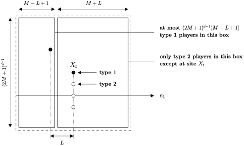
Figure 5: Picture related to the proof of Lemma 12.

Case 1. Assume that $L_{t}=L\in[1,M]$. Then the number of type 1 neighbors of the tagged player is bounded by the number of vertices in the leftmost rectangle in the picture,

$$f_{1}(X_{t},\xi_{t})\leq N^{-1}(2M+1)^{d-1}(M-L+1).$$

Therefore the rate at which the strategy at $X_{t}$ changes from $1\to 2$ is

$$c(X_{t},\xi_{t}) \leq N^{-2}(-a_{11})\max\bigl{\{}z(N-z)\dvtx z\leq(2M+1)^{d-1}(M-L+1)\bigr{\}}$$

$$= N^{-2}(-a_{11})(2M+1)^{d-1}(M-L+1)\bigl{(}(2M+1)^{d-1}(M+L)-1\bigr{)}.$$

Since such a transition causes the tagged player to jump $L$ units to the left or equivalently the first coordinate $\pi_{1}(X_{t})$ of the process $X_{t}$ to decrease by the amount $L$, the previous inequality also gives the following bound almost surely on the transition rate:

$$\lim_{h\to 0}h^{-1}P\bigl{(}\pi_{1}(X_{t+h})-\pi_{1}(X_{t})=-L|\xi_{t}\mbox{ and }L_{t}=L\in[1,M]\bigr{)}$$

$$\qquad\leq N^{-2}(-a_{11})(2M+1)^{d-1}(M-L+1)\bigl{(}(2M+1)^{d-1}(M+L)-1\bigr{)}.$$

In addition, each site $x$ occupied by a player of type 2 in the neighborhood of $X_{t}$ has at least one neighbor of type 1, namely the tagged player, therefore the rate at which the strategy at such a neighbor $x$ changes from $2\to 1$ is at least equal to

$$c(x,\xi_{t}) \geq N^{-2}(-a_{22})\min\bigl{\{}z(N-z)\dvtx z\neq 0\bigr{\}}$$

$$= N^{-2}(-a_{22})(N-1)=N^{-2}(-a_{22})\bigl{(}(2M+1)^{d}-2\bigr{)}.$$

Since such a transition causes the tagged player to jump to $x$ when $\pi_{1}(x)>\pi_{1}(X_{t})$ and since the number of such neighbors of the tagged player is given by

$$\operatorname{card}\bigl{\{}x\in N_{X_{t}}\dvtx\pi_{1}(x)=\pi_{1}(X_{t})+j\mbox{ and }x\notin\xi_{t}\bigr{\}}=(2M+1)^{d-1}$$

for all $j=1,2,\ldots,M$, we deduce that

$$\lim_{h\to 0}h^{-1}P\bigl{(}\pi_{1}(X_{t+h})-\pi_{1}(X_{t})=j|\xi_{t}\bigr{)}$$

(38)

$$\qquad\geq N^{-2}(-a_{22})\bigl{(}(2M+1)^{d}-2\bigr{)}(2M+1)^{d-1}$$

almost surely for all $j=1,2,\ldots,M$. Using as previously mentioned that (4) is the only transition that can decrease the first coordinate of the tagged player and summing the transition rates in (4) over all the possible values of $j$, we deduce that, almost surely,

$$\lim_{h\to 0}h^{-1}E\bigl{(}\pi_{1}(X_{t+h})-\pi_{1}(X_{t})|\xi_{t}\mbox{ and }L_{t}=L\in[1,M]\bigr{)}$$

$$\qquad\geq(-L)\lim_{h\to 0}h^{-1}P\bigl{(}\pi_{1}(X_{t+h})-\pi_{1}(X_{t})=-L|\xi_{t}\mbox{ and }L_{t}=L\in[1,M]\bigr{)}$$

$$\qquad\quad{}+\sum_{j=1}^{M}j\lim_{h\to 0}h^{-1}P\bigl{(}\pi_{1}(X_{t+h})-\pi_{1}(X_{t})=j|\xi_{t}\bigr{)}$$

$$\qquad\geq(-L)N^{-2}(-a_{11})(2M+1)^{d-1}(M-L+1)\bigl{(}(2M+1)^{d-1}(M+L)-1\bigr{)}$$

$$\qquad\quad{}+\sum_{j=1}^{M}jN^{-2}(-a_{22})\bigl{(}(2M+1)^{d}-2\bigr{)}(2M+1)^{d-1}.$$

Expanding and simplifying the right-hand side gives

$$\lim_{h\to 0}h^{-1}E\bigl{(}\pi_{1}(X_{t+h})-\pi_{1}(X_{t})|\xi_{t}\mbox{ and }L_{t}=L\in[1,M]\bigr{)}$$

$$\qquad\geq N^{-2}(2M+1)^{d-1}\bigl{[}a_{11}L(M-L+1)\bigl{(}(2M+1)^{d-1}(M+L)-1\bigr{)}$$

$$\hskip 124.0pt\qquad{}-a_{22}(1/2)M(M+1)\bigl{(}(2M+1)^{d}-2\bigr{)}\bigr{]}.$$

Using that $L(M-L+1)\leq(1/4)(M+1)^{2}$ and $M+L\leq 2M$, we obtain

$$\lim_{h\to 0}h^{-1}E\bigl{(}\pi_{1}(X_{t+h})-\pi_{1}(X_{t})|\xi_{t}\mbox{ and }L_{t}=L\in[1,M]\bigr{)}$$

$$\qquad\geq N^{-2}(2M+1)^{d-1}\bigl{[}a_{11}(1/4)(M+1)^{2}\bigl{(}2M(2M+1)^{d-1}-1\bigr{)}$$

$$\hskip 124.0pt{}-a_{22}(1/2)M(M+1)\bigl{(}(2M+1)^{d}-2\bigr{)}\bigr{]}$$

$$\qquad=N^{-2}(2M+1)^{d-1}(1/4)(M+1)$$

$$\qquad\quad{}\times\bigl{(}a_{11}(M+1)\bigl{(}2M(2M+1)^{d-1}-1\bigr{)}-a_{22}(2M)\bigl{(}(2M+1)^{d}-2\bigr{)}\bigr{)}$$

$$\qquad=N^{-2}(2M+1)^{d-1}(1/4)(M+1)^{2}\bigl{(}2M(2M+1)^{d-1}-1\bigr{)}$$

$$\qquad\quad{}\times\bigl{(}a_{11}-c(M,d)a_{22}\bigr{)}>0$$

almost surely whenever (35) holds.

Case 2. Assume that $L_{t}=L\notin[1,M]$. Then we have the following alternative:

• $L=0$, and then there are at least two vertices in the set $R_{t}$.

• $L>M$, and then the tagged player has only type 2 players in her neighborhood and therefore changes her strategy at rate zero.

In either case, $\pi_{1}(X_{t})$ cannot decrease, so (4) implies that

$$\lim_{h\to 0}h^{-1}E\bigl{(}\pi_{1}(X_{t+h})-\pi_{1}(X_{t})|\xi_{t}\mbox{ and }L_{t}=L\notin[1,M]\bigr{)}$$

$$\qquad\geq\sum_{j=1}^{M}j\lim_{h\to 0}h^{-1}P\bigl{(}\pi_{1}(X_{t+h})-\pi_{1}(X_{t})=j|\xi_{t}\bigr{)}$$

$$\qquad\geq N^{-2}(2M+1)^{d-1}(1/4)(M+1)(-a_{22})(2M)\bigl{(}(2M+1)^{d}-2\bigr{)}>0$$

almost surely whenever (35) holds. This completes the proof.

The previous lemma is similar to pages 1247–1248 in neuhauser_pacala_1999 . There, the authors conclude that we can bring a particle—the tagged player in our case—close to the target $Ke_{1}$. This is obvious in one dimension. In higher dimensions, the idea is to use the lemma to increase the first coordinate of the tagged player up to $K$ and then apply the lemma again along each of the other $d-1$ axes to bring the tagged player close to the target. However, since we do not have control on the position of the tagged player in the direction orthogonal to $e_{1}$ while moving along the first axis, the conclusion is not obvious. To prove that we can bring a type 1 player close to the target in higher dimensions, we look instead at the Euclidean distance between the target and the type 1 player the closest to the target. We now call $X_{t}$ the position of one of the type 1 players chosen uniformly at random among the ones who are the closest to $Ke_{1}$, called again the tagged player, and prove that

$$\qquad\lim_{h\to 0}\sup_{x\notin B_{2}(Ke_{1},K/5)}h^{-1}E(D_{t+h}-D_{t}|X_{t}=x)\leq-\mu\qquad\mbox{for some $\mu>0$},$$ (39)

where $D_{t}:=\operatorname{dist}(X_{t},Ke_{1})=$ Euclidean distance between $X_{t}$ and $Ke_{1}$ and where $\Omega_{K}$ is a set of configurations in which the tagged player is far from the target,

$$\Omega_{K}:=\bigl{\{}\eta\subset\mathbb{Z}^{d}\dvtx\eta\cap B_{2}(Ke_{1},K/5)=\varnothing\bigr{\}}\qquad\mbox{for $K$ large}.$$

Although our proof relies on basic trigonometry, the algebra is somewhat messy, so we only prove the result in the two-dimensional nearest neighbor case. Hopefully, the next lemma will convince the reader that, even if the players are located on a square lattice, the type 1 players spread not only along each axis but also along any arbitrary direction provided condition (35) holds.

Lemma 13.

Assume that $(M,d)=(1,2)$, and (35) holds. Then, (39) holds for all $K$ large.

The proof is based on the construction given in Figure 6. Let:

$$C := \mbox{the circle with center $Ke_{1}$ going through $X_{t}$},$$

$$\Delta := \mbox{the tangent line to the circle $C$ going through $X_{t}$},$$

$$\Gamma := \mbox{the straight line parallel to the tangent $\Delta$ going through $Ke_{1}$}.$$

The first ingredient is to observe that, on the event that $\xi_{t}\in\Omega_{K}$,

$$\lim_{h\to 0}\sup_{x\notin B_{2}(Ke_{1},K/5)}h^{-1}E(D_{t+h}-D_{t}|X_{t}=x)$$

(40)

$$\qquad\approx\lim_{h\to 0}\sup_{x\notin B_{2}(Ke_{1},K/5)}h^{-1}E\bigl{(}\operatorname{dist}(X_{t+h},\Gamma)-\operatorname{dist}(X_{t},\Gamma)|X_{t}=x\bigr{)}$$

when the parameter $K$ is large, so it suffices to prove the result for the right-hand side. To estimate the drift, note that the straight line $\Delta$ divides the neighborhood of $X_{t}$ into two sets of four vertices: as indicated on the left-hand side of the figure, we denote by $y_{i}$ the four vertices the closest to the target $Ke_{1}$ and we denote by $x_{i}$ the other four vertices in such a way that

$$l_{i}:=\operatorname{dist}(y_{i},\Delta)=\operatorname{dist}(x_{i},\Delta)\qquad\mbox{for }i=1,2,3,4.$$

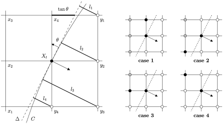
Figure 6: Picture related to the proof of Lemma 13.

Defining the angle $\theta$ as in the picture, some basic trigonometry shows that

$$l_{1} = (1-\tan\theta)\cos\theta,\qquad l_{2}=\cos\theta,$$

$$l_{3} = (1+\tan\theta)\cos\theta,\qquad l_{4}=\tan\theta\cos\theta.$$

We may assume that $0\leq\theta\leq\pi/4$ and so $\tan\theta\in[0,1]$ since any other configuration can be deduced from a rotation of this configuration. Note that all four players at sites $y_{i}$ must follow strategy 2, which gives $2^{4}=16$ possible configurations in the neighborhood of $X_{t}$. To find a bound for the drift, we only distinguish four types of configurations (see Figure 6).

• Case 1. Assume that $x_{4}\in\xi_{t}$. Then

  $$\lim_{h\to 0}\sup_{x\notin B_{2}(Ke_{1},K/5)}h^{-1}E\bigl{(}\operatorname{dist}(X_{t+h},\Gamma)-\operatorname{dist}(X_{t},\Gamma)|X_{t}=x\bigr{)}$$

  $$\qquad\leq(-a_{11})(16/64)l_{4}-(-a_{22})$$

  $$\quad\qquad{}\times\bigl{(}(12/64)l_{1}+(12/64)l_{2}+(7/64)l_{3}+(7/64)l_{4}\bigr{)}.$$

  Using (4), we deduce that

  $$\lim_{h\to 0}\sup_{x\notin B_{2}(Ke_{1},K/5)}h^{-1}E\bigl{(}\operatorname{dist}(X_{t+h},\Gamma)-\operatorname{dist}(X_{t},\Gamma)|X_{t}=x\bigr{)}$$

  $$\qquad\leq(1/64)\cos\theta\bigl{(}-a_{11}(16\tan\theta)+a_{22}(31+2\tan\theta)\bigr{)}<0$$

  whenever $a_{11}>(33/16)a_{22}$ which holds if $a_{11}>c(1,2)a_{22}=(7/5)a_{22}$.

• Case 2. Assume that $x_{4}\notin\xi_{t}$ and $x_{1}\in\xi_{t}$. Then

  $$\lim_{h\to 0}\sup_{x\notin B_{2}(Ke_{1},K/5)}h^{-1}E\bigl{(}\operatorname{dist}(X_{t+h},\Gamma)-\operatorname{dist}(X_{t},\Gamma)|X_{t}=x\bigr{)}$$

  $$\qquad\leq(1/64)\cos\theta\bigl{(}-a_{11}\times 15l_{1}+a_{22}\times(7l_{1}+7l_{2}+7l_{3}+12l_{4})\bigr{)}$$

  $$\qquad=(1/64)\cos\theta\bigl{(}-a_{11}(15-15\tan\theta)+a_{22}(21+12\tan\theta)\bigr{)}<0$$

  whenever $a_{11}>c(1,2)a_{22}=(7/5)a_{22}$.

• Case 3. Assume that $x_{4},x_{1}\notin\xi_{t}$ and $x_{2}\in\xi_{t}$. Then

  $$\lim_{h\to 0}\sup_{x\notin B_{2}(Ke_{1},K/5)}h^{-1}E\bigl{(}\operatorname{dist}(X_{t+h},\Gamma)-\operatorname{dist}(X_{t},\Gamma)|X_{t}=x\bigr{)}$$

  $$\qquad\leq(1/64)\cos\theta\bigl{(}-a_{11}\times 12l_{2}+a_{22}\times(7l_{1}+7l_{2}+7l_{3}+12l_{4})\bigr{)}$$

  $$\qquad=(1/64)\cos\theta\bigl{(}-12a_{11}+a_{22}(21+12\tan\theta)\bigr{)}<0$$

  whenever $a_{11}>(7/4)a_{22}$ which holds if $a_{11}>c(1,2)a_{22}=(7/5)a_{22}$.

• Case 4. Assume that $x_{4},x_{1},x_{2}\notin\xi_{t}$ and $x_{3}\in\xi_{t}$. Then

  $$\lim_{h\to 0}\sup_{x\notin B_{2}(Ke_{1},K/5)}h^{-1}E\bigl{(}\operatorname{dist}(X_{t+h},\Gamma)-\operatorname{dist}(X_{t},\Gamma)|X_{t}=x\bigr{)}$$

  $$\qquad\leq(1/64)\cos\theta\bigl{(}-a_{11}\times 7l_{2}+a_{22}\times(7l_{1}+7l_{2}+7l_{3}+7l_{4})\bigr{)}$$

  $$\qquad=(1/64)\cos\theta\bigl{(}-a_{11}(7+7\tan\theta)+a_{22}(21+7\tan\theta)\bigr{)}<0$$

  whenever $a_{11}>2a_{22}$ which holds if $a_{11}>c(1,2)a_{22}=(7/5)a_{22}$.

This, together with the approximation (4), implies the lemma.

We now use Lemmas 12 and 13 to prove that, with probability close to one when $K$ is large, the tagged player is located in a certain Euclidean ball with center $Ke_{1}$ at a deterministic time proportional to $K$. This is done in Lemmas 14–16 below where we successively prove that the tagged player hits a subset of the target region in a short time, does not leave a certain larger ball centered at zero, and stays in the target region for a long time. The second step is needed to ensure that the events under consideration are measurable with respect to the graphical representation in a finite space–time box, which is a key to obtaining a coupling between the process and oriented percolation with a finite range of dependence. For every positive integer $K$, define

$$\tau_{K}:=\inf\bigl{\{}t\dvtx X_{t}\in B_{2}(Ke_{1},2K/5)\bigr{\}}=\inf\{t\dvtx D_{t}<2K/5\}.$$

Lemma 14.

Assume (35). There exist $c,C_{1}<\infty$ and $\gamma_{1}>0$ such that

$$P\bigl{(}\tau_{K}\geq cK|X_{0}\in B_{2}(0,3K/5)\bigr{)}\leq C_{1}\exp(-\gamma_{1}K)\qquad\mbox{for all $K$ large}.$$

According to Lemmas 12 and 13,

$$\qquad\lim_{h\to 0}\sup_{x\notin B_{2}(Ke_{1},K/5)}h^{-1}E(D_{t+h}-D_{t}|X_{t}=x)\leq-\mu\qquad\mbox{for some }\mu>0$$ (42)

from which it follows that

$$ED_{t}\leq D_{0}-\mu t\qquad\mbox{for all }t<\mu^{-1}(D_{0}-K/5).$$

Using in addition that the number of jumps of the process $(D_{t})$ dominates stochastically the number of jumps of a Poisson process with positive intensity, large deviation estimates for the Poisson distribution imply that

$$P\bigl{(}\tau_{K}\geq 2\mu^{-1}K|X_{0}\in B_{2}(0,3K/5)\bigr{)}$$

$$\qquad\leq P\bigl{(}D_{t}\geq K/5\mbox{ for all }t<2\mu^{-1}K|D_{0}\leq 7K/5\bigr{)}\leq C_{1}\exp(-\gamma_{1}K)$$

for suitable constants $C_{1}<\infty$ and $\gamma_{1}>0$ and all $K$ sufficiently large.

Lemma 15.

Assume (35). There exist $C_{2}<\infty$ and $\gamma_{2}>0$ such that

$$P\bigl{(}D_{t}\geq 2K\mbox{ for some }t\in(0,cK)|X_{0}\in B_{2}(0,3K/5)\bigr{)}\leq C_{2}\exp(-\gamma_{2}K)$$

for all $K$ sufficiently large, and where $c$ is as in Lemma 14.

First, we introduce the stopping times

$$\sigma_{K}:=\inf\{t\dvtx D_{t}\geq 2K\}\quad\mbox{and}\quad T_{K}:=\inf(\tau_{K},\sigma_{K})$$

and the process stopped at time $T_{K}$

$$Z_{t}:=\exp(aD_{t})\mathbf{1}\{t<T_{K}\}+\exp(aD_{T_{K}})\mathbf{1}\{t\geq T_{K}\}.$$

As in Lemma 6, the key to the proof is to find a constant $a>0$ such that the process $(Z_{t})$ is a supermartingale with respect to the natural filtration of the process $(\xi_{t})$ and then apply the optimal stopping theorem. To prove the existence of such a constant, we introduce

$$\Phi(a):=\lim_{h\to 0}h^{-1}E\bigl{(}Z_{t+h}(a)-Z_{t}(a)|\xi_{t}\bigr{)}$$

and observe that, for all $t<T_{K}$,

$$\Phi(a) = \sum_{x\in\mathbb{Z}^{d}}\bigl{(}\exp\bigl{(}a\operatorname{dist}(X_{t}+x,Ke_{1})\bigr{)}-\exp\bigl{(}a\operatorname{dist}(X_{t},Ke_{1})\bigr{)}\bigr{)}$$

$$\hskip 18.0pt{}\times\lim_{h\to 0}h^{-1}P(X_{t+h}-X_{t}=x|\xi_{t}).$$

Recalling (42) and using that $D_{t}\geq K/5$ for all $t<T_{K}$, we deduce that

$$\Phi^{\prime}(0) = \sum_{x\in\mathbb{Z}^{d}}\bigl{(}\operatorname{dist}(X_{t}+x,Ke_{1})-\operatorname{dist}(X_{t},Ke_{1})\bigr{)}\lim_{h\to 0}h^{-1}P(X_{t+h}-X_{t}=x|\xi_{t})$$

$$= \lim_{h\to 0}h^{-1}E(D_{t+h}-D_{t}|\xi_{t})\leq-\mu<0\qquad\mbox{almost surely}.$$

Since in addition $\Phi(0)=0$, there exists $a_{0}>0$ fixed from now on such that

$$\Phi(a_{0}):=\lim_{h\to 0}h^{-1}E(Z_{t+h}-Z_{t}|\xi_{t})\leq 0\qquad\mbox{almost surely},$$

which implies that $(Z_{t})$ is a supermartingale for this value of $a$. Since the stopping time $T_{K}$ is almost surely finite, the optimal stopping theorem further implies that

$$EZ_{T_{K}} \leq EZ_{0}=E\exp(a_{0}X_{0})\leq\exp\bigl{(}a_{0}(K+3K/5)\bigr{)}=\exp\bigl{(}a_{0}(8K/5)\bigr{)},$$

$$EZ_{T_{K}} \geq \exp(2a_{0}K)P(\sigma_{K}<\tau_{K})+\exp\bigl{(}a_{0}(2K/5-M)\bigr{)}P(\tau_{K}<\sigma_{K})$$

$$\geq \exp(2a_{0}K)P(\sigma_{K}<\tau_{K})+\exp\bigl{(}a_{0}(2K/5-M)\bigr{)}\bigl{(}1-P(\sigma_{K}<\tau_{K})\bigr{)}$$

from which we deduce that

$$P(\sigma_{K}<\tau_{K}) \leq \bigl{[}\exp\bigl{(}a_{0}(8K/5)\bigr{)}-\exp\bigl{(}a_{0}(2K/5-M)\bigr{)}\bigr{]}$$

$${}\times\bigl{[}\exp(2a_{0}K)-\exp\bigl{(}2a_{0}(2K/5-M)\bigr{)}\bigr{]}^{-1}$$

$$= \bigl{[}\exp\bigl{(}a_{0}(6K/5+M)-1\bigr{)}\bigr{]}\bigl{[}\exp\bigl{(}a_{0}(8K/5+M)-1\bigr{)}\bigr{]}^{-1}$$

$$\leq \exp(-2a_{0}K/5).$$

Since the probability that the number of jumps of the tagged player by time $cK$ exceeds a certain multiple of $K$ also has exponential decay, the result follows.

Lemma 16.

Assume (35). There exist $C_{3}<\infty$ and $\gamma_{3}>0$ such that

$$P\bigl{(}D_{t}\geq 3K/5\mbox{ for some }t\in(\tau_{K},cK)|\tau_{K}<cK\bigr{)}\leq C_{3}\exp(-\gamma_{3}K)$$

for all $K$ sufficiently large.

The result directly follows by observing that

$$P\bigl{(}D_{t}\geq 3K/5\mbox{ for some }t\in(\tau_{K},cK)|\tau_{K}<cK\bigr{)}$$

$$\qquad\leq P\bigl{(}D_{t}\geq 3K/5\mbox{ for some }t\in(0,cK)|D_{0}<2K/5\bigr{)}$$

and by following the argument of the proof of Lemma 15 but using

$$\tau^{\prime}_{K}:=\inf\{t\dvtx D_{t}<K/5\}\quad\mbox{and}\quad\sigma^{\prime}_{K}:=\inf\{t\dvtx D_{t}\geq 3K/5\}$$

in place of the stopping times $\tau_{K}$ and $\sigma_{K}$.

With Lemmas 14–16, we are now ready to couple the process properly rescaled in space and time with oriented site percolation. Denote by $\mathbb{W}_{n}^{1-\varepsilon}$ the set of wet sites at level $n$ in a one dependent oriented site percolation process on $\mathcal{H}_{1}$ in which sites are open with probability $1-\varepsilon$. Recall that a site is said to be wet if it can be reached from level zero by a path of open sites.

Lemma 17.

Assume (35), and let $\varepsilon>0$. Then, for all $K$ sufficiently large, the process can be coupled with oriented site percolation in such a way that

$$\mathbb{W}_{n}^{1-\varepsilon}\subset\mathbb{X}_{n}\qquad\mbox{for all }n\geq 0\mbox{ whenever }\mathbb{X}_{0}=\mathbb{W}_{0}^{1-\varepsilon}.$$

Let $\Omega(z,n)$ denote the event that site $(z,n)\in H$ is occupied, that is,

$$\xi_{cnK}\cap B_{2}(Kz,3K/5)\neq\varnothing.$$

Lemmas 14 and 16 imply the existence of a collection of events $G(z,n)$ measurable with respect to the graphical representation of the process such that: [(1)]

for all $K$ sufficiently large, $P(G(z,n))\geq 1-\varepsilon$, and such that

we have the inclusions of events

$$G(z,n)\cap\Omega(z,n)\subset\Omega(z\pm e_{i},n+1)\qquad\mbox{for all }i=1,2,\ldots,d.$$

In addition, Lemma 15 implies that these events can be chosen so that [(1)]

$G(z,n)$ is measurable with respect to the graphical representation in

$$B_{2}(Kz,2K)\times\bigl{[}cnK,c(n+1)K\bigr{]}=(Kz,cnK)+B_{2}(0,2K)\times[0,cK].$$

These are the assumptions of Theorem 4.3 in Durrett durrett_1995 , from which the existence of the coupling between the two processes directly follows.

In the next lemma, which recalls the statement of Theorem 5, we return to the process with general payoffs. The proof relies on the previous lemma, the symmetry of the evolution rules of the spatial game and a perturbation argument.

Lemma 18.

For all $a_{12}$ and $a_{21}$ there exists $m>0$ such that coexistence occurs when

$$c(M,d)a_{22}<a_{11}<-m\quad\mbox{and}\quad c(M,d)a_{11}<a_{22}<-m.$$

First, we fix $\varepsilon<(1/2)(1-p_{c})$ positive where $p_{c}<1$ is the critical value of the oriented site percolation process introduced above. To prove that both strategies can survive simultaneously, we extend our previous definition of occupied site by calling $(z,n)\in H$ a good site whenever

$$x\in\eta_{cnK}\quad\mbox{and}\quad y\notin\eta_{cnK}\qquad\mbox{for some }x,y\in B_{2}(Kz,3K/5).$$

Denote by $\mathbb{Y}_{n}$ the set of good sites at level $n$. The symmetry of the evolution rules implies that the conclusion of Lemma 17 holds for $\mathbb{Y}_{n}$ provided that

$$a_{12} = a_{21}=0\quad\mbox{and}\quad c(M,d)a_{22}<a_{11}<-1\quad\mbox{and}$$

$$c(M,d)a_{11} < a_{22}<-1.$$

Even though (weak) survival of both strategies when $a_{12}=a_{21}=0$ is in fact trivial since in this case a player isolated from players of her own type cannot change her strategy, we point out that the coupling with oriented site percolation is needed to obtain the full coexistence region. Indeed, the parameter $K$ being fixed such that the process dominates one dependent oriented site percolation with parameter $1-\varepsilon$, the continuity of the transition rates with respect to the payoffs implies the existence of a small $\rho=\rho(K)>0$ and a coupling of the processes such that

$$\mathbb{W}_{n}^{1-2\varepsilon}\subset\mathbb{Y}_{n}\qquad\mbox{for all }n\geq 0\mbox{ whenever }\mathbb{Y}_{0}=\mathbb{W}_{0}^{1-2\varepsilon}$$ (44)

in a perturbation of the parameter region (4) given by

$$-\rho < a_{12},a_{21}<\rho\quad\mbox{and}\quad c(M,d)a_{22}<a_{11}<-1\quad\mbox{and}$$

$$c(M,d)a_{11} < a_{22}<-1.$$

In particular, letting $f\dvtx 2^{H}=\mbox{power set of }H\to\{0,1\}$ be defined by

$$f\bigl{(}\{\mathbb{W}_{n}\dvtx n\geq 0\}\bigr{)}:=\mathbf{1}\bigl{\{}\operatorname{card}(n\dvtx z\in\mathbb{W}_{n})=\infty\mbox{ for all }z\in\mathbb{Z}^{d}\bigr{\}}$$ (46)

and using (44) and the monotonicity of $f$, we obtain that for all $(x,t)\in\mathbb{Z}^{d}\times\mathbb{R}_{+}$,

$$P(x\in\eta_{s_{1}}\mbox{ and }x\notin\eta_{s_{2}}\mbox{ for some }s_{1},s_{2}>t)$$

$$\qquad\geq P\bigl{(}\operatorname{card}(n\dvtx z\in\mathbb{Y}_{n})=\infty\mbox{ for all }z\in\mathbb{Z}^{d}\bigr{)}=Ef\bigl{(}\{\mathbb{Y}_{n}\dvtx n\geq 0\}\bigr{)}$$

$$\qquad\geq Ef\bigl{(}\bigl{\{}\mathbb{W}_{n}^{1-2\varepsilon}\dvtx n\geq 0\bigr{\}}\bigr{)}=P\bigl{(}\operatorname{card}\bigl{(}n\dvtx z\in\mathbb{W}_{n}^{1-2\varepsilon}\bigr{)}=\infty\mbox{ for all }z\in\mathbb{Z}^{d}\bigr{)}=1$$

since infinitely many sites are wet at level zero and $1-2\varepsilon>p_{c}$. Note also that the first inequality follows from the fact that if a site is good, then the corresponding space–time region obtained through rescaling contains both strategies, so the probability that any given vertex $x$ in this region changes its strategy after one time unit is bounded from below by a positive constant. This proves coexistence of both strategies in the parameter region (4). To deal with the general case when both payoffs $a_{12}$ and $a_{21}$ are arbitrary, we fix a sufficiently large $m>0$ such that

$$a_{12}\in(-m\rho,m\rho)\quad\mbox{and}\quad a_{21}\in(-m\rho,m\rho).$$

Since the long-term behavior remains unchanged by speeding up time by $m$, that is, multiplying all the payoffs by the same factor $m$, we obtain coexistence in the parameter region

$$c(M,d)a_{22}<a_{11}<-m\quad\mbox{and}\quad c(M,d)a_{11}<a_{22}<-m.$$

This proves the lemma and Theorem 5.

5 Proof of Theorem 2

This section is devoted to the proof of Theorem 2. We first prove that, under the assumption of the theorem, strategy 1 survives. The key to obtaining this partial result is to observe that, when the first payoff $a_{11}=1$ while the other payoffs are equal to zero, the spatial game starting from suitable initial configurations dominates stochastically a Richardson model richardson_1973 . To also prove extinction of strategy 2, we use an idea of Lanchier lanchier_2012 that extends from discrete-time to continuous-time processes a result of Durrett durrett_1992 which states that sites which are not wet do not percolate for oriented site percolation models in which sites are open with probability close to one. Throughout this section, to shorten a little bit the expression of certain events, we let

$$B_{r}:=[-r,r]^{d}\qquad\mbox{for all }r>0.$$

The spatial boxes involved in the block construction in both this section and the next section are translations of these boxes for an appropriate radius $r$.

Lemma 19.

Let $\varepsilon>0$ and $a_{11}=1$. Then there exist $K,c,\rho>0$ such that

$$P\bigl{(}\eta_{t}\not\supset B_{2K}\mbox{ for some }t\in(cK,2cK)|\eta_{0}\supset B_{K}\bigr{)}\leq\varepsilon\qquad\mbox{for all }\bar{a}_{11}\in(-\rho,\rho)^{3}.$$

We introduce the following auxiliary processes:

• the spatial game $\xi_{t}$ with payoffs $a_{11}=1$ and $\bar{a}_{11}=0$ and

• the Richardson model $\zeta_{t}$ with flip rate

  $$c_{\mathrm{RM}}(x,\zeta)=\beta^{2}f_{1}(x,\zeta)\mathbf{1}\{x\notin\zeta\}\qquad\mbox{where }\beta:=\bigl{(}(2M+1)^{d}-1\bigr{)}^{-1}.$$

In the process $\xi_{t}$ all type 2 players have a zero payoff while each type 1 player with at least one type 1 neighbor has a payoff equal to $\beta$ from which it follows that

$$c_{\mathrm{SG}}(x,\xi) = 0\qquad\mbox{if }x\in\xi,$$

$$c_{\mathrm{SG}}(x,\xi) \geq \beta^{2}\qquad\mbox{if }x\notin\xi\mbox{ and }f_{1}(y,\xi)\neq 0\mbox{ for some }y\in\xi\cap N_{x}.$$

Since in addition the property that each type 1 player has at least one type 1 neighbor is preserved by the dynamics of the processes, we deduce the existence of a coupling $(\zeta,\xi)$ such that

$$P(\zeta_{t}\subset\xi_{t}|\zeta_{0}=\xi_{0}=B_{K})=1.$$ (47)

In other respects, the shape theorem richardson_1973 for the Richardson model implies the existence of a positive constant $c>0$ fixed from now on such that

$$P\bigl{(}\zeta_{t}\not\supset B_{2K}\mbox{ for some }t\in(cK,2cK)|\zeta_{0}\supset B_{K}\bigr{)}$$

$$\qquad=P(\zeta_{cK}\not\supset B_{2K}|\zeta_{0}\supset B_{K})$$

$$\qquad\leq P\bigl{(}\zeta_{cK}\not\supset B_{2K}|\zeta_{0}=\{0\}\bigr{)}\leq\varepsilon/2\qquad\mbox{for all $K$ large},$$

where the equality between the first two lines holds because infected sites in the Richardson model do not recover. In view of (47), the same holds for the spatial game, that is,

$$P\bigl{(}\xi_{t}\not\supset B_{2K}\mbox{ for some }t\in(cK,2cK)|\xi_{0}\supset B_{K}\bigr{)}\leq\varepsilon/2$$ (48)

for all $K$ large. Now, we fix $K$ such that (48) holds. The scale parameter $K$ and the constant $c$ being fixed, the continuity of the transition rates of the spatial game with respect to the payoffs implies the existence of a small constant $\rho>0$ and a coupling $(\eta,\xi)$ such that

$$P(\eta_{t}\cap B_{2K}\neq\xi_{t}\cap B_{2K}\mbox{ for some }t\leq 2cK|\eta_{0}=\xi_{0})\leq\varepsilon/2$$ (49)

whenever $\bar{a}_{11}\in(-\rho,\rho)^{3}$. Combining (48) and (49) gives

$$P\bigl{(}\eta_{t}\not\supset B_{2K}\mbox{ for some }t\in(cK,2cK)|\eta_{0}\supset B_{K}\bigr{)}$$

$$\qquad\leq P\bigl{(}\xi_{t}\not\supset B_{2K}\mbox{ for some }t\in(cK,2cK)|\xi_{0}\supset B_{K}\bigr{)}$$

$$\qquad\quad{}+P(\eta_{t}\cap B_{2K}\neq\xi_{t}\cap B_{2K}\mbox{ for some }t\leq 2cK|\eta_{0}=\xi_{0})$$

$$\qquad\leq\varepsilon$$

for all $a_{11}\in(-\rho,\rho)^{3}$. This completes the proof.

To deduce survival of strategy 1 from Lemma 19 and under the assumptions of the lemma, we now declare a site $(z,n)\in H$ to be occupied whenever

$$x\in\eta_{t}\qquad\mbox{for all }(x,t)\in(Kz,cnK)+B_{K}\times(0,cK)$$

and define the set $\mathbb{X}_{n}$ of occupied sites at level $n$ as in (36). Repeating the proof of Lemma 17 but using Lemma 19 in place of Lemmas 14–16 directly gives the following result.

Lemma 20.

Let $\varepsilon>0$ and $a_{11}=1$. Then there exist $K,c,\rho>0$ and a coupling of the spatial game with one dependent oriented site percolation such that

$$\mathbb{W}_{n}^{1-\varepsilon}\subset\mathbb{X}_{n}\qquad\mbox{for all }n\mbox{ whenever }\mathbb{X}_{0}=\mathbb{W}_{0}^{1-\varepsilon}\mbox{ and }\bar{a}_{11}\in(-\rho,\rho)^{3}.$$

Taking $\varepsilon>0$ strictly smaller than one minus the critical value of one dependent oriented site percolation, and using the coupling given in the previous lemma for this value of $\varepsilon$ as well as the monotone function $f$ defined in (46), we obtain that, for all $(x,t)\in\mathbb{Z}^{d}\times\mathbb{R}_{+}$

$$P(x\in\eta_{s}\mbox{ for some }s>t)$$

$$\qquad\geq P\bigl{(}\operatorname{card}(n\dvtx z\in\mathbb{X}_{n})=\infty\mbox{ for all }z\in\mathbb{Z}^{d}\bigr{)}=Ef\bigl{(}\{\mathbb{X}_{n}\dvtx n\geq 0\}\bigr{)}$$

$$\qquad\geq Ef\bigl{(}\bigl{\{}\mathbb{W}_{n}^{1-\varepsilon}\dvtx n\geq 0\bigr{\}}\bigr{)}=P\bigl{(}\operatorname{card}\bigl{(}n\dvtx z\in\mathbb{W}_{n}^{1-\varepsilon}\bigr{)}=\infty\mbox{ for all }z\in\mathbb{Z}^{d}\bigr{)}=1.$$

This proves that strategy 1 survives but not that it wins since there is a positive density of closed sites, which does not exclude the possibility of having a positive density of sites which are not occupied, and so the presence of type 2 players, at arbitrarily large times. To prove extinction of the type 2 players, we use the coupling above together with an idea of Lanchier lanchier_2012 that extends a result of Durrett durrett_1992 . This is done in the next lemma.

Lemma 21.

Let $a_{11}=1$. Then, there exists $\rho>0$ small such that

$$\lim_{t\to\infty}P(x\notin\eta_{t})=0\qquad\mbox{for all }x\in\mathbb{Z}^{d}\mbox{ whenever }\bar{a}_{11}\in(-\rho,\rho)^{3}.$$

Following an idea of Lanchier lanchier_2012 we introduce the new oriented graph $\mathcal{H}_{2}$ with the same vertex set as the oriented graph $\mathcal{H}_{1}$ but in which there is an oriented edge

$$(z,n)\to\bigl{(}z^{\prime},n^{\prime}\bigr{)}$$

$$\eqntext{\mbox{if and only if }\bigl{(}z^{\prime}=z\pm e_{i}\mbox{ for some }i=1,2,\ldots,d\mbox{ and }n^{\prime}=n+1\bigr{)}}$$ (50)

$$\eqntext{\mbox{or }\bigl{(}z^{\prime}=z\pm 2e_{i}\mbox{ for some }i=1,2,\ldots,d\mbox{ and }n^{\prime}=n\bigr{)}.}$$ (51)

See the right-hand side of Figure 7 for a picture in $d=1$.

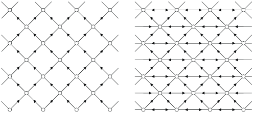
Figure 7: Picture of the graphs $\mathcal{H}_{1}$ and $\mathcal{H}_{2}$ in dimension $d=1$.

We say that a site is dry if it is not wet for oriented site percolation on the graph $\mathcal{H}_{1}$. Also, we write

$$(w,0)\to_{j}(z,n)\qquad\mbox{for }j=1,2,$$

and say that there is a dry path in $\mathcal{H}_{j}$ connecting both sites if there exist

$$(z_{0},0)=(w,0),(z_{1},n_{1}),\ldots,(z_{k-1},n_{k-1}),(z_{k},n_{k})=(z,n)\in H$$

such that the following two conditions hold: [(1)]

$(z_{i},n_{i})\to(z_{i+1},n_{i+1})$ is an oriented edge in $\mathcal{H}_{j}$ for all $i=0,1,\ldots,k-1$, and

the site $(z_{i},n_{i})$ is dry for all $i=0,1,\ldots,k$. Note that a dry path in $\mathcal{H}_{1}$ is also a dry path in $\mathcal{H}_{2}$, but the reciprocal is false since the latter has more oriented edges than the former. The key to the proof is the following result: if sites are closed with probability $\varepsilon>0$ sufficiently small, then

$$\lim_{n\to\infty}P\bigl{(}(w,0)\to_{2}(z,n)\mbox{ for some }w\in\mathbb{Z}^{d}\bigr{)}=0.$$ (52)

In other words, if the density of open sites is close enough to one then dry sites do not percolate even with the additional edges in $\mathcal{H}_{2}$. The proof for dry paths in the graph $\mathcal{H}_{1}$ directly follows from Lemmas 4–11 in Durrett durrett_1992 but as pointed out in lanchier_2012 , the proof easily extends to give the analog for dry paths in the oriented graph $\mathcal{H}_{2}$. To complete the proof, the last step is to show the connection between dry paths and occupied sites. Assume that

$$x\notin\eta_{t}\qquad\mbox{for some }(x,t)\in(Kz,cnK)+B_{K}\times(0,cK),$$ (53)

where $(z,n)\in H$. Since a type 1 player can only change her strategy if there is a type 2 player in her neighborhood, the event in (53) implies the existence of

$$x_{0},x_{1},\ldots,x_{m}=x\in\mathbb{Z}^{d}\quad\mbox{and}\quad s_{0}=0<s_{1}<\cdots<s_{m+1}=t$$

such that the following two conditions hold: [(1)]

for all $j=0,1,\ldots,m$, we have $x_{j}\notin\eta_{s}$ for $s\in[s_{j},s_{j+1}]$, and

for all $j=0,1,\ldots,m-1$, we have $x_{j+1}\in N_{x_{j}}$. In particular, the spatial game being coupled with one dependent oriented site percolation as in Lemma 20, the event in (53) implies that there exists a dry path

$$(w,0)\to_{2}(z,n)\qquad\mbox{for some }w\in\mathbb{Z}^{d}$$ (54)

provided that the range $M\leq K$. Note, however, that this does not imply the existence of a dry path in the graph $\mathcal{H}_{1}$, which is the reason why we introduced a new graph with additional edges. In conclusion, the event in (53) is a subset of the event (54). Since in addition $\varepsilon$ can be made arbitrarily small by choosing the parameter $K$ sufficiently large according to Lemma 20, taking the probability of the two events above and using (52) implies that

$$\lim_{t\to\infty}P(x\notin\eta_{t})\leq\lim_{n\to\infty}P\bigl{(}(w,0)\to_{2}(z,n)\mbox{ for some }w\in\mathbb{Z}^{d}\bigr{)}=0$$

for all $x\in\mathbb{Z}^{d}$ where $(z,n)$ is as in (53). This completes the proof.

To complete the proof of the theorem, we let $\rho>0$ as in the previous lemma. Then, having arbitrary payoffs $a_{12}$ and $a_{21}$ and $a_{22}$, there exists $m$ large such that $\bar{a}_{11}\in(-m\rho,m\rho)$. Since in addition the limiting behavior of the spatial game remains unchanged by speeding up time, Lemma 21 implies that strategy 1 wins for all $a_{11}>m$.

6 Proof of Theorem 3

This section is devoted to the proof of Theorem 3. The intuition behind this result is simple, though the arguments to make the proof rigorous are somewhat more challenging. To understand the theorem heuristically, observe that, in the limiting case $a_{11}=-\infty$ and provided one starts from a suitable initial configuration, the process becomes instantaneously sparse: configurations where two type 1 players are neighbors are not possible. Since in addition type 2 players can only change their strategy when they are located in the neighborhood of at least one type 1 player, the process is dominated by a system of annihilating particles: as long as several particles are in the same interaction neighborhood, one of them is instantaneously killed. In particular, the density of type 1 players can only decrease. Under the assumption $a_{12}<0$, these particles also die spontaneously, which implies that the density of type 1 players decreases to zero.

The main difficulty to prove the theorem is to extend this heuristic argument to the nonlimiting case when the payoff $a_{11}$ is small but different from $-\infty$. We start with some key definitions and a brief overview of the global strategy of our proof. Identifying again configurations with the set of type 1 players, we say that a set/configuration $\eta$ is sparse whenever

$$x,y\in\eta\qquad\mbox{implies that }y\notin N_{x}.$$

We also say that configuration $\eta$ is sparse in $B$ if the set $\eta\cap B$ is sparse. For the spatial game, we say that there is a type 1 invasion path $(x,r)\leadsto(y,t)$ if there are

$$x_{0}=x,x_{1},\ldots,x_{n}=y\in\mathbb{Z}^{d}\quad\mbox{and}\quad s_{0}=r<s_{1}<\cdots<s_{n}<s_{n+1}=t\in\mathbb{R}_{+}$$

such that the following three conditions hold:

• for $i=0,1,\ldots,n$, we have $x_{i}\in\eta_{s}$ for all $s_{i}\leq s\leq s_{i+1}$;

• for $i=1,2,\ldots,n$, we have $x_{i}\notin\eta_{s_{i}-}$;

• for $i=1,2,\ldots,n$, we have $x_{i}\in N_{x_{i-1}}$.

Note that there exists a type 1 invasion path $(x,0)\leadsto(y,t)$ if and only if the player at site $y$ at time $t$ follows strategy 1 since type 2 players can only change their strategy if they are in the neighborhood of a type 1 player. Finally, we call an invasion path:

• an inner path whenever $x_{i}\in B_{4K-M}$ for all $i=0,1,\ldots,n$,

• an outer path whenever $x_{i}\notin B_{4K}$ for all $i=0,1,\ldots,n$,

• a transversal path whenever $x_{i}\in B_{4K}\setminus B_{4K-M}$ for some $i=0,1,\ldots,n$.

To prove extinction of strategy 1 using a block construction, the main ingredient is to prove that if the region $B_{K}$ is empty initially, then the region $B_{2K}$ will, with probability close to one for suitable parameters, be empty at a later time that we choose to be $2\sqrt{K}$. To show this result, we observe that, since type 1 players are located on type 1 invasion paths, it suffices to prove that: [(1)]

the probability that an inner path lasts more than $2\sqrt{K}$ units of time is small, and

the probability that a transversal path reaches $B_{2K}$ by time $2\sqrt{K}$ is small. Note that outer paths are unimportant in proving the theorem because, by definition, they do not reach the target region. The proof of the second assertion simply relies on the fact that, with probability close to one when $K$ is large, and regardless of the value of the payoffs, invasion paths expand at most linearly. The proof of the first assertion is more involved and is divided into three steps. First, we show that the process is sparse in $B_{4K}$ by time 1, then that it is sparse a positive fraction of time in this box until time $2\sqrt{K}$, and finally that conditional on this previous event, inner paths die out exponentially fast. Throughout this section:

• $\mathcal{S}$ denotes the set of sparse configurations,

• $\Omega_{\mathrm{in}}$ is the event that there is an inner path from time 0 to time $2\sqrt{K}$ and

• $\Omega_{\mathrm{tr}}$ is the event that a transversal path reaches $B_{2K}$ by time $2\sqrt{K}$.

To begin with, we prove that if the region $B_{K}$ is initially void in type 1 players, then the process becomes sparse in $B_{4K}$ after a short time.

Lemma 22.

Let $\varepsilon>0$. For all $K$, there exists $m_{1}:=m_{1}(\varepsilon,K,\bar{a}_{11})<\infty$ such that

$$P\bigl{(}\eta_{s}\cap B_{4K}\in\mathcal{S}\mbox{ for some }s\in(0,1)|\eta_{0}\cap B_{K}=\varnothing\bigr{)}\geq 1-\varepsilon/3$$

$$\eqntext{\mbox{for all }a_{11}<-m_{1}.}$$ (55)

To begin with, we observe that when $a_{11}=-1$ and $\bar{a}_{11}=0$:

• type 1 players with at least one type 1 neighbor and at least one type 2 neighbor change their strategy at a positive rate whereas

• type 2 players all have a zero payoff, so they do not change their strategy.

This implies that there exists $a:=a(\varepsilon)>0$ such that, for all $K>0$,

$$P(\eta_{aK}\cap B_{4K}\notin\mathcal{S}|\eta_{0}\cap B_{K}=\varnothing)\leq\varepsilon/6\qquad\mbox{when }\bar{a}_{11}=0,$$

which in turn implies the existence of $\rho:=\rho(K,\varepsilon)$ such that

$$P(\eta_{aK}\cap B_{4K}\notin\mathcal{S}|\eta_{0}\cap B_{K}=\varnothing)\leq\varepsilon/3\qquad\mbox{for all }\bar{a}_{11}\in(-\rho,\rho)^{3}.$$ (56)

For arbitrary $\bar{a}_{11}$, we fix $m_{1}:=m_{1}(\bar{a}_{11},\rho)$ such that

$$\bar{a}_{11}\in(-m_{1}\rho,m_{1}\rho)^{3}\quad\mbox{and}\quad m_{1}>aK.$$

Then, (56) directly implies that

$$P(\eta_{s}\cap B_{4K}\notin\mathcal{S}|\eta_{0}\cap B_{K}=\varnothing)\leq\varepsilon/3$$

for all $a_{11}<-m_{1}$ and for $s=aK/m_{1}<1$, which proves the lemma.

Before proving that inner paths die out exponentially fast, we need an additional preliminary result that ensures that the configuration in $B_{4K}$ is almost sparse for a large amount of time when $a_{11}$ is small. The proof slightly differs depending on the sign of the two payoffs $a_{22}$ and $a_{21}$. Since the proof when these two payoffs are negative is more difficult and requires additional arguments, we only focus on this case. Under this assumption and the assumptions of the theorem, all four payoffs are negative, in which case all the players have a positive death rate and the graphical representation of the process can be reformulated in the following manner. We introduce the following collections of independent random variables: for all $x\in\mathbb{Z}^{d}$ and $i,j=1,2$ and $n>0$:

• we let $T_{n}(x,i,j)=$ the $n$th arrival time of a Poisson process with rate $-a_{ij}$;

• we let $U_{n}(x,i,j)=$ a uniform random variable over the interaction neighborhood $N_{x}$;

• we let $V_{n}(x,i,j)=$ a uniform random variable over the interaction neighborhood $N_{x}$.

At the arrival times $T_{n}(x,i,j)$, we draw

$$\mbox{an arrow }V_{n}(x,i,j)\to x\qquad\mbox{with the label }\bigl{(}U_{n}(x,i,j),i,j\bigr{)}$$ (57)

and say that this arrow is active whenever

$$\eta_{t-}(x)=i\quad\mbox{and}\quad\eta_{t-}\bigl{(}U_{n}(x,i,j)\bigr{)}=j\qquad\mbox{where }t:=T_{n}(x,i,j).$$

Given an initial configuration and a realization of this graphical representation, the process can be constructed going forward in time by setting

$$\eta_{t}(x) := \eta_{t-}\bigl{(}V_{n}(x,i,j)\bigr{)}\qquad\mbox{if the arrow in (\ref{eq:walks-arrow}) is active},$$

$$\eta_{t}(x) := \eta_{t-}(x)\qquad\mbox{if the arrow in (\ref{eq:walks-arrow}) is not active},$$

where again $t:=T_{n}(x,i,j)$. For any given $K>0$, we let $\tau_{0}=0$ and

$$\tau_{i} := \inf\bigl{\{}T_{n}(x,2,j)>\tau_{i-1}\mbox{ for some }n>0\mbox{ and }x\in B_{4K}\mbox{ and }j=1,2\bigr{\}},$$

$$\rho_{i} := (1/2)(\tau_{i}+\tau_{i+1})\qquad\mbox{for }i\geq 1$$

and say that the arrow at time $\tau_{i}$ is good whenever

there is at least one $$(x,1,1) z^{\prime}\to z$$-arrow

$$\qquad\mbox{for all $z\in N_{x}$ and all $z^{\prime}\in N_{z}$ between time $\tau_{i}$ and time $\rho_{i}$},$$

where vertex $x$ is the vertex fixed while defining $\tau_{i}$. Note that if the arrow at time $\tau_{i}$ is good, and the configuration in $B_{4K}$ is sparse just before $\tau_{i}$, and the player at $x$ becomes of type 1 at time $\tau_{i}$, then all the type 1 players in the neighborhood of $x$ become of type 2 by time $\rho_{i}$ unless the player at $x$ changes her strategy before. In either case, the configuration will be sparse in $B_{4K}$ between the two times $\rho_{i}$ and $\tau_{i+1}$. Define the stopping time

$$\sigma_{K}:=\inf\{\tau_{i}\dvtx\mbox{ the arrow at time $\tau_{i}$ is not good}\}.$$

Then we have the following lemma.

Lemma 23.

Let $\varepsilon>0$. For all $K$, there exists $m_{2}:=m_{2}(\varepsilon,K,\bar{a}_{11})<\infty$ such that

$$P(\sigma_{K}<2\sqrt{K})\leq\varepsilon/6\qquad\mbox{for all }a_{11}<-m_{2}.$$

First, we observe that

$$J:=\sup\{j\dvtx\tau_{j}<2\sqrt{K}\}=\operatorname{Poisson}\bigl{(}-2(a_{21}+a_{22})\sqrt{K}(8K+1)^{d}\bigr{)}$$

and fix $m:=m(\varepsilon,K,\bar{a}_{11})$ such that

$$P(J>m)\leq\varepsilon/18.$$ (58)

Letting $\rho:=\rho(\varepsilon,K,\bar{a}_{11})=-\varepsilon(36m(a_{21}+a_{22})(8K+1)^{d})^{-1}$ and using that

$$\tau_{i+1}-\tau_{i}=\operatorname{Exponential}\bigl{(}-(a_{21}+a_{22})(8K+1)^{d}\bigr{)},$$

we also have

$$P(\tau_{i+1}-\tau_{i}<2\rho\mbox{ for some }i=0,1,\ldots,J-1|J\leq m)$$

$$\qquad\leq P(\tau_{i+1}-\tau_{i}<2\rho\mbox{ for some }i=0,1,\ldots,m-1)$$

(59)

$$\qquad\leq m\bigl{(}1-\exp\bigl{(}2(a_{21}+a_{22})(8K+1)^{d}\rho\bigr{)}\bigr{)}$$

$$\qquad\leq-2m(a_{21}+a_{22})(8K+1)^{d}\rho=\varepsilon/18.$$

Finally, since for all $x\in B_{4K}$, all $z\in N_{x}$ and all $z^{\prime}\in N_{z}$,

$$P\bigl{(}\mbox{there is no $(x,1,1)$-arrow $z^{\prime}\to z$ between time $\tau_{i}$ and time $\tau_{i}+\rho$}\bigr{)}$$

$$\qquad=P\bigl{(}\operatorname{Exponential}\bigl{(}-a_{11}(2M+1)^{-2d}\bigr{)}>\rho\bigr{)}=\exp\bigl{(}a_{11}(2M+1)^{-2d}\rho\bigr{)}$$

defining $m_{2}:=m_{2}(\varepsilon,K,\bar{a}_{11})$ by

$$m_{2}:=-(2M+1)^{2d}\rho^{-1}\ln\bigl{(}\varepsilon\bigl{(}18m(2M+1)^{2d}\bigr{)}^{-1}\bigr{)}>0,$$

we obtain the conditional probability

$$P(\sigma_{K}<\sqrt{K}|J\leq m\mbox{ and }\tau_{i+1}-\tau_{i}>2\rho\mbox{ for all }i=0,1,\ldots,J-1)$$

$$\qquad\leq mP(\mbox{the arrow at time }\tau_{i}\mbox{ is not good }|\tau_{i+1}-\tau_{i}>2\rho)$$ (60)

$$\qquad\leq m(2M+1)^{2d}\exp\bigl{(}a_{11}(2M+1)^{-2d}\rho\bigr{)}\leq\varepsilon/18$$

for all $a_{11}<-m_{2}$. The result follows by observing that the probability to be estimated is smaller than the sum of the three probabilities in (58)–(6).

With Lemma 23 in hand, we are now ready to prove that the conditional probability given that the initial configuration is sparse, that an inner path lasts more than $2\sqrt{K}$ units of time is small when the scaling parameter $K$ is large, and the payoff $a_{11}$ is small.

Lemma 24.

Let $\varepsilon>0$ and $a_{12}<0$. Then

$$P(\Omega_{\mathrm{in}}|\eta_{0}\cap B_{4k}\in\mathcal{S})\leq\varepsilon/3\qquad\mbox{for all $K$ large and }a_{11}<-m_{2}.$$

Recall that $\rho_{j}:=(1/2)(\tau_{j}+\tau_{j+1})$ and introduce the set-valued process

$$Q_{t}:=\bigl{\{}y\in B_{4K}\dvtx\mbox{ there is an inner path }(x,0)\leadsto(y,t)\mbox{ for some }x\in B_{4K}\bigr{\}}.$$

As pointed out above, if $\eta_{0}\cap B_{4K}$ is sparse and $\sigma_{K}>2\sqrt{K}$, then:

• $Q_{t}\subset\eta_{t}\cap B_{4K}$ is sparse for all $t\in(\rho_{j},\tau_{j+1})$, $j=0,1,\ldots,J-1$, and

• $\operatorname{card}Q_{\rho_{j}}\leq\operatorname{card}Q_{\tau_{j}}$ for all $j=1,2,\ldots,J$.

Since in addition type 1 players with only type 2 neighbors (which is the case for all type 1 players in sparse configurations) change their strategy at rate $-a_{12}$,

$$\lim_{h\to 0}h^{-1}P\bigl{(}Q_{t+h}=Q_{t}-\{y\}\bigr{)}=-a_{12}\qquad\mbox{for all }t\in(\rho_{j},\tau_{j+1})\mbox{ and }y\in Q_{t}.$$

Using also that $Q_{t}$ is sparse for at least $\sqrt{K}$ time units before time $2\sqrt{K}$, we obtain

$$P(\Omega_{\mathrm{in}}|\eta_{0}\cap B_{4K}\in\mathcal{S}\mbox{ and }\sigma_{K}>2\sqrt{K})$$

$$\qquad=P\bigl{(}Q_{t}\neq\varnothing\mbox{ for all }t\in(0,2\sqrt{K})|\eta_{0}\cap B_{4K}\in\mathcal{S}\mbox{ and }\sigma_{K}>2\sqrt{K}\bigr{)}$$

$$\qquad\leq(\operatorname{card}B_{4K})P\bigl{(}\operatorname{Exponential}(-a_{12})>\sqrt{K}\bigr{)}$$

$$\qquad=(\operatorname{card}B_{4K})\exp(a_{12}\sqrt{K})\leq\varepsilon/6$$

for all $K$ large enough. In particular, for all such $K$ and all $a_{11}<-m_{2}(\varepsilon,K,\bar{a}_{11})$,

$$P(\Omega_{\mathrm{in}}|\eta_{0}\cap B_{4K}\in\mathcal{S}) \leq P(\Omega_{\mathrm{in}}|\eta_{0}\cap B_{4K}\in\mathcal{S}\mbox{ and }\sigma_{K}>2\sqrt{K})+P(\sigma_{K}<2\sqrt{K})$$

$$\leq \varepsilon/6+\varepsilon/6=\varepsilon/3$$

according to Lemma 22. This completes the proof.

The next lemma shows the analog for transversal paths: with probability close to one, none of the transversal paths reaches the target region $B_{2K}$ by time $2\sqrt{K}$.

Lemma 25.

Let $\varepsilon>0$ and $a_{12}<0$. For all $K$ large, $P(\Omega_{\mathrm{tr}})\leq\varepsilon/3$.

We introduce the rates

$$\mu_{K} := -2\sqrt{K}(a_{21}+a_{22})\operatorname{card}(B_{4K}\setminus B_{4K-M})>0,$$

$$\nu_{K} := -2\sqrt{K}(a_{21}+a_{22})>0.$$

First, we observe that

$$m_{K} := (x,2,j)$$ the number of -arrows

$$\mbox{that point at the region }(B_{4K}\setminus B_{4K-M})\times(0,2\sqrt{K})$$

$$= \operatorname{Poisson}(\mu_{K})$$

from which it follows that

$$P(m_{K}>2\mu_{K})\leq\varepsilon/6\qquad\mbox{for all $K$ sufficiently large}.$$ (61)

Now, let $n_{l}$ be the number of type 1 invasion paths of length $l$

$$(x,t)\leadsto(y,2\sqrt{K})$$

(62)

$$\eqntext{\mbox{starting from some }(x,t)\in(B_{4K}\setminus B_{4K-M})\times(0,2\sqrt{K}),}$$ (63)

and observe that, on the event that $m_{K}\leq 2\mu_{K}$, we have

$$n_{l} \leq 2\mu_{K}(2M+1)^{ld}$$

$$= -4\sqrt{K}(a_{21}+a_{22})(2M+1)^{ld}\operatorname{card}(B_{4K}\setminus B_{4K-M}).$$

In addition, if in (6) site $y\in B_{2K}$, then the length must be at least

$$l\geq(2K-M)/M\geq K/M.$$

Also, since each type 2 player changes her strategy at rate at most $-(a_{21}+a_{22})$, the probability of any given type 1 invasion path (6) of length at least $l\geq K/M$ is bounded by

$$P\bigl{(}\operatorname{Poisson}(\nu_{K})\geq l\bigr{)} = \sum_{n=l}^{\infty}\bigl{(}\nu_{K}^{n}/n!\bigr{)}e^{-\nu_{K}}\leq 2\bigl{(}\nu_{K}^{l}/l!\bigr{)}e^{-\nu_{K}}$$

$$\leq \bigl{(}4e^{-\nu_{K}}/\sqrt{2\pi l}\bigr{)}\bigl{(}l^{-1}e\nu_{K}\bigr{)}^{l}\leq\bigl{(}l^{-1}e\nu_{K}\bigr{)}^{l}$$

$$\leq \bigl{(}K^{-1}eM\nu_{K}\bigr{)}^{l}$$

$$= \bigl{(}-2(a_{21}+a_{22})eM/\sqrt{K}\bigr{)}^{l}$$

for all $K$ sufficiently large where the second inequality follows from Stirling’s formula. To complete the proof of the lemma, we combine (61), (6) and (6) to obtain

$$P(\Omega_{\mathrm{tr}}) \leq P(m_{K}>2\mu_{K})+P(\Omega_{\mathrm{tr}}|m_{K}\leq 2\mu_{K})$$

$$\leq \varepsilon/6+\sum_{l=K/M}^{\infty}2\mu_{K}\bigl{(}(2M+1)^{d}\bigl{(}-2(a_{21}+a_{22})eM/\sqrt{K}\bigr{)}\bigr{)}^{l}\leq\varepsilon/3$$

for all $K$ sufficiently large.

Having proved Lemmas 22–25, we are now ready to compare the process with oriented site percolation and deduce almost sure extinction of strategy 1. The final part of the proof follows from the same arguments as for Lemma 21. We say that a site $(z,n)\in H$ is void whenever

$$\eta_{2n\sqrt{K}}\cap(Kz+B_{K})=\varnothing$$

and define the set $\mathbb{X}_{n}$ of void sites at level $n$ by

$$\mathbb{X}_{n}:=\bigl{\{}z\in\mathbb{Z}^{d}\dvtx(z,n)\in H\mbox{ and is void}\bigr{\}}.$$

The coupling with oriented site percolation is given in the next lemma.

Lemma 26.

Let $\varepsilon>0$ and $a_{12}<0$. Then there exist $K$ large and a coupling of the spatial game with four dependent oriented site percolation such that

$$\mathbb{W}_{n}^{1-\varepsilon}\subset\mathbb{X}_{n}\qquad\mbox{for all }n\mbox{ whenever }\mathbb{X}_{0}=\mathbb{W}_{0}^{1-\varepsilon}\mbox{ and }a_{11}<-\max(m_{1},m_{2}).$$

Combining Lemmas 22, 24 and 25, we obtain

$$P(\eta_{2\sqrt{K}}\cap B_{2K}\neq\varnothing|\eta_{0}\cap B_{K}=\varnothing)$$

$$\qquad\leq P(\Omega_{\mathrm{in}}|\eta_{0}\cap B_{K}=\varnothing)+P(\Omega_{\mathrm{tr}}|\eta_{0}\cap B_{K}=\varnothing)$$

$$\qquad\leq P\bigl{(}\eta_{s}\cap B_{4K}\notin\mathcal{S}\mbox{ for all }s\in(0,1)|\eta_{0}\cap B_{K}=\varnothing\bigr{)}$$

$$\qquad\quad{}+P\bigl{(}\Omega_{\mathrm{in}}|\eta_{s}\cap B_{4K}\in\mathcal{S}\mbox{ for some }s\in(0,1)\bigr{)}+P(\Omega_{\mathrm{tr}}|\eta_{0}\cap B_{K}=\varnothing)$$

$$\qquad\leq\varepsilon/3+\varepsilon/3+\varepsilon/3=\varepsilon$$

for all $K$ large and all $a_{11}<-\max(m_{1},m_{2})$. The existence of a coupling with oriented site percolation then follows from the same arguments as in the proof of Lemma 17. Note that the comparison can only be made with four dependent percolation because all the events introduced in the proofs of Lemmas 22–25 are measurable with respect to the graphical representation in $B_{4K}$.

Repeating the same steps as in the previous two sections, we deduce from the lemma that strategy 2 survives. To also prove extinction of strategy 1, we observe that Lemma 25 excludes the existence of transversal paths that ever intersect $B_{2K}$ by time $2\sqrt{K}$ with probability close to one. In particular, including this event in our definition of void sites, Lemma 26 still holds for arbitrarily small $\varepsilon$. Moreover, with this new definition, we obtain that

$$\eta_{2n\sqrt{K}}\cap(Kz+B_{K})\neq\varnothing\qquad\mbox{implies }(w,0)\to_{2}(z,n)\mbox{ for some }w\in\mathbb{Z}^{d}$$

in the oriented graph $\mathcal{H}_{2}$. Note that this implication is similar to the one in the proof of Lemma 21 and can be shown using the same idea. Almost sure extinction of strategy 1 then follows from the lack of percolation of the dry sites repeating again the steps in the proof of Lemma 21.

References

- (1) {barticle}[mr] \bauthor\bsnmBramson, \bfnmMaury\binitsM. and \bauthor\bsnmGriffeath, \bfnmDavid\binitsD. (\byear1980). \btitleOn the Williams–Bjerknes tumour growth model. II. \bjournalMath. Proc. Cambridge Philos. Soc. \bvolume88 \bpages339–357. \biddoi=10.1017/S0305004100057650, issn=0305-0041, mr=0578279 \bptokimsref\endbibitem
- (2) {barticle}[mr] \bauthor\bsnmBramson, \bfnmMaury\binitsM. and \bauthor\bsnmGriffeath, \bfnmDavid\binitsD. (\byear1981). \btitleOn the Williams–Bjerknes tumour growth model. I. \bjournalAnn. Probab. \bvolume9 \bpages173–185. \bidissn=0091-1798, mr=0606980 \bptokimsref\endbibitem
- (3) {barticle}[auto:STB—2014/02/12—14:17:21] \bauthor\bsnmBrown, \bfnmD. B.\binitsD. B. and \bauthor\bsnmHansell, \bfnmR. I. C.\binitsR. I. C. (\byear1987). \btitleConvergence to an evolutionary stable strategy in the two-policy game. \bjournalAm. Naturalist \bvolume130 \bpages929–940. \bptokimsref\endbibitem
- (4) {barticle}[mr] \bauthor\bsnmChen, \bfnmYu-Ting\binitsY.-T. (\byear2013). \btitleSharp benefit-to-cost rules for the evolution of cooperation on regular graphs. \bjournalAnn. Appl. Probab. \bvolume23 \bpages637–664. \biddoi=10.1214/12-AAP849, issn=1050-5164, mr=3059271 \bptokimsref\endbibitem
- (5) {barticle}[mr] \bauthor\bsnmClifford, \bfnmPeter\binitsP. and \bauthor\bsnmSudbury, \bfnmAidan\binitsA. (\byear1973). \btitleA model for spatial conflict. \bjournalBiometrika \bvolume60 \bpages581–588. \bidissn=0006-3444, mr=0343950 \bptokimsref\endbibitem
- (6) {barticle}[mr] \bauthor\bsnmCox, \bfnmJ. Theodore\binitsJ. T., \bauthor\bsnmDurrett, \bfnmRichard\binitsR. and \bauthor\bsnmPerkins, \bfnmEdwin A.\binitsE. A. (\byear2013). \btitleVoter model perturbations and reaction diffusion equations. \bjournalAstérisque 349 \bpagesvi+113. \bidissn=0303-1179, mr=3075759 \bptokimsref\endbibitem
- (7) {bmisc}[auto:STB—2014/02/12—14:17:21] \bauthor\bsnmDurrett, \bfnmR.\binitsR. (\byear2013). \bhowpublishedSpatial evolutionary games with small selection coefficients I. General theory and two strategy examples. Preprint. \bptokimsref\endbibitem
- (8) {barticle}[mr] \bauthor\bsnmDurrett, \bfnmR.\binitsR. (\byear1992). \btitleMulticolor particle systems with large threshold and range. \bjournalJ. Theoret. Probab. \bvolume5 \bpages127–152. \biddoi=10.1007/BF01046781, issn=0894-9840, mr=1144730 \bptokimsref\endbibitem
- (9) {bincollection}[mr] \bauthor\bsnmDurrett, \bfnmRick\binitsR. (\byear1995). \btitleTen lectures on particle systems. In \bbooktitleLectures on Probability Theory (Saint-Flour, 1993). \bseriesLecture Notes in Math. \bvolume1608 \bpages97–201. \bpublisherSpringer, \blocationBerlin. \biddoi=10.1007/BFb0095747, mr=1383122 \bptokimsref\endbibitem
- (10) {barticle}[mr] \bauthor\bsnmDurrett, \bfnmRick\binitsR. (\byear2009). \btitleSpecial invited paper: Coexistence in stochastic spatial models. \bjournalAnn. Appl. Probab. \bvolume19 \bpages477–496. \biddoi=10.1214/08-AAP590, issn=1050-5164, mr=2521876 \bptokimsref\endbibitem
- (11) {barticle}[auto:STB—2014/02/12—14:17:21] \bauthor\bsnmDurrett, \bfnmR.\binitsR. and \bauthor\bsnmLevin, \bfnmS. A.\binitsS. A. (\byear1994). \btitleThe importance of being discrete (and spatial). \bjournalTheoret. Pop. Biol. \bvolume46 \bpages363–394. \bptokimsref\endbibitem
- (12) {bmisc}[auto:STB—2014/02/12—14:17:21] \bauthor\bsnmEvilsizor, \bfnmS.\binitsS. and \bauthor\bsnmLanchier, \bfnmN.\binitsN. (\byear2014). \bhowpublishedEvolutionary games on the lattice: Best-response dynamics. Available as \arxivurlarXiv:1310.5192. \bptokimsref\endbibitem
- (13) {barticle}[mr] \bauthor\bsnmFu, \bfnmFeng\binitsF., \bauthor\bsnmNowak, \bfnmMartin A.\binitsM. A. and \bauthor\bsnmHauert, \bfnmChristoph\binitsC. (\byear2010). \btitleInvasion and expansion of cooperators in lattice populations: Prisoner’s dilemma vs. snowdrift games. \bjournalJ. Theoret. Biol. \bvolume266 \bpages358–366. \biddoi=10.1016/j.jtbi.2010.06.042, issn=0022-5193, mr=2981586 \bptokimsref\endbibitem
- (14) {barticle}[mr] \bauthor\bsnmHarris, \bfnmT. E.\binitsT. E. (\byear1972). \btitleNearest-neighbor Markov interaction processes on multidimensional lattices. \bjournalAdv. Math. \bvolume9 \bpages66–89. \bidissn=0001-8708, mr=0307392 \bptokimsref\endbibitem
- (15) {bbook}[mr] \bauthor\bsnmHofbauer, \bfnmJosef\binitsJ. and \bauthor\bsnmSigmund, \bfnmKarl\binitsK. (\byear1998). \btitleEvolutionary Games and Population Dynamics. \bpublisherCambridge Univ. Press, \blocationCambridge. \biddoi=10.1017/CBO9781139173179, mr=1635735 \bptokimsref\endbibitem
- (16) {barticle}[mr] \bauthor\bsnmHolley, \bfnmRichard A.\binitsR. A. and \bauthor\bsnmLiggett, \bfnmThomas M.\binitsT. M. (\byear1975). \btitleErgodic theorems for weakly interacting infinite systems and the voter model. \bjournalAnn. Probab. \bvolume3 \bpages643–663. \bidmr=0402985 \bptokimsref\endbibitem
- (17) {barticle}[mr] \bauthor\bsnmLanchier, \bfnmN.\binitsN. (\byear2013). \btitleStochastic spatial model of producer-consumer systems on the lattice. \bjournalAdv. in Appl. Probab. \bvolume45 \bpages1157–1181. \biddoi=10.1239/aap/1386857862, issn=0001-8678, mr=3161301 \bptnotecheck year \bptokimsref\endbibitem
- (18) {barticle}[mr] \bauthor\bsnmLanchier, \bfnmN.\binitsN. and \bauthor\bsnmNeuhauser, \bfnmC.\binitsC. (\byear2009). \btitleSpatially explicit non-Mendelian diploid model. \bjournalAnn. Appl. Probab. \bvolume19 \bpages1880–1920. \biddoi=10.1214/09-AAP598, issn=1050-5164, mr=2569811 \bptokimsref\endbibitem
- (19) {barticle}[mr] \bauthor\bsnmLanger, \bfnmPhilipp\binitsP., \bauthor\bsnmNowak, \bfnmMartin A.\binitsM. A. and \bauthor\bsnmHauert, \bfnmChristoph\binitsC. (\byear2008). \btitleSpatial invasion of cooperation. \bjournalJ. Theoret. Biol. \bvolume250 \bpages634–641. \biddoi=10.1016/j.jtbi.2007.11.002, issn=0022-5193, mr=2945034 \bptokimsref\endbibitem
- (20) {bbook}[mr] \bauthor\bsnmLiggett, \bfnmThomas M.\binitsT. M. (\byear1985). \btitleInteracting Particle Systems. \bseriesGrundlehren der Mathematischen Wissenschaften \bvolume276. \bpublisherSpringer, \blocationNew York. \biddoi=10.1007/978-1-4613-8542-4, mr=0776231 \bptokimsref\endbibitem
- (21) {bbook}[mr] \bauthor\bsnmLiggett, \bfnmThomas M.\binitsT. M. (\byear1999). \btitleStochastic Interacting Systems: Contact, Voter and Exclusion Processes. \bseriesGrundlehren der Mathematischen Wissenschaften \bvolume324. \bpublisherSpringer, \blocationBerlin. \biddoi=10.1007/978-3-662-03990-8, mr=1717346 \bptokimsref\endbibitem
- (22) {barticle}[auto:STB—2014/02/12—14:17:21] \bauthor\bsnmMaynard Smith, \bfnmJ.\binitsJ. and \bauthor\bsnmPrice, \bfnmG. R.\binitsG. R. (\byear1973). \btitleThe logic of animal conflict. \bjournalNature \bvolume246 \bpages15–18. \bptokimsref\endbibitem
- (23) {barticle}[mr] \bauthor\bsnmNash, \bfnmJohn F.\binitsJ. F. \bsuffixJr. (\byear1950). \btitleEquilibrium points in -person games. \bjournalProc. Natl. Acad. Sci. USA \bvolume36 \bpages48–49. \bidissn=0027-8424, mr=0031701 \bptokimsref\endbibitem
- (24) {barticle}[mr] \bauthor\bsnmNeuhauser, \bfnmClaudia\binitsC. and \bauthor\bsnmPacala, \bfnmStephen W.\binitsS. W. (\byear1999). \btitleAn explicitly spatial version of the Lotka–Volterra model with interspecific competition. \bjournalAnn. Appl. Probab. \bvolume9 \bpages1226–1259. \biddoi=10.1214/aoap/1029962871, issn=1050-5164, mr=1728561 \bptokimsref\endbibitem
- (25) {bbook}[mr] \bauthor\bsnmNowak, \bfnmMartin A.\binitsM. A. (\byear2006). \btitleEvolutionary Dynamics: Exploring the Equations of Life. \bpublisherThe Belknap Press of Harvard Univ. Press, \blocationCambridge, MA. \bidmr=2252879 \bptokimsref\endbibitem
- (26) {barticle}[mr] \bauthor\bsnmNowak, \bfnmMartin A.\binitsM. A., \bauthor\bsnmBonhoeffer, \bfnmSebastian\binitsS. and \bauthor\bsnmMay, \bfnmRobert M.\binitsR. M. (\byear1994). \btitleMore spatial games. \bjournalInternat. J. Bifur. Chaos Appl. Sci. Engrg. \bvolume4 \bpages33–56. \biddoi=10.1142/S0218127494000046, issn=0218-1274, mr=1276803 \bptokimsref\endbibitem
- (27) {barticle}[auto:STB—2014/02/12—14:17:21] \bauthor\bsnmNowak, \bfnmM. A.\binitsM. A., \bauthor\bsnmBonhoeffer, \bfnmS.\binitsS. and \bauthor\bsnmMay, \bfnmR. M.\binitsR. M. (\byear1994). \btitleSpatial games and the maintenance of cooperation. \bjournalProc. Natl. Acad. Sci. USA \bvolume91 \bpages4877–4881. \bptokimsref\endbibitem
- (28) {barticle}[auto:STB—2014/02/12—14:17:21] \bauthor\bsnmNowak, \bfnmM. A.\binitsM. A. and \bauthor\bsnmMay, \bfnmR. M.\binitsR. M. (\byear1992). \btitleEvolutionary games and spatial chaos. \bjournalNature \bvolume359 \bpages826–829. \bptokimsref\endbibitem
- (29) {barticle}[mr] \bauthor\bsnmNowak, \bfnmMartin A.\binitsM. A. and \bauthor\bsnmMay, \bfnmRobert M.\binitsR. M. (\byear1993). \btitleThe spatial dilemmas of evolution. \bjournalInternat. J. Bifur. Chaos Appl. Sci. Engrg. \bvolume3 \bpages35–78. \biddoi=10.1142/S0218127493000040, issn=0218-1274, mr=1218718 \bptokimsref\endbibitem
- (30) {barticle}[mr] \bauthor\bsnmRichardson, \bfnmDaniel\binitsD. (\byear1973). \btitleRandom growth in a tessellation. \bjournalMath. Proc. Cambridge Philos. Soc. \bvolume74 \bpages515–528. \bidmr=0329079 \bptokimsref\endbibitem
- (31) {bbook}[mr] \bauthor\bparticlevon \bsnmNeumann, \bfnmJohn\binitsJ. and \bauthor\bsnmMorgenstern, \bfnmOskar\binitsO. (\byear1944). \btitleTheory of Games and Economic Behavior. \bpublisherPrinceton Univ. Press, \blocationPrinceton, NJ. \bidmr=0011937 \bptokimsref\endbibitem