Multiscale Change-Point Inference

Abstract.

We introduce a new estimator SMUCE (simultaneous multiscale change-point estimator) for the change-point problem in exponential family regression. An unknown step function is estimated by minimizing the number of change-points over the acceptance region of a multiscale test at a level $\alpha$.

The probability of overestimating the true number of change-points $K$ is controlled by the asymptotic null distribution of the multiscale test statistic. Further, we derive exponential bounds for the probability of underestimating $K$. By balancing these quantities, $\alpha$ will be chosen such that the probability of correctly estimating $K$ is maximized. All results are even non-asymptotic for the normal case.

Based on the aforementioned bounds, we construct (asymptotically) honest confidence sets for the unknown step function and its change-points. At the same time, we obtain exponential bounds for estimating the change-point locations which for example yield the minimax rate $\mathcal{O}(n^{-1})$ up to a log term. Finally, SMUCE achieves the optimal detection rate of vanishing signals as $n\rightarrow\infty$, even for an unbounded number of change-points.

We illustrate how dynamic programming techniques can be employed for efficient computation of estimators and confidence regions. The performance of the proposed multiscale approach is illustrated by simulations and in two cutting-edge applications from genetic engineering and photoemission spectroscopy.

1. Introduction

Assume that we observe independent random variables $Y=(Y_{1},\ldots,Y_{n})$ through the exponential family regression model

$$Y_{i}\sim F_{\vartheta(i/n)},\quad\text{ for }i=1,\ldots,n,$$ (1)

where $\left\{F_{\theta}\right\}_{\theta\in\Theta}$ is a one dimensional exponential family with densities $f_{\theta}$ and $\vartheta:[0,1)\rightarrow\Theta\subseteq\mathbb{R}$ a right-continuous step function with an unknown number $K$ of change-points. The two upper panels in Figure 1 depict such a step function with $K=8$ change-points and corresponding data $Y$ for the Gaussian family $F_{\theta}=\mathcal{N}(\theta,\sigma^{2})$ with fixed variance $\sigma^{2}$.

The change-point problem consists in estimating

1. the number of change-points of $\vartheta$,

2. the change-point locations and the function values (intensities) of $\vartheta$.

Additionally, we address the more involved issue of constructing

1. confidence bands for the function $\vartheta$ and simultaneous confidence intervals for its change-point locations.

1.1. Multiscale statistics and estimation

The goals (i) - (iii) will be achieved based on a new estimation and inference method for the change-point problem in exponential families: the Simultaneous MUltiscale Change-point Estimator (SMUCE). Let $\mathcal{S}$ denote the space of all right-continuous step functions with an arbitrary but finite number of jumps on the unit interval $[0,1)$ with values in $\Theta$. For $\vartheta\in\mathcal{S}$ we denote by $J(\vartheta)$ the ordered vector of change-points and by $\#J(\vartheta)$ its length, i.e. the number of change-points. In a first step, SMUCE requires to solve the (nonconvex) optimization problem

$$\inf_{\vartheta\in\mathcal{S}}\#J(\vartheta)\quad\text{ s.t. }\quad T_{n}(Y,\vartheta)\leq q,$$ (2)

where $q$ is a threshold to be specified later. $T_{n}(Y,\vartheta)$ is a certain multiscale statistic for a candidate function $\vartheta\in\mathcal{S}$. Optimization problems of the type (2) have been recently considered in (Höhenrieder, 2008) for Gaussian change-point regression (see also (Boysen et al., 2009) for a related approach) and for volatility estimation in (Davies et al., 2012). $T_{n}$ in (2) evaluates the maximum over the local likelihood ratio statistics on all discrete intervals $[i/n,j/n]$ such that $\vartheta$ is constant on these with value $\theta=\theta_{i,j}$, i.e.

$$T_{n}(Y,\vartheta)=\max_{\begin{subarray}{c}1\leq i<j\leq n\\ \vartheta(t)=\theta\text{ for }t\in[i/n,j/n]\end{subarray}}\left(\sqrt{2T_{i}^{j}(Y,\theta)}-\sqrt{2\log\frac{en}{j-i+1}}\right),$$ (3)

where $e=\exp(1)$ and $\log$ denotes the natural logarithm. The local likelihood ratio statistic $T_{i}^{j}$ for testing $H_{0}:\theta=\theta_{0}$ against $H_{1}:\theta\neq\theta_{0}$ on the interval $[i/n,j/n]$ is defined as

$$T_{i}^{j}(Y,\theta_{0})=\log\left(\frac{{\sup}_{\theta\in\Theta}\prod_{l=i}^{j}f_{\theta}(Y_{l})}{\prod_{l=i}^{j}f_{\theta_{0}}(Y_{l})}\right).$$ (4)

It measures how well the data can be described locally by a constant value $\theta_{0}$ on the interval $[i/n,j/n]$. We stress that the multiscale statistic $T_{n}$ does not act on all intervals $[i/n,j/n]\subseteq[0,1]$ but only on those which the candidate function $\vartheta$ is constant on, see also (Davies et al., 2012; Höhenrieder, 2008; Olshen et al., 2004). Thus the system of intervals appearing in (3) makes up the specific multiscale nature of $T_{n}$. The $\log$-expression in (3) can be seen as a scale calibrating term that puts different scales on equal footing. As argued in (Dümbgen and Spokoiny, 2001) and (Chan and Walther, 2013) this improves the power of the multiscale test over the majority of scales. Roughly speaking, from a multiscale point of view, scale-calibration becomes advantageous, since there are many more small intervals than large ones.

SMUCE integrates the multiscale test on the r.h.s. in (3) into two simultaneous estimation steps: Model selection (estimation of $K$) and estimation of $\vartheta$ given $K$. The minimal value of $\#J$ in (2) gives the estimated number of change-points, denoted by $\hat{K}(q)$. To obtain the final estimator for $\vartheta$ first consider the set of all solutions of (2) given by

$$\mathcal{C}(q)=\left\{\vartheta\in\mathcal{S}~{}:~{}\#J(\vartheta)=\hat{K}(q)\text{ and }T_{n}(Y,\vartheta)\leq q\right\},$$ (5)

which constitutes a confidence set for the true regression function $\vartheta$ as we will discuss later on. Then, the SMUCE $\hat{\vartheta}(q)$ is defined to be the constrained maximum likelihood estimator within this confidence set $\mathcal{C}(q)$, i.e.

$$\hat{\vartheta}(q)=\operatorname*{\textnormal{argmax}}_{\vartheta\in\mathcal{C}(q)}\sum_{i=1}^{n}\log\left(f_{\vartheta(i/n)}(Y_{i})\right).$$ (6)

The lower panel in Figure 1 shows an example of a SMUCE (red solid line) for Gaussian observations. As stressed above, the multiscale constraint on the r.h.s. of (2) renders the SMUCE sensitive to the multiscale nature of the signal $\vartheta$. The signal in Figure 1 is a case in point: It exhibits large and small scales simultaneously and remarkably the SMUCE $\hat{\vartheta}(q)$ recovers them both equally well.

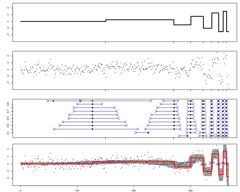
Figure 1. From top to bottom: 1. True regression function $\vartheta$. 2. Gaussian observations $Y$ with $n=367$ and variance $\sigma^{2}=1$. 3. Estimated change-point locations with confidence intervals for different values of $\alpha$ ($y$-axis). 4. SMUCE $\hat{\vartheta}(q_{\alpha})$ with confidence bands (gray hatched area) and confidence intervals for the change-point locations (inward pointed arrows) at $\alpha=0.4$.

1.2. Deviation bounds and confidence sets

The parameter $q\in\mathbb{R}$ in (2) plays a crucial role because it governs the trade-off between data-fit (the r.h.s. in (2)) and parsimony (the l.h.s. in (2)). It has an immediate statistical interpretation. From (2) it follows that

$$\mathbf{P}\left(\hat{K}(q)>K\right)\leq\mathbf{P}(T_{n}(Y,\vartheta)>q).$$ (7)

Hence, by choosing $q=q_{1-\alpha}$ to be the $1-\alpha$-quantile of the (asymptotic) null distribution of $T_{n}(Y,\vartheta)$, we can (asymptotically) control the probability of overestimating the number of change-points by $\alpha$. In fact, we show that the null distribution of $T_{n}(Y,\vartheta)$ can be bounded asymptotically by a distribution which does not depend on $\vartheta$ anymore (see Section 2.2). It is noteworthy that for Gaussian observations this bound is even non-asymptotic (see Section 2.4). The third panel in Figure 1 shows for different choices of $\alpha$ ($y$-axis) the corresponding estimates for the change-point locations (black dots; the vertical ticks mark the true change-point locations). The number of estimated change-points is monotonically increasing in $\alpha$ in accordance with (7) which guarantees at error level $\alpha$ that SMUCE has not more jumps than the true signal $\vartheta$. We emphasize that the SMUCE is remarkably stable w.r.t. the choice of $\alpha$, i.e. the number of change-points $K=8$ is estimated correctly for $0.2\leq\alpha\leq 0.9$. Our simulations in Section 5 confirm this stability even in non-Gaussian scenarios.

As mentioned before, the threshold $q_{1-\alpha}$ for SMUCE automatically controls the error of undersmoothing (7), i.e. the probability of overestimating the number of change-points. In addition, we prove an exponential inequality that bounds the error of oversmoothing, i.e. the probability of underestimating the number of change-points. Any such bound necessarily has to depend on the magnitude of the signal $\vartheta$ on the smallest scale, as no method can recover arbitrary fine details for given sample size $n$, see (Donoho, 1988) for a similar argument in the context of density estimation. Our bound (see Theorem 2.2)

$$\mathbf{P}\left(\hat{K}(q)<K\right)\leq 2Ke^{-Cn\lambda\Delta^{2}}\left[e^{\frac{1}{2}\left(q+\sqrt{2\log(2e/\lambda)}\right)^{2}}+e^{-3Cn\lambda\Delta^{2}}\right]$$ (8)

reflects this fact and indeed only depends on the smallest interval length $\lambda$, the smallest absolute jump size $\Delta$ and the number of change-points $K$ of the true regression function $\vartheta$. Here, $C>0$ is some known universal constant only depending on the family of distributions (see Section 2.3).

As a consequence of the inequalities (7) and (8), $\mathcal{C}(q_{1-\alpha})$ in (5) constitutes an asymptotic confidence set at level $1-\alpha$ and we will explain in Section 3.2 how confidence bands for the graph of $\vartheta$ and confidence intervals for its change-points can be obtained from this. See the lowest panel of Figure 1 for illustration.

Of course, honest (i.e. uniform) confidence sets cannot be obtained on the entire set of step functions $\mathcal{S}$, as $\Delta$ and $\lambda$ can become arbitrarily small. Nevertheless, we can show that simultaneously both, confidence bands for $\vartheta$ and intervals for the change-points are asymptotically honest w.r.t. to a sequence of nested models $\mathcal{S}^{(n)}\subset\mathcal{S}$ that satisfy

$$\frac{n}{\log n}\Delta_{n}^{2}\lambda_{n}\rightarrow\infty,\quad\text{ as }n\rightarrow\infty,$$ (9)

i.e. the confidence level $\alpha$ is kept uniformly over $\mathcal{S}^{(n)}$ as $n\rightarrow\infty$ (c.f. Section 2.6). Here $\lambda_{n}$ and $\Delta_{n}$ denote the smallest interval length and smallest absolute jump size in $\mathcal{S}^{(n)}$, respectively.

1.3. Choice of $q$

Balancing the probabilities for over- and underestimation in (7) and (8) gives an upper bound on $\mathbf{P}(\hat{K}(q)\neq K)$, the probability that the number of change-points is misspecified. This bound depends on $n,q,\lambda$ and $\Delta$ in an explicit way and opens the door for several strategies to select $q$, e.g. such that $\mathbf{P}(\hat{K}(q)=K)$ is maximized. One may additionally incorporate prior information on $\Delta$ and $\lambda$ and we suggest a simple way how to do this in Section 4.

A further consequence of (7) and (8) is that under a suitable choice of $q=q_{n}$ the probability of misspecification $\mathbf{P}(\hat{K}(q_{n})\neq K)$ tends to zero and hence $\hat{K}(q_{n})$ converges to the true number of change-points $K$ (model selection consistency), such that the underestimation error in (8) vanishes exponentially fast.

Finally, we obtain explicit bounds on the precision of estimating the change-point locations which again depend on $q,n,\lambda$ and $\Delta$. For any fixed $q>0$ they are recovered for all estimators in $\mathcal{C}(q)$, including SMUCE, at the optimal rate $1/n$ (up to a $\log$-factor). Moreover, these bounds can be used to derive slower rates uniformly over nested models as in (9) (see Section 2.6).

1.4. Detection power for vanishing signals

For the case of Gaussian observations we derive the detection power of the multiscale statistic $T_{n}$ in (3), i.e. we determine the maximal rate at which a signal may vanish with increasing $n$ but still can be detected with probability $1$, asymptotically. For the task of detecting a single constant signal against a noisy background, we obtain the optimal rate and constant (cf. (Dümbgen and Spokoiny, 2001; Dümbgen and Walther, 2008; Chan and Walther, 2013; Jeng et al., 2010)). We extend this result to the case of an arbitrary number of change-points, retrieving the same optimal rate but different constants (Section 2.5). Similar results have been derived recently in (Jeng et al., 2010) for sparse signals, where the estimator takes into account the explicit knowledge of sparsity. We stress that the SMUCE does not rely on any sparsity assumptions still it adapts automatically to sparse signals due to its multiscale nature.

1.5. Implementation, simulations and applications

The applicability of dynamic programming to the change-point problem has been subject of research recently (cf. e.g. (Boysen et al., 2009; Fearnhead, 2006; Friedrich et al., 2008; Harchaoui and Lévy-Leduc, 2010)). The SMUCE $\hat{\vartheta}(q)$ can also be computed by a dynamic program due to the restriction of the local likelihoods to the constant parts of candidate functions. This has already been observed by (Höhenrieder, 2008) for the multiscale constraint considered there. We prove that (6) can be rewritten into a minimization problem of a penalized cost function with a particular data driven penalty (see Lemma 3.1).

Much in the spirit of the dynamic program suggested in (Killick et al., 2011), our implementation exploits the structure of the constraint set in (6) to include pruning steps. These reduce the worst case computation time $\mathcal{O}(n^{2})$ considerably in practice and makes it applicable to large data sets. Simultaneously, the algorithm returns a confidence band for the graph of $\vartheta$ as well as confidence intervals for the location of the change-points (Section 3), the latter without any additional cost. An R-package (stepR) including an implementation of SMUCE is available online .

Extensive simulations reveal that the SMUCE is competitive with (and indeed often outperforms) state-of-the-art methods for the change-point problem which all have been tailor-made to specific exponential families (Section 5). Our simulation study includes the CBS method (Olshen et al., 2004), the fused lasso (Tibshirani et al., 2005) and the modified BIC (Zhang and Siegmund, 2007) for Gaussian regression, the multiscale estimator in (Davies et al., 2012) for piecewise constant volatility and the extended taut string method for quantile regression in (Dümbgen and Kovac, 2009). In our simulations we consider several risk measures, including the MSE and the model selection error $\mathbf{P}(\hat{K}\neq K)$. Moreover, we study the feasibility of our approach for different real-world data sets; including two benchmark examples from genetic engineering (Lai et al., 2005) and a new example from photoemission spectroscopy (Hüfner, 2003) which amounts to Poisson change-point regression. Finally, in Section 6, we briefly discuss possible extensions to serially dependent data, among others

1.6. Literature survey and connections to existing work

The problem of detecting changes in the characteristics of a sequence of observations has a long history in statistics and related fields, dating back to the 1950’s (see e.g.(Page, 1955)). In recent years, it experienced a renaissance in the context of regression analysis due to novel applications that mainly came along with the rapid development in genetic engineering (Braun et al., 2000; Olshen et al., 2004; Zhang and Siegmund, 2007; Jeng et al., 2010; Lebarbier and Picard, 2011) and financial econometrics (cf. (Inclán and Tiao, 1994; Lavielle and Teyssière, 2007; Davies et al., 2012; Spokoiny, 2009)). Due to the widespread occurrence of change-point problems in different communities and areas of applications, such as statistics (Carlstein et al., 1994), electrical engineering and signal processing (Blythe et al., 2012), mobile communication (Zhang et al., 2009), machine learning (Harchaoui and Lévy-Leduc, 2008), biophysics (Hotz et al., 2012), quantum optics (Schmidt et al., 2012), econometrics and quality control (Bai and Perron, 1998) and biology (Siegmund, 2013), an exhaustive list of existing methods is beyond reach. For a selective survey, we refer the reader also to the books (Brodsky and Darkhovsky, 1993; Csörgö and Horváth, 1997; Basseville and Nikiforov, 1993; Chen and Gupta, 2000; Wu, 2005) and the extensive list in (Khodadadi and Asgharian, 2008).

Our approach as outlined above can be considered as a hybrid method of two well-established approaches to the change-point problem:

Likelihood ratio and related statistics, on the one hand, are frequently employed to test for a change in the parameter of the distribution family and to construct confidence regions for change-point locations. Approaches of this type date back as far as (Chernoff and Zacks, 1964; Kander and Zacks, 1966) and have gained considerable attention afterwards (Hinkley, 1970; Hinkley and Hinkley, 1970; Hušková and Antoch, 2003; Worsley, 1983, 1986; Siegmund, 1988; Dümbgen, 1991) and (Bhattacharya, 1987; Siegmund and Yakir, 2000; Arias-Castro et al., 2011) for generalizations to the multivariate case). The likelihood ratio test was also extensively studied for sequential change-point analysis (Siegmund, 1986; Yakir and Pollak, 1998; Siegmund and Venkatraman, 1995). All these methods are primarily designed to detect a predefined maximal number (mostly one) of change-points.

On the other hand, if the number of change-points is unknown, an additional model selection step is required, which can be achieved by proper penalization of model complexity, e.g. measured by the number of change-points itself or by surrogates for it. This is often approached by maximizing a penalized likelihood function of the form

$$\vartheta\mapsto l(Y,\vartheta)-\text{pen}(\vartheta)$$

over a suitable space of functions, e.g. $\mathcal{S}$ as in this paper or functions of bounded variation (Mammen and van de Geer, 1997), etc. Here $l(Y,\vartheta)$ is the (log) likelihood function. The penalty term $\text{pen}(\vartheta)$ penalizes the complexity of $\vartheta$ and prevents overfitting. It increases with the dimension of the model and serves as a model selection criterion. First approaches include BIC-type penalties (Yao, 1988) and more sophisticated penalties have been advocated later on (see e.g. (Yao and Au, 1989; Lavielle and Moulines, 2000; Braun et al., 2000; Birgé and Massart, 2001; Lavielle, 2005; Lavielle and Teyssière, 2007; Boysen et al., 2009; Arlot et al., 2012; Wittich et al., 2008; Winkler and Liebscher, 2002)). Further prominent penalization approaches include the fused lasso procedure (see (Friedman et al., 2007; Tibshirani et al., 2005) and (Harchaoui and Lévy-Leduc, 2010)) that uses a linear combination of the total-variation and the $\ell^{1}$-norm penalty as a convex surrogate for the number of change-points which has been primarily designed for the situation when $\vartheta$ is sparse. Recently, aggregation methods (Rigollet and Tsybakov, 2012) have been advocated recently for the change-point regression problem as well.

Most similar in spirit to our approach are estimators which minimize target functionals under a statistical multiscale constraint. For some early references see (Nemirovski, 1985; Donoho, 1995) and more recently (Davies et al., 2009; Candes and Tao, 2007; Frick et al., 2012; Davies and Kovac, 2001). In our case this target functional equals the number of change-points.

The multiscale calibration in (3) is based on the work of (Dümbgen and Spokoiny, 2001; Dümbgen and Walther, 2008; Chan and Walther, 2013). Multiscale penalization methods have been suggested in (Zhang and Siegmund, 2007; Kolaczyk and Nowak, 2004), multiscale partitioning methods including binary segmentation in (Sen and Srivastava, 1975; Vostrikova, 1981; Olshen et al., 2004; Fryzlewicz, 2012), and recursive partitioning in (Kolaczyk and Nowak, 2005).

Aside to the connection to frequentist’s work cited above, we claim that our analysis also provides an interface for incorporating a priori information on the true signal into the estimator (see Section 4). We stress that for minimizing the bounds in (7) and (8) on the model selection error $\mathbf{P}(\hat{K}(q)\neq K)$ it is not necessary to include full priors on the space of step functions $\mathcal{S}$. Instead it suffices to simply specify a prior on the smallest interval length $\lambda$ and the smallest absolute jump size $\Delta$. The parameter choice strategy discussed in Section 4 or the limiting distribution of $T_{n}(Y,\vartheta)$ in Section 2.2, for instance, can be refined within such a Bayesian framework. This, however, will not be discussed in this paper in detail and is postponed to future work. For recent work on a Bayesian approach to the change-point problem we refer to (Du and Kou, 2012; Fearnhead, 2006; Luong et al., 2012; Rigaill et al., 2012) and the references therein.

We finally stress that there is a conceptual analogy of SMUCE to the Dantzig selector as introduced in (Candes and Tao, 2007) for estimating sparse signals in gaussian high dimensional linear regression models (see (James and Radchenko, 2009) for an extension to exponential families). Here the $\ell_{1}$-norm of the signal is to be minimized subject to the constraint that the residuals are pointwise within the noise level. The SMUCE, in contrast, minimizes the $\ell_{0}$-norm of the discrete derivative of the signal subject to the constraint that the residuals are tested to contain no signal on all scales. We will briefly address this and other relations to recent concepts in high dimensional statistics in a discussion in Section 6. In summary, the change-point problem is an “$n=p$” problem and hence substantially different from high dimensional regression where “$p\gg n$”. As we will show, multiscale detection of sparse signals becomes then possible without any sparsity assumption entering the estimator. Another major statistical consequence of this paper is that post model selection inference is doable over a large range of scales uniformly over nested models in the sense of (9).

2. Theory

This section summarizes our main theoretical findings. In Section 2.3 we discuss consistency of the estimated number of change-points. This result follows from an exponential bound for the probability of underestimating the number of change-points on the one hand. On the other hand we show how to control the probability of overestimating the number of change-points by means of the limiting distribution of $T_{n}(Y,\vartheta)$ as $n\rightarrow\infty$ (cf. Section 2.2). We give improved results, including a non-asymptotic bound for the probability of overestimating the number of change-points, for Gaussian observations (cf. Sections 2.4 & 2.5). In Section 2.6 we finally show that the change-point locations can be recovered as fast as the sampling rate up to a $\log$-factor and discuss how asymptotically honest confidence sets for $\vartheta$ can be constructed over a suitable sequence of nested models.

2.1. Notation and model

We shall henceforth assume that $\mathcal{F}=\left\{F_{\theta}\right\}_{\theta\in\Theta}$ is a one-dimensional, standard exponential family with $\nu$-densities

$$f_{\theta}(x)=\exp\left(\theta x-\psi(\theta)\right),\quad x\in\mathbb{R}.$$ (10)

Here $\Theta=\left\{\theta\in\mathbb{R}~{}:~{}\int_{\mathbb{R}}\exp(\theta x)\textnormal{\,d}\nu(x)<\infty\right\}\subseteq\mathbb{R}$ denotes the natural parameter space. We will assume that $\mathcal{F}$ is regular and minimal which means that $\Theta$ is an open interval and that the cumulant transform $\psi$ is strictly convex on $\Theta$. We will frequently make use of the functions

$$m(\theta):=\dot{\psi}(\theta)=\mathbf{E}\left(X\right)\quad\text{ and }\quad v(\theta):=\ddot{\psi}(\theta)=\mathbf{Var}\left(X\right),$$ (11)

for $X\sim F_{\theta}$. Note that $m$ and $v$ are strictly increasing and positive on $\Theta$, respectively.

2.1.1. Observation model and step functions

We assume that $Y=(Y_{1},\ldots,Y_{n})$ are independent observations given by (1) where $\vartheta:[0,1)\rightarrow\Theta$ is a right continuous step function, that is

$$\vartheta(t)=\sum_{k=0}^{K}\theta_{k}\mathbf{1}_{[\tau_{k},\tau_{k+1})}(t),$$ (12)

where $0=\tau_{0}<\tau_{1}<\ldots<\tau_{K}<\tau_{K+1}=1$ are the change-point locations and $\theta_{k}\in\Theta$ the corresponding intensities, such that $\theta_{k}\neq\theta_{k+1}$ for $k=0,\ldots,K$. The collection of step functions on $[0,1)$ with values in $\Theta$ and an arbitrary but finite number of change-points will be denoted by $\mathcal{S}$. For $\vartheta\in\mathcal{S}$ as in (12) we denote by $J(\vartheta)=(\tau_{1},\ldots,\tau_{K})$ the increasingly ordered vector of change-points and by $\#J(\vartheta)=K\in\mathbb{N}$ its length. We will denote the set of step functions with $K$ change-points and change-point locations restricted to the sample grid by $\mathcal{S}_{n}[K]\subset\mathcal{S}$.

For any estimator $\hat{\vartheta}$ of $\vartheta\in\mathcal{S}$, the estimated number of change-points will be denoted by $\#J(\hat{\vartheta})=\hat{K}$, the change-point locations by $J(\hat{\vartheta})=(\hat{\tau}_{1},\ldots,\hat{\tau}_{\hat{K}})$ and we set $\hat{\theta}_{k}=\hat{\vartheta}(t)$ for $t\in[\hat{\tau}_{k},\hat{\tau}_{k+1})$. For simplicity, for each $n\in\mathbb{N}$ we restrict to estimators which have change-points only at sampling points, i.e. $\hat{\vartheta}\in\mathcal{S}_{n}[K]$ with $\hat{\tau}_{k}=\hat{l}_{k}/n$ for some $1\leq\hat{l}_{k}\leq n$. To keep the presentation simple, throughout the following we restrict ourselves to an equidistant sampling scheme as in (1). However, we mention that extensions to more general designs are possible.

2.1.2. Multiscale statistic

Let $1\leq i\leq j\leq n$. Then, the likelihood ratio statistic $T_{i}^{j}(Y,\theta)$ in (4) can be rewritten into

$$T_{i}^{j}(Y,\theta_{0})=\sup_{\theta\in\Theta}\left(\sum_{l=i}^{j}(\theta Y_{l}-\psi(\theta))\right)-\sum_{l=i}^{j}(\theta_{0}Y_{l}-\psi(\theta_{0})).$$

Introducing the notation $\phi(x)=\sup_{\theta\in\Theta}\theta x-\psi(\theta)$ for the Legendre-Fenchel conjugate of $\psi$ and $J(x,\theta)=\phi(x)-(\theta x-\psi(\theta))$ we find

$$T_{i}^{j}(Y,\theta_{0})=(j-i+1)J(\overline{Y}_{i}^{j},\theta_{0})\geq 0,$$

where $\overline{Y}_{i}^{j}=(\sum_{i\leq l\leq j}Y_{l})/(j-i+1)$. The multiscale statistic $T_{n}(Y,\vartheta)$ in (3) was defined to be the (scale calibrated) maximum over all $\sqrt{2T_{i}^{j}}$ such that $\hat{l}_{k}\leq i\leq j<\hat{l}_{k+1}$ for some $0\leq k\leq\hat{K}$. As mentioned in the introduction we sometimes will restrict the minimal interval length (scale) by a sequence of lower bounds $(c_{n})_{n\in\mathbb{N}}$ tending to zero. In order to ensure that the asymptotic null distribution is non degenerate, we assume for non-Gaussian families (see also (Schmidt-Hieber et al., 2011))

$$n^{-1}\log^{3}n/c_{n}\rightarrow 0.$$ (13)

Then, the modified version of (3) reads as

$$T_{n}(Y,\vartheta;c_{n})=\max_{0\leq k\leq{K}}\max_{\begin{subarray}{c}l_{k}\leq i\leq j<l_{k+1}\\ (j-i+1)/n\geq c_{n}\end{subarray}}\left(\sqrt{2T_{i}^{j}(Y,\theta_{k})}-\sqrt{2\log\frac{ne}{j-i+1}}\right).$$ (14)

2.2. Asymptotic null distribution

We give a representation of the limiting distribution of the multiscale statistic $T_{n}$ in (14) in terms of

$$M:=\sup_{0\leq s<t\leq 1}\left(\frac{\left|B(t)-B(s)\right|}{\sqrt{t-s}}-\sqrt{2\log\frac{e}{t-s}}\right),$$ (15)

where $(B(t))_{t\geq 0}$ denotes a standard Brownian motion. We stress that the statistic $M$ is finite almost surely and has a continuous distribution supported on $[0,\infty)$ (cf. (Dümbgen and Spokoiny, 2001; Dümbgen et al., 2006)).

Theorem 2.1.

Assume that $(c_{n})_{n\in\mathbb{N}}$ satisfies (13). Then,

$$T_{n}(Y,\vartheta;c_{n})\stackrel{{\scriptstyle D}}{{\rightarrow}}\max_{0\leq k\leq K}\sup_{\tau_{k}\leq s<t\leq\tau_{k+1}}\left(\frac{\left|B(t)-B(s)\right|}{\sqrt{t-s}}-\sqrt{2\log\frac{e}{t-s}}\right).$$ (16)

Further, let $M_{0},\ldots,M_{K}$ be independent copies of $M$ as in (15). Then, the right hand side in (16) is stochastically bounded from above by $M$ and from below by

$$\max_{0\leq k\leq K}\left(M_{k}-\sqrt{2\log\frac{1}{\tau_{k+1}-\tau_{k}}}\right).$$

It is important to note that the limit distribution in (16) (same as the lower bound) depends on the unknown regression function $\vartheta$ only through the number of change-points $K$ and the change-point locations $\tau_{k}$, i.e. the function values of $\vartheta$ do not play a role. From the upper bound in Theorem 2.1 we obtain

$$\lim_{n\rightarrow\infty}\mathbf{P}\left(T_{n}(Y,\vartheta;c_{n})\leq q_{\alpha}\right)\geq\alpha,$$ (17)

with $q_{\alpha}$ being the $\alpha$-quantile of $M$. In practice the distribution of $M$ is obtained by simulations. In Section 2.4 we will see that for the Gaussian case even a nonasymptotic version of Theorem 2.1 can be obtained, which allows for finite sample refinement of the null distribution of $T_{n}$. As the asymptotics is rather slow, this finite sample correction is helpful even for relatively large samples, say if $n$ is of the order of a few thousands. This is highlighted in Figure 2 where it becomes apparent that the empirical null distributions for finite samples, obtained from simulations, is in general not supported in $[0,\infty)$.

Figure 2. Simulations of the cdf (left) and density (right) of $M$ as in (15) for $n=50$(dotted line), $n=500$(dashed line) and $n=5000$(solid line) equidistant discretization points.

To the best of our knowledge, it is an open and challenging problem to derive tight bounds for the tails of $M$ (cf. (Dümbgen and Spokoiny, 2001; Dümbgen and Walther, 2008; Dümbgen et al., 2006)) which is not addressed in this article. By such bounds the probability of overestimating the number of change-points could be controlled explicitly, as we will see in the upcoming section. Moreover, we point out that the inequality in (17) is not sharp, if the true functions has at least one change-point. This is due to the fact that we bound $T_{n}$ in (17) by $q_{\alpha}$, the quantile of $M$ which serves as the bound for the r.h.s. in (16). For an illustration of this, Figure 3 shows P-P plots of the exact null distribution of signals with $2$, $4$ and $10$ equidistant change-points against the null distribution of a signal without change-points for sample size $n=500$. Of course, further information on the minimal number and location of change-points can be used to improve the distributional bound by $M$ in Theorem 2.1. We will not pursue this further.

Figure 3. Probability-Probability plots of the empirical null distribution of a signal without change-points ($x$-axis) against signals with $2$(left), $5$(middle) and $10$(right) equidistant change-points ($y$-axis) for $n=500$.

2.3. Exponential inequality for the estimated number of change-points

In this section we derive explicit bounds on the probability that $\hat{K}(q)$ as defined in (2) underestimates the true number of change-points $K$. In combination with the results in Section 2.2, these bounds will imply model selection consistency, i.e. $\mathbf{P}(\hat{K}(q_{n})=K)\rightarrow 1$ for a suitable sequence of thresholds $(q_{n})_{n\in\mathbb{N}}$ in (2).

We first note, that with the additional constraint in (14) on the minimal interval length, the estimated number of change-points is given by

$$\hat{K}(q)=\min\left\{K\in\mathbb{N}~{}:~{}\exists\vartheta\in\mathcal{S}_{n}[K]:T_{n}(Y,\vartheta;c_{n})\leq q\right\},\quad q\in\mathbb{R}.$$ (18)

Now let $\Delta$ and $\lambda$ be the smallest absolute jump size and the smallest interval length of the true regression function $\vartheta\in\mathcal{S}$, respectively and assume that $\vartheta(t)\in[\underline{\theta},\overline{\theta}]$ for all $t\in[0,1]$. We give the aforementioned exponential upper bound on the probability that the number of change-points is underestimated. The results follows from the general exponential inequality in the supplement, Theorem 7.10.

Theorem 2.2 (Underestimation bound).

Let $q\in\mathbb{R}$ and $\hat{K}(q)$ be defined as in (18) with $\lambda\geq 2c_{n}$. Then, there exists a constant $C=C(\mathcal{F},\underline{\theta},\overline{\theta})>0$ s.t.

$$\mathbf{P}\left(\hat{K}(q)<K\right)\leq 2Ke^{-Cn\lambda\Delta^{2}}\left[e^{\frac{1}{2}\left(q+\sqrt{2\log(2e/\lambda)}\right)^{2}}+e^{-3Cn\lambda\Delta^{2}}\right],\quad n\in\mathbb{N}.$$ (19)

From Theorem 7.10 and Lemma 7.11 it follows that

$$C(\mathcal{F},\underline{\theta},\overline{\theta})=\frac{1}{32}\frac{\inf_{\underline{\theta}\leq\theta\leq\overline{\theta}}v(t)^{2}}{\sup_{\underline{\theta}\leq\theta\leq\overline{\theta}}v(t)},$$ (20)

which gives $C=1/32$ for the Gaussian family and $C=\underline{\mu}^{2}/(32\overline{\mu})$ for the Poisson family, given $m(\vartheta)\in[\underline{\mu},\overline{\mu}]$ in the latter case.

On the one hand, if $q=q_{n}$ and $q_{n}/\sqrt{n}\rightarrow 0$ as $n\rightarrow\infty$, it becomes clear from Theorem 2.2 that $\hat{K}(q_{n})\geq K$ with high probability. On the other hand, it follows from Theorem 2.1 that $T_{n}(Y,\vartheta;c_{n})$ is bounded almost surely as $n\rightarrow\infty$ if $c_{n}$ is as in (13). This in turn implies that the probability for $\hat{K}(q_{n})\leq K$ tends to $1$, since

$$\mathbf{P}\left(\hat{K}(q_{n})>K\right)\leq\mathbf{P}(T_{n}(Y,\vartheta;c_{n})>q_{n})\rightarrow 0,$$ (21)

whenever $q_{n}\rightarrow\infty$, as $n\rightarrow\infty$. Thus, we summarize

Theorem 2.3 (Model selection consistency).

Let the assumptions of Theorems 2.1 and 2.2 hold and additionally assume that $q_{n}\rightarrow\infty$ and $q_{n}/\sqrt{n}\rightarrow 0$ as $n\rightarrow\infty$. Then,

$$\lim_{n\rightarrow\infty}\mathbf{P}(\hat{K}(q_{n})=K)=1.$$

Giving a non-asymptotic bound for the probability for overestimating the true number of change-points (in the spirit of (21)) appears to be rather difficult in general. For the Gaussian case though this is possible, as we will show in the next section.

2.4. Gaussian observations

We now derive sharper results for the case when $\mathcal{F}$ is the Gaussian family of distributions with constant variance. In this case (1) reads as

$$Y_{i}=\mu(i/n)+\sigma\varepsilon_{i},\quad i=1,\ldots,n$$ (22)

where $\varepsilon_{1},\ldots,\varepsilon_{n}$ are independent $\mathcal{N}(0,1)$ random variables, $\sigma>0$ and $\mu\in\mathcal{S}$ denotes the expectation of $Y$. To ease notation we assume in the following that $\sigma=1$. For the general case replace $\Delta$ by $\Delta/\sigma$.

In the Gaussian case it is possible to get rid of the lower bound for the smallest scales $c_{n}$ as in (13) because the strong approximation by Gaussian observations in the proof of Theorem 2.1 becomes superfluous. We obtain the following non-asymptotic result on the null distribution.

Theorem 2.4 (Null Distribution of $T_{n}$).

For any $n\in\mathbb{N}$

$$\max_{0\leq k\leq K}\left(M_{k}-\sqrt{2\log\frac{1}{\tau_{k+1}-\tau_{k}}}\right)\stackrel{{\scriptstyle\mathcal{D}}}{{\leq}}T_{n}(Y,\vartheta)\stackrel{{\scriptstyle\mathcal{D}}}{{\leq}}M^{(n)}\stackrel{{\scriptstyle\mathcal{D}}}{{\leq}}M,$$

where $M^{(n)}$ is as $M$ in (15) where the supremum is only taken over the system of discrete intervals $[i/n,j/n]$.

In contrast to Theorem 2.1, this result is nonasymptotic and the inequality holds for any sample size. For this reason, we get the following improved upper bound for the probability of overestimating the number of change-points.

Corollary 2.5 (Overestimation bound).

Let $q\in\mathbb{R}$ and $\hat{K}(q)$ be defined as in (18). Then for any $n\in\mathbb{N}$

$$\mathbf{P}\left(\hat{K}(q)>K\right)\leq\mathbf{P}\left(M\geq q\right).$$

This corresponds to the “worst case scenario” for overestimation when the true signal $\vartheta$ has no jump.

For the probability of underestimating the number of change-points, we can improve Theorem 2.2 for Gaussian observations (see Theorem 7.12) to

$$\mathbf{P}\left(\hat{K}(q)<K\right)\leq 2K\left[\exp\left(-\frac{1}{8}\left(\frac{\Delta\sqrt{\lambda n}}{2\sqrt{2}}-q-\sqrt{2\log\frac{2e}{\lambda}}\right)_{+}^{2}\right)+\exp\left(-\frac{\lambda n\Delta^{2}}{16}\right)\right].$$ (23)

2.5. Multiscale detection of vanishing signals for Gaussian observations

We will now discuss the ability of SMUCE to detect vanishing changes in a signal. We begin with the problem of detecting a signal on a single interval against an unknown background.

Theorem 2.6.

Let $\vartheta_{n}(t)=\theta_{0}+\delta_{n}I_{n}(t)$ for some $\theta_{0},\theta_{0}+\delta_{n}\in\Theta$ and for some sequence of intervals $I_{n}\subset[0,1]$ and $Y$ be given by (22). Further let $(q_{n})_{n\in\mathbb{N}}$ be bounded away from zero and assume

1. for signals on a large scale (i.e. $\liminf\left|I_{n}\right|>0$), that $\sqrt{\left|I_{n}\right|n}\delta_{n}/{q_{n}}\rightarrow\infty$,

2. for signals on a small scale (i.e. $\left|I_{n}\right|\rightarrow 0$), that $\sqrt{\left|I_{n}\right|n}\delta_{n}\geq(\sqrt{2}+\varepsilon_{n})\sqrt{\log(1/\left|I_{n}\right|)}$ with $\varepsilon_{n}$, s.t. $\varepsilon_{n}\sqrt{\log(1/\left|I_{n}\right|)}\rightarrow\infty$ and $\sup_{n\in\mathbb{N}}q_{n}/(\varepsilon_{n}\sqrt{\log(1/\left|I_{n}\right|)})<1$.

Then,

$$\sup_{\vartheta_{0}\equiv\theta\in\Theta}\mathbf{P}_{\vartheta_{n}}\left(T_{n}(Y,\vartheta_{0})\leq q_{n}\right)\rightarrow 0.$$ (24)

Theorem 2.6 gives sufficient conditions on the signals $\vartheta_{n}$ (through the interval length $\left|I_{n}\right|$ and the jump height $\delta_{n}$) as well as on the thresholds $q_{n}$ such that the multiscale

statistic $T_{n}$ detects the signals with probability $1$, asymptotically; put differently, this means $\mathbf{P}(\hat{K}(q_{n})>0)\rightarrow 1$. We stress that the above result is optimal in the following sense: No test can detect signals satisfying $\sqrt{\left|I_{n}\right|n}\delta\geq(\sqrt{2}-\varepsilon_{n})\sqrt{\log(1/I_{n})}$ with asymptotic power $1$ (see (Dümbgen and Spokoiny, 2001; Chan and Walther, 2013; Jeng et al., 2010)).

For the special case, when $q_{n}\equiv q_{\alpha}$ is a fixed $\alpha$-quantile of the null distribution $T_{n}(Y,\vartheta_{n})$ (or of the limiting distribution $M$ in (15)), the result boils down to the findings in (Dümbgen and Spokoiny, 2001; Chan and Walther, 2013). In particular, aside to the optimal asymptotic power (24), the error of first kind is bounded by $\alpha$. The result in Theorem 2.6 goes beyond that and allows to shrink the error of first kind to zero asymptotically, by choosing $q_{n}\rightarrow\infty$.

We finally generalize the results in Theorem 2.6 to the case when $\vartheta\in\mathcal{S}$ has more than one change-point. To be more precise, we formulate conditions on the smallest interval and the smallest jump in $\vartheta$ such that no change-point is missed asymptotically.

Theorem 2.7.

Let $(\vartheta_{n})_{n\in\mathbb{N}}$ be a sequence in $\mathcal{S}$ with $K_{n}$ change-points and denote by $\Delta_{n}$ and $\lambda_{n}$ the smallest absolute jump size and smallest interval in $\vartheta_{n}$, respectively. Further, assume that $q_{n}$ is bounded away from zero and

1. for signals on large scales (i.e. $\liminf\lambda_{n}>0$), that $\sqrt{\lambda_{n}n}\Delta_{n}/q_{n}\rightarrow\infty$.

2. for signals on small scales (i.e. $\lambda_{n}\rightarrow 0$) with $K_{n}$ bounded, that $\sqrt{\lambda_{n}n}\Delta_{n}\geq(4+\varepsilon_{n})\sqrt{\log(1/\lambda_{n})}$ with $\varepsilon_{n}\sqrt{\log(1/\lambda_{n})}\rightarrow\infty$ and $\sup_{n\in\mathbb{N}}q_{n}/(\varepsilon_{n}\sqrt{\log(1/\lambda_{n})})<{1/(2\sqrt{2})}$.

3. the same as in (2), with $K_{n}$ unbounded and the constant $12$ instead of $4$.

Then,

$$\mathbf{P}_{\vartheta_{n}}\left(\hat{K}(q_{n})\geq K_{n}\right)\rightarrow 1.$$

Theorem 2.7 amounts to say that the statistic $T_{n}$ is capable of detecting multiple change-points simultaneously at the same optimal rate (in terms of the smallest interval and jump) as a single change-point. The only difference being the constants that bound the size of the signals that can be detected. These increase with the complexity of the problem: $\sqrt{2}$ for a single change against an unknown background, $4$ for a bounded (but unknown), and $12$ for an unbounded number of change-points. In (Jeng et al., 2010) it was shown that for step functions that exhibit certain sparsity patterns the optimal constant $\sqrt{2}$ can be achieved. It is important to note that we do not make any sparsity assumption on the true signal. Finally we mention an analogy to Theorem 4.1. of (Dümbgen and Walther, 2008) in the context of detecting local increases and decreases of a density. As in Theorem 2.7 only the constants and not the detection rates changes with the complexity of the alternatives.

2.6. Estimation of change-point locations and simultaneous confidence sets

In this section we will provide several results on confidence sets associated with SMUCE. We will see that these are linked in a natural way to estimation of change-point locations. We generalize the set $\mathcal{C}(q)$ in (5) by replacing $T_{n}(Y,\vartheta)$ in (3) with $T_{n}(Y,\vartheta,c_{n})$ as in (14) and consider the set of solutions of the optimization problem

$$\inf_{\vartheta\in\mathcal{S}}\#J(\vartheta)\quad\text{ s.t. }\quad T_{n}(Y,\vartheta;c_{n})\leq q.$$ (25)

Any candidate in $\mathcal{C}(q)$ recovers the change-point locations of the true regression function $\vartheta$ with the same convergence rate. It is determined by the smallest scale $(c_{n})_{n\in\mathbb{N}}$ for the considered interval lengths in the multiscale statistic $T_{n}$ in (14) and hence equals the sampling rate up to a log factor.

Theorem 2.8.

Let $q\in\mathbb{R}$ and $\mathcal{C}(q)$ be the set of solutions of (25) and $(c_{n})_{n\in\mathbb{N}}$ a sequence in $(0,1]$. Further let $C=C(\mathcal{F},\underline{\theta},\overline{\theta})>0$ as in (20). Then, for all $n\in\mathbb{N}$

$$\mathbf{P}\left(\sup_{\hat{\vartheta}\in\mathcal{C}(q)}{\max_{\tau\in J(\vartheta)}\min_{\hat{\tau}\in J(\hat{\vartheta})}}\left|\hat{\tau}-\tau\right|>c_{n}\right)\leq 2Ke^{-2Cnc_{n}\Delta^{2}}\left[e^{\frac{1}{2}\left(q+\sqrt{2\log(e/c_{n})}\right)^{2}}+e^{-{6}Cnc_{n}\Delta^{2}}\right].$$

For a fixed signal $\vartheta\in\mathcal{S}$, a sufficient condition for the r.h.s. in Theorem 2.8 to vanish as $n\rightarrow\infty$ is

$$c_{n}\geq\frac{1}{\Delta^{2}C}\frac{\log{n}}{n}.$$

Here the constant $C$ matters, e.g. in the Gaussian case $C=1/8$ (cf. Section 2.3). This improves several results obtained for other methods, e.g. in (Harchaoui and Lévy-Leduc, 2010) for a total variation penalized estimator a $\log^{2}{n}/n$ rate has been shown.

In the following we will apply Theorem 2.8 to determine subclasses of $\mathcal{S}$ in which the change-point locations are reconstructed uniformly with rate $c_{n}$. These subclasses are delimited by conditions on the smallest absolute jump height $\Delta_{n}$ and on the number of change-points $K_{n}$ (or the smallest interval lengths $\lambda_{n}$ by using the relation $K_{n}\leq 1/\lambda_{n}$) of its members. For instance, the rate function $c_{n}=n^{-\beta}$ with some $\beta\in[0,1)$ implies the condition

$$\frac{n^{\beta}\exp(-n^{1-\beta}\Delta_{n})}{\lambda_{n}}\rightarrow 0.$$

The choice $\beta=0$ gives the largest subclass but no convergence rate is guaranteed since $c_{n}=1$ for all $n$. A value of $\beta$ close to $1$ implies a much smaller subclass of functions which then can be reconstructed uniformly with convergence rate arbitrarily close to the sampling rate $1/n$. We finally point out that the result in Theorem 2.8 does not presume the number of change-points to be estimated correctly. If $c_{n}$ additionally satisfies (13) and if in Theorem (2.8) $q=q_{n}\rightarrow\infty$ slower than $-\log c_{n}$, we find from Theorem 2.3 that $\mathbf{P}(\hat{K}(q)=K)\rightarrow 1$ and it follows from Theorem (2.8) that for $n$ large enough

$$\mathbf{P}\left(\sup_{\hat{\vartheta}\in\mathcal{C}(q_{n})}c_{n}^{-1}\left|\tau_{k}-\hat{\tau}_{k}\right|>1\right)\rightarrow 0,\quad\text{for }k=1,\dots,K.$$

The solution set of the optimization problem (25) constitutes a confidence set for the true regression function $\vartheta$. Indeed, we find that

$$\mathbf{P}\left(\vartheta\in\mathcal{C}(q)\right) =\mathbf{P}\left(T_{n}(Y,\vartheta;c_{n})\leq q,\;K\leq\hat{K}(q)\right)$$ (26)

$$\geq\mathbf{P}\left(T_{n}(Y,\vartheta;c_{n})\leq q\right)-\mathbf{P}\left(\hat{K}(q)<K\right).$$

In particular, it follows from Theorem 2.3 that if $q_{1-\alpha}$ is the $1-\alpha$-quantile of $M$, the set $\mathcal{C}(q_{1-\alpha})$ is an asymptotic confidence set at level $1-\alpha$.

Corollary 2.9.

Let $\alpha\in(0,1)$ and $q_{1-\alpha}$ to be the $1-\alpha$-quantile of the statistic $M$ in (15). Then,

$$\mathbf{P}\left(\vartheta\in\mathcal{C}(q_{1-\alpha})\right)\geq 1-\alpha-2Ke^{-Cn\lambda\Delta^{2}}\left[e^{\frac{1}{2}\left({q_{1-\alpha}}+\sqrt{2\log(2e/\lambda)}\right)^{2}}+e^{-{3}Cn\lambda\Delta^{2}}\right]+\textnormal{o}(1)$$ (27)

with $C=C(\mathcal{F},\underline{\theta},\overline{\theta})>0$ as in Theorem 2.3. Consequently one finds

$$\lim_{n\rightarrow\infty}\mathbf{P}\left(\vartheta\in\mathcal{C}(q_{1-\alpha})\right)\geq 1-\alpha.$$

for any $\vartheta\in\mathcal{S}$.

We mention that for the Gaussian family (see Section 2.4) the inequality (27) even holds for any $n$, i.e. the $\textnormal{o}(1)$ term on the r.h.s. can be omitted. Thus the r.h.s. of (27) gives an explicit and nonasymptotic lower bound for the true confidence level of $C(q_{\alpha})$.

In the following we use this result to determine classes of step functions on which confidence statements hold uniformly. Being a subset of $\mathcal{S}$, the confidence set $\mathcal{C}(q)$ is hard to visualize in practice. Therefore, in Section 3.2 we compute a confidence band $B(q)\subset[0,1]\times\Theta$ that contains the graphs of all functions in $\mathcal{C}(q)$ as well as disjoint confidence intervals for the change-point locations denoted by $[\tau_{k}^{l}(q),\tau_{k}^{r}(q)]\subset[0,1]$ for $k=1,\ldots,\hat{K}(q)$. For the sake of simplicity, we denote the collection $\{\hat{K}(q),B(q),\left\{[\tau_{k}^{l}(q),\tau_{k}^{r}(q)]\right\}_{k=1,\ldots,\hat{K}(q)}\}$ by $I(q)$ and agree upon the notation

$$\vartheta\prec I(q)\quad \text{if }\hat{K}(q)=K,(t,\vartheta(t))\in B(q)\text{ and }\tau_{k}\in[\tau_{k}^{l}(q),\tau_{k}^{r}(q)]\text{ for }k=1,\ldots,K,$$ (28)

$$\vartheta\nprec I(q)\quad \text{otherwise}.$$

Put differently, $\vartheta\prec I(q)$ implies that simultaneously the number of change-points is estimated correctly, the change-points lie within the confidence intervals and the graph is contained in the confidence band. As we will show in Section 3.2, the confidence set $\mathcal{C}(q)$ and $I(q)$ are linked by the following relation:

$$\vartheta\in\mathcal{C}(q)\Rightarrow\vartheta\prec I(q).$$ (29)

Following the terminology in (Li, 1989), $I(q)$ is called asymptotically honest for the class $\mathcal{S}$ at level $1-\alpha$ if

$$\liminf_{n\rightarrow\infty}\inf_{\vartheta\in\mathcal{S}}\mathbf{P}\left(\vartheta\prec I(q)\right)\geq 1-\alpha.$$

Such a condition obviously cannot be fulfilled over the entire class $\mathcal{S}$, since signals cannot be detected if they vanish too fast as $n\rightarrow\infty$. For Gaussian observations this was made precise in Section 2.4.

To overcome this difficulty, we will relax the notion of asymptotic honesty. Let $\mathcal{S}^{(n)}\subset\mathcal{S}$, $n\in\mathbb{N}$ be a sequence of subclasses of $\mathcal{S}$. Then $I(q)$ is sequentially honest w.r.t. $S^{(n)}$ at level $1-\alpha$ if

$$\liminf_{n\rightarrow\infty}\inf_{\vartheta\in\mathcal{S}^{(n)}}\mathbf{P}\left(\vartheta\prec I(q)\right)\geq 1-\alpha.$$

By combining (26), (29) and Corollary 2.2 we obtain the following result about the asymptotic honesty of $I(q_{1-\alpha})$.

Corollary 2.10.

Let $\alpha\in(0,1)$ and $q_{1-\alpha}$ be the $1-\alpha$-quantile of the statistic $M$ in (15) and assume that $(b_{n})_{n\in\mathbb{N}}\rightarrow\infty$ is a sequence of positive numbers. Define $\mathcal{S}^{(n)}=\left\{\vartheta\in\mathcal{S}:n\lambda\Delta^{2}/\log(1/\lambda)\geq b_{n},\;\underline{\theta}\leq\vartheta\leq\overline{\theta}\right\}$. Then $I(q_{1-\alpha})$ is sequentially honest w.r.t. $\mathcal{S}^{(n)}$ at level $1-\alpha$, i.e.

$$\lim_{n\rightarrow\infty}\inf_{\vartheta\in\mathcal{S}^{(n)}}\mathbf{P}\left(\vartheta\prec I(q_{{1-\alpha}})\right)\geq 1-\alpha.$$

By estimating $1/\lambda\leq n$ we find that the confidence level $\alpha$ is kept uniformly over nested models $\mathcal{S}^{(n)}\subset\mathcal{S}$, as long as $\frac{n}{\log n}\Delta_{n}^{2}\lambda_{n}\rightarrow\infty$. Here $\lambda_{n}$ and $\Delta_{n}$ is the smallest interval length and smallest absolute jump size in $\mathcal{S}^{(n)}$, respectively.

3. Implementation

We now explain how the SMUCE, i.e. the estimator $\hat{\vartheta}(q)$ with maximal likelihood in the confidence set $\mathcal{C}(q)$, can be computed efficiently within the dynamic programming framework. In general the proposed algorithm is of complexity $\mathcal{O}(n^{2})$. We will show, however, that in many situations the computation can be performed much faster.

Our algorithm uses dynamic programming ideas from (Friedrich et al., 2008) in the context of complexity penalized M-estimation. See also (Höhenrieder, 2008; Davies et al., 2012) for a special case in our context. Moreover, we include pruning steps as (Killick et al., 2011), who also provide a survey on dynamic programming in change-point regression from a general point of view. We will show that it is always possible to rewrite $\hat{\vartheta}(q)$ as a solution of a minimization of a complexity penalized cost function with data dependent penalty. To this end, we will denote the log-likelihood of $\hat{\vartheta}$ as

$$l(Y,\hat{\vartheta})=\sum_{i=1}^{n}\psi(\hat{\vartheta}(i/n))-\hat{\vartheta}(i/n)Y_{i}.$$

Without restriction, we will assume that $l(Y,\hat{\vartheta})\geq 0$ for all $\hat{\vartheta}\in\mathcal{S}$.

Following (Friedrich et al., 2008), we call a collection $\mathcal{P}$ of discrete intervals a partition if its union equals the set $\left\{1,\ldots,n\right\}$. We denote by $\mathfrak{P}(n)$ the collection of all partitions of $\left\{1,\ldots,n\right\}$. For $\mathcal{P}\in\mathfrak{P}(n)$ let $\#{\mathcal{P}}$ the number of discrete intervals in $\mathcal{P}$. Hence, any discrete step function $\vartheta\in\mathcal{S}_{n}[K]$ can be identified with a pair $(\mathcal{P},\theta)$, where

$$\mathcal{P}\in\mathfrak{P}(n),\quad{\#\mathcal{P}}=K\quad\text{ and }\quad\theta=(\theta_{I})_{I\in\mathcal{P}}\in\Theta^{{\#\mathcal{P}}},$$

and $\vartheta(t)=\theta_{I}\Leftrightarrow\lceil nt\rceil\in I$. Next, we note that for a given $\theta_{I}\in\Theta$ the negative log-likelihood on a discrete interval $I$ is given by $|I|(\psi(\theta_{I})-\theta_{I}\overline{Y}_{I})$. With this we define the costs of $\theta_{I}$ on $I$ as

$$d_{I}(Y,\theta_{I})=\begin{cases}|I|(\psi(\theta_{I})-\theta\overline{Y}_{I})&\text{ if }\max_{[j,k]\subset I}\sqrt{2T_{j}^{k}(Y,\theta_{I})}-\sqrt{2\log\frac{en}{k-j+1}}\leq q\\ \infty&\text{ else}.\end{cases}$$ (30)

The minimal costs on the interval $I$ are then defined by $d^{*}_{I}=\min_{\theta_{I}\in\Theta}d_{I}(Y,\theta_{I})$ where we agree upon $\theta_{I}^{*}\in\Theta$ being such that $d_{I}(Y,\theta_{I}^{*})=d^{*}_{I}$. We stress that $d^{*}_{I}=\infty$ if and only if no $\theta_{I}\in\Theta$ exists such that the multiscale constraint is satisfied on $I$. Finally, for an estimator $(\mathcal{P},\theta)$ the overall costs are given by

$$D(\mathcal{P},\theta)=\sum_{I\in\mathcal{P}}d_{I}(Y,\theta_{I}).$$

In (Friedrich et al., 2008) a dynamic program is designed for computing minimizers of

$$(\mathcal{P},\theta)\mapsto D(\mathcal{P},\theta)+\gamma({\#\mathcal{P}}-1),\quad\gamma>0.$$ (31)

It is shown that the computation time amounts to $\mathcal{O}(n^{2})$ given that the minimal costs $d_{I}^{*}$ can be computed in $\mathcal{O}(1)$. We now show that each minimizer of (31) maximizes the likelihood over the set $\mathcal{C}(q)$, if $\gamma>0$ is chosen large enough. Note that this $\gamma$ can be computed explicitly for any given data $(Y_{1},\ldots,Y_{n})$ according to the next result.

Lemma 3.1.

Let $\gamma>1/2\left(nq+n\sqrt{2\log(en)}\right)^{2}+l(Y,m^{-1}(\bar{Y}))$. Then, any solution of (31) is also a solution of (6).

For completeness, we briefly outline the dynamic programming approach for the minimization of (31) as established in (Friedrich et al., 2008): Define for $r\leq n$ the Bellman function by $B(0)=-\gamma$ and

$$B(r)=\inf_{\mathcal{P}\in\mathfrak{P}(r),\theta\in\Theta^{|\mathcal{P}|}}D(\mathcal{P},\theta)+\gamma(|\mathcal{P}|-1)$$

and let $\mathcal{P}_{r}\in\mathfrak{P}(r)$ and $\theta_{r}\in\Theta^{|\mathcal{P}_{r}|}$ be such that $D(\mathcal{P}_{r},\theta_{r})+\gamma(\bigl{|}\mathcal{P}_{r}\bigr{|}-1)=B(r)$. Clearly, $B(n)$ is the minimal value of (31) and $(\mathcal{P}_{n},\theta_{n})$ is a minimizer of (31). A key ingredient is the following recursion formula (cf. (Friedrich et al., 2008, Lem. 1))

$$B(p)=\inf_{1\leq r\leq p}B(r-1)+\gamma+d^{*}_{[r,p]}.$$

Let $p\leq n$ and assume that $(\mathcal{P}_{r},\theta_{r})$ are given for all $r<p\leq n$. Then, compute the best previous change-point position, i.e.

$$r_{p}=\operatorname*{\textnormal{argmin}}_{1\leq r\leq p}B(r-1)+d^{*}_{[r,p]}$$ (32)

and set $\mathcal{P}_{p}=\mathcal{P}_{r_{p}-1}\cup\left\{[r_{p},p]\right\}$ and $\theta_{p}=(\theta_{r_{p}-1},\theta_{[r_{p},p]})$. With this we can iteratively compute the Bellman function $B(p)$ and the corresponding minimizers $(\mathcal{P}_{p},\theta_{p})$ for $p=1,\ldots,n$ and eventually obtain $(\mathcal{P}_{n},\theta_{n})$, i.e. a minimizer of (31). According to Lemma 3.1, this $(\mathcal{P}_{n},\theta_{n})$ solves (6) if $\gamma$ is chosen large enough.

We note that for a practical implementation of the proposed dynamic program, the efficient computation of the values $d^{*}_{[r,p]}$ is essential. We postpone this to the upcoming subsection and will discuss the complexity of the algorithm first. Following (Friedrich et al., 2008) the dynamic programming algorithm is of order $O(n^{2})$, given that the minimal costs $d^{*}_{[i,j]}$ are computed in $O(1)$ steps. Note, that this does not hold true for the costs in (30). However, as we will show in the next subsection, the set of all optimal costs $(d_{[i,j]}^{*})_{1\leq i\leq j\leq n}$ can be computed in $O(n^{2})$ steps and hence the complete algorithm is of order $O(n^{2})$ again.

In our implementation the specific structure of the costs (see (30)) has been employed by including several pruning steps into the dynamic program, similar to (Killick et al., 2011). Since the details are rather technical, we only give a brief explanation why the computation time of the algorithm as described below can be reduced: the speed ups are based on the idea to consider only such $r$ in (32) that may lead to a minimal value, i.e. those $r$ that are strictly larger than $\max\left\{r~{}:~{}d^{*}_{[r,p]}=\infty\right\}$. The number of intervals, on which the SMUCE is constant, is of order $n^{2}\sum_{k=1}^{\hat{K}+1}(\hat{\tau}_{k}-\hat{\tau}_{k-1})^{2}$, instead of $n^{2}$ if all intervals were considered. The number of intervals $[r,p]$ which are needed in (32) is essentially of the same order. This indicates that SMUCE is much faster for signals with many detected change-points than for signals with few detected change-points, which has been confirmed by simulations.

The pruned algorithm is implemented for the statistical software R in the package stepR. The SMUCE procedure for several exponential families is available via the function smuceR.

3.1. Computation of minimal costs

Let $r\leq i\leq j\leq p$. Since $\left\{F_{\theta}\right\}_{\theta\in\Theta}$ was assumed to be a regular, one dimensional exponential family, the natural parameter space $\Theta$ is a nonempty, open interval $(\theta_{1},\theta_{2})$ with $-\infty\leq\theta_{1}<\theta_{2}\leq\infty$. Moreover, the mapping $\theta\mapsto J(\overline{Y}_{i}^{j},\theta)$ is strictly convex on $\Theta$ and has the unique global minimum at $m^{-1}(\overline{Y}_{i}^{j})$ if and only if $m^{-1}(\overline{Y}_{i}^{j})\in\text{int}(\Theta)$. In this case it follows from (Nielsen, 1973, Thm. 6.2) that for all $q>0$

$$\left\{\theta\in\Theta:\sqrt{2T_{i}^{j}(Y,\theta)}-\sqrt{2\log\frac{en}{j-i+1}}\leq q\right\}\\ =\left\{\theta\in\Theta:J(\overline{Y}_{i}^{j},\theta)\leq\frac{\left(q{+}\sqrt{2\log\frac{en}{j-i+1}}\right)^{2}}{2(j-i+1)}\right\}=[\underline{b}_{ij},\overline{b}_{ij}],$$

with $-\infty<\underline{b}_{ij}\leq m^{-1}(\overline{Y}_{i}^{j})\leq\overline{b}_{ij}<\infty$. In other words, $\underline{b}_{ij}$ and $\overline{b}_{ij}$ are the two finite solutions of the equation

$$J(\overline{Y}_{i}^{j},\theta)=\frac{\left(q{+}\sqrt{2\log\frac{en}{j-i+1}}\right)^{2}}{2(j-i+1)}.$$ (33)

If $m^{-1}(\overline{Y}_{i}^{j})\not\in\text{int}(\Theta)$, then (Nielsen, 1973, Thm. 6.2) implies that either $\underline{b}_{ij}=-\infty$ or $\overline{b}_{ij}=\infty$. Let us assume without restriction that $\underline{b}_{ij}=-\infty$ which in turn shows that $\Theta=(-\infty,\theta_{2})$ and $m^{-1}(\overline{Y}_{i}^{j})=-\infty$. In this case, the infimum of $\theta\mapsto J(\overline{Y}_{i}^{j},\theta)$ is not attained and (33) has only one finite solution $\overline{b}_{ij}$. The lower bound $\underline{b}_{ij}=-\infty$ then is trivial.

After computing $\underline{b}_{ij}$ and $\overline{b}_{ij}$ for all $r\leq i\leq j\leq p$, define $\underline{B}_{rp}=\max_{r\leq i\leq j\leq p}\underline{b}_{ij}$ and $\overline{B}_{rp}=\min_{r\leq i\leq j\leq p}\overline{b}_{ij}$. Hence, if $d^{*}_{[r,p]}<\infty$ we obtain

$$\theta^{*}_{[r,p]}=\operatorname*{\textnormal{argmin}}_{\theta\in[\underline{B}_{rp},\overline{B}_{rp}]}d_{[r,p]}(Y,\theta)=\begin{cases}\overline{B}_{rp}&\text{if}\quad m^{-1}(\overline{Y}_{r}^{p})\geq\overline{B}_{rp}\\ \underline{B}_{rp}&\text{if}\quad m^{-1}(\overline{Y}_{r}^{p})\leq\underline{B}_{rp}\\ m^{-1}(\overline{Y}_{r}^{p})&\text{otherwise}.\end{cases}$$

Moreover, $d^{*}_{[r,p]}=\infty$ if and only if $\underline{B}_{rp}>\overline{B}_{rp}$.

To summarize, the computation of $\theta^{*}_{[r,p]}$ (and hence the computation of the minimal costs $d^{*}_{[r,p]}$) reduces to finding the non-trivial solutions of (33) for all $r\leq i\leq j\leq p$. This can either be done explicitly (as for the Gaussian family, for example) or approximately by Newton’s method, say.

Finally, we obtain that given the $\underline{b}_{ij}$ and $\overline{b}_{ij}$ are computed in $O(1)$, the bounds $(\underline{B}_{rp})_{1\leq r\leq p\leq n}$ and $(\overline{B}_{rp})_{1\leq r\leq p\leq n}$ are computed in $O(n^{2})$. This follows from the observation that for $1\leq r\leq p\leq n$

$$\underline{B}_{rp}=\max\left\{\underline{B}_{(r+1)p},\underline{B}_{r(p-1)},\underline{b}_{rp}\right\}\;\text{and}\;\overline{B}_{rp}=\min\left\{\overline{B}_{(r+1)p},\overline{B}_{r(p-1)},\overline{b}_{rp}\right\},$$

which allows for iterative computation.

3.2. Computation of confidence sets

The dynamic programing algorithm gives, in addition to the computation of the SMUCE, an approximation to the solution set $C(q)$ of (25) as discussed in Section 2.6. The algorithm outputs disjoint intervals $[\tau_{k}^{l},\tau_{k}^{r}]$ as well as a confidence band $B(q)\subset[0,1]\times\Theta$ such that for each estimator $\hat{\vartheta}\in C(q)$:

$$\hat{\tau}_{k}\in[\tau_{k}^{l},\tau_{k}^{r}]\text{ for }k=1,\dots,\hat{K}(q)\quad\text{ and }\quad(t,\hat{\vartheta}(t))\in B(q),\text{ for all }t\in[0,1].$$

To make this clear let $1\leq k\leq\hat{K}(q)$ and define

$$R_{k}=\max\left\{r:|\mathcal{P}_{r}|\leq k\right\}\quad\text{ and }\quad L_{k}=\min\left\{p:d^{*}_{[p,R_{k}]}<\infty\right\}.$$ (34)

Then, for any estimator $\hat{\vartheta}\in\mathcal{S}_{n}[\hat{K}(q)]$ that satisfies $T_{n}(Y,\hat{\vartheta})\leq q$, it holds that $\hat{\tau}_{k}\in[\tau_{k}^{l},\tau_{k}^{r}]$ with $\tau_{k}^{l}=n^{-1}L_{k}$ and $\tau_{k}^{r}=n^{-1}R_{k}$.

Now we construct a confidence band $B(q)$ that contains the graphs of all functions in $C(q)$. To this end, let $\hat{\vartheta}$ be as above and note that for $1\leq k\leq\hat{K}(q)$ there is exactly one change-point in the interval $[\tau_{k}^{l},\tau_{k}^{r}]$ and no change-point in $(\tau_{k}^{r},\tau_{k+1}^{l})$. First, assume that $t\in(\tau_{k}^{r},\tau_{k+1}^{l})$. Then we get a lower and an upper bound for $\hat{\vartheta}(t)$ by $\underline{B}_{R_{k}+1L_{k+1}-1}$ and $\overline{B}_{R_{k}+1L_{k+1}-1}$, respectively. Now let $t\in[\tau_{k}^{l},\tau_{k}^{r}]$. Then, the $k$-th change-point is either to the the left or to the right of $t$ and hence any feasible estimator is constant either on $[\tau_{k}^{l},t]$ or on $[t,\tau_{k}^{r}]$. Thus, we obtain a lower bound by $\min\left\{\underline{B}_{L_{k},\lfloor tn\rfloor},\underline{B}_{\lceil nt\rceil,R_{k}}\right\}$ and an upper bound by $\max\left\{\overline{B}_{L_{k},\lfloor tn\rfloor},\overline{B}_{\lceil nt\rceil,R_{k}}\right\}$.

4. On the choice of the threshold parameter

The choice of the parameter $q$ in (2) is crucial for it balances data fit and parsimony of the estimator. First we discuss a general recipe that takes into account prior information on the true signal $\vartheta$. Based on this a specific choice is given in the second part which we found particularly suitable for our purposes. Further generalizations are discussed briefly.

As shown in Corollary 2.9 for the general case, $q$ determines asymptotically the level of significance for the confidence sets $\mathcal{C}(q)$. For the Gaussian case we have shown in Section 2.4 that this result is even non-asymptotic, i.e. from Corollary 2.5 it follows that

$$\mathbf{P}(\hat{K}(q)>K)\leq\alpha(q),$$ (35)

where $\alpha(q)$ is defined as $\alpha(q)=\mathbf{P}(M\geq q)$. This allows to control the probability of overestimating the number of change-points. If the latter is considered as a measure of smoothness, (35) can be interpreted as a minimal smoothness guarantee. This is similar in spirit to results on other multiscale regularization methods (see (Donoho, 1995; Frick et al., 2012)). As argued in Section 2.6 in general it is not possible to bound the minimal number of change-points without further assumptions on the true function $\vartheta$ (see also (Donoho, 1988) in the context of mode estimation for densities). However, we can draw a sharp bound for the probability of underestimating the number of change-points from (23) in terms of the minimal interval length $\lambda$ and minimal feature size $\eta^{2}=n\lambda\Delta^{2}$, which gives

$$\mathbf{P}\left(\hat{K}(q)<K\right)\leq\frac{2}{\lambda}\left[\exp\left(-\frac{1}{8}\left(\frac{\eta}{2\sqrt{2}}-q-\sqrt{2\log\frac{2e}{\lambda}}\right)_{+}^{2}\right)+\exp\left(-\frac{\eta^{2}}{16}\right)\right]=:\beta(q,\eta,\lambda),$$

where we have exploited the fact that $K\leq 1/\lambda$. By combining (35) with the bound above one finds

$$\mathbf{P}\left(\hat{K}(q)=K\right)\geq 1-\alpha(q)-\beta(q,\eta,\lambda).$$ (36)

In order to optimize the bound on the probability of estimating the correct number of change-points, one has to balance the error of over- and underestimation. Therefore, we aim for maximizing the r.h.s. over $q$. Given $\lambda$ and $\eta^{2}=n\lambda\Delta^{2}$ we therefore suggest to choose $q$ as

$$q^{*}_{\lambda,\eta}=\max_{q>0}\left\{1-\alpha(q)-\beta(q,\eta,\lambda)\right\}.$$ (37)

The explicit knowledge of the influence of $\lambda$ and $\eta$ in (37) paves the way to various strategies for incorporating prior information in order to determine $q$. One might e.g. use a full prior distribution on $(\lambda,\eta)$ and minimize the posterior model selection error

$$\max_{q>0}\mathbf{E}\left(1-\alpha(q)-\beta(q,\eta,\lambda)\right).$$

In the following we suggest a rather simple way to proceed, which we found empirically to perform quite well. We stress that there is certainly room for further improvement. Motivated by the results of Section 2.4 we suggest to define $\lambda$ and $\eta=\sqrt{n\lambda}\Delta$ in dependence of $n$ implicitly by the following assumptions

1. $\eta^{*}=12\sqrt{-\log({\lambda^{*}})}$ and

2. $\sqrt{\lambda^{*}}=g(\Delta,n)$,

for some function $g$ with values in $(0,1]$. According to Theorem 2.7, the first assumption reflects the worst case scenario among all signals that can be recovered with probability $1$ asymptotically. The second assumption corresponds to a prior belief in the true function $\vartheta$. In the following simulations we always choose $g(\Delta,n)=\Delta$ which puts the decay of $\lambda$ and $\Delta$ on equal footing. We then come back to the approach in (37) and define

$$q^{*}_{n}=\max_{q>0}\left\{1-\alpha(q)-\beta(q,\eta^{*},\lambda^{*})\right\}$$ (38)

where $\lambda^{*}$ and $\eta^{*}$ are defined by (i) and (ii). Consequently, the maximizing element $q_{n}^{*}$ picks that $q$ which maximizes the probability bound in (36) of correctly estimating the number of change-points. Note, that $q^{*}_{n}$ does not depend on the true signal $\vartheta$ but only on the number of observations $n$.

Even though the motivation for $q^{*}_{n}$ is build on the assumption of Gaussian observations, simulations indicate that it performs also well for other distributions. That is why we choose $q=q_{n}^{*}$, unless stated differently throughout all simulations. There $\alpha(q)$ is estimated by Monte-Carlo simulations with sample size $n=3000$. These simulations are rather expensive but only need to be performed once. For a given $n$, a solution of (38) may then be approximated numerically by computing the r.h.s. for a range of values for $q$. We stress again that the general concept given by (37) can be employed further to incorporate prior knowledge of the signal as will be shown in Section 5.6.

5. Simulations

As mentioned in the introduction, the literature on the change-point problem is vast and we will now aim for comparing our approach within the plethora of established methods for exponential families. All SMUCE instances computed in this section are based on the optimization problem (2), i.e. we do not restrict the interval lengths, as required in Section 2 for technical reasons.

5.1. Gaussian mean regression

Recall model (22) in Section 2.4 with constant variance $\sigma^{2}$ and piecewise constant means $\mu$, i.e. we set $\theta=\mu/\sigma^{2}$ and $\psi(\theta)=\mu^{2}/(2\sigma^{2})$ in (10). Throughout the following we assume the variance $\sigma^{2}$ to be known, otherwise one may estimate it by standard methods, see e.g. (Davies and Kovac, 2001) or (Dette et al., 1998).

Then, the MR-statistic (14) evaluated at $\hat{\mu}\in\mathcal{S}_{n}[\hat{K}]$ reads as

$$T_{n}(Y,\hat{\mu})=\max_{0\leq k\leq\hat{K}}\max_{\hat{l}_{k}<i\leq j\leq\hat{l}_{k+1}}\left(\frac{\left|\sum_{l=i}^{j}Y_{l}-\hat{\mu}_{k}\right|}{\sigma\sqrt{j-i+1}}-\sqrt{2\log\frac{en}{j-i+1}}\right).$$

After selecting the model $\hat{K}(q)$ according to (18), the SMUCE becomes

$$\hat{\mu}(q)=\operatorname*{\textnormal{argmin}}_{\hat{\mu}\in\mathcal{S}_{n}[\hat{K}(q)]}\sum_{k=0}^{\hat{K}(q)}(\hat{l}_{k+1}-\hat{l}_{k})(\overline{Y}_{\hat{l}_{k}}^{\hat{l}_{k+1}}-\hat{\mu}_{k})^{2}\quad\text{ s.t. }\quad T_{n}(Y,\hat{\mu})\leq q.$$

In our simulation study we consider the following change-point-methods. A large group follows the common paradigm of maximizing a penalized likelihood criterion of the form

$$\vartheta\mapsto l(Y,\vartheta)-\text{pen}(\vartheta)$$ (39)

over $\vartheta\in\mathcal{S}_{n}[k]$ for $k=1,\ldots,n$, where the function $\text{pen}(\vartheta)$ penalizes the complexity of the model. This includes the Bayes Information Criterion (BIC) introduced in (Schwarz, 1978) which suggests the choice $\text{pen}(\vartheta)=\#J(\vartheta)/2\log n$. As it was for instance stressed in (Zhang and Siegmund, 2007), the formal requirements to apply the BIC are not satisfied for the change-point problem. Instead the authors propose the following penalty function in (39), denoted as modified BIC:

$$\text{pen}(\vartheta)=-\frac{1}{2}\left(3\#J(\vartheta)\log n+\sum_{k=1}^{\#J(\vartheta)+1}\log(\tau_{k}-\tau_{k-1})\right).$$

They compare their mBIC method with the traditional BIC as well as with the methods in (Olshen et al., 2004) and (Fridlyand et al., 2004) by means of a comprehensive simulation study and demonstrated the superiority of their method w.r.t. the number of correctly estimated change-points. For this reason we only consider (Zhang and Siegmund, 2007) in our simulations. In addition, we will include the penalized likelihood oracle (PLoracle) as a benchmark, which is defined as follows: Recall that $K$ denotes the true number of change-points. For given data $Y$, define $\omega_{l}$ and $\omega_{u}$ as the minimal and maximal element of the set

$$\left\{\omega\in\mathbb{R}~{}:~{}\operatorname*{\textnormal{argmax}}_{\hat{\vartheta}\in\mathcal{S}_{n}}\left(l(Y,\hat{\vartheta})-\omega\#J(\hat{\vartheta})\right)\text{ has $K$ change-points}\right\},$$

respectively. In particular, for $\omega_{m}:=(\omega_{l}+\omega_{u})/2$ the penalized maximum likelihood estimator, i.e. a maximizer of (39) obtained with penalty $\text{pen}(\vartheta)=\omega_{m}\#J(\vartheta)$, has exactly $K$ change-points. For our assessment, we simulate $10^{4}$ instances of data $Y$ and compute the median $\omega^{*}$ of the corresponding $\omega_{m}$’s. We then define the PLoracle to be a maximizer of (39) with $\text{pen}(\vartheta)=\omega^{*}\#J(\vartheta)$. Of course, PLoracles are not accessible in practice (since $K$ and $\vartheta$ are unknown). However, they represent benchmark instances within the class of estimators given by (39) and penalties of the form $\text{pen}(\vartheta)=\omega\#J(\vartheta)$. We stress again, that even if SMUCE and the PLoracle have the same number of change-points they are in general not equal, since the likelihood in (6) is maximized only over the set $C(q)$.

Moreover, we consider the fused lasso algorithm which is based on computing solutions of

$$\min_{\hat{\vartheta}\in S}\sum_{i=1}^{n}(Y_{i}-\hat{\vartheta}(i/n))^{2}+\lambda_{1}\bigl{\|}\hat{\vartheta}\bigr{\|}_{1}+\lambda_{2}\bigl{\|}\hat{\vartheta}\bigr{\|}_{\text{TV}},$$ (40)

where $\left\|\cdot\right\|_{1}$ denotes the $l_{1}$-norm and $\left\|\cdot\right\|_{\text{TV}}$ the total variation semi-norm (see also (Harchaoui and Lévy-Leduc, 2010)). The fused lasso is not specifically designed for the change-point problem. However, due to its prominent role and its application to change-point problems (see e.g. (Tibshirani and Wang, 2008)), we include it into our simulations. An optimal choice of the parameters $(\lambda_{1},\lambda_{2})$ is crucial and in our simulations we consider two fused lasso oracles $\text{FL}^{\text{MSE}}$ and $\text{FL}^{\text{c-p}}$. In $500$ Monte Carlo simulations (using the true signal) we compute $\lambda_{1}$ and $\lambda_{2}$ such that the MISE is minimized for the $\text{FL}^{\text{MSE}}$ and such that the frequency of correctly estimated number of change-points is maximized for $\text{FL}^{\text{c-p}}$.

In summary, we compare SMUCE with the modified BIC approach suggested in (Zhang and Siegmund, 2007), the CBS algorithm proposed in (Olshen et al., 2004), the fused lasso algorithm suggested in (Tibshirani et al., 2005), unbalanced haar wavelets (Fryzlewicz, 2007) and the PLoracle as defined above. Since the CBS algorithm tends to overestimate the number of change-points the authors included a pruning step which requires the choice of an additional parameter. The choice of the parameter is not explicitly described in (Olshen et al., 2004) and here we only consider the unpruned algorithm.

Figure 4. True signal (solid line), simulated data (dots) and confidence bands (grey hatched) and confidence intervals for the change-points (inwards pointing arrows) for $a=0$ (left), $a=0.01$ (middle) and $a=0.025$ (right) and $\sigma^{2}=0.2$

We follow the simulation setup considered in (Zhang and Siegmund, 2007; Olshen et al., 2004). The application they bear in mind is the analysis of array-based comparative genomic hybridization (array-CGH) data. Array-CGH is a technique for recording the number of copies of genomic DNA (cf. (Kallioniemi et al., 1992)). As pointed out in (Olshen et al., 2004), piecewise constant regression is a natural model for array DNA copy number data (see also Section 5.6.1). Here, one has $n=497$ observations with constant variance $\sigma^{2}=0.04$ and the true regression function has $6$ change-points at locations $\tau_{i}=l_{i}/n$ and $(l_{1},\ldots,l_{6})=(138,225,242,299,308,332)$ with intensities $(\theta_{0},\ldots,\theta_{6})=(-0.18,0.08,1.07,-0.53,0.16,-0.69,$ $-0.16$). In order to investigate robustness against small deviations from the model with step functions, a local trend component is included in these simulations, i.e.

$$Y_{i}\sim\mathcal{N}(\vartheta(i/n)+0.25b\sin(a\pi i),\sigma^{2}),\quad i=1,\ldots,n.$$ (41)

	trend	$\sigma$	$\leq 4$	5	6	7	$\geq 8$	MSE	MAE
SMUCE ($1-\alpha=0.55$)	no	0.1	0.000	0.000	0.988	0.012	0.000	0.00019	0.00885
PLoracle	no	0.1	0.000	0.000	1.000	0.000	0.000	0.00019	0.00874
mBIC (Zhang and Siegmund, 2007)	no	0.1	0.000	0.000	0.964	0.031	0.005	0.00020	0.00888
CBS (Olshen et al., 2004)	no	0.1	0.000	0.000	0.922	0.044	0.034	0.00023	0.00903
unbalhaar (Fryzlewicz, 2007)	no	0.1	0.000	0.000	0.751	0.137	0.112	0.00026	0.00926
$\text{FL}^{\text{c-p}}$	no	0.1	0.124	0.122	0.419	0.134	0.201	0.00928	0.15821
$\text{FL}^{\text{MSE}}$	no	0.1	0.000	0.000	0.000	0.000	1.000	0.00042	0.00274
SMUCE ($1-\alpha=0.55$)	no	0.2	0.000	0.000	0.986	0.014	0.000	0.00117	0.01887
PLoracle	no	0.2	0.024	0.001	0.975	0.000	0.000	0.00138	0.01915
mBIC (Zhang and Siegmund, 2007)	no	0.2	0.000	0.000	0.960	0.037	0.003	0.00120	0.01894
CBS (Olshen et al., 2004)	no	0.2	0.000	0.000	0.870	0.089	0.041	0.00146	0.01969
unbalhaar (Fryzlewicz, 2007)	no	0.2	0.000	0.000	0.637	0.222	0.141	0.00174	0.02063
$\text{FL}^{\text{c-p}}$	no	0.2	0.184	0.162	0.219	0.174	0.261	0.08932	0.23644
$\text{FL}^{\text{MSE}}$	no	0.2	0.000	0.000	0.000	0.000	1.000	0.00297	0.03692
SMUCE ($1-\alpha=0.55$)	long	0.2	0.000	0.000	0.825	0.171	0.004	0.00209	0.03314
PLoracle	long	0.2	0.026	0.030	0.944	0.000	0.000	0.00245	0.03452
mBIC (Zhang and Siegmund, 2007)	long	0.2	0.000	0.000	0.753	0.215	0.032	0.00214	0.03347
CBS (Olshen et al., 2004)	long	0.2	0.000	0.000	0.708	0.130	0.162	0.00266	0.03501
unbalhaar (Fryzlewicz, 2007)	long	0.2	0.000	0.000	0.447	0.308	0.245	0.00279	0.03515
$\text{FL}^{\text{c-p}}$	long	0.2	0.078	0.112	0.219	0.215	0.376	0.08389	0.22319
$\text{FL}^{\text{MSE}}$	long	0.2	0.000	0.000	0.000	0.000	1.000	0.00302	0.03782
SMUCE ($1-\alpha=0.55$)	short	0.2	0.000	0.002	0.903	0.088	0.007	0.00235	0.03683
PLoracle	short	0.2	0.121	0.002	0.877	0.000	0.000	0.00325	0.03846
mBIC (Zhang and Siegmund, 2007)	short	0.2	0.000	0.000	0.878	0.107	0.015	0.00238	0.03695
CBS (Olshen et al., 2004)	short	0.2	0.000	0.000	0.675	0.182	0.143	0.00267	0.03806
unbalhaar (Fryzlewicz, 2007)	short	0.2	0.000	0.000	0.602	0.225	0.173	0.00288	0.03849
$\text{FL}^{\text{c-p}}$	short	0.2	0.175	0.126	0.192	0.210	0.297	0.08765	0.23105
$\text{FL}^{\text{MSE}}$	short	0.2	0.000	0.000	0.000	0.000	1.000	0.00331	0.04111
SMUCE ($1-\alpha=0.55$)	no	0.3	0.030	0.340	0.623	0.007	0.000	0.00660	0.03829
PLoracle	no	0.3	0.181	0.031	0.788	0.000	0.000	0.00505	0.03447
mBIC (Zhang and Siegmund, 2007)	no	0.3	0.015	0.006	0.927	0.050	0.002	0.00364	0.03123
CBS (Olshen et al., 2004)	no	0.3	0.006	0.019	0.764	0.157	0.054	0.00449	0.03404
unbalhaar (Fryzlewicz, 2007)	no	0.3	0.008	0.004	0.602	0.244	0.142	0.00556	0.03792
$\text{FL}^{\text{c-p}}$	no	0.3	0.038	0.059	0.088	0.115	0.700	0.08792	0.23496
$\text{FL}^{\text{MSE}}$	no	0.3	0.531	0.200	0.125	0.078	0.066	0.09670	0.24131
SMUCE ($1-\alpha=0.4$)	no	0.3	0.000	0.099	0.798	0.089	0.000	0.00468	0.03499

Table 1. Frequencies of estimated number of change-points and MISE by model selection for SMUCE, PLoracle, mBIC (Zhang and Siegmund, 2007), CBS (Olshen et al., 2004), the fused lasso oracles $\text{FL}^{\text{c-p}}$ and $\text{FL}^{\text{MSE}}$ as well as the unbalanced haar wavelets estimator (Fryzlewicz, 2007). The true signals, shown in Figure 4, have $6$ change-points.

Following (Zhang and Siegmund, 2007) we simulate data for $\sigma=0.2$ and $a=0$ (no trend), $a=0.01$ (long trend) and $a=0.025$ (short trend) (see Figure 4). Moreover, we included a scenario with a smaller signal-to-noise ratio, i.e. $\sigma=0.3$ and $a=0$ and one with a higher signal-to-noise ratio, i.e. $\sigma=0.3$ and $a=0$. For both scenarios we do not display results with a local trend, since we found the effect to be very similar to the results with $\sigma=0.2$.

Table 1 shows the frequencies of the number of detected change-points for all mentioned methods and the corresponding MISE and MIAE. Moreover, in Figure 6 we displayed typical observation of model (41) with $a=0.1$ and $b=0.1$ and the aforementioned estimators. The results show that the SMUCE outperforms the mBIC (Zhang and Siegmund, 2007) slightly for $\sigma=0.2$ and appears to be less vulnerable for trends, in particular. Notably, SMUCE often performs even better than the PLoracle. For $\sigma=0.3$ SMUCE has a tendency to underestimate the number of change-points by one, while CBS and in particular mBIC estimates the true number $K=6$ with high probability correctly. As it is illustrated in Figure 5 this is due to the fact that SMUCE can not detect all change-points at level $1-\alpha\approx 0.55$ as we have chosen it following the simple rule (38) in Section $4$. For further investigation, we lowered the level to $1-\alpha=0.4$ (see last row in Table 1). Even though this improves estimation, SMUCE performs comparably to CBS and the PLoracle now, it is still worse than mBIC.

For an evaluation of $\text{FL}^{\text{MSE}}$ and $\text{FL}^{\text{c-p}}$ one should account for the quite different nature of the fused lasso: The weight $\lambda_{1}$ in (40) penalizes estimators with large absolute values, while $\lambda_{2}$ penalizes the cumulated jump height. However, none of them encourages directly sparsity w.r.t the number of change-points. That is why these estimators often incorporate many small jumps (well known as the staircase effect). In comparison to SMUCE one finds that SMUCE outperforms the $\text{FL}^{\text{MSE}}$ w.r.t the MISE and it outperforms $\text{FL}^{\text{c-p}}$ w.r.t. the frequency of correctly estimating the number of change-points. The example in Figure 6 suggests that the major features of the true signal are recovered by $\text{FL}^{\text{MSE}}$. But additionally, there are also some artificial features in the estimator which suggest that an additional filtering step has to be included (see (Tibshirani and Wang, 2008)).

The unbalanced Haar estimator also has a tendency to include too many jumps, even though the effect is much smaller than for LASSO type methods, i.e. it is much sparser w.r.t. the number of change-points.

Figure 5. Top: typical example of model (41) for $b=0$ and $\sigma^{2}=0.3$; bottom: change-points and confidence intervals for SMUCE with $\alpha=0.1,\ldots,0.9$ (left y-axis) and the corresponding quantiles $q_{1-\alpha}$ (right $y$-axis)

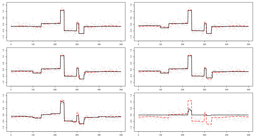
Figure 6. An example of model (41) for $a=0.01$, $b=0.1$ and $\sigma=0.2$. From top left to bottom right: SMUCE, mBIC, unbalhaar, CBS, $\text{FL}^{\text{MSE}}$ and $\text{FL}^{\text{cp}}$ (solid black line) and the true signal (dashed red line).

Again, we note that Table 1 can be complemented by the simulation study in (Zhang and Siegmund, 2007) which accounts for the classical BIC (Schwarz, 1978) and the method suggested in (Fridlyand et al., 2004).

5.2. Gaussian variance regression

Again, we consider normal data $Y_{i}$, however, in contrast to the previous section we aim to estimate the variance $\sigma^{2}\in\mathcal{S}$. For simplicity we set $\mu=0$. This constitutes a natural exponential family with natural parameter $\theta=-(2\sigma^{2})^{-1}$ and $\psi(\theta)=-\log(-2\theta)/2$ for the sufficient statistic $Z_{i}=Y_{i}^{2}$, $i=1,\ldots,n$. It is easily seen that the MR-statistic in this case reads as

$$T_{n}(Z,\hat{\sigma}^{2})=\max_{0\leq k\leq\hat{K}}\max_{\hat{l}_{k}<i\leq j\leq\hat{l}_{k+1}}\left(\frac{\sqrt{j-i+1}}{\sqrt{2}}\sqrt{\frac{\overline{Z}_{i}^{j}}{\hat{\sigma}_{k}^{2}}-\log\frac{\overline{Z}_{i}^{j}}{\hat{\sigma}_{k}^{2}}-1}-\sqrt{2\log\frac{en}{j-i+1}}\right).$$

After selecting the model $\hat{K}(q)$ according to (18), the SMUCE is given by

$$\hat{\sigma}^{2}(q)=\operatorname*{\textnormal{argmax}}_{\hat{\sigma}^{2}\in\mathcal{S}_{n}[\hat{K}(q)]}\sum_{k=0}^{\hat{K}(q)}(\hat{l}_{k+1}-\hat{l}_{k})\left(\log\frac{1}{\hat{\sigma}_{k}^{2}}-\frac{\overline{Z}_{\hat{l}_{l}}^{\hat{l}_{k+1}}}{\hat{\sigma}_{k}^{2}}\right),\quad\text{ s.t. }\quad T_{n}(Z,\hat{\sigma}^{2})\leq q.$$

We compare our method to (Höhenrieder, 2008; Davies et al., 2012). Similar to SMUCE they propose to minimize the number of change-points under a multiscale constraint. They additionally restrict their final estimator to coincide with the local maximum likelihood estimator on constant segments. As pointed out by the authors this may increase the number of detected change-points. Following their simulation study we consider test signals $\sigma_{k}$ with $k=0,1,4,9,19$ equidistant change-points and constant values alternating from 1 to 2 ($k=1$), from 1 to 2 ($k=4$), from 1 to 2.5 ($k=9$) and from 1 to 3.5 ($k=19$). For this simulation the parameter of both procedures are chosen such that the number of changes should not be overestimated with probability $0.9$. For any signal we computed both estimates in $1000$ simulations. The difference of true and estimated number change-points as well as the MISE and MIAE are shown in Table 2. Considering the number of correctly estimated change-points, it shows that SMUCE performs better for few changes ($k=1,4,9$) and worse for many changes ($k=19$). This may be explained by the fact that the multiscale test in (Davies et al., 2012) does not include a scale-calibration and is hence more sensible on small scales than on larger ones, see also Subsection 6.2. With respect to MISE and MIAE the SMUCE outperforms in every scenario, interestingly even for $k=19$, where (Davies et al., 2012) performs better w.r.t. the estimated number of change-points.

	k	-3	-2	-1	0	+1	+2	+3	MISE	MIAE
SMUCE	0	0.000	0.000	0.000	0.945	0.053	0.002	0.000	0.00072	0.02040
(Davies et al., 2012)	0	0.000	0.000	0.000	0.854	0.127	0.019	0.000	0.00093	0.02122
SMUCE	1	0.000	0.000	0.000	0.975	0.024	0.001	0.000	0.00653	0.04295
(Davies et al., 2012)	1	0.000	0.000	0.000	0.901	0.089	0.009	0.001	0.00935	0.04648
SMUCE	4	0.000	0.000	0.000	0.997	0.003	0.000	0.000	0.02153	0.07967
(Davies et al., 2012)	4	0.000	0.000	0.000	0.957	0.042	0.001	0.000	0.03378	0.09655
SMUCE	9	0.000	0.001	0.023	0.973	0.003	0.000	0.000	0.06456	0.13206
(Davies et al., 2012)	9	0.000	0.000	0.009	0.968	0.023	0.000	0.000	0.11669	0.18297
SMUCE	19	0.000	0.027	0.222	0.751	0.000	0.000	0.000	0.26076	0.27468
(Davies et al., 2012)	19	0.000	0.008	0.074	0.912	0.006	0.000	0.000	0.47105	0.40606

Table 2. Comparison of SMUCE and the method in (Davies et al., 2012). Difference between the estimated and the true number of change-points for $k=0,1,4,19$ change-points as well as MISE and MIAE for both estimators.

5.3. Poisson regression

We consider the Poisson-family of distributions with intensity $\mu>0$. Then, $\theta=\log\mu$ and $\psi(\theta)=\exp\theta$. The MR-statistic is computed as

$$T_{n}(Y,\hat{\mu})=\max_{0\leq k\leq\hat{K}}\max_{\hat{l}_{k}<i\leq j\leq\hat{l}_{k+1}}\left(\sqrt{2(j-i+1)}\sqrt{\overline{Y}_{i}^{j}\log\frac{\overline{Y}_{i}^{j}}{\mu_{k}}+\mu_{k}-\overline{Y}_{i}^{j}}-\sqrt{2\log\frac{en}{j-i+1}}\right).$$

For $\hat{K}(q)$ as in (18), the SMUCE is given by

$$\hat{\mu}(q)=\operatorname*{\textnormal{argmax}}_{\hat{\mu}\in\mathcal{S}_{n}[\hat{K}(q)]}\sum_{k=0}^{\hat{K}(q)}(\hat{l}_{k+1}-\hat{l}_{k})(\overline{Y}_{\hat{l}_{l}}^{\hat{l}_{k+1}}\log\hat{\mu}_{k}-\hat{\mu}_{k})\quad\text{ s.t. }\quad T_{n}(Y,\hat{\mu})\leq q.$$

In applications (c.f. the example from photoemission spectroscopy below), one is often faced with the problem of low count Poisson data, i.e. when the intensity $\mu$ is small. It will turn out that in this case, data transformation towards Gaussian variables such as variance stabilizing transformations are not always sufficient and it pays off to take into account the Poisson likelihood into SMUCE.

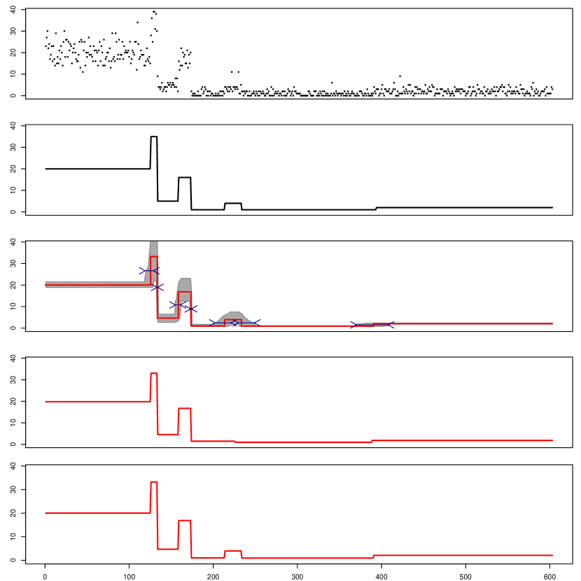
Figure 7. from top to bottom: simulated data, true signal, SMUCE with confidence bands for the signal intensities (gray area) and confidence intervals for the change-points (inward pointed arrows), $\text{SMUCE}_{\text{mm}}$ and Ploracle.

In the following we perform a simulation study where we use a signal with a low count and a spike part (see top panel of Figure 7). In order to evaluate the performance of the SMUCE we compare it to the BIC estimator and the PLoracle as described before. Moreover, we included a version of the SMUCE which is based on variance stabilizing transformations of the data. To this end, we applied the mean-matching transformation (Brown et al., 2010) to preprocess the data. We then compute the SMUCE under a Gaussian model and retransform the obtained estimator by the inverse mean-matching transform. The resulting estimator is referred to as $\text{SMUCE}_{\text{mm}}$. Moreover, as a benchmark, we compute the (parametric) maximum likelihood estimator with $K=7$ change-points, which is referred to as MLoracle.

	$\leq$5	6	7	8	$\geq$9	MISE	MIAE	Kullback-Leibler
SMUCE	0.000	0.067	0.929	0.004	0.004	0.274	0.217	0.0187
$\text{SMUCE}_{\text{MS}}$	0.000	0.067	0.929	0.004	0.004	0.282	0.219	0.0194
BIC	0.000	0.000	0.080	0.094	0.920	0.575	0.313	0.0417
$\text{SMUCE}_{\text{mm}}$	0.013	0.420	0.561	0.005	0.006	0.434	0.364	0.0418
PLoracle	0.045	0.014	0.942	0.000	0.000	0.275	0.217	0.0185
MLoracle	0.000	0.000	1.000	0.000	0.000	0.258	0.208	0.0143

Table 3. Frequencies of $\hat{K}$ and distance measures for SMUCE, the BIC (Schwarz, 1978), the SMUCE for variance stabilized signals as well as the PLoracle and MLoracle.

Table 3 summarizes the simulation results. As to be expected the standard BIC performs far from satisfactorily. We stress that SMUCE clearly outperforms the $\text{SMUCE}_{\text{mm}}$, which is based on Gaussian transformations. Note, that the $\text{SMUCE}_{\text{mm}}$ systematically underestimates the number of change-points $K=7$ which highlights the difficulty to capture those parts of the signal correctly, where the intensity is low. Again, SMUCE performs almost as good as the Poisson-oracle PLoracle. To get a visual impression along with the results of Table 3, we illustrated these estimators in Figure 7.

5.4. Quantile regression

Finally, we extend our methodology to quantile regression. Let the observations $Y_{1},\ldots,Y_{n}$ be given by model (1), without any assumption on the underlying distribution. For some $\beta\in(0,1)$, we now aim for estimating the corresponding (piecewise-constant) $\beta$-quantile function, which will be denoted by $\vartheta_{\beta}$. This problem can be turned into a Bernoulli regression as follows: Given the $\beta$-quantile function $\vartheta_{\beta}$ define the random variables $W(\vartheta)=(W_{1},\ldots,W_{m})$ as

$$W_{i}=\begin{cases}1&\text{ if }Y_{i}\leq\vartheta_{\beta}(i/n)\\ 0&\text{ otherwise }\end{cases},\quad i=1,\ldots,n.$$

Then, $W_{1},\ldots,W_{n}$ are i.i.d. Bernoulli random variables with mean value $\beta$. Extending the idea in Subsection 1.1 we compute a solution of (6), where $T_{n}(W(\vartheta_{\beta}))$ denotes the multiscale statistic for Bernoulli observations which reads as

$$T_{n}(W(\vartheta_{\beta}),\beta)=\max_{\begin{subarray}{c}1\leq i\leq j\leq n\\ \vartheta_{\beta}\text{is constant on }[i/n,j/n]\end{subarray}}\left(\sqrt{2T_{i}^{j}(W(\vartheta_{\beta}),\beta)}-\sqrt{2\log\frac{en}{j-i+1}}\right)$$

with

$$T_{i}^{j}(W(\vartheta_{\beta})),\beta)=(j-i+1)\left(\bar{W}_{i}^{j}\log\left(\frac{\bar{W}_{i}^{j}}{{\beta}}\right)+(1-\bar{W}_{i}^{j})\log\left(\frac{1-\bar{W}_{i}^{j}}{1-{\beta}}\right)\right).$$

In other words, we compute the estimate with fewest change-points, such that the signs of the residuals fulfill the multiscale test for Bernoulli observations with mean $\beta$. The computation of this estimate hence results in the same type of optimization problem as treated in subsection 3.1 and we can apply the proposed methodology.

In the following we compare this approach with a generalized taut string algorithm (Davies and Kovac, 2001), which was proposed in (Dümbgen and Kovac, 2009), for estimating quantile functions. The estimate is constructed in such a way that it minimizes the number of local extreme values among a specified class of functions. Here, a local extreme value is either a local maximum or a local minimum.

In contrast to SMUCE the number of change-points is not penalized. In a simulation study the authors showed that their method is particularly suitable to detect local extremes of a signal. We follow this idea and repeated their simulations. The results which also include the estimated number of change-points, are shown in Table 4. It can be seen that the gen. taut string estimates the number of local extremes slightly better than SMUCE, while the number of change-points is overestimated for $n=2048$ and $n=4096$. This may be explained by the fact that the generalized taut string is not primarily designed to have few change-points rather few local extremes.

		local extreme values			change-points
	n	$\beta=0.5$	$\beta=0.1$	$\beta=0.9$	$\beta=0.5$	$\beta=0.1$	$\beta=0.9$
SMUCE	$512$	3 (5.9)	1 (7.9)	2 (7.4)	5 (5.8)	2 (9.1)	3 (8.3)
gen. taut string	$512$	3(6.0)	3 (6.6)	3 (6.6)	12 (2.0)	6 (4.9)	7 (4.0)
SMUCE	$2048$	9 (0.4)	4 (5.4)	3 (5.8)	11 (0.1)	6 (5.2)	5 (5.9)
gen. taut string	$2048$	9 (0.7)	5 (4.0)	3 (5.7)	26 (15.3)	18 (7.1)	16 (5.7)
SMUCE	$4096$	9 (0.1)	4 (4.3)	5 (4.5)	11 (0.2)	8 (3.1)	6 (4.8)
gen. taut string	$4096$	9 (0.0)	6 (3.1)	3 (5.3)	35 (24.1)	25 (13.8)	21 (9.9)

Table 4. Comparison of SMUCE and generalized taut string (Dümbgen and Kovac, 2009). Median of local extreme values/ change-points of the estimators and mean absolute difference (in brackets) to true number of local extremes/ change-points. The true number of local extremes equals $9$ and the true number of change-points equals $11$.

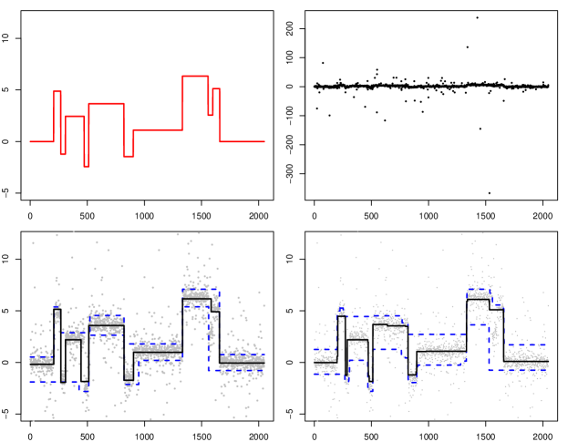
Figure 8. First row: block signal (left) and simulated data (right). Second row: Estimator for median (solid), 0.1 and 0.9-quantiles (dashed) from SMUCE (left) and generalized taut string (right)

5.5. On the coverage of confidence sets $I(q)$

In Section 2.6 we gave asymptotic results on the simultaneous coverage of the confidence sets $I(q)$ as defined in (28). In our simulations we choose $q=q_{1-\alpha}$ to be the $1-\alpha$-quantile of $M$ as in (15). It then follows from Corollary 2.10 that asymptotically the simultaneous coverage is larger than $1-\alpha$. We now investigate empirically the simultaneous coverage of $I(q_{1-\alpha})$. To this end, we consider the test signals shown in Figure 9 for Gaussian observations with varying mean, Gaussian observations with varying variance, Poisson observations and Bernoulli observations.

Table 5 summarizes the empirical coverage for different values for $\alpha$ and $n$ obtained by $500$ simulation runs each and the relative frequencies of correctly estimated change-points, which are given in brackets. The results show that for $n=2000$ the empirical coverage exceeds $1-\alpha$ in all scenarios. The same is not true for smaller $n$ (indicated by bold letters), since here the number of change-points is misspecified rather frequently (see numbers in brackets). Given $K$ has been estimated correctly, we find that the empirical coverage of bands and intervals is in fact larger than the nominal $1-\alpha$ for all simulations.

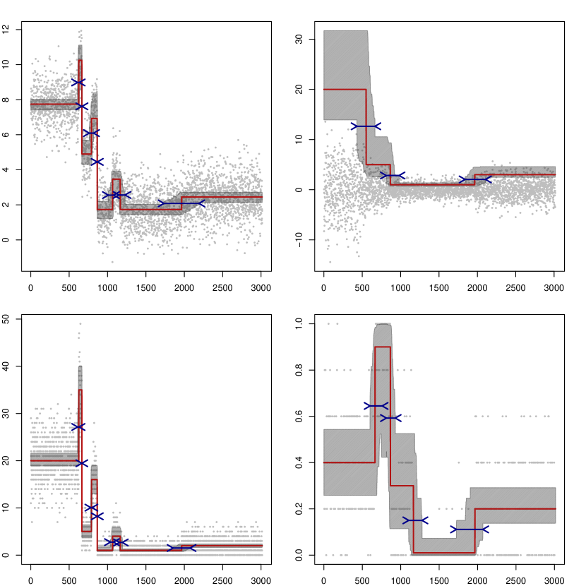
Figure 9. f.l.t.r.: Gaussian observations with varying mean, Gaussian observations with varying variance, Poisson and (binned) Bernoulli observations and SMUCE (solid red line) with confidence bands (grey hatched) and confidence intervals for change-points (inwards pointing arrows).

$n$	$1-\alpha$	Gaussian			Gaussian			Poisson			Bernoulli
		(mean)			(variance)
	$0.8$	0.59	0.64	0.92	0.66	0.68	0.97	0.87	0.89	0.98	0.85	0.90	0.94
$1000$	$0.9$	0.48	0.49	0.98	0.39	0.39	1.00	0.85	0.86	0.99	0.86	0.86	0.99
	$0.95$	0.28	0.28	1.00	0.16	0.18	0.93	0.71	0.74	0.96	0.66	0.70	0.94
	$0.8$	0.84	0.90	0.93	0.87	0.88	0.98	0.92	0.95	0.96	0.93	0.97	0.96
$1500$	$0.9$	0.73	0.74	0.98	0.72	0.74	0.97	0.95	0.97	0.98	0.96	0.97	0.99
	$0.95$	0.55	0.56	0.98	0.45	0.47	0.98	0.92	0.93	0.99	0.89	0.90	0.99
	$0.8$	0.94	0.99	0.95	0.98	1.00	0.98	0.95	0.99	0.95	0.96	0.99	0.97
$2000$	$0.9$	0.98	1.00	0.98	0.99	1.00	0.99	0.96	0.99	0.96	0.97	0.99	0.98
	$0.95$	0.99	1.00	0.99	0.97	0.99	0.98	1.00	1.00	1.00	0.99	1.00	0.99

Table 5. Empirical coverage obtained from $500$ simulations for the signals shown in Figure 9. For each choice of $\alpha$ and $n$ we computed the simultaneous coverage of $I(q)$, as in (28) (first value), the percentage of correctly estimated number of change-points (second value) and the simultaneous coverage of confidence bands and intervals for the change-points given $\hat{K}(q)=K$ (third value).

5.6. Real data results

In this section we analyze two real data examples. The examples show the variety of possible applications for SMUCE. Moreover, we revisit the issue of choosing $q$ as proposed in Section 4 and illustrate its applicability to the present tasks.

5.6.1. Array CGH data

Array Comparative Genomic Hybridization (CGH) data show aberrations in genomic DNA. The observations consist of the log-ratios of normalized intensities from disease and control samples. The statistical problem at hand is to identify regions on which the ratio differs significantly from $0$ (which corresponds to a gain or a loss). These are often referred to as aberration regions.

A thorough overview of the topic and a comparison of several methods is given in (Lai et al., 2005). We compute the SMUCE for two data sets studied in (Lai et al., 2005) and more recently in (Du and Kou, 2012; Tibshirani and Wang, 2008). The data sets show the Array-CGH profile of chromosome 7 in GBM29 and chromosome 13 in GBM31, respectively (see also again (Du and Kou, 2012; Lai et al., 2005)).

By means of these two data examples we illustrate how the developed theory in Section 2 can be used for applications. As it was stressed in (Lai et al., 2005) many algorithms in change-point detection do strongly depend on the proper choice of a tuning parameter, which is often a difficult task in practice. We point out that our proposed choice of the threshold parameter $q$ has in fact a statistical meaningful interpretation as it determines the level of the confidence set $C(q)$. Moreover, we will emphasize the usefulness of confidence bands and intervals for Array CGH data.

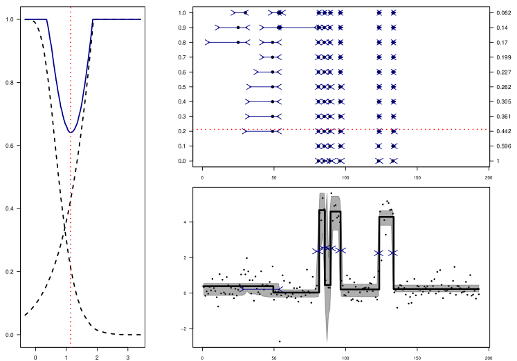
Figure 10. Left: Probability for over/underestimating (decreasing/increasing dashed line) the number of change-points in dependence of $q$ ($x$-axis) and their sum (solid line). Top right: Detected change-points with confidence intervals for different values of $\alpha$ (left $y$-axis) with the probabilty of underestimation (right $y$-axis). Bottom right: SMUCE (solid line) computed for the optimal $q^{*}\approx 1.1$ with confidence bands (grey hatched) and confidence intervals for change-points (inwards pointing arrows).

We first consider the GBM29 data. In order to choose $q$ according to the suggested proceeding in (37), assumptions on $\lambda$ and $\Delta$ have to be imposed. As mentioned above log ratios of copy numbers may take on a finite number of values which are approximately $\left\{\log(1),\log(3/2),\log(2),\log(5/2),\ldots\right\}.$ It therefore seems reasonable to assume that the smallest jumps size is $\Delta=log(3/2)$. Moreover, we choose $\lambda\geq 0.2$.We stress that the final solution of the SMUCE will not be restricted to these assumptions. They enter as prioir assumptions for the choice of $q$. If the data speak strongly against these assumptions SMUCE will adapt to this.

In the left panel of Figure 10 we depict the probability of overestimating the number of change-points as a function of $q$ (decreasing dashed line) and the probability of overestimating the number of change-points as a function of $q$ (increasing dashed line) under the above stated assumption on $\lambda$ and $\Delta$. One may interpret the plot in the following way. It provides a tool for finding jumps of minimal height $\Delta=log(3/2)$ on scales of at least $\lambda=0.2$. For the optimized $q^{*}$ we obtain, that the number jumps is misspecified with probability less than $0.35$. For the corresponding estimate see Figure 10.

Moreover, for different choices of $q$ we displayed the SMUCE. The top-right panel of Figure 10 shows the estimated change-points with its confidence intervals. Bounds for the probability that $K$ is overestimated can be found on the left axis, bounds for underestimation on the right axis.

Note from the top-right image in Figure 10 that the SMUCE is quite robust w.r.t. $q=q_{1-\alpha}$. For $\alpha\in[0.2,0.7]$ SMUCE always detects exactly $7$ change-points in the signal. The results show that a jump of the size $\approx\Delta$ is found in the data on an interval, which length is even slightly smaller than $\lambda$. However, SMUCE is also able to detect larger abberations on smaller intervals, which makes it quite robust against wrong choices of $\Delta$ and $\lambda$.

Recall that one goal in Array CGH data analysis is to determine segments on which the signals differs from $0$. The confidence sets in the right lower plot indicate three intervals with signal different from $0$. Moreover, as indicated by the blue arrows, the change-point locations are detected very precisely. Actually, the estimator suggests one more change-point in the data. However, it can be seen from the confidence bands that there is only small evidence for the signal to be nonzero. Further, the confidence bands may be used to decide which segments belong to the same copy number event. In this particular example the confidence bands suggest that these three segments belong to the same copy number event, i.e. have the same mean value.

Put differently, not only an estimator for the true signal is obtained, but also $3$ regions of abberation were detected and simultaneous confidence intervals for the signal’s value on this regions at a level of $1-\alpha=0.9$ are given. This is in accordance with others’ findings (Lai et al., 2005; Du and Kou, 2012).

captionLeft: Probability for over/underestimating (decreasing/increasing dashed line) the number of change-points in dependence of $q$ ($x$-axis) and their sum (solid line). Top right: Detected change-points with confidence intervals for different values of $\alpha$ (left $y$-axis) with the probabilty of underestimation (right $y$-axis). Bottom right: SMUCE (solid line) computed for the optimal $q^{*}\approx 1.7$ with confidence bands (grey hatched) and confidence intervals for change-points (inwards pointing arrows).

The same procedure as above is repeated for the GBM31 data as shown in Figure 5.6.1. For the bounds on underestimating the number of change-points we assumed again that $\Delta\geq\log(3/2)$ and chose $\lambda\geq 0.025$. The plots in Figure 5.6.1 show that $\Delta\geq\log(3/2)$ for the sample size of $n=797$ the probability of misspecification can be bounded by $\approx 0.12$ for the minimal length $\lambda=0.025$, which corresponds to $19$ observations. Using the same reasoning as above we identify one large region of abberation and obtain a confidence interval for the corresponding change-point as well as for the signal’s value. Here, the optimized $q^{*}\approx 1.7$ in the sense of (38) gives $\alpha\approx 0.04$ which yields a SMUCE with one jump with high significamce.

5.6.2. Photoemission Spectroscopy (PES)

Electron emission from nanostructures triggered by ultrashort laser pulses has numerous applications in time-resolved electron imaging and spectroscopy (Ropers et al., 2007). In addition, it holds promise for fundamental insight into electron correlations in microscopic volumes, including antibunching (Kiesel et al., 2002). Single-shot measurements of the number of electrons emitted per laser pulse (Bormann et al., 2010; Herink et al., 2012) will allow for the disentanglement of various competing processes governing the electron statistics, such as classical fluctuations, Pauli blocking and space charge effects.

Figure 11. Top: Detected change-points and confidence intervals for different values of $\alpha$ ($y$-axis). Middle: SMUCE with confidence bands (grey hatched), confidence intervals for the changepoints (inwards pointing arrows) and binned PES data. Bottom: ML-Estimator with 10 change-points.

We investigate with the SMUCE approach PES data displayed in the bottom panel of Figure 11. It represents a time series of electron numbers recorded from a PES experiment performed in the Ropers lab (Department of Biophysics, University of Goettingen, see (Bormann et al., 2010)). It is custom to model PES data by Poisson regression with unknown intensity. This intensity is known to show long term fluctuations which correspond to variation in laser power and laser beam pointing, which cannot be controlled in the experiment and typically leads to an overall over-dispersion effect. However, on a short time scale, the interesting task is to investigate underdispersion in the distribution. Such underdispersion would indicate an electron interaction in which the emission of one (or a few) electrons decreases the likelihood of further emission events. Specifically, a significant underdispersion in the single-shot electron number histogram would evidence an anticorrelation caused by electrons being Fermions that obey the Pauli exclusion principle. A piecewise constant mean that models sudden changes in the laser intensity to reflect the large scale fluctuations is used for segmentation of the data for further investigation of under- or overdispersion in these segments.

Figure 11 shows the estimated change-points of SMUCE (and the corresponding confidence intervals) for $\alpha=0.05,0.1,\ldots,0.9$ in the top panel. We also display the SMUCE with confidence bands for $\alpha=0.9$ (middle) and for comparison the MLE with $\hat{K}_{\text{SMUCE}}(q)=10$ change-points (bottom). Note, that the MLE is computed without the additional constraint $T_{n}(Y,\hat{\mu})\leq q$, in contrast to SMUCE. Remarkably, this results in a different estimator.

We estimate the dispersion of data $Y_{1},\ldots,Y_{m}$ by $\hat{\rho}=\hat{\sigma}^{2}$/$\hat{\mu}$, where $\hat{\mu}=1/m\sum_{i=1}^{m}Y_{i}$ and $\hat{\sigma}=1/m\sum_{i=1}^{m}(Y_{i}-\hat{\mu})^{2}$. In Table 6 $\hat{\mu}=1/m\sum_{i=1}^{m}Y_{i}$ is shown for the whole dataset as well as for the segments identified by SMUCE. It can be seen that our segmentation allows to explain the overall overdispersion to a large extent, by the long term fluctuations. However, the results in Table 6 do not indicate significant underdispersion on any of the identified segments. This may be explained by a masking effect due to fluctuations of the emission current. Future experiments using more stable emission currents are underway.

segment	overall	1	2	3	4	5	6	7	8	9	10	11
$\hat{\rho}$	1.02	0.98	1.02	0.98	1.04	1.01	1.04	0.98	1.03	0.99	0.98	1.05

Table 6. Dispersion estimator $\hat{\rho}$ of the whole dataset and on the segments identified by SMUCE

6. Discussion

6.1. Dependent Data

So far the theoretical justification for SMUCE relies on the independence of the data in model (1) (see Section 2), as for example the optimal power results in Section 2.5. We claim, however, that SMUCE as introduced in this paper can be extended to piecewise constant regression problems with serially dependent data. A comprehensive discussion is above the scope of this paper an will be addressed in future work. Here, we confine ourselves to the case of a Gaussian moving average process of order 1, a similar strategy has been applied in (Hotz et al., 2012) for $m$-dependent data.

Example 6.1.

For a piecewise constant function $\mu\in\mathcal{S}$ we consider the MA(1) model

$$Y_{i}=\mu(i/n)+\varepsilon_{i}+\beta\varepsilon_{i-1}\quad\text{ for }\quad i=1,\ldots,n,$$

where $\beta<1$ and $\varepsilon_{0},\varepsilon_{1},\ldots,\varepsilon_{n}\overset{i.i.d.}{\sim}\mathcal{N}(0,\sigma^{2})$. We aim to adapt the SMUCE to this situation. Following the local likelihood approach underlying the multiscale constraint in (2) one simply might replace the local statistic $\sqrt{2T_{i}^{j}(Y,\mu_{0})}$ for $\mu_{0}\in\mathbb{R}$ in (3) by the (modified) local statistics

$$\sqrt{2\tilde{T}_{i}^{j}(Y,\mu_{0})}=\frac{\left|\sum_{l=i}^{j}Y_{l}-\mu_{0}\right|}{\sqrt{\sigma^{2}\left[(j-i+1)(1+\beta^{2})+(j-i)\beta\right]}}.$$ (42)

This is motivated by the fact, that $\text{Var}(\sum_{l=i}^{j}Y_{l})=\sigma^{2}\left[(j-i+1)(1+\beta^{2})+(j-i)\beta\right]$. Under the null-hypothesis the local statistics $\tilde{T}_{i}^{j}$ then marginally have a $\chi^{2}_{1}$ distribution, as $T_{i}^{j}$ in (4) for independent Gaussian observations.

In order to control the overestimation error as in Section 2.3, one now has to compute the null distribution of

$$\tilde{T}_{n}(Y,\mu)=\max_{\begin{subarray}{c}1\leq i<j\leq n\\ \mu(t)=\mu_{0}\text{ for }t\in[i/n,j/n]\end{subarray}}\left(\sqrt{2\tilde{T}_{i}^{j}(Y,\mu_{0})}-\sqrt{2\log\frac{en}{j-i+1}}\right).$$

To this end, we used Monte-Carlo simulations for a sample size of $n=500$. We reconsider the test signal from Section 5.1 with $\sigma=0.2$ and $a=0$. The empirical null-distribution of $\tilde{T}_{n}$ and a probability-probability plot of the null distribution of $T_{n}$ against $\tilde{T}_{n}$ are shown in Figure 12.

Figure 12. ecdf of the null distribution for dependent observations with $\beta=0.3$ and PP plot against the null distribution for independent observations.

For $\beta=0.1$ and $\beta=0.3$, which corresponds to a correlation of $\rho=0.1$ and $\rho=0.27$, we ran $1000$ simulations each. We computed the modified SMUCE, as in (42), and the SMUCE for independent Gaussian observations. For both procedures we chose $q$ to be the $0.75$-quantile of the null-distribution. The results are shown in Table 7. For $\beta=0.1$ both procedures perform similarly, which indicates that SMUCE is robust to such weak dependences, while for $\beta=0.3$ the modified version performs much better w.r.t. the estimated number of change-points.

	$\beta$	5	6	7	8	$\geq 9$	MISE	MIAE
modified SMUCE	0.1	0.02	0.98	0.00	0.00	0.00	0.00154	0.02104
SMUCE	0.1	0.00	0.95	0.04	0.00	0.00	0.00142	0.02117
modified SMUCE	0.3	0.27	0.73	0.00	0.00	0.00	0.00435	0.03084
SMUCE	0.3	0.00	0.29	0.34	0.24	0.13	0.00277	0.03229

Table 7. Frequencies of estimated number of change-points and MISE by model selection for the modified SMUCE and SMUCE.

The example illustrates that SMUCE as in (2) can be successfully applied to the case of dependent data after an adjustment of the underlying multiscale statistic $T_{n}$ to the dependence structure. The asymptotic null-distribution of this modified multiscale statistic is certainly not obvious and postponed to future work.

6.2. Scale-calibration of $T_{n}$

The penalization of different scales as in (3) is borrowed from (Dümbgen and Spokoiny, 2001) and calibrates the number of intervals on a given scale. This prevents the small intervals to dominate the statistic. For this purpose, one might also consider the statistic

$$T^{1}_{n}(Y,\vartheta)=\max_{\begin{subarray}{c}1\leq i<j\leq n\\ \vartheta(t)=\theta\text{ for }t\in[i/n,j/n]\end{subarray}}\left(\frac{T_{i}^{j}(Y,\theta)-2\log\frac{n}{j-i+1}}{\log\log\frac{e^{e}n}{j-i+1}}\right),$$

which is finite a.s. as $n\rightarrow\infty$ (see again (Dümbgen and Spokoiny, 2001, Theorem 6.1) or (Schmidt-Hieber et al., 2011)). A multiscale statistic without scale calibration

$$T^{2}_{n}(Y,\vartheta)=\max_{\begin{subarray}{c}1\leq i<j\leq n\\ \vartheta(t)=\theta\text{ for }t\in[i/n,j/n]\end{subarray}}T_{i}^{j}(Y,\theta).$$

was e.g. considered in (Davies et al., 2012). We illustrate the calibration effect of the statistics $T_{n}$, as in (3), $T_{n}^{1}$ and $T_{n}^{2}$ in Figure 13. The graphic shows the frequencies at which the corresponding $0.75$-quantiles of the statistics $T_{n}$, $T_{n}^{1}$ and $T_{n}^{2}$ is exceeded at a certain scale (scales are displayed on the $x$-axis). It can be seen, that $T_{n}^{2}$ puts much emphasis on small scales, while the penalized statistics $T_{n}$ and $T_{n}^{1}$ distribute the scales more uniformly. For our purposes this calibration is beneficial in two ways: First it is required to obtain the optimal detection rates in Theorem 2.7 and Theorem 2.7 as it was shown in (Chan and Walther, 2013). Second, the asymptotical behavior is determined by a process of the type (16) and not by a extreme value limit as to be expected in the uncalibrated case, where the maximum is attained at scales of the magnitude $\log n$ with high probability (see (Kabluchko and Munk, 2009, Theorem 3.1 and the proof of Theorem 1.1)) in accordance with Figure 13.

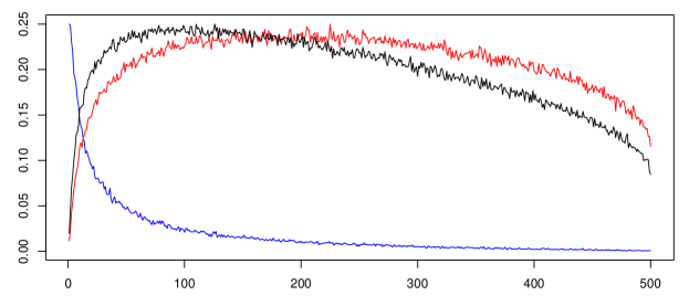
Figure 13. Frequencies of violations of the multiscale constraint for the different multiscale statistics $T_{n}$ (black), $T_{n}^{1}$ (red) and $T_{n}^{2}$ (blue) obtained from 10.000 simulations on certain scales (scales are on the $x$-axis).

6.3. SMUCE from a linear models perspective

For normal mean regression one may rewrite the change-point regression model in (22) as a linear model

$$Y=X\beta+\sigma\epsilon,$$

where $\beta_{i}=\vartheta_{i}-\vartheta_{i-1}$ denotes the jump heights. If we add a vector of ones and a coefficient $\beta_{0}$ to define the offset of the function, then $X$ is an $(n\times n)$ upper triangular matrix with entries $X_{i,j}=1$, $i\geq j$ and zero else. Hence, in the terminology of high dimensional linear models, we have an “$n=p$” problem in contrast to the “$p\gg n$” situation which has perceived enormous attention during the last two decades. If we rescale by $1/\sqrt{n}$, then we find that $X^{t}X/n=\min(i,j)/n$ tends to the covariance function of a standard Brownian motion. From this limiting covariance it becomes immediately clear that assumptions like the restricted isometry property and related conditions (see (Bühlmann and van de Geer, 2011; Candes and Tao, 2007; Meinshausen and Yu, 2009)) fail without additional restrictions, e.g. an $s$-sparseness ($s\ll p$) assumption on the jump locations. For a thorough discussion see (Boysen et al., 2009) or the Appendix in (Harchaoui and Lévy-Leduc, 2010). Roughly speaking, these assumptions guarantee that estimators which are based on minimizing $\ell_{0}(\beta)$, i.e. the number of jumps, can be obtained by the $\ell_{1}(\beta)$ surrogate with large probability. This is not the case in our set up when the number of jumps can be arbitrarily large. This may be taken as a rough explanation for the empirical observations that $TV$ and $\ell_{1}$ penalization method do not perform competitive in the multiscale framework discussed in this paper for estimating location and number of change-points, as they built in too many little jumps. SMUCE employs a weaker notion of sparsity, i.e. $s=n=p$.

6.4. Risk measures

SMUCE aims to maximize the probability of correctly specifying the number of jumps $P(\hat{K}=K)$ uniformly over sequences of models such that $\lambda_{n}\Delta_{n}^{2}$ tends to zero not as fast as $\log n/n$. This is conceptually very different from optimizing $\hat{\vartheta}$ w.r.t. convex risk measures such as the mean squared error and related concepts. The latter measures do not primarily target on the jump locations and number of jumps. Therefore, we argue that in those applications, where the primary focus is on the jump locations SMUCE may be advantageous. In fact, maximizing the probability of correctly estimating the number of jumps as SMUCE advocates has some analogy to risk measures for variable selection problems, shown to perform adequately successful in high dimensional models. This includes the false discovery rate (FDR) (Benjamini and Hochberg, 1995) and related ideas (see e.g. (Genovese and Wasserman, 2004)). Whereas in our context the latter ones aim to minimize the expected relative number of wrongly selected change-points, SMUCE is able to give at the same hand a guarantee that the true change-points will be detected with large probability and hence controls the false acceptance rate (FAR) as well.

6.5. Computational costs

In (Killick et al., 2011) the authors showed that their pruned exact linear time method leads to an algorithm which expected complexity is linear in $n$ in some cases. As stressed in Section 3, our algorithm includes similar pruning steps. Due to the complicated structure of the cost functional, however, it seems impossible to prove such a result for the computation of SMUCE. The computation can, of course, be further reduced significantly if e.g. only intervals of dyadic lengths are incorporated into the multiscale statistic. Since the dynamic approach leads to a recursive computation, SMUCE can be updated in linear time, if applied to sequential data. Another interesting strategy to reduce the computational costs could be adapted from (Walther, 2010; Rivera and Walther, 2012) who suggest to restrict the multiscale constraint to a specific system of intervals of size $\mathcal{O}(n)$ which still guarantees optimal detection.

6.6. The choice of $\alpha$

We have offered a strategy to select the threshold $q=q_{\alpha}$ and hence the confidence level $\alpha$ in a sensible way to minimize $\mathbf{P}(\hat{K}\neq K)$, by balancing the probabilities of over- and underestimation of $K$, simultaneously. This is based on the inequalities in Section 4 depending on $\lambda,\Delta$ and $n$. As indicated in Figures 1,10,5.6.1 and 11 this can be used to consider the evolution of SMUCE depending on $\alpha$ as a universal “objective” smoothing parameter. The features (jumps) of each SMUCE given $\alpha$ then may be regarded as “present with certain confidence” similar in spirit to ideas underlying siZer (see (Chaudhuri and Marron, 1999, 2000)). It is striking that in many simulations we found that features (jumps) remain persistent for a large range of levels $\alpha$. Of course, other strategies to balance $\mathbf{P}(\hat{K}(q)>K)$ and $\mathbf{P}(\hat{K}(q)<K)$ are of interest, e.g. if one of these probabilities is considered as less important. For a first screening of jumps, $\mathbf{P}(\hat{K}(q)>K)$ is the less serious error and $\mathbf{P}(\hat{K}(q)<K)$ should be minimized primarily. This can be achieved by optimizing the convex combination $\delta\mathbf{P}(\hat{K}(q)>K)+(1-\delta)\mathbf{P}(\hat{K}(q)<K)$ for a weight $\delta$ close to 1 along the lines described in Section 4.

7. Supplement to “Multiscale change-point inference”

In this supplement we collect the proofs of the main assertions in the paper together with some auxiliary lemmas. We further give more general versions of some results in the paper.

7.1. Large deviation and power estimates

We begin by recalling some large deviation results for exponential families. By $D(\theta||\tilde{\theta})$ we will denote the Kullback-Leibler divergence of $F_{\theta}$ and $F_{\tilde{\theta}}$, i.e.

$$D(\theta||\tilde{\theta})=\int_{\mathbb{R}}f_{\theta}(x)\log\frac{f_{\theta}(x)}{f_{\tilde{\theta}}(x)}\textnormal{\,d}\nu(x)=\psi(\tilde{\theta})-\psi(\theta)-(\tilde{\theta}-\theta)m(\theta).$$ (43)

With the techniques used in [Thm.7.1]Bro86 it is readily seen that for a sequence of independent and $F_{\theta}$-distributed r.v. $Y_{1},\ldots,Y_{n}$ one has that

$$\mathbf{P}\left(\overline{Y}-m(\theta)\geq\eta\right)\leq e^{n(D(\theta||\theta+\varepsilon)-\eta\varepsilon)}$$ (44)

for all $\varepsilon>0$ such that $\theta+\varepsilon\in\Theta$. The following restatement of inequality (44) turns out to be very useful.

Lemma 7.1.

Let $Y=(Y_{1},\ldots,Y_{n})$ be independent random variables such that $Y_{i}\sim F_{\theta}$ and assume that $\delta>0$ is such that $\theta+\delta\in\Theta$. Then,

$$\mathbf{P}(m^{-1}(\overline{Y})\geq\theta+\delta)\leq e^{-nD(\theta+\delta||\theta)}.$$

Proof.

First observe that according to (44)

$$\mathbf{P}(m^{-1}(\overline{Y})\geq\theta+\delta) =\mathbf{P}(\overline{Y}-m(\theta)\geq m(\theta+\delta)-m(\theta))$$

$$\leq\exp(n(D(\theta||\theta+\delta)-(m(\theta+\delta)-m(\theta))\delta)).$$

Now it follows from (43) that

$$D(\theta||\theta+\delta)-(m(\theta+\delta)-m(\theta))\delta =\psi(\theta+\delta)-\psi(\theta)-m(\theta+\delta)\delta$$

$$=-(\psi(\theta)-\psi(\theta+\delta)-(\theta-(\theta+\delta))m(\theta+\delta))$$

$$=-D(\theta+\delta||\theta).$$

∎

From (44) we further derive a basic power estimate for the likelihood ratio statistic (4).

Lemma 7.2.

Let $Y=(Y_{1},\ldots,Y_{n})$ be independent random variables such that $Y_{i}\sim F_{\theta}$ and assume that $\delta\in\mathbb{R}$ is such that $\theta+\delta\in\Theta$. Then,

$$\mathbf{P}\left(T_{1}^{n}(Y,\theta+\delta)\geq q\right)\geq 1-\exp\left(n\inf_{\varepsilon\in[0,\delta]}\left[D(\theta||\theta+\varepsilon)-\frac{\varepsilon}{\delta}D(\theta||\theta+\delta)+\frac{\varepsilon q}{n\delta}\right]\right).$$

Proof.

For

$$J(\overline{Y},\theta) =\phi(\overline{Y})-\left(\overline{Y}\theta-\psi(\theta)\right)$$

we obtain

$$J(\overline{Y},\theta+\delta)=J(\overline{Y},\theta)-\delta\overline{Y}-\psi(\theta)+\psi(\theta+\delta).$$ (45)

Thus, we have

$$\Pi(q,n,\delta) :=\mathbf{P}\bigl{(}T_{1}^{n}(Y,\theta+\delta)\geq q\bigr{)}$$

$$=\mathbf{P}\left(J(\overline{Y},\theta+\delta)\geq\frac{q}{n}\right)$$

$$=\mathbf{P}\left(J(\overline{Y},\theta)-\delta\overline{Y}\geq\frac{q}{n}-\psi(\theta+\delta)+\psi(\theta)\right)$$

$$\geq\mathbf{P}\left(-\delta\overline{Y}\geq\frac{q}{n}-\psi(\theta+\delta)+\psi(\theta)\right),$$

where in the last inequality holds since $J(x,\theta)\geq 0$ for all $x\in\mathbb{R}$ and $\theta\in\Theta$. Now, let us first assume that $\delta>0$. Then by (43) we find

$$\mathbf{P}\left(-\delta\overline{Y}\geq\frac{q}{n}-\psi(\theta+\delta)+\psi(\theta)\right) =\mathbf{P}\left(\overline{Y}-m(\theta)\leq-\frac{q}{\delta n}+\frac{D(\theta||\theta+\delta)}{\delta}\right).$$ (46)

Combining this with the large deviation inequality (44) yields

$$\Pi(q,n,\delta) \geq 1-\exp\left(n(D(\theta||\theta+\varepsilon)-{\varepsilon\over\delta}D(\theta||\theta+\delta))+{\varepsilon q\over\delta}\right),$$

for all $0\leq\varepsilon\leq\delta$. The case when $\delta<0$ follows analogously. ∎

For Gaussian observations the estimate can be made explicit.

Lemma 7.3.

Let $Y_{1},\ldots,Y_{n}$ be i.i.d. random variables such that $Y_{1}\sim\mathcal{N}(0,1)$ and let $x_{+}=\max(0,x)$ for $x\in\mathbb{R}$. Then,

$$\mathbf{P}\left(T_{1}^{n}(Y,\delta)\geq q\right)\geq 1-\exp\left(-\frac{1}{8}\left(\sqrt{n}\delta-\sqrt{2q}\right)_{+}^{2}\right).$$ (47)

Proof.

Since $D(\theta||\theta+\varepsilon)=\varepsilon^{2}/2$ we find that

$$\inf_{\varepsilon\in[0,\delta]}n\left[D(\theta||\theta+\varepsilon)-\frac{\varepsilon}{\delta}D(\theta||\theta+\delta)+\frac{\varepsilon q}{n\delta}\right]=-\frac{1}{2}\left(\frac{\delta\sqrt{n}}{2}-\frac{q}{\delta\sqrt{n}}\right)^{2}\leq-\frac{1}{8}\left(\sqrt{n}\delta-\sqrt{2q}\right)^{2},$$

if $\sqrt{n}\delta\geq\sqrt{2q}$. ∎

7.2. Proof of Theorem 2.1

Throughout this section we will assume that $Y=(Y_{1},\ldots,Y_{n})$ are independent and identically distributed random variables with $Y_{1}\sim F_{\theta}$ and $\theta\in\Theta$. Without loss of generality we will assume that $m(\theta)=\dot{\psi}(\theta)=0$ and $v(\theta)=\ddot{\psi}(\theta)=1$. Moreover, assume that $(c_{n})_{n\in\mathbb{N}}$ satisfies (13) and introduce $\mathcal{I}(c_{n})=\{(i,j):j-i+1\geq c_{n}n\}$. We start with some approximation results for the extreme value statistic of the partial sums $\overline{Y}_{i}^{j}$.

Lemma 7.4.

There exist i.i.d standard normally distributed r.v. $Z_{1},\ldots,Z_{n}$ on the same probability space as $Y_{1},\dots,Y_{n}$ such that

$$\lim_{n\rightarrow\infty}\sqrt{\log n}\max_{(i,j)\in\mathcal{I}(c_{n})}\left(\sqrt{j-i+1}\left|\bigl{|}\overline{Y}_{i}^{j}\bigr{|}-\bigl{|}\overline{Z}_{i}^{j}\bigr{|}\right|\right)=0\quad\text{a.s.}$$

Proof.

We define the partial sums $S_{0}^{Y}=0$ and $S_{l}^{Y}=Y_{1}+\ldots+Y_{l}$ and observe that $(j-i+1)\bigl{|}\overline{Y}_{i}^{j}\bigr{|}=\left|S_{j}^{Y}-S_{i-1}^{Y}\right|$. Analogously we define $S_{l}^{Z}$. Now let $(i,j)$ such that $j-i+1\geq nc_{n}$ and observe that

$$\left|\frac{\left|S^{Y}_{j}-S^{Y}_{i-1}\right|}{\sqrt{j-i+1}}-\frac{\left|S^{Z}_{j}-S^{Z}_{i-1}\right|}{\sqrt{j-i+1}}\right|\leq\frac{\left|S^{Y}_{j}-S^{Z}_{j}\right|}{\sqrt{nc_{n}}}+\frac{\left|S^{Y}_{i}-S^{Z}_{i}\right|}{\sqrt{nc_{n}}}\leq 2\max_{0\leq l\leq n}\frac{\left|S^{Y}_{l}-S^{Z}_{l}\right|}{\sqrt{nc_{n}}}.$$

It follows from the KMT inequality [Thm. 1]KomMajTus76 and (13) that

$$\sqrt{\log n}\max_{0\leq l\leq n}\frac{\left|S^{Y}_{l}-S^{Z}_{l}\right|}{\sqrt{nc_{n}}}=\textnormal{o}(1)\quad\text{a.s.}$$

∎

Lemma 7.5.

$$\max_{(i,j)\in\mathcal{I}(c_{n})}\left|\sqrt{2T_{i}^{j}(Y,\theta)}-\sqrt{j-i+1}\bigl{|}\overline{Y}_{i}^{j}\bigr{|}\right|=\textnormal{o}_{\mathbf{P}}(1)$$

Proof.

Set $\xi=m^{-1}$ and note that $\xi$ is strictly increasing. Since $\Theta$ is open, there exists for each given $\delta^{\prime}>0$ a $\delta>0$ such that $\xi(B_{\delta}(0))\subset B_{\delta^{\prime}}(\theta)\subset\Theta$. Next define the random variable

$$L_{n}=\max_{1\leq i<j\leq n}\left|\overline{Y}_{i}^{j}\right|\sqrt{j-i+1}.$$

Then it follows from Shao’s Theorem Sha95 that $L_{n}/\sqrt{\log n}$ converges a.s. to some finite constant and we hence find that

$$\max_{(i,j)\in\mathcal{I}(c_{n})}\left|\overline{Y}_{i}^{j}\right|\leq\sqrt{\frac{\log n}{nc_{n}}}\frac{L_{n}}{\sqrt{\log n}}\rightarrow 0\quad\text{ a.s.}$$

Thus, for each $\varepsilon>0$ there exists an index $n_{0}=n_{0}(\varepsilon)\in\mathbb{N}$ such that for all $n\geq n_{0}$

$$\mathbf{P}\left(\max_{(i,j)\in\begin{subarray}{c}\mathcal{I}(c_{n})\end{subarray}}\left|\overline{Y}_{i}^{j}\right|\geq\delta\right)\leq\varepsilon.$$

In other words, $\xi(\overline{Y}_{i}^{j})\in B_{\delta}(\theta)$ uniformly over $\mathcal{I}(c_{n})$ with probability not less than $1-\varepsilon$. Consequently, $\phi(\overline{Y}_{i}^{j})=\max_{\theta\in\Theta}\theta\overline{Y}_{i}^{j}-\psi(\theta)=\xi(\overline{Y}_{i}^{j})\overline{Y}_{i}^{j}-\psi(\xi(\overline{Y}_{i}^{j}))$ which in turn implies that

$$J(\overline{Y}_{i}^{j},\theta)=\phi(\overline{Y}_{i}^{j})-\theta\overline{Y}_{i}^{j}+\psi(\theta)=(\xi(\overline{Y}_{i}^{j})-\theta)\overline{Y}_{i}^{j}-(\psi(\xi(\overline{Y}_{i}^{j}))-\psi(\theta)).$$

Taylor expansion of $\psi$ around $\theta$ gives (recall that $\dot{\psi}(\theta)=0$ and $\ddot{\psi}(\theta)=1$)

$$\psi(\xi(\overline{Y}_{i}^{j}))-\psi(\theta)=\frac{1}{2}(\xi(\overline{Y}_{i}^{j})-\theta)^{2}+\frac{1}{6}\dddot{\psi}(\tilde{\theta})(\xi(\overline{Y}_{i}^{j})-\theta)^{3}$$

for some $\tilde{\theta}\in B_{\varepsilon}(\theta)$. This implies

$$J(\overline{Y}_{i}^{j},\theta)=(\xi(\overline{Y}_{i}^{j})-\theta)(\overline{Y}_{i}^{j})-\frac{1}{2}(\xi(\overline{Y}_{i}^{j})-\theta)^{2}-\frac{1}{6}\dddot{\psi}(\tilde{\theta})(\xi(\overline{Y}_{i}^{j})-\theta)^{3}.$$

Again, Taylor expansion of $\xi=m^{-1}$ around $0$ shows

$$\xi(\overline{Y}_{i}^{j})-\theta=\overline{Y}_{i}^{j}-\frac{\dddot{\psi}(\tilde{\theta})}{2(v(\tilde{\theta}))^{2}}(\overline{Y}_{i}^{j})^{2}$$

for some $\tilde{\theta}\in B_{\delta^{\prime}}(\theta)$. This finally proves that

$$2T_{i}^{j}(Y,\theta)=(j-i+1)J(\overline{Y}_{i}^{j},\theta)=(j-i+1)(\overline{Y}_{i}^{j})^{2}+(j-i+1)f_{n}(\overline{Y}_{i}^{j})$$

where $f_{n}$ is such that $\bigl{|}f_{n}(\overline{Y}_{i}^{j})\bigr{|}\leq C^{2}\cdot(\overline{Y}_{i}^{j})^{3}$ for a constant $C=C(\delta^{\prime})>0$ (independent of $\varepsilon$, $i$ and $j$) and for all $n\geq n_{0}$. It thus holds with probability not less than $1-\varepsilon$ that

$$\max_{(i,j)\in\mathcal{I}(c_{n})}\left|\sqrt{2T_{i}^{j}(Y,\theta^{*})}-\sqrt{j-i+1}\bigl{|}\overline{Y}_{i}^{j}\bigr{|}\right|\leq C\max_{(i,j)\in\mathcal{I}(c_{n})}\left|(j-i+1)\left(\overline{Y}_{i}^{j}\right)^{3}\right|^{1/2}$$

$$= C\max_{(i,j)\in\mathcal{I}(c_{n})}\left|\frac{\sum_{l=i}^{j}Y_{l}}{\sqrt{j-i+1}}(j-i+1)^{-1/6}\right|^{3/2}$$

$$\leq C\left(\frac{L_{n}}{\sqrt{\log n}}\right)^{3/2}\sqrt[4]{\frac{\log^{3}n}{{nc_{n}}}}.$$

From Shao’s Theorem it follows that the last term vanishes almost surely as $n\rightarrow\infty$. ∎

Combination of Lemma 7.4 and 7.5 yields

Proposition 7.6.

There exist i.i.d standard normally distributed r.v. $Z_{1},\ldots,Z_{n}$ on the same probability space as $Y_{1},\dots,Y_{n}$ such that

$$\max_{(i,j)\in\mathcal{I}(c_{n})}\left|\sqrt{2T_{i}^{j}(Y,\theta)}-\sqrt{j-i+1}\bigl{|}\bar{Z}_{i}^{j}\bigr{|}\right|=\textnormal{o}_{\mathbf{P}}(1).$$

Lemma 7.7.

For $n\in\mathbb{N}$, define the continuous functionals $h,h_{n}:\mathcal{C}([0,1])\rightarrow\mathbb{R}$ by

$$h(x,c) = \sup_{\begin{subarray}{c}0\leq s<t\leq 1\\ t-s\geq c\end{subarray}}\left(\frac{\left|x(t)-x(s)\right|}{\sqrt{t-s}}-\sqrt{2\log\frac{e}{t-s}}\right)\quad\text{ and }$$

$$h_{n}(x,c) = \max_{\begin{subarray}{c}1\leq i<j\leq n\\ (j-i+1)/n\geq c\end{subarray}}\left(\frac{\left|x(j/n)-x(i/n)\right|}{\sqrt{(j-i+1)/n}}-\sqrt{2{\log}\frac{en}{j-i+1}}\right),$$

respectively. Moreover assume that $\left\{x_{n}\right\}_{n\in\mathbb{N}}\subset\mathcal{C}([0,1])$ is such that $x_{n}\rightarrow x$ for some $x\in\mathcal{C}([0,1])$. Then $h_{n}(x_{n},c)\rightarrow h(x,c)$.

Proof.

Let $\delta>0$. Then there exists an index $n_{0}\in\mathbb{N}$ such that $\left|x_{n}(t)-x(t)\right|\leq\delta$ for all $n\geq n_{0}$ and $t\in[0,1]$. Thus, it follows directly from the definition that $h_{n}(x)=h_{n}(x_{n})+\mathcal{O}(\delta)$ for $n\geq n_{0}$. Since $u\mapsto\sqrt{2\log e/u}$ is uniformly continuous on $[c,1]$ we consequently have that $h_{n}(x)\rightarrow h(x)$ as $n\rightarrow\infty$ and the assertion follows. ∎

Before we proceed, recall the definition of $M$ in (15). Moreover, we introduce for $0<c\leq 1$ the statistic

$$M(c):=\sup_{\begin{subarray}{c}0\leq s<t\leq 1\\ t-s>c\end{subarray}}\left(\frac{\left|B(t)-B(s)\right|}{\sqrt{t-s}}-\sqrt{2\log\frac{e}{t-s}}\right).$$ (48)

From [Thm. 6.1]DueSpok01supp (and the subsequent Remark 1) it can be seen that $M(c)$ converges weakly to $M$ as $c\rightarrow 0^{+}$.

Proposition 7.8.

Let $c>0$ and define

$$T_{n}^{c}(Y,\theta)=\max_{(i,j)\in\mathcal{I}(c)}\left(\sqrt{2T_{i}^{j}(Y,\theta)}-\sqrt{2\log\frac{en}{j-i+1}}\right).$$

Then $\lim_{c\rightarrow 0^{+}}\lim_{n\rightarrow\infty}T_{n}^{c}(Y,\theta)=M$, weakly.

Proof.

Set $S_{0}=0$ and $S_{n}=Y_{1}+\ldots+Y_{n}$ and let $\left\{X_{n}(t)\right\}_{t\geq 0}$ be the process that is linear on the intervals $[i/n,(i+1)/n]$ with values $X_{n}(i/n)=S_{i}/\sqrt{n}$. We obtain from Donsker’s Theorem that $X_{n}\stackrel{{\scriptstyle\mathcal{D}}}{{\rightarrow}}B$. Now, recall the definition of $h$ and $h_{n}$ in Lemma 7.7 and observe that

$$h_{n}(X_{n},c)=\max_{(i,j)\in\mathcal{I}(c)}\left(\sqrt{j-i+1}\bigl{|}\overline{Y}_{i}^{j}\bigr{|}-\sqrt{2\log\frac{en}{j-i+1}}\right).$$

It hence follows from Lemma 7.5 that

$$\left|T_{n}^{c}(Y,\theta)-h_{n}(X_{n},c)\right|\leq\max_{(i,j)\in\mathcal{I}(c)}\left|\sqrt{2T_{i}^{j}(Y,\theta)}-\sqrt{j-i+1}\bigl{|}\overline{Y}_{i}^{j}\bigr{|}\right|=\textnormal{o}_{\mathbf{P}}(1).$$ (49)

Since $X_{n}\stackrel{{\scriptstyle\mathcal{D}}}{{\rightarrow}}B$, Lemma 7.7 and [Thm. 5.5]Bil68 imply that $h_{n}(X_{n},c)\stackrel{{\scriptstyle\mathcal{D},}}{{\rightarrow}}h(B,c)$. Theorem 4.1 in (Billingsley, 1968) and (49) thus imply that $T_{n}^{c}(Y,\theta)\stackrel{{\scriptstyle\mathcal{D}}}{{\rightarrow}}h(B,c)=M(c)$ as $n\rightarrow\infty$ for all $c>0$. Thus, the assertion finally follows, since $M(c)\rightarrow M$ weakly as $c\rightarrow 0^{+}$ ∎

Theorem 7.9.

Let $Y=(Y_{1},\ldots,Y_{n})$ be independent and identically distributed random variables with distribution $F_{\theta}$, $\theta\in\Theta$. Moreover, assume that $\left\{c_{n}\right\}_{n\in\mathbb{N}}$ is a sequence of positive numbers such that $n^{-1}\log^{3}n/c_{n}\rightarrow 0$ and set

$$T_{n}(Y,\theta,c_{n})=\max_{(i,j)\in\mathcal{I}(c_{n})}\left(\sqrt{2T_{i}^{j}(Y,\theta)}-\sqrt{2\log\frac{en}{j-i+1}}\right).$$

Then, $T_{n}(Y,\theta,c_{n})\rightarrow M$ weakly as $n\rightarrow\infty$.

Proof.

First observe that according to Proposition 7.6 we have for all $t>0$ that

$$\begin{split}\mathbf{P}\left(T_{n}(Y,\theta;c_{n})\leq t\right)&=\mathbf{P}\left(\max_{(i,j)\in\mathcal{I}(c_{n})}\left(\sqrt{j-i+1}\bigl{|}\overline{Z}_{i}^{j}\bigr{|}-\sqrt{2\log\frac{en}{j-i+1}}\right)\leq t\right)+\textnormal{o}(1)\\ &\geq\mathbf{P}\left(\sup_{0\leq s<t\leq 1}\left(\frac{\left|B(t)-B(s)\right|}{\sqrt{t-s}}-\sqrt{2\log\frac{e}{t-s}}\right)\leq t\right)+\textnormal{o}(1)\end{split}$$

This shows that for all $t>0$

$$\liminf_{n\rightarrow\infty}\mathbf{P}(T_{n}(Y,\theta,c_{n})\leq t)\geq\mathbf{P}(M\leq t)$$

Now let $c>0$ be fixed and assume w.l.o.g. $c_{n}<c$ for all $n\in\mathbb{N}$. With $T_{n}^{c}$ as defined in Proposition 7.8 we conversely find

$$\limsup_{n\rightarrow\infty}\mathbf{P}(T_{n}(Y,\theta,c_{n})\leq t)\leq\limsup_{n\rightarrow\infty}\mathbf{P}(T_{n}^{c}(Y,\theta,c_{n})\leq t)=\mathbf{P}(M(c)\leq t).$$

Hence the assertion follows from Proposition 7.8 after letting $c\rightarrow 0^{+}$ and the fact that $M>0$ a.s. ∎

Proof of Theorem 2.1.

Let $T_{n}(Y,\vartheta;c_{n})$ be defined as in (14). From Theorem 7.9 it then follows that

$$T_{n}(Y,\vartheta;c_{n})\stackrel{{\scriptstyle\mathcal{D}}}{{\rightarrow}}\max_{0\leq k\leq K}\sup_{\tau_{k}\leq s<t\leq\tau_{k+1}}\left(\frac{\left|B(t)-B(s)\right|}{\sqrt{t-s}}-\sqrt{2\log\frac{e}{t-s}}\right).$$

Clearly the limiting statistic on the right hand side is stochastically bounded from above by $M$. Conversely, we observe by the scaling property of the Brownian motion that

$$\sup_{\tau_{k}\leq s<t\leq\tau_{k+1}}\left(\frac{\left|B(t)-B(s)\right|}{\sqrt{t-s}}-\sqrt{2\log\frac{e}{t-s}}\right)\\ \stackrel{{\scriptstyle\mathcal{D}}}{{=}}\sup_{0\leq s<t\leq 1}\left(\frac{\left|B(t)-B(s)\right|}{\sqrt{t-s}}-\sqrt{2\log\frac{e}{t-s}+2\log\frac{1}{\tau_{k+1}-\tau_{k}}}\right)\stackrel{{\scriptstyle\mathcal{D}}}{{\geq}}M-\sqrt{2\log\frac{1}{\tau_{k+1}-\tau_{k}}}.$$

∎

7.3. A general exponential inequality

In this section we give a general exponential inequality for the probability that SMUCE underestimates the number of change-points. To this end, we will make use of the functions

$$\kappa_{1}^{\pm}(v,w,x,y) =\inf_{\begin{subarray}{c}v\leq\theta\leq w\\ \theta\pm x\in[v,w]\end{subarray}}\sup_{\varepsilon\in[0,x]}\left[\frac{\varepsilon}{x}\left(D(\theta||\theta\pm x)-y\right)-D(\theta||\theta\pm\varepsilon)\right],$$ (50)

$$\kappa_{2}^{\pm}(v,w,x) =\inf_{\begin{subarray}{c}v\leq\theta\leq w\\ \theta\pm x\in[v,w]\end{subarray}}D(\theta\pm x||\theta).$$ (51)

Theorem 7.10.

Let $q\in\mathbb{R}$ and $\hat{K}(q)$ be defined as in (18). Moreover, assume that $\kappa_{1}^{\pm}$ and $\kappa_{2}^{\pm}$ are defined as in (50) and (51), respectively and set

$$\kappa_{1} =\min\left\{\kappa_{1}^{+}\left(\underline{\theta},\overline{\theta},\frac{\Delta}{2},\frac{\left(q+\sqrt{2\log\frac{2e}{\lambda}}\right)^{2}}{n\lambda}\right),\kappa_{1}^{-}\left(\underline{\theta},\overline{\theta},\frac{\Delta}{2},\frac{\left(q+\sqrt{2\log\frac{2e}{\lambda}}\right)^{2}}{n\lambda}\right)\right\}\;\text{ and }$$

$$\kappa_{2} =\min\left\{\kappa_{2}^{+}\left(\underline{\theta},\overline{\theta},\frac{\Delta}{2}\right),\kappa_{2}^{-}\left(\underline{\theta},\overline{\theta},\frac{\Delta}{2}\right)\right\}.$$

If $\lambda\geq 2c_{n}$, then

$$\mathbf{P}\left(\hat{K}(q)<K\right)\leq 2K\left[e^{-\frac{n\lambda\kappa_{1}}{2}}+e^{-\frac{n\lambda\kappa_{2}}{2}}\right].$$ (52)

Proof.

Let $\Delta$ and $\lambda$ be the smallest jump size and the smallest interval length of the true regression function $\vartheta$, i.e.

$$\Delta=\inf_{1\leq k\leq K}\left|\theta_{k}-\theta_{k-1}\right|\quad\text{ and }\quad\lambda=\inf_{0\leq k\leq K}\tau_{k+1}-\tau_{k}.$$

Now define $K$ disjoint intervals $I_{i}=\left(\tau_{i}-\lambda/2,\tau_{i}+\lambda/2\right)\subset[0,1]$. Let $\theta_{i}^{+}=\max\left\{\theta_{i-1},\theta_{i}\right\}$, $\theta_{i}^{-}=\min\left\{\theta_{i-1},\theta_{i}\right\}$ and split each interval $I_{i}$ accordingly, i.e. $I_{i}^{+}=\{t\in I_{i}:\vartheta(t)=\theta_{i}^{+}\}$ and $I_{i}^{-}=\{t\in I_{i}:\vartheta(t)=\theta_{i}^{-}\}$. Clearly $I_{i}=I_{i}^{-}\cup I_{i}^{+}$.

From the definition of the estimator $\hat{K}(q)$ it is clear that

$$\hat{K}(q)<K\quad\Leftrightarrow\quad\exists\hat{\vartheta}\in\mathcal{S}_{n}[K-1]\text{ such that }T_{n}(Y,\hat{\vartheta})\leq q.$$

If $\hat{\vartheta}\in\mathcal{S}_{n}[K-1]$, then there exists an index $k\in\left\{1,\ldots,K\right\}$ such that $\hat{\vartheta}$ is constant on $I_{k}$. Let $\Omega_{k}=\left\{\exists\hat{\theta}\in\Theta:\sqrt{T_{I_{k}^{+}}(Y,\hat{\theta})}-\sqrt{\log\frac{en}{\#I_{k}^{+}}}\leq\frac{q}{\sqrt{2}}\text{ and }\sqrt{T_{I_{k}^{-}}(Y,\hat{\theta})}-\sqrt{\log\frac{en}{\#I_{k}^{-}}}\leq\frac{q}{\sqrt{2}}\right\}$ Since the $K$ intervals $I_{i}$ are disjoint we find

$$\mathbf{P}(\hat{K}(q)<K) \leq\sum_{k=1}^{K}\mathbf{P}\left(\Omega_{k}\right).$$

If $\hat{\vartheta}\in\mathcal{S}_{n}[K-1]$ is constant on some $I_{k}$ with value $\hat{\theta}$, then either $\hat{\theta}\leq\theta_{k}^{+}-\Delta/2$ or $\hat{\theta}\geq\theta_{k}^{-}+\Delta/2$, by construction. Set

$$\Omega_{k}^{+} =\left\{\exists\hat{\theta}\leq\theta_{k}^{+}-\Delta/2:\sqrt{T_{I_{k}^{+}}(Y,\hat{\theta})}-\sqrt{\log\frac{en}{\#I_{k}^{+}}}\leq\frac{q}{\sqrt{2}}\right\}\$$

$$\Omega_{k}^{-} =\left\{\exists\hat{\theta}\geq\theta_{k}^{-}+\Delta/2:\sqrt{T_{I_{k}^{-}}(Y,\hat{\theta})}-\sqrt{\log\frac{en}{\#I_{k}^{-}}}\leq\frac{q}{\sqrt{2}}\right\}$$

and observe that $\mathbf{P}(\Omega_{k})\leq\mathbf{P}(\Omega_{k}^{+})+\mathbf{P}(\Omega_{k}^{-})$. We proof an upper bound for $\mathbf{P}(\Omega_{k}^{-})$, the same bound can be obtained for $\mathbf{P}(\Omega_{k}^{+})$ analogously. Recall that $\theta\mapsto T_{I_{k}^{-}}(Y,\cdot)$ is convex and has its minimum at $m^{-1}(\overline{Y}_{{I_{k}^{-}}})$. Thus, $T_{I_{k}^{-}}(Y,\hat{\theta})\geq T_{I_{k}^{-}}(Y,\theta^{-}_{k}+\Delta/2)$ whenever $m^{-1}(\overline{Y}_{{I_{k}^{-}}})\leq\theta^{-}_{k}+\Delta/2$. This yields

$$\mathbf{P}\left(\Omega_{k}^{-}\right) \leq\mathbf{P}\left(\Omega_{k}^{-}\cap\left\{m^{-1}(\overline{Y}_{I_{k}^{-}})\leq\theta_{k}^{-}+{\Delta\over 2}\right\}\right)+\mathbf{P}\left(m^{-1}(\overline{Y}_{I_{k}^{-}})>\theta_{k}^{-}+{\Delta\over 2}\right)$$

$$\leq 1-\mathbf{P}\left(T_{I_{k}^{-}}\left(Y,\theta_{k}^{-}+{\Delta\over 2}\right)\geq 1/2\left(q+\sqrt{2\log(2e/\lambda)}\right)^{2}\right)+\mathbf{P}\left(m^{-1}(\overline{Y}_{I_{k}^{-}})>\theta_{k}^{-}+{\Delta\over 2}\right)$$

$$\leq\exp\left(\frac{\lambda n}{2}\inf_{\varepsilon\in[0,\Delta/2]}\left(D(\theta_{k}^{-}||\theta_{k}^{-}+\varepsilon)-\frac{\varepsilon}{\Delta/2}D(\theta_{k}^{-}||\theta_{k}^{-}+\Delta/2)+\frac{2\varepsilon\left(q+\sqrt{2\log(2e/\lambda)}\right)^{2}}{\Delta\lambda n}\right)\right)$$

$$\hskip 21.68231pt+\exp\left(-\frac{\lambda n}{2}D(\theta_{k}^{-}+\Delta/2||\theta_{k}^{-})\right)$$

$$\leq\exp\left(-\frac{n\lambda}{2}\kappa_{1}^{+}\left(\underline{\theta},\overline{\theta},\frac{\Delta}{2},\frac{\left(q+\sqrt{2\log(2e/\lambda)}\right)^{2}}{\lambda n}\right)\right)+\exp\left(-\frac{n\lambda}{2}\kappa_{2}^{+}\left(\underline{\theta},\overline{\theta},\frac{\Delta}{2}\right)\right)$$

by Lemma 7.1 and Lemma 7.2. With the definition of the constants $\kappa_{j}$ as in the Theorem ($j=1,2$) we eventually obtain

$$\mathbf{P}(\hat{K}(q)<K)\leq 2K\left[\exp\left(-\frac{n\lambda\kappa_{1}}{2}\right)+\exp\left(-\frac{n\lambda\kappa_{2}}{2}\right)\right].$$

∎

The constants $\kappa_{i}^{\pm}$ ($i=1,2$) basically depend on the exponential family $\mathcal{F}$. Their explicit computation can be rather tedious and has to be done for each exponential family separately (for the Gaussian case see see below). Therefore, it is useful to have a lower bound for these constants.

Lemma 7.11.

Let $v$ be as in (11) and $\kappa_{1}^{\pm}$ and $\kappa_{2}^{\pm}$ be defined as in (50) and (51), respectively. Then,

$$\kappa_{1}^{\pm}(v,w,x,y)\geq\frac{x^{2}}{8}\frac{\inf_{v\leq t\leq w}v(t)^{2}}{\sup_{v\leq t\leq w}v(t)}-y\;\text{ and }\;\kappa_{2}^{\pm}(v,w,x)\geq\frac{x^{2}}{2}\inf_{v\leq t\leq w}v(t).$$

Proof.

First observe from (43), that for any $\theta\in\Theta$ and $\varepsilon>0$ such that $\theta+\varepsilon\in\Theta$ one has $D(\theta||\theta+\varepsilon)=\int_{\theta}^{\theta+\varepsilon}(\theta+\varepsilon-t)v(t)\textnormal{\,d}t$. Thus if follows that for all $0\leq\varepsilon\leq x$

$$\frac{\varepsilon}{x}D(\theta||\theta+x)-D(\theta||\theta+\varepsilon) =\frac{\varepsilon}{x}\int_{\theta}^{\theta+x}(\theta+x-t)v(t)\textnormal{\,d}t-\int_{\theta}^{\theta+\varepsilon}(\theta+\varepsilon-t)v(t)\textnormal{\,d}t$$

$$\geq\frac{\varepsilon x}{2}\inf_{t\in[\theta,\theta+x]}v(t)-\frac{\varepsilon^{2}}{2}\sup_{t\in[\theta,\theta+x]}v(t).$$

Maximizing over $0\leq\varepsilon\leq x$ then yields

$$\sup_{\varepsilon\in[0,x]}\frac{\varepsilon}{x}D(\theta||\theta+x)-D(\theta||\theta+\varepsilon)\geq\frac{x^{2}}{8}\frac{\inf_{t\in[\theta,\theta+x]}v(t)^{2}}{\sup_{t\in[\theta,\theta+x]}v(t)}.$$

This proves that

$$\kappa_{1}^{+}(v,w,x,y)\geq\frac{x^{2}}{8}\frac{\inf_{v\leq t\leq w}v(t)^{2}}{\sup_{v\leq t\leq w}v(t)}-y.$$

Likewise, one finds

$$\kappa_{2}^{+}(v,w,x)\geq\frac{x^{2}}{2}\inf_{v\leq t\leq w}v(t).$$

The estimates for $\kappa_{1}^{-}$ and $\kappa_{2}^{-}$ are derived analogously. ∎

The combination of Theorem 7.10 and the estimates in Lemma 7.11 yield the handy result in Theorem 2.2. For the case of Gaussian observations, the constants $\kappa_{i}^{\pm}$ ($i=1,2$) can be computed explicitly and in particular $\kappa_{1}$ is strictly larger than the approximations obtained from Lemma 7.11 by setting $v(t)\equiv 1$.

Theorem 7.12.

Let $q\in\mathbb{R}$ and $\hat{K}(q)$ be defined as in (18) and assume that $\mathcal{F}$ is the family of Gaussian distributions with fixed variance $1$. Then,

$$\mathbf{P}\left(\hat{K}(q)<K\right)\leq 2K\left[\exp\left(-\frac{1}{8}\left(\frac{\Delta\sqrt{\lambda n}}{2\sqrt{2}}-q-\sqrt{2\log\frac{2e}{\lambda}}\right)_{+}^{2}\right)+\exp\left(-\frac{\lambda n\Delta^{2}}{16}\right)\right]$$

Proof.

The proof is similar to the proof of Lemma 7.3. From Lemma 7.11 it follows that $\kappa_{2}^{\pm}(v,w,x)=\frac{x^{2}}{2}$ and one computes explicitly that $\kappa_{1}^{\pm}(v,w,x,y)=\frac{1}{2}(\frac{x}{2}-\frac{y}{x})^{2}\geq\frac{1}{8}(x-\sqrt{2y})^{2}$ if $x^{2}\geq 2y$. The assertion now follows from Theorem 7.10. ∎

We close this section with the proof of Theorem 2.8 which is very much in the same spirit than the proof of Theorem 7.10 above.

Proof of Theorem 2.8.

Let again $\Delta$ be the smallest jump of the true signal $\vartheta$ and recall that $\vartheta(t)\in[\underline{\theta},\overline{\theta}]$ for all $t\in[0,1]$. Moreover, define the $K$ disjoint intervals $I_{i}=(\tau_{i}-c_{n},\tau_{i}+c_{n})\subset[0,1]$ and accordingly $I_{i}^{-}$, $I_{i}^{+}$, $\theta_{i}^{-}$, $\theta_{i}^{+}$ and $\hat{\vartheta}_{i}$ as in the proof of Theorem 7.10.

Now assume that $\hat{K}\in\mathbb{N}$ and that $\hat{\vartheta}\in\mathcal{S}_{n}[\hat{K}]$ is an estimator of $\vartheta$ such that $T_{n}(Y,\hat{\vartheta})\leq q$ and

$$\max_{0\leq k\leq K}\min_{0\leq l\leq\hat{K}}\left|\hat{\tau}_{l}-\tau_{k}\right|>c_{n}.$$

Put differently, there exists an index $i\in\left\{1,\ldots,K\right\}$ such that $\left|\hat{\tau}_{l}-\tau_{i}\right|>c_{n}$ for all $0\leq l\leq\hat{K}$ or, in other words, $\hat{\vartheta}$ contains no change-point in the interval $I_{i}$. With the very same reasoning as in the proof of Theorem 7.10 we find that

$$\mathbf{P}\left(\exists\hat{K}\in\mathbb{N},\hat{\vartheta}\in\mathcal{S}_{n}[\hat{K}]:T_{n}(Y,\hat{\vartheta})\leq q\text{ and }{\max_{0\leq k\leq K}\min_{0\leq l\leq\hat{K}}}\left|\hat{\tau}_{l}-\tau_{k}\right|>c_{n}\right)$$

$$\leq \sum_{k=1}^{K}\mathbf{P}\left(\exists\hat{\theta}\in\Theta:T_{I_{k}^{+}}(Y,\hat{\theta})\leq\frac{1}{2}\left(q+\sqrt{\log\frac{e}{c_{n}}}\right)^{2}\;\text{and}\;T_{I_{k}^{-}}(Y,\hat{\theta})\leq\frac{1}{2}\left(q+\sqrt{\log\frac{e}{c_{n}}}\right)^{2}\right).$$

By replacing $\lambda/2$ in the proof of Theorem 7.10 by $c_{n}$ and applying Lemma 7.11 the assertion follows. ∎

7.4. Proof of Theorems 2.6 and 2.7

Proof of Theorem 2.6.

W.l.o.g. we shall assume that $\delta_{n}\geq 0$. The main idea of the proof is as follows: Let $J_{n}=\operatorname*{\textnormal{argmax}}\left\{\left|J\right|~{}:~{}J\subset[0,1],\,J\cap I_{n}=\emptyset\right\}$. In order to show that (24) holds, we construct a sequence $\theta_{n}^{*}\in\Theta$ such that

$$\sup_{\theta\geq\theta_{n}^{*}}\mathbf{P}\left(T_{J_{n}}(Y,\theta)\leq 1/2\left({q_{n}}+\sqrt{2\log{(e/\left|J_{n}\right|)}}\right)^{2}\right)\rightarrow 0\;\text{ and }$$ (53)

$$\sup_{\theta\leq\theta_{n}^{*}}\mathbf{P}\left(T_{I_{n}}(Y,\theta)\leq 1/2\left({q_{n}}+\sqrt{2\log(e/\left|{I_{n}})\right|}\right)^{2}\right)\rightarrow 0.$$ (54)

Note that the true signal $\vartheta_{n}$ takes the value $\theta_{0}+\delta_{n}$ on $I_{n}$ and $\theta_{0}$ on $J_{n}$ and it is not restrictive to assume that $\inf_{n\in\mathbb{N}}\left|J_{n}\right|>0$. We construct $\theta^{*}_{n}=\theta_{0}+\sqrt{\beta_{n}/n}$ for a sequence $(\beta_{n})_{n\in\mathbb{N}}$ that satisfies $\sqrt{\beta}_{n}/q_{n}\rightarrow\infty$.

We first consider (53). To this end observe that for all $t\in J_{n}$ we have $\left|\theta_{n}^{*}-\vartheta_{n}(t)\right|\sqrt{\left|J_{n}\right|n}=\sqrt{\beta_{n}\left|J_{n}\right|}$. We further find that

$$\Gamma_{J_{n}}:=\sqrt{\beta_{n}\left|J_{n}\right|}-q_{n}-\sqrt{2\log(e/\left|J_{n}\right|)}=q_{n}\left(\frac{\sqrt{\beta_{n}}}{q_{n}}-1-\frac{\sqrt{2\log(e/\left|J_{n}\right|)}}{q_{n}}\right)\rightarrow\infty.$$

Thus, we can apply (47) and find for all $\theta\geq\theta_{n}^{*}$

$$\mathbf{P}\left(T_{J_{n}}(Y,\theta)\leq 1/2\left({q_{n}}+\sqrt{2\log(e/\left|J_{n}\right|)}\right)^{2}\right)\leq\exp\left(-\frac{\Gamma_{J_{n}}^{2}}{8}\right)\rightarrow 0.$$

Now observe that for $t\in I_{n}$ we have $\left|\theta_{n}^{*}-\vartheta_{n}(t)\right|\sqrt{\left|I_{n}\right|n}=\delta_{n}\sqrt{\left|I_{n}\right|n}-\sqrt{\beta_{n}\left|I_{n}\right|}$. Thus (54) follows from (47) given

$$\Gamma_{I_{n}}:=\delta_{n}\sqrt{\left|I_{n}\right|n}-\sqrt{\beta_{n}\left|I_{n}\right|}-q_{n}-\sqrt{2\log(e/\left|{I_{n}}\right|)}\rightarrow\infty.$$

It hence remains to construct sequences $(\beta_{n})$ for each case $(1)$ and $(2)$ such that the previous condition holds while $\sqrt{\beta_{n}}/q_{n}\rightarrow\infty$.

We assume first that $\liminf_{n\rightarrow\infty}\left|I_{n}\right|>0$ and define $\beta_{n}$ through the equation $\sqrt{\beta_{n}\left|I_{n}\right|}=c\left(\delta_{n}\sqrt{\left|I_{n}\right|n}-q_{n}-\sqrt{2\log(e/\left|{I_{n}}\right|)}\right)$ for some $0<c<1$. Then,

$$\frac{\sqrt{\beta_{n}\left|I_{n}\right|}}{q_{n}}=c\left(\frac{\delta_{n}\sqrt{\left|I_{n}\right|n}}{{q_{n}}}-1-\frac{\sqrt{2\log(e/\left|{I_{n}}\right|)}}{q_{n}}\right)$$

From the condition in case $(1)$ of the theorem and the fact that $\left|I_{n}\right|$ is bounded away from zero for large $n$, we find that $\sqrt{\beta}_{n}/q_{n}\rightarrow\infty$. Further we find $\Gamma_{I_{n}}=(1-c)\sqrt{\beta_{n}\left|I_{n}\right|}\rightarrow\infty$.

Finally we consider the case when $\left|I_{n}\right|\rightarrow 0$ and define $\beta_{n}$ through the equation $\sqrt{\beta_{n}\left|I_{n}\right|}=c\varepsilon_{n}\sqrt{-\log\left|I_{n}\right|}$ for some $0<c<1$. From the conditions in case $(2)$ of the theorem and the inequality $\sqrt{x+1}-\sqrt{x}\leq 1/(2\sqrt{x})$, which holds for any $x>0$, one obtains

$$\Gamma_{I_{n}} \geq(\sqrt{2}+\varepsilon_{n})\sqrt{-\log\left|I_{n}\right|}-\sqrt{\beta_{n}\left|I_{n}\right|}-q_{n}-\sqrt{2\log(e/\left|I_{n}\right|)}$$

$$=(\sqrt{2}+(1-c)\varepsilon_{n})\sqrt{-\log\left|I_{n}\right|}-q_{n}-\sqrt{2}\sqrt{1+\log(1/\left|I_{n}\right|)}$$

$$\geq((1-c)\varepsilon_{n})\sqrt{-\log\left|I_{n}\right|}-\frac{1}{\sqrt{-2\log\left|I_{n}\right|}}-q_{n}.$$

This shows that $\Gamma_{I_{n}}\rightarrow\infty$ for a suitable small $c$, such that $\sup_{n\in\mathbb{N}}q_{n}/(\epsilon_{n}\sqrt{\log(1/\left|I_{n}\right|)})\leq 1-2c$. Again from the assumptions in the theorem it follows that $\sqrt{\beta}_{n}/q_{n}\rightarrow\infty$. ∎

Proof of Theorem 2.7.

Theorem 7.12 implies $\mathbf{P}(\hat{K}(q_{n})<K_{n})\leq e^{-\Gamma_{1,n}}+e^{-\Gamma_{2,n}}$ with

$$\Gamma_{1,n}=\frac{1}{8}\left(\frac{\sqrt{n\lambda_{n}}\Delta_{n}}{2\sqrt{2}}-q_{n}-\sqrt{2\log(2e/{\lambda_{n}})}\right)_{+}^{2}-\log K_{n}\;\text{ and }\;\Gamma_{2,n}=\frac{n\lambda_{n}\Delta^{2}_{n}}{16}-\log K_{n}.$$

It is easy to see, that any condition $(1)$ - $(3)$ implies $\Gamma_{2,n}\rightarrow\infty$. It remains to check that $\Gamma_{1,n}\rightarrow\infty$. Under condition $(1)$ we observe that

$$\frac{\Gamma_{1,n}}{q_{n}^{2}}=\frac{1}{8}\left(\frac{\sqrt{n\lambda_{n}}\Delta_{n}}{2\sqrt{2}q_{n}}-\frac{q_{n}+\sqrt{2\log(2e/\lambda_{n})}}{q_{n}}\right)_{+}^{2}-\frac{\log K_{n}}{q_{n}^{2}}\rightarrow\infty.$$

Since $q_{n}$ is bounded away from zero, the assertion follows. Next, we consider conditions $(2)$ and $(3)$. To this end, assume that $\sqrt{n\lambda_{n}}\Delta_{n}\geq(C+\varepsilon_{n})\sqrt{\log(1/\lambda_{n})}$ for some constant $C>0$ and a sequence $\varepsilon_{n}$ such that $\varepsilon_{n}\sqrt{\log(1/\lambda_{n})}\rightarrow\infty$. We find that

$$\Gamma_{1,n} \geq\frac{1}{8}\left(\frac{(C+\varepsilon_{n})\sqrt{\log\frac{1}{\lambda_{n}}}}{2\sqrt{2}}-q_{n}-\sqrt{2\log(2e/\lambda_{n})}\right)_{+}^{2}-\log K_{n}$$

$$=\frac{1}{8}\left(\frac{\varepsilon_{n}\sqrt{\log\frac{1}{\lambda_{n}}}}{2\sqrt{2}}{+}\left(\frac{C-4}{2\sqrt{2}}\right)\sqrt{\log\frac{1}{\lambda_{n}}}-q_{n}-\frac{1+\log 2}{\sqrt{2\log(1/\lambda_{n})}}\right)_{+}^{2}-\log K_{n},$$

where we have used the inequality $\sqrt{x+1}-\sqrt{x}\leq 1/(2\sqrt{x})$. If $\sup_{n\in\mathbb{N}}K_{n}<\infty$, then the choice $C=4$ implies $\Gamma_{1,n}\rightarrow\infty$. Otherwise, we use the estimate $K_{n}\leq 1/\lambda_{n}$ which results in $C=12$ as a sufficient condition for $\Gamma_{1,n}\rightarrow\infty$. ∎

7.5. Proof of Lemma 3.1

Proof.

First observe that the definition of $\hat{\vartheta}(q)$ in (6) implies that $q\geq T_{n}(Y,\hat{\vartheta}(q))$ and hence, by identifying $\hat{\vartheta}(q)$ with the pair $(\hat{\mathcal{P}}(q),\hat{\theta}(q))$, we find

$$(\hat{K}(q)+1)q \geq(\hat{K}(q)+1)T_{n}(Y,\hat{\vartheta}(q))\geq\sum_{I\in\hat{\mathcal{P}}(q)}\left(\sqrt{2T_{I}(Y,\hat{\vartheta}(q))}-\sqrt{2\log(e/\left|I\right|)}\right)$$

$$\geq\sqrt{2}\sqrt{\sum_{I\in\hat{\mathcal{P}}(q)}\left(\left|I\right|\phi(\bar{Y}_{I})\right)-l(Y,\hat{\vartheta}(q)}-n\sqrt{2\log(en)}$$

$$\geq\sqrt{2}\sqrt{l(\bar{Y},\hat{\vartheta}(q))-l(Y,m^{-1}(\bar{Y}))}-n\sqrt{2\log(en)}$$

The last inequality follows from the fact that $\phi(\overline{Y}_{I})\geq\overline{Y}_{I}\theta-\psi(\theta)$ for all $\theta\in\Theta$ and all $I\in\hat{\mathcal{P}}(q)$ for the choice $\theta=m^{-1}(\overline{Y})$. Summarizing, we find

$$\gamma\geq\left((\hat{K}(q)+1)q+n\sqrt{2\log(en)}\right)^{2}/2+l(Y,m^{-1}(\bar{Y}))\geq l(Y,\hat{\vartheta}(q)).$$

Now, let $\hat{\vartheta}=(\hat{\mathcal{P}},\hat{\theta})$ be a minimizer of (31). The definition of $\hat{K}(q)$ in (18) implies that $D(\mathcal{P},\theta)=\infty$ if ${\#\mathcal{P}}<\hat{K}(q)$. Thus we have that $\bigl{|}\hat{\mathcal{P}}\bigr{|}\geq\hat{K}(q)$. Assume that there exists $k\geq 1$ such that ${\#\mathcal{P}}=\hat{K}(q)+k$ (for $k=0$ nothing is to show). Since $(\hat{\mathcal{P}},\hat{\theta})$ is a minimizer of (31) and since $D\geq 0$ we find

$$\gamma(\bigl{|}\hat{\mathcal{P}}\bigr{|}-1) \leq D(\hat{\mathcal{P}}(q),\hat{\theta}(q))-D(\hat{\mathcal{P}},\hat{\theta})+\gamma\bigl{(}\bigl{|}\hat{\mathcal{P}}(q)\bigr{|}-1\bigr{)}$$

$$\leq D(\hat{\mathcal{P}}(q),\hat{\theta}(q))-k\gamma+\gamma\bigl{(}\bigl{|}\hat{\mathcal{P}}\bigr{|}-1\bigr{)}$$

$$<(1-k)l(Y,\hat{\vartheta}(q))+\gamma\bigl{(}\bigl{|}\hat{\mathcal{P}}\bigr{|}-1\bigr{)}.$$

This is a contradiction for $l(\hat{\vartheta})$ being non-negative and hence we conclude that $\bigl{|}\hat{\mathcal{P}}\bigr{|}=\hat{K}(q)$ and that $\hat{\vartheta}=(\hat{\mathcal{P}},\hat{\theta})$ solves (6). ∎

literature chicago

References

- Arias-Castro et al. (2011) Arias-Castro, E., E. J. Candès, and A. Durand (2011). Detection of an anomalous cluster in a network. Ann. Statist. 39(1), 278–304.
- Arlot et al. (2012) Arlot, S., A. Celisse, and Z. Harchaoui (2012). Kernel change-point detection. ArXiv e-prints.
- Bai and Perron (1998) Bai, J. and P. Perron (1998). Estimating and testing linear models with multiple structural changes. Econometrica 66(1), 47–78.
- Basseville and Nikiforov (1993) Basseville, M. and I. V. Nikiforov (1993). Detection of abrupt changes: theory and application. Prentice Hall Information and System Sciences Series. Englewood Cliffs, NJ: Prentice Hall Inc.
- Benjamini and Hochberg (1995) Benjamini, Y. and Y. Hochberg (1995). Controlling the false discovery rate: a practical and powerful approach to multiple testing. J. Roy. Statist. Soc. Ser. B 57(1), 289–300.
- Bhattacharya (1987) Bhattacharya, P. K. (1987). Maximum likelihood estimation of a change-point in the distribution of independent random variables: general multiparameter case. J. Multivariate Anal. 23(2), 183–208.
- Billingsley (1968) Billingsley, P. (1968). Convergence of probability measures. Wiley New York.
- Birgé and Massart (2001) Birgé, L. and P. Massart (2001). Gaussian model selection. J. Eur. Math. Soc. (JEMS) 3(3), 203–268.
- Blythe et al. (2012) Blythe, D., P. von Bunau, F. Meinecke, and K. Muller (2012). Feature extraction for change-point detection using stationary subspace analysis. Neural Networks and Learning Systems, IEEE Transactions on 23(4), 631–643.
- Bormann et al. (2010) Bormann, R., M. Gulde, A. Weismann, S. V. Yalunin, and C. Ropers (2010, Sep). Tip-enhanced strong-field photoemission. Phys. Rev. Lett. 105, 147601.
- Boysen et al. (2009) Boysen, L., A. Kempe, V. Liebscher, A. Munk, and O. Wittich (2009). Consistencies and rates of convergence of jump-penalized least squares estimators. Ann. Statist. 37(1), 157–183.
- Braun et al. (2000) Braun, J., R. Mueller, and H.-G. Mueller (2000). Multiple changepoint fitting via quasilikelihood, with application to dna sequence segmentation. Biometrika 87(2), 301–314.
- Brodsky and Darkhovsky (1993) Brodsky, B. E. and B. S. Darkhovsky (1993). Nonparametric methods in change-point problems, Volume 243 of Mathematics and its Applications. Dordrecht: Kluwer Academic Publishers Group.
- Brown et al. (2010) Brown, L. D., T. Cai, and H. H. Zhou (2010). Nonparametric regression in exponential families. Ann. Stat. 38(4), 2005–2046.
- Bühlmann and van de Geer (2011) Bühlmann, P. and S. van de Geer (2011). Statistics for high-dimensional data. Springer Series in Statistics. Heidelberg: Springer. Methods, theory and applications.
- Candes and Tao (2007) Candes, E. and T. Tao (2007). The Dantzig selector: statistical estimation when is much larger than . Ann. Statist. 35(6), 2313–2351.
- Carlstein et al. (1994) Carlstein, E., H.-G. Müller, and D. Siegmund (1994). Change-point problems. Institute of Mathematical Statistics Lecture Notes—Monograph Series, 23. Hayward, CA: Institute of Mathematical Statistics. Papers from the AMS-IMS-SIAM Summer Research Conference held at Mt. Holyoke College, South Hadley, MA, July 11–16, 1992.
- Chan and Walther (2013) Chan, H. P. and G. Walther (2013). Detection with the scan and the average likelihood ratio. arXiv:1107.4344v1.
- Chaudhuri and Marron (1999) Chaudhuri, P. and J. S. Marron (1999). SiZer for exploration of structures in curves. J. Amer. Statist. Assoc. 94(447), 807–823.
- Chaudhuri and Marron (2000) Chaudhuri, P. and J. S. Marron (2000). Scale space view of curve estimation. Ann. Statist. 28(2), 408–428.
- Chen and Gupta (2000) Chen, J. and A. K. Gupta (2000). Parametric statistical change point analysis. Boston, MA: Birkhäuser Boston Inc.
- Chernoff and Zacks (1964) Chernoff, H. and S. Zacks (1964). Estimating the current mean of a normal distribution which is subjected to changes in time. Ann. Math. Statist. 35, 999–1018.
- Csörgö and Horváth (1997) Csörgö, M. and L. Horváth (1997). Limit theorems in change-point analysis. Wiley Series in Probability and Statistics. Chichester: John Wiley & Sons Ltd. With a foreword by David Kendall.
- Davies et al. (2012) Davies, L., C. Höhenrieder, and W. Krämer (2012). Recursive computation of piecewise constant volatilities. Computational Statistics & Data Analysis 56(11), 3623 – 3631.
- Davies and Kovac (2001) Davies, P. L. and A. Kovac (2001). Local extremes, runs, strings and multiresolution. Ann. Statist. 29(1), 1–65. With discussion and rejoinder by the authors.
- Davies et al. (2009) Davies, P. L., A. Kovac, and M. Meise (2009). Nonparametric regression, confidence regions and regularization. Ann. Statist. 37.
- Dette et al. (1998) Dette, H., A. Munk, and T. Wagner (1998). Estimating the variance in nonparametric regression—what is a reasonable choice? J. R. Stat. Soc. Ser. B Stat. Methodol. 60(4), 751–764.
- Donoho (1988) Donoho, D. L. (1988). One-sided inference about functionals of a density. Ann. Stat. 16(4), 1390–1420.
- Donoho (1995) Donoho, D. L. (1995). De-noising by soft-thresholding. Information Theory, IEEE Transactions on 41(3), 613 –627.
- Du and Kou (2012) Du, C. and S. Kou (2012). Stepwise signal extraction via marginal likelihood. Harvard preprint.
- Dümbgen (1991) Dümbgen, L. (1991). The asymptotic behavior of some nonparametric change-point estimators. Ann. Statist. 19(3), 1471–1495.
- Dümbgen and Kovac (2009) Dümbgen, L. and A. Kovac (2009). Extensions of smoothing via taut strings. Electron. J. Stat. 3, 41–75.
- Dümbgen et al. (2006) Dümbgen, L., V. I. Piterbarg, and D. Zholud (2006). On the limit distribution of multiscale test statistics for nonparametric curve estimation. Math. Methods Statist. 15(1), 20–25.
- Dümbgen and Spokoiny (2001) Dümbgen, L. and V. G. Spokoiny (2001). Multiscale testing of qualitative hypotheses. Ann. Stat. 29(1), 124–152.
- Dümbgen and Walther (2008) Dümbgen, L. and G. Walther (2008). Multiscale inference about a density. Ann. Statist. 36(4), 1758–1785.
- Fearnhead (2006) Fearnhead, P. (2006). Exact and efficient Bayesian inference for multiple changepoint problems. Stat. Comput. 16(2), 203–213.
- Frick et al. (2012) Frick, K., P. Marnitz, and A. Munk (2012). Statistical multiresolution Dantzig estimation in imaging: Fundamental concepts and algorithmic framework. Electron. J. Stat. 6, 231–268.
- Fridlyand et al. (2004) Fridlyand, J., A. M. Snijders, D. Pinkel, D. G. Albertson, and A. N. Jain (2004). Hidden Markov models approach to the analysis of array CGH data. J. Multivariate Anal. 90(1), 132–153.
- Friedman et al. (2007) Friedman, J., T. Hastie, H. Höfling, and R. Tibshirani (2007). Pathwise coordinate optimization. Ann. Appl. Stat. 1(2), 302–332.
- Friedrich et al. (2008) Friedrich, F., A. Kempe, V. Liebscher, and G. Winkler (2008). Complexity Penalized M-Estimation : Fast Computation. Journal of Computational and Graphical Statistics 17(1), 201–224.
- Fryzlewicz (2007) Fryzlewicz, P. (2007). Unbalanced Haar technique for nonparametric function estimation. J. Amer. Statist. Assoc. 102(480), 1318–1327.
- Fryzlewicz (2012) Fryzlewicz, P. (2012). Wild binary segmentation for multiple change-point detection. Technical report.
- Genovese and Wasserman (2004) Genovese, C. and L. Wasserman (2004). A stochastic process approach to false discovery control. Ann. Statist. 32(3), 1035–1061.
- Harchaoui and Lévy-Leduc (2008) Harchaoui, Z. and C. Lévy-Leduc (2008). Catching change-points with lasso. Advances in Neural Information Processing Systems 20, 161–168.
- Harchaoui and Lévy-Leduc (2010) Harchaoui, Z. and C. Lévy-Leduc (2010). Multiple change-point estimation with a total variation penalty. J. Amer. Statist. Assoc. 105(492), 1480–1493.
- Herink et al. (2012) Herink, G., D. Solli, M. Gulde, and C. Ropers (2012). Field-driven photoemission from nanostructures quenches the quiver motion. Nature 483, 190–193.
- Hinkley (1970) Hinkley, D. V. (1970). Inference about the change-point in a sequence of random variables. Biometrika 57, 1–17.
- Hinkley and Hinkley (1970) Hinkley, D. V. and E. A. Hinkley (1970). Inference about the change-point in a sequence of binomial variables. Biometrika 57(3), pp. 477–488.
- Höhenrieder (2008) Höhenrieder, C. (2008). Nichtparametrische Volatilitäts-und Trendapproximation von Finanzdaten. Ph. D. thesis.
- Hotz et al. (2012) Hotz, T., O. M. Schütte, H. Sieling, T. Polupanow, U. Diederichsen, C. Steinem, and A. Munk (2012). Idealizing ion channel recordings by jump segmentation and statistical multiresolution analysis. preprint. avaiable at http://www.stochastik.math.uni-goettingen.de/preprints/IonMRC.pdf.
- Hüfner (2003) Hüfner, S. (2003). Photoelectron spectroscopy: principles and applications. Springer series in solid-state sciences. Springer.
- Hušková and Antoch (2003) Hušková, M. and J. Antoch (2003). Detection of structural changes in regression. Tatra Mt. Math. Publ. 26, 201–215.
- Inclán and Tiao (1994) Inclán, C. and G. C. Tiao (1994). Use of cumulative sums of squares for retrospective detection of changes of variance. Journal of the American Statistical Association 89(427), 913–923.
- James and Radchenko (2009) James, G. M. and P. Radchenko (2009). A generalized Dantzig selector with shrinkage tuning. Biometrika 96(2), 323–337.
- Jeng et al. (2010) Jeng, X. J., T. T. Cai, and H. Li (2010). Optimal sparse segment identification with application in copy number variation analysis. Journal of the American Statistical Association 105(491), 1156–1166.
- Kabluchko and Munk (2009) Kabluchko, Z. and A. Munk (2009). Shao’s theorem on the maximum of standardized random walk increments for multidimensional arrays. ESAIM Probab. Stat. 13, 409–416.
- Kallioniemi et al. (1992) Kallioniemi, A., O. Kallioniemi, D. Sudar, D. Rutovitz, J. Gray, F. Waldman, and D. Pinkel (1992). Comparative genomic hybridization for molecular cytogenetic analysis of solid tumors. Science 258(5083), 818–821.
- Kander and Zacks (1966) Kander, Z. and S. Zacks (1966). Test procedures for possible changes in parameters of statistical distributions occurring at unknown time points. Ann. Math. Statist. 37, 1196–1210.
- Khodadadi and Asgharian (2008) Khodadadi, A. and M. Asgharian (2008). Change-point problems and regression: An annotated bibliography. Collection of Biostatistics Research Archive (COBRA).
- Kiesel et al. (2002) Kiesel, H., A. Renz, and F. Hasselbach (2002). Observation of hanbury brown-twiss anticorrelations for free electrons. Nature 418, 392–394.
- Killick et al. (2011) Killick, R., P. Fearnhead, and I. A. Eckley (2011). Optimal detection of changepoints with a linear computational cost. ArXiv e-prints.
- Kolaczyk and Nowak (2004) Kolaczyk, E. D. and R. D. Nowak (2004). Multiscale likelihood analysis and complexity penalized estimation. Ann. Statist. 32(2), 500–527.
- Kolaczyk and Nowak (2005) Kolaczyk, E. D. and R. D. Nowak (2005). Multiscale generalised linear models for nonparametric function estimation. Biometrika 92(1), 119–133.
- Lai et al. (2005) Lai, W. R., M. D. Johnson, R. Kucherlapati, and P. J. Park (2005). Comparative analysis of algorithms for identifying amplifications and deletions in array cgh data. Bioinformatics 21(19), 3763–3770.
- Lavielle (2005) Lavielle, M. (2005). Using penalized contrasts for the change-point problem. Signal Processing 85(8), 1501 – 1510.
- Lavielle and Moulines (2000) Lavielle, M. and E. Moulines (2000). Least-squares estimation of an unknown number of shifts in a time series. J. Time Ser. Anal. 21(1), 33–59.
- Lavielle and Teyssière (2007) Lavielle, M. and G. Teyssière (2007). Adaptive detection of multiple change-points in asset price volatility. In Long memory in economics, pp. 129–156. Berlin: Springer.
- Lebarbier and Picard (2011) Lebarbier, E. and F. Picard (2011). Segmentation pour l’analyse de puces CGH. Gaz. Math. (130), 65–70.
- Li (1989) Li, K.-C. (1989). Honest confidence regions for nonparametric regression. Ann. Statist. 17(3), 1001–1008.
- Luong et al. (2012) Luong, T. M., Y. Rozenholc, and G. Nuel (2012). Fast estimation of posterior probabilities in change-point models through a constrained hidden Markov model. ArXiv e-prints.
- Mammen and van de Geer (1997) Mammen, E. and S. van de Geer (1997). Locally adaptive regression splines. Ann. Statist. 25(1), 387–413.
- Meinshausen and Yu (2009) Meinshausen, N. and B. Yu (2009). Lasso-type recovery of sparse representations for high-dimensional data. Ann. Statist. 37(1), 246–270.
- Nemirovski (1985) Nemirovski, A. (1985). Nonparametric estimation of smooth regression functions. Tekhnicheskaya Kibernetika 3, 50–60.
- Nielsen (1973) Nielsen, B. O. (1973). Exponential Families and Conditioning. Wiley.
- Olshen et al. (2004) Olshen, A. B., E. S. Venkatraman, R. Lucito, and M. Wigler (2004). Circular binary segmentation for the analysis of array‐based dna copy number data. Biostatistics 5(4), 557–572.
- Page (1955) Page, E. S. (1955). A test for a change in a parameter occurring at an unknown point. Biometrika 42, 523–527.
- Rigaill et al. (2012) Rigaill, G., E. Lebarbier, and S. Robin (2012). Exact posterior distributions and model selection criteria for multiple change-point detection problems. Stat. Comput. 22(4), 917–929.
- Rigollet and Tsybakov (2012) Rigollet, P. and A. Tsybakov (2012). Sparse estimation by exponential weighting. Statist. Sci.. to appear.
- Rivera and Walther (2012) Rivera, C. and G. Walther (2012). Optimal detection of a jump in the intensity of a Poisson process or in a density with likelihood ratio statistics. ArXiv e-prints.
- Ropers et al. (2007) Ropers, C., D. R. Solli, C. P. Schulz, C. Lienau, and T. Elsaesser (2007). Localized multiphoton emission of femtosecond electron pulses from metal nanotips. Phys. Rev. Lett. 98, 043907.
- Schmidt et al. (2012) Schmidt, R., C. Krasselt, and C. von Borczyskowski (2012). Change point analysis of matrix dependent photoluminescence intermittency of single cdse/zns quantum dots with intermediate intensity levels. Chemical Physics 406(0), 9 – 14.
- Schmidt-Hieber et al. (2011) Schmidt-Hieber, J., A. Munk, and L. Duembgen (2011). Multiscale methods for shape constraints in deconvolution: Confidence statements for qualitative features. ArXiv e-prints. to appear in Ann. Stat.
- Schwarz (1978) Schwarz, G. (1978). Estimating the dimension of a model. Ann. Statist. 6(2), 461–464.
- Sen and Srivastava (1975) Sen, A. and M. S. Srivastava (1975). On tests for detecting change in mean. Ann. Statist. 3, 98–108.
- Siegmund (1986) Siegmund, D. (1986). Boundary crossing probabilities and statistical applications. Ann. Statist. 14(2), 361–404.
- Siegmund (1988) Siegmund, D. (1988). Confidence sets in change-point problems. Internat. Statist. Rev. 56(1), 31–48.
- Siegmund (2013) Siegmund, D. (2013). Change-points: from sequential detection to biology and back. Sequential Anal. 32(1), 2–14.
- Siegmund and Venkatraman (1995) Siegmund, D. and E. S. Venkatraman (1995). Using the generalized likelihood ratio statistic for sequential detection of a change-point. Ann. Statist. 23(1), 255–271.
- Siegmund and Yakir (2000) Siegmund, D. and B. Yakir (2000). Tail probabilities for the null distribution of scanning statistics. Bernoulli 6(2), 191–213.
- Spokoiny (2009) Spokoiny, V. (2009). Multiscale local change point detection with applications to value-at-risk. Ann. Statist. 37(3), 1405–1436.
- Tibshirani et al. (2005) Tibshirani, R., M. Saunders, S. Rosset, J. Zhu, and K. Knight (2005). Sparsity and smoothness via the fused lasso. Journal of the Royal Statistical Society: Series B (Statistical Methodology) 67(1), 91–108.
- Tibshirani and Wang (2008) Tibshirani, R. and P. Wang (2008). Spatial smoothing and hot spot detection for cgh data using the fused lasso. Biostatistics 9(1), 18–29.
- Vostrikova (1981) Vostrikova, L. J. (1981). Discovery of “discord” in multidimensional random processes. Dokl. Akad. Nauk SSSR 259(2), 270–274.
- Walther (2010) Walther, G. (2010). Optimal and fast detection of spatial clusters with scan statistics. Ann. Statist. 38(2), 1010–1033.
- Winkler and Liebscher (2002) Winkler, G. and V. Liebscher (2002). Smoothers for discontinuous signals. J. Nonparametr. Stat. 14(1-2), 203–222. Statistical models and methods for discontinuous phenomena (Oslo, 1998).
- Wittich et al. (2008) Wittich, O., A. Kempe, G. Winkler, and V. Liebscher (2008). Complexity penalized least squares estimators: analytical results. Math. Nachr. 281(4), 582–595.
- Worsley (1983) Worsley, K. J. (1983). The power of likelihood ratio and cumulative sum tests for a change in a binomial probability. Biometrika 70(2), 455–464.
- Worsley (1986) Worsley, K. J. (1986). Confidence regions and test for a change-point in a sequence of exponential family random variables. Biometrika 73(1), 91–104.
- Wu (2005) Wu, Y. (2005). Inference for change-point and post-change means after a CUSUM test, Volume 180 of Lecture Notes in Statistics. New York: Springer.
- Yakir and Pollak (1998) Yakir, B. and M. Pollak (1998). A new representation for a renewal-theoretic constant appearing in asymptotic approximations of large deviations. Ann. Appl. Probab. 8(3), 749–774.
- Yao (1988) Yao, Y.-C. (1988). Estimating the number of change-points via Schwarz’ criterion. Statist. Probab. Lett. 6(3), 181–189.
- Yao and Au (1989) Yao, Y.-C. and S. T. Au (1989). Least-squares estimation of a step function. Sankhyā Ser. A 51(3), 370–381.
- Zhang et al. (2009) Zhang, H., R. Dantu, and J. Cangussu (2009). Change point detection based on call detail records. In Intelligence and Security Informatics, 2009. ISI ’09. IEEE International Conference on, pp. 55–60.
- Zhang and Siegmund (2007) Zhang, N. R. and D. O. Siegmund (2007). A modified Bayes information criterion with applications to the analysis of comparative genomic hybridization data. Biometrics 63(1), 22–32, 309.