On an isomonodromy deformation equation without the Painlevé property

Abstract.

We show that the fourth order nonlinear ODE which controls the pole dynamics in the general solution of equation P${}_{\mbox{\rm\tiny I}}^{2}$ compatible with the KdV equation exhibits two remarkable properties: 1) it governs the isomonodromy deformations of a $2\times 2$ matrix linear ODE with polynomial coefficients, and 2) it does not possesses the Painlevé property. We also study the properties of the Riemann–Hilbert problem associated to this ODE and find its large $t$ asymptotic solution for the physically interesting initial data.

1. Introduction

The study of relationships between the theory of isomonodromic deformations and the theory of differential equations satisfying the so-called Painlevé property is a well-established branch of the analytic theory of differential equations in complex domain (see below a brief summary of the most important results obtained in this direction). One of the outputs of the present paper suggests that the above mentioned relationship is less straightforward than it was traditionally believed. We illustrate the point with an example of a fourth order ODE for a function $a=a(t)$

$$a^{\prime\prime\prime\prime}+120(a^{\prime})^{3}a^{\prime\prime}-120a^{\prime}a^{\prime\prime}t-\tfrac{200}{3}(a^{\prime})^{2}-\tfrac{40}{3}aa^{\prime\prime}+\tfrac{200}{9}t=0. {}_{\mbox{\rm\tiny I}}^{(2,1)}$$ (P)

This equation appeared in [42] in the study of pole loci of solutions to a degenerate Garnier system. Our observation is that eq. P${}_{\mbox{\rm\tiny I}}^{(2,1)}$ governs isomonodromic deformation of certain linear differential operator with polynomial coefficients (see eq. (1.5) below). However, this equation does not satisfy the Painlevé property as its general solution has third order branch points of the form

$$a(t)=a_{0}-(t-b)^{1/3}+{\mathcal{O}}\left((t-b)^{5/3}\right),\quad b\in\mathbb{C}$$ (1.1)

(cf. [42]) where the location of the branch points depends on the choice of the solution (the so-called movable critical singularities).

In spite of such a somewhat surprising phenomenon the method of isomonodromic deformations proves to be almost as powerful in the study of solutions to the equation P${}_{\mbox{\rm\tiny I}}^{(2,1)}$ as in the case of classical Painlevé equations. Namely, it is possible to derive the large $t$ asymptotics of solutions and, moreover, to describe the branching locus of a given solution in terms of a kind of a spectral problem for a quintic anharmonic oscillator.

The equation P${}_{\mbox{\rm\tiny I}}^{(2,1)}$ is of interest on its own. Namely, it describes the behavior of poles of solutions to another fourth order ODE

$$u_{xxxx}+10u_{x}^{2}+20uu_{xx}+40\bigl{(}u^{3}-6tu+6x\bigr{)}=0$$ (1.2)

usually denoted as P${}_{\mbox{\rm\tiny I}}^{2}$. It is the second member of the so-called P${}_{\mbox{\rm\tiny I}}$ hierarchy. The coefficients of this equation depend on $t$ as on a parameter. It is well known (see, e.g., [30]) that the equation (1.2) is compatible with the Korteweg - de Vries (KdV) dynamics

$$u_{t}+uu_{x}+\tfrac{1}{12}u_{xxx}=0.$$ (1.3)

The Laurent expansion of solutions $u=u(x,t)$ to the system (1.2), (1.3) near a pole $x=a(t)$ has the form

$$u=-\frac{1}{(x-a(t))^{2}}+{\mathcal{O}}\left((x-a(t))^{2}\right)$$ (1.4)

where the function $a(t)$ solves eq. P${}_{\mbox{\rm\tiny I}}^{(2,1)}$. In this way one associates a multivalued solution $a(t)$ to eq. P${}_{\mbox{\rm\tiny I}}^{(2,1)}$ with any solution to eq. P${}_{\mbox{\rm\tiny I}}^{2}$. The branch points (1.1) of $a(t)$ correspond to the triple collisions of the poles of solutions to the P${}_{\mbox{\rm\tiny I}}^{2}$. Thus, the above mentioned isomonodromy realization of eq. P${}_{\mbox{\rm\tiny I}}^{(2,1)}$ provides one with a tool for studying the KdV dynamics of poles of solutions to the P${}_{\mbox{\rm\tiny I}}^{2}$ equation.

Particular solutions to the P${}_{\mbox{\rm\tiny I}}^{2}$ equation are of interest. We will concentrate our attention on one of them, namely, the one that has no poles on the real axis $x\in\mathbb{R}$ (see [3], [11], [12], [5] about importance of this special solution to the eq. P${}_{\mbox{\rm\tiny I}}^{2}$). Such a solution $u(x,t)$ exists [7] for any real $t$ and it is uniquely determined by its asymptotic behavior for large $|x|$. Using the developed techniques along with the isomonodromic description [26] of the special solution to P${}_{\mbox{\rm\tiny I}}^{2}$, we arrive at the asymptotic description for large $t$ of poles of this special solution.

Before proceeding to the formulation of main results let us first briefly recall the basic notions of the present paper, namely the Painlevé property and the isomonodromic deformations. In the description of the historical framework we will manly follow the paper [21].

1.1. Painlevé property

In 1866, L. Fuchs [14] has shown that all the singular points of solutions to a linear ODE are among the singularities of its coefficients and thus are independent from the initial conditions. In the nonlinear case, the reasonable problem is to look for ODEs defining the families of functions, called the general solutions, which can be meromorphically extended to the universal covering space of a punctured Riemann surface with the punctures determined by the equation. In other words, the problem is to find ODEs whose general solutions are free from the branch points and essential singularities depending on the specific choice of the initial data. This property is called now the Painlevé property, or the analytic Painlevé property, and is obviously shared not only by the linear ODEs but also by the ODEs for elliptic functions.

In [15], L. Fuchs started the classification of the first order polynomial in $u$ and $u^{\prime}$ ODEs, $F(x,u,u^{\prime})=0$, with single-valued in $x$ coefficients with respect to the Painlevé property. H. Poincaré [34] and P. Painlevé [32] accomplished the analysis not finding new transcendental functions.

In [33], P. Painlevé revisited the L. Fuchs’ idea extending the program of classification to the second order ODEs of the form $u^{\prime\prime}=F(x,u,u^{\prime})$ with $F$ meromorphic in $x$ and rational in $u$ and $u^{\prime}$. In the course of classification of the 2nd order 1st degree ODEs modulo the Möbius transformation [18, 24], it was found 50 equations which pass the Painlevé $\alpha$-test and thus called now the Painlevé–Gambier equations. It occurs that all these equations can be either integrated in terms of the classical linear transcendents, or elliptic functions, or reduce to one of the six exceptional classical Painlevé equations P${}_{\mbox{\rm\tiny I}}$–P${}_{\mbox{\rm\tiny VI}}$.

1.2. Isomonodromic deformations

The monodromy group to a linear ODE was first considered by B. Riemann [37], H. Schwarz [40] and H. Poincaré [35]. Apparently, it was L. Fuchs in [16] who for the first time set the problem of the deformations of the coefficients in a linear equation that leave the monodromy group unchanged. Namely, assuming that solutions of a linear ODE depend on an additional variable, he obtained a system of the first order PDEs the solutions must satisfy.

More modern treatment of the isomonodromy deformations was developed by R. Fuchs in [17]. He has shown that the monodromy group of a scalar linear ODE with four Fuchsian singularities at $\lambda=0,1,\infty,x$ and an apparent singular point at $\lambda=u$ does not depend on the location $x$ of the fourth Fuchsian singular point if the location of the apparent singularity $u$ depends on $x$ according to a nonlinear 2nd order ODE. Later, the Fuchs’ isomonodromic deformation equation was included as the sixth Painlevé equation P${}_{\mbox{\rm\tiny VI}}$ into the list of the classical Painlevé equations.

In 1912, L. Schlesinger [39] generalized the Fuchs’ approach finding the equations of the isomonodromic deformations for arbitrary linear Fuchsian ODEs, while R. Garnier [19] presented the scalar second order linear ODEs with irregular singular points whose isomonodromic deformations are governed by the lower classical Painlevé equations P${}_{\mbox{\rm\tiny I}}$–P${}_{\mbox{\rm\tiny V}}$. In 1980, M. Jimbo, T. Miwa and K. Ueno [25] extended the theory of Garnier to the linear ODEs with generic irregular singularities.

1.3. Painlevé property of the isomonodromy deformation equations

It is interesting that to the date of the mentioned above achievements, the fact that these equations do indeed possess the Painlevé property was not proved rigorously even for the case of the classical Painlevé equations. Thus the term “Painlevé equation” loosely refers to various equations among which we mention the higher order ODEs in hierarchies associated with the classical Painlevé equations, the higher order ODEs in the classifications by F. Bureau [2] and C. Cosgrove [8] based on the use of some Painlevé tests, as well as the differential, difference, $q$-difference and elliptic-difference equations found in the course of the study of the symmetries and geometry of the classical Painlevé equations, see e.g. [31] and [38].

A general elegant approach to the Painlevé property of the equations of the isomonodromic deformations was presented by T. Miwa [29] and B. Malgrange [28] in the early 80s of the last century (recall that the direct proof of the Painlevé property of the classical Painlevé equations appeared even later, see [22]). The approach by T. Miwa and B. Malgrange is based on the use of the zero curvature representation and the Riemann–Hilbert correspondence. In fact, they have proved the analytic Painlevé property of the isomonodromic deformation equations for arbitrary linear Fuchsian ODEs and for equations with unbranched irregular singular points. In this respect we also mention the papers of M. Inaba and M. Saito [23] who developed an algebro-geometric approach to the geometric Painlevé property of the isomonodromic deformations of the logarithmic and unramified irregular connections which also implies their analytic Painlevé property.

1.4. Plan of the paper and the main results

One can expect that the isomonodromy deformation equations for arbitrary rational connections possess the Painlevé property. However, the naïve induction does not work. Namely, and this is our first result, we show that the polynomial in all variables 4th order 1st degree ODE (P${}_{\mbox{\rm\tiny I}}^{(2,1)}$) governs the isomonodromic deformations of the following linear differential equation with polynomial coefficients

$$\frac{d\,Z}{d\lambda}=\left(\begin{array}[]{cc}-\frac{3}{20}a^{\prime\prime}&\frac{1}{30}\lambda^{4}+\alpha_{3}\lambda^{3}+\alpha_{2}\lambda^{2}+\alpha_{1}\lambda+\alpha_{0}\\ \\ \frac{1}{30}\lambda-\alpha_{3}&\frac{3}{20}a^{\prime\prime}\end{array}\right)\,Z$$ (1.5)

Here $a=a(t)$, $\alpha_{k}=\alpha_{k}(t)$, $k=0,\,1,\,2,\,3$ are some smooth functions.

Proposition 1.1.

The monodromy of the system (1.5) does not depend on $t$ if and only if the coefficients have the form

$$\alpha_{3}=-\frac{1}{10}a^{\prime}+\alpha_{3}^{0},\quad\alpha_{2}=\frac{3}{10}{a^{\prime}}^{2}-6\alpha_{3}^{0}a^{\prime}-t+\alpha_{2}^{0}$$

$$\alpha_{1}=-\frac{9}{10}{a^{\prime}}^{3}+27\alpha_{3}^{0}{a^{\prime}}^{2}-3[\alpha_{2}^{0}+60(\alpha_{3}^{0})^{2}-t]a^{\prime}+a-40\alpha_{3}^{0}t+\alpha_{1}^{0}$$

$$\alpha_{0}=-\frac{9}{20}a^{\prime\prime\prime}-\frac{54}{5}{a^{\prime}}^{4}+432\alpha_{3}^{0}{a^{\prime}}^{3}+18\left[t-330(\alpha_{3}^{0})^{2}-\alpha_{2}^{0}\right]{a^{\prime}}^{2}$$

$$+3\left[a-130\alpha_{3}^{0}t+10800(\alpha_{3}^{0})^{3}+90\alpha_{2}^{0}\alpha_{3}^{0}+\alpha_{1}^{0}\right]\,a^{\prime}-30\alpha_{3}^{0}\,a$$

$$+2100(\alpha_{3}^{0})^{2}t-54000(\alpha_{3}^{0})^{4}-900\alpha_{2}^{0}(\alpha_{3}^{0})^{2}-30\alpha_{1}^{0}\alpha_{3}^{0}$$

where $\alpha_{1}^{0}$, $\alpha_{2}^{0}$, $\alpha_{3}^{0}$ are some constants, together with the following ODE for the function $a=a(t)$

$$a^{IV}+\left[120{a^{\prime}}^{3}-3600\alpha_{3}^{0}{a^{\prime}}^{2}+120\left(\alpha_{2}^{0}+270(\alpha_{3}^{0})^{2}-t\right)a^{\prime}\right.$$

$$\left.-\frac{40}{3}\left(a-100\alpha_{3}^{0}t+6300(\alpha_{3}^{0})^{3}+60\alpha_{2}^{0}\alpha_{3}^{0}+\alpha_{1}^{0}\right)\right]a^{\prime\prime}-\frac{200}{3}{a^{\prime}}^{2}+\frac{200}{9}t$$

$$+\frac{4000}{3}\alpha_{3}^{0}a^{\prime}-6000(\alpha_{3}^{0})^{2}-\frac{200}{9}\alpha_{2}^{0}=0.$$ (1.6)

After a change

$$t\mapsto t+\alpha_{2}^{0}-30(\alpha_{3}^{0})^{2},\quad a\mapsto a+10\alpha_{3}^{0}t-\alpha_{1}^{0}+40\alpha_{2}^{0}\alpha_{3}^{0}-300(\alpha_{3}^{0})^{3}$$

the equation (1.1) reduces to the P${}_{\mbox{\rm\tiny I}}^{(2,1)}$ equation.

So, our claim is that the equation P${}_{\mbox{\rm\tiny I}}^{(2,1)}$ describes the isomonodromic deformations of the system (1.5) but, however, it does not possess the Painlevé property as being satisfied by a 4-parameter Puiseux series in powers of $(t-b)^{1/3}$. Nevertheless, as we show, this equation can be effectively analyzed using the isomonodromy deformation techniques developed during last decades. In particular, the ramification points $t=b$ (see eq. (1.1) above) can be determined by a kind of a spectral problem for the quintic anharmonic oscillator

$$\frac{d^{2}y}{d\lambda^{2}}=\tfrac{1}{30}U(\lambda)\,y$$

(1.7)

$$U(\lambda)=\tfrac{1}{30}\lambda^{5}-b\lambda^{3}+a_{0}\lambda^{2}+(\tfrac{360}{49}b^{2}+\tfrac{33}{10}a_{9})\lambda-\tfrac{230}{21}a_{0}b+\tfrac{143}{30}a_{11}.$$

Here $a_{0}$, $a_{9}$, $a_{11}$ are the coefficients of the Puiseaux expansion of $a(t)$ (see eq. (4.1) below). Namely, the coefficients of the quintic polynomial must be chosen in such a way that the equation (1.4) possesses solutions exponentially decaying on certain contours in the complex plane, look for details in Remark 4.1.

In Section 2 we discuss the second member of the P${}_{\mbox{\rm\tiny I}}$ hierarchy, equation P${}_{\mbox{\rm\tiny I}}^{2}$, as an equation that describes the isomonodromic solutions to the KdV equation, and find a nonlinear ODE, equation P${}_{\mbox{\rm\tiny I}}^{(2,1)}$, that controls its pole dynamics. In Section 3, we derive the above isomonodromic representation for the eq. P${}_{\mbox{\rm\tiny I}}^{(2,1)}$ presenting a regularization of the linear system for P${}_{\mbox{\rm\tiny I}}^{2}$ along its singularity locus. In Section 4, we consider the Puiseux series solution for P${}_{\mbox{\rm\tiny I}}^{(2,1)}$ and the singularity reduction of the corresponding linear system at the branch points. In section 5, we set the Riemann–Hilbert problems for all the previously introduced wave functions and discuss existence and uniqueness of their solutions. In Section 6, we present the asymptotic analysis of the Riemann–Hilbert problems corresponding to a physically interesting special solution of P${}_{\mbox{\rm\tiny I}}^{2}$ and P${}_{\mbox{\rm\tiny I}}^{(2,1)}$ implementing the steepest-descent method introduced by Deift and Zhou. Our main result in this section is the description of the large $t$ asymptotics of the singularity locus as a theta-divisor on a modulated elliptic curve,

$$3x_{0}+\tfrac{2}{3}\xi_{1}(x_{0})=\tfrac{7}{4}t^{-7/4}\bigl{(}(n+\tfrac{1}{2})\omega_{a}(x_{0})+(m+\tfrac{1}{2})\omega_{b}(x_{0})\bigr{)},$$

where $n\in{\mathbb{Z}}$, $m\in{\mathbb{Z}}_{+}$ and $x_{0}=a(t)t^{-3/2}$, the function $\xi_{1}(x_{0})$ is determined by equations (6.6)–(6.8), $\omega_{a}(x_{0})$ and $\omega_{b}(x_{0})$ are the period integrals (6.11) on the elliptic curve (6.10). In Section 7, we find explicitly the pole dynamics of the special solution in a vicinity of the attracting point $x_{0}^{*}=\tfrac{2\sqrt{5}}{9\sqrt{3}}$,

$$a^{(m,n)}(t)=\tfrac{2\sqrt{5}}{9\sqrt{3}}\,t^{3/2}+t^{-1/4}(m+\tfrac{1}{2})\tfrac{\sqrt[4]{3}}{2\sqrt[4]{5}\sqrt{7}}\ln\bigl{(}t^{-7/4}(m+\tfrac{1}{2})\tfrac{3^{11/4}}{2^{6}5^{3/4}7^{5/2}e}\bigr{)}\\ +i\pi(n+\tfrac{1}{2})\tfrac{\sqrt[4]{3}}{\sqrt[4]{5}\sqrt{7}}+{\mathcal{O}}(t^{-7/2}\ln^{2}t),$$ (1.8)

where $m\in{\mathbb{Z}}_{+}$ and $n\in{\mathbb{Z}}$ enumerate the points of the pole lattice. Thus, asymptotically for large $t\to+\infty$, the poles of the special solution to P${}_{\mbox{\rm\tiny I}}^{2}$  never collide. It would be interesting to study their collisions for finite time. In Section 8, we briefly discuss our results and various open problems.

2. Linear system system for P${}_{\mbox{\rm\tiny I}}^{2}$ and its singularity locus

2.1. Linear system for P${}_{\mbox{\rm\tiny I}}^{2}$

The 4th order 1st degree polynomial ODE,

$$u_{xxxx}+10u_{x}^{2}+20uu_{xx}+40\bigl{(}u^{3}-6tu+6x\bigr{)}=0,$$ (2.1)

usually denoted as P${}_{\mbox{\rm\tiny I}}^{2}$, is the second member of the so-called P${}_{\mbox{\rm\tiny I}}$ hierarchy. This equation governs the isomonodromy deformations of a linear polynomial ODE described by the system

$$\Psi_{\lambda}=A\Psi,\quad\Psi_{x}=B\Psi,\quad\Psi_{t}=C\Psi,$$ (2.2)

where the connection matrices are explicitly written using the generators of ${\mathfrak{s}}{\mathfrak{l}}(2,{\mathbb{C}})$, $\sigma_{3}=\left(\begin{smallmatrix}1&0\\ 0&-1\end{smallmatrix}\right)$, $\sigma_{+}=\left(\begin{smallmatrix}0&1\\ 0&0\end{smallmatrix}\right)$ and $\sigma_{-}=\left(\begin{smallmatrix}0&0\\ 1&0\end{smallmatrix}\right)$,

$$\begin{split}A=&\tfrac{1}{240}\bigl{\{}\bigl{[}-4u_{x}\lambda-(12uu_{x}+u_{xxx})\bigr{]}\sigma_{3}\\ &\quad+\bigl{[}8\lambda^{2}+8u\lambda+(12u^{2}+2u_{xx}-120t)\bigr{]}\sigma_{+}\\ &\quad+\bigl{[}8\lambda^{3}-8u\lambda^{2}-(4u^{2}+2u_{xx}+120t)\lambda\\ &\hskip 85.35826pt+(16u^{3}-2u_{x}^{2}+4uu_{xx}+240x)\bigr{]}\sigma_{-}\bigr{\}},\end{split}$$ (2.3a)

$$B= \sigma_{+}+(\lambda-2u)\sigma_{-},$$ (2.3b)

$$C= \tfrac{1}{6}u_{x}\sigma_{3}-\tfrac{1}{3}(\lambda+u)\sigma_{+}-\tfrac{1}{3}(\lambda^{2}-u\lambda-2u^{2}-\tfrac{1}{2}u_{xx})\sigma_{-},$$ (2.3c)

Besides (2.1) which is the compatibility condition

$$\left[\partial_{\lambda}-A,\partial_{x}-B\right]=0$$

of (2.3a) and (2.3b), the system (2.3) also implies the KdV equation,

$$u_{t}+uu_{x}+\tfrac{1}{12}u_{xxx}=0,$$ (2.4)

and equations which follow from (2.1) and (2.4). The solutions of P${}_{\mbox{\rm\tiny I}}^{2}$ (2.1) compatible with the KdV equation (2.4) are called the isomonodromic P${}_{\mbox{\rm\tiny I}}^{2}$ solutions to KdV.

2.2. Laurent series solutions to P${}_{\mbox{\rm\tiny I}}^{2}$ compatible with the KdV equation

It is known that equation P${}_{\mbox{\rm\tiny I}}^{2}$ passes Painlevé tests as being presented in the list by C. Cosgrove [8] under the symbol F-V with $y=-u$ and the parameters $\alpha=240t$, $k=240$ and $\beta=0$. See [41] for a proof of the Painlevé property based on the Riemann–Hilbert correspondence.

Below, we are especially interested in the 4-parameter series solution to P${}_{\mbox{\rm\tiny I}}^{2}$ with the following initial terms (because P${}_{\mbox{\rm\tiny I}}^{2}$ is polynomial in all its variables, the construction of the complete formal series via a recurrence relation is straightforward),

$$u(x)=-\frac{1}{(x-a)^{2}}+\sum_{k=0}^{\infty}c_{k}(x-a)^{k},\\ c_{1}=0,\quad c_{2}=3(c_{0}^{2}-2t),\quad c_{4}=\tfrac{30}{7}a-10c_{0}^{3}+\tfrac{120}{7}c_{0}t,\\ c_{5}=3-\tfrac{3}{2}c_{0}c_{3},\quad c_{7}=\tfrac{12}{7}(tc_{3}-c_{0}),\quad\dots{\\ }a,c_{0},c_{3},c_{6}\quad\mbox{are arbitrary}.$$ (2.5)

This 4-parameter series is compatible with the KdV equation (2.4) if the coefficients $c_{0},c_{3},c_{6}$ depend on $t$ in a particular way described by the function $a(t)$,

$$c_{0}=a^{\prime},\quad c_{3}=2a^{\prime\prime},\quad c_{6}=-\tfrac{1}{3}a^{\prime\prime\prime}-3(a^{\prime})^{4}+12(a^{\prime})^{2}t-12t^{2},\quad(\ )^{\prime}=\frac{d}{dt}.$$ (2.6)

In its turn, the pole position $a(t)$ must satisfy the equation P${}_{\mbox{\rm\tiny I}}^{(2,1)}$,

$$a^{(4)}+120(a^{\prime})^{3}a^{\prime\prime}-120a^{\prime}a^{\prime\prime}t-\tfrac{200}{3}(a^{\prime})^{2}-\tfrac{40}{3}aa^{\prime\prime}+\tfrac{200}{9}t=0.$$ (2.7)

Besides the pole dynamics, the function $x=a(t)$ parametrizes the singularity locus for the linear system (2.2), (2.3).

Remark 2.1.

Equation P${}_{\mbox{\rm\tiny I}}^{2}$ admits also the 3-parameter series solution,

$$u(x)=-\frac{3}{(x-\tilde{a})^{2}}+\sum_{k=2}^{\infty}\tilde{c}_{k}(x-a)^{k},\\ \tilde{c}_{2}=-\tfrac{6}{7}t,\quad\tilde{c}_{3}=0,\quad\tilde{c}_{4}=-\tfrac{10}{21},\quad\tilde{c}_{5}=-1,\quad\tilde{c}_{7}=0,\quad\tilde{c}_{9}=-\tfrac{50}{147}t,\quad\\ \tilde{c}_{10}=\tfrac{2}{13}\bigl{(}-\tfrac{50}{1323}\tilde{a}^{2}+\tfrac{11}{7}\tilde{c}_{6}t+\tfrac{36}{343}t^{3}\bigr{)},\quad\tilde{c}_{11}=-\tfrac{20}{441}\tilde{a},\quad\dots,\\ \tilde{a},\tilde{c}_{6},\tilde{c}_{8}\quad\mbox{are arbitrary},$$ (2.8)

which, however, is not compatible with the KdV equation (2.4). Clearly it corresponds to the triple collisions of the poles (2.5).

3. Singularity reduction in the linear system for P${}_{\mbox{\rm\tiny I}}^{2}$ and the isomonodromy property of P${}_{\mbox{\rm\tiny I}}^{(2,1)}$

3.1. Singularity reduction

It is remarkable, that the linear system for P${}_{\mbox{\rm\tiny I}}^{2}$ can be regularized along the singularity locus $x=a(t)$:

Theorem 3.1.

Let $u(x)$ be the 4-parameter Laurent series solution (2.5) for equation P${}_{\mbox{\rm\tiny I}}^{2}$. Then the gauge transformation $Z=R\Psi$ with the gauge matrix

$$R(\lambda)=2^{\frac{1}{2}\sigma_{3}}(\lambda-2c_{0})^{\frac{1}{2}\sigma_{3}}(x-a)^{-\frac{1}{2}\sigma_{3}}\tfrac{1}{\sqrt{2}}(\sigma_{3}+\sigma_{1})\times\hfill\\ \times(\lambda-2c_{0})^{-\frac{1}{2}\sigma_{3}}2^{\frac{1}{2}\sigma_{3}}(x-a)^{-\sigma_{3}}\tfrac{1}{\sqrt{2}}(\sigma_{3}+\sigma_{1})(x-a)^{-\frac{1}{2}\sigma_{3}},\quad\sigma_{1}=(\begin{smallmatrix}0&1\\ 1&0\end{smallmatrix}),$$ (3.1)

regularizes the connections $\partial_{\lambda}-A$ and $\partial_{x}-B$ along the singularity locus $x=a(t)$ and, if

$$c_{0}=a^{\prime}\quad\mbox{\rm and}\quad c_{3}=2a^{\prime\prime},$$

it regularizes also the connection $\partial_{t}-C$ along the same locus.

Proof.

The proof is straightforward by inspection. ∎

Remark 3.1.

The above gauge transformation is constructed as a sequence of the so-called shearing transformations. Namely, substituting the initial terms of the relevant Laurent series instead of $u$ into the matrix $A$, one finds the leading order singular term proportional to the sum $-(x-a)^{-4}\sigma_{-}+(x-a)^{-3}\sigma_{3}+(x-a)^{-2}\sigma_{+}$. Conjugation by $(x-a)^{-\sigma_{3}/2}$ “shares” the singularity order among the off-diagonal entries. The matrix coefficient of the term of order ${\mathcal{O}}((x-a)^{-3})$ becomes nilpotent, and its conjugation with $\tfrac{1}{\sqrt{2}}(\sigma_{3}+\sigma_{1})$ turns it to the normal $\sigma_{-}$-form. This brings into play the lower order singularities, and the procedure can be repeated.

Remark 3.2.

It is known that the singularity reductions exist also for the linear systems associated with the classical Painlevé equations. However the construction of the corresponding gauge transformation does not rely on a sequence of the shearing transformations. In contrast, the required gauge transformations simply turn the 1st order rank 2 differential systems into scalar 2nd order linear ODEs.

Conjecture 3.1.

The singularity reduction exists for an arbitrary isomonodromy system.

3.2. Isomonodromy representation for P${}_{\mbox{\rm\tiny I}}^{(2,1)}$

The linear system for P${}_{\mbox{\rm\tiny I}}^{2}$ regularized along its singularity locus $x=a(t)$ yields the linear system for equation P${}_{\mbox{\rm\tiny I}}^{(2,1)}$.

Theorem 3.2.

Equation P${}_{\mbox{\rm\tiny I}}^{(2,1)}$ controls the isomonodromy deformations of a linear matrix ODE with the polynomial coefficients described by the system

$$Z_{\lambda}={\mathcal{A}}Z,\quad Z_{t}={\mathcal{C}}Z,$$ (3.2)

with the coefficient matrices

$${\mathcal{A}}=-\tfrac{3}{20}a^{\prime\prime}\sigma_{3}+\bigl{(}\tfrac{1}{30}\lambda^{4}+\alpha_{3}\lambda^{3}+\alpha_{2}\lambda^{2}+\alpha_{1}\lambda+\alpha_{0}\bigr{)}\sigma_{+}+(\tfrac{1}{30}\lambda-\alpha_{3})\sigma_{-},\\ \alpha_{3}=-\tfrac{1}{10}a^{\prime},\quad\alpha_{2}=\tfrac{3}{10}(a^{\prime})^{2}-t,\quad\alpha_{1}=-\tfrac{9}{10}(a^{\prime})^{3}+3a^{\prime}t+a,\\ \alpha_{0}=3aa^{\prime}-\tfrac{27}{4}(a^{\prime})^{4}+\tfrac{9}{5}t(a^{\prime})^{2}+\tfrac{27}{20}c_{6}+\tfrac{81}{5}t^{2},\\ {\mathcal{C}}=\bigl{[}-\tfrac{1}{3}\lambda^{3}+\beta_{2}\lambda^{2}+\beta_{1}\lambda+\beta_{0}\bigr{]}\sigma_{+}-\tfrac{1}{3}\sigma_{-}.\hfill\\ \beta_{2}=2a^{\prime},\quad\beta_{1}=10t-9(a^{\prime})^{2},\quad\beta_{0}=36(a^{\prime})^{3}-60a^{\prime}t-10a.$$ (3.3)

Proof.

By inspection, the compatibility condition, ${\mathcal{A}}_{t}-{\mathcal{C}}_{\lambda}+[{\mathcal{A}},{\mathcal{C}}]=0$, yields

$$c_{6}=-\tfrac{1}{3}a^{\prime\prime\prime}-3(a^{\prime})^{4}+12(a^{\prime})^{2}t-12t^{2},$$

and

$$a^{\prime\prime\prime\prime}+120(a^{\prime})^{3}a^{\prime\prime}-120a^{\prime}a^{\prime\prime}t-\tfrac{200}{3}(a^{\prime})^{2}-\tfrac{40}{3}aa^{\prime\prime}+\tfrac{200}{9}t=0,$$

i.e. equations for $c_{6}$ in (2.6) and P${}_{\mbox{\rm\tiny I}}^{(2,1)}$ (2.7). ∎

4. Puiseux series for $a(t)$ and the singularity reduction of the linear system at the branch point of $a(t)$

It is easy to verify that equation P${}_{\mbox{\rm\tiny I}}^{(2,1)}$ admits the formal series solution in powers of $(t-b)^{1/3}$ with the following initial terms (again, since the equation is polynomial in all variables, the recurrence relation for its coefficients is straightforward),

$$a(t)=\sum_{k=0}^{\infty}a_{k}(t-b)^{k/3},\\ a_{1}=-1,\quad a_{2}=a_{3}=a_{4}=0,\quad a_{5}=-\tfrac{6}{7}{b},\quad a_{6}=0,\quad\\ a_{7}=\tfrac{10}{21}{a_{0}},\quad a_{8}=-\tfrac{3}{2},\quad a_{10}=0,\quad a_{12}=-\tfrac{135}{49}{b},\quad\dots,\\ b,a_{0},a_{9},a_{11}\quad\mbox{are arbitrary}.$$ (4.1)

The system (3.2), (3.3) is singular, however regularizable, at the branch point $t=b$ of $a(t)$:

Theorem 4.1.

Let $a(t)$ be the 4-parameter Puiseux series solution (4.1) for equation P${}_{\mbox{\rm\tiny I}}^{(2,1)}$. Then the rational in $\lambda$ and $t$ gauge transformation $X=QZ$ with the gauge matrix

$$Q(\lambda)=\sigma_{3}\bigl{(}\tfrac{120}{7}b-\lambda^{2}\bigr{)}^{-\frac{1}{2}\sigma_{3}}(t-b)^{\frac{1}{6}\sigma_{3}}\tfrac{1}{\sqrt{2}}(\sigma_{3}+\sigma_{1})\times\\ \times 2^{-\sigma_{3}}\lambda^{-\frac{1}{2}\sigma_{3}}\bigl{(}\tfrac{120}{7}b-\lambda^{2}\bigr{)}^{\frac{1}{2}\sigma_{3}}(t-b)^{\frac{1}{3}\sigma_{3}}\tfrac{1}{\sqrt{2}}(\sigma_{3}+\sigma_{1})\times\\ \times\lambda^{\frac{1}{2}\sigma_{3}}(t-b)^{\frac{1}{3}\sigma_{3}}2^{-\frac{1}{2}\sigma_{3}}\tfrac{1}{\sqrt{2}}(\sigma_{3}+\sigma_{1})(t-b)^{\frac{1}{2}\sigma_{3}}$$ (4.2)

regularizes the connection $\partial_{\lambda}-{\mathcal{A}}$ at the branch point $t=b$.

Here $\sigma_{1}$, $\sigma_{2}$, $\sigma_{3}$ are Pauli matrices,

$$\sigma_{1}=\left(\begin{array}[]{cc}0&1\\ 1&0\end{array}\right),\quad\sigma_{2}=\left(\begin{array}[]{cr}0&-i\\ i&0\end{array}\right),\quad\sigma_{3}=\left(\begin{array}[]{cr}1&0\\ 0&-1\end{array}\right).$$

The new function $X(\lambda)$ satisfies the linear matrix ODE equivalent to the anharmonic oscillator equation (1.4), which does not admit any continuous isomonodromic deformation,

$$X_{\lambda}X^{-1}=\begin{pmatrix}0&\frac{1}{30}\\ U(\lambda)&0\end{pmatrix},\\ U(\lambda)=\tfrac{1}{30}\lambda^{5}-b\lambda^{3}+a_{0}\lambda^{2}+(\tfrac{360}{49}b^{2}+\tfrac{33}{10}a_{9})\lambda-\tfrac{230}{21}a_{0}b+\tfrac{143}{30}a_{11}.$$ (4.3)

Remark 4.1.

The anharmonic oscillator equation (1.4) can be regarded as a stationary Schrödinger equation. Thus it is possible to introduce a scattering problem and to map the set of the parameters $b$, $a_{0}$, $a_{9}$, $a_{11}$ to the set of the scattering data. Indeed, let us introduce the Jost solutions $\psi_{\pm}^{(k)}$ uniquely determined by the asymptotics

$$\psi_{\pm}^{(k)}\simeq\lambda^{-\frac{5}{4}\sigma_{3}}\tfrac{1}{\sqrt{2}}\begin{pmatrix}1\\ \pm 1\end{pmatrix}e^{\pm\theta},\quad\theta=\tfrac{1}{105}\lambda^{7/2}-\tfrac{1}{3}t\lambda^{3/2}+x\lambda^{1/2},\\ \lambda\to\infty,\quad\arg\lambda=\pi+\tfrac{2\pi}{7}k,\quad k=0,\pm 1,\pm 2,\pm 3.$$

Here, we define $\lambda^{1/2}$ on the $\lambda$ complex plane cut along the positive part of the real line and choose its principal branch. Then the incident wave $\psi\simeq\psi_{-}^{(0)}$ produces several reflected and transmitted waves,

$$\psi=t_{k}\psi_{-}^{(k)}+r_{k}\psi_{+}^{(k)},\quad\arg\lambda=\pi+\tfrac{2\pi}{7}k,\quad k=0,\pm 1,\dots,\pm 3,$$

where the coefficients $t_{k}$ and $r_{k}$ are called the transmission and reflection coefficients, respectively. Only $4$ of the $14$ coefficients are independent. Indeed, there exist six relations of the form $r_{k+1}=r_{k}$, $t_{k}=t_{k-1}$, $k=-2,0,2$, which come from the preservation of the amplitude of the dominant solution in the sectors $\arg\lambda\in[\pi+\tfrac{2\pi}{7}k,\pi+\tfrac{2\pi}{7}(k+1)]$, $k=-3,\dots,2$; the equality $t_{0}=1$ normalizes the amplitude of the incident wave; two conditions $t_{3}=r_{-3}=0$ mean the solution is subdominant as $\lambda\to+\infty$; the last condition $r_{3}=it_{-3}$ means the continuity of this subdominant solution across the positive part of the real line,

$$t_{3}=r_{-3}=0,\quad t_{0}=t_{-1}=1,\quad t_{2}=t_{1}(=0),\\ r_{1}=r_{0}(=i),\quad r_{-1}=r_{-2}(=0),\quad r_{3}=r_{2}=it_{-2}=it_{-3}(=i).$$ (4.4)

The four independent scattering coefficients, say, $t_{1},r_{1},t_{-2},r_{-2}$, can be used to reconstruct the parameters $b$, $a_{0}$, $a_{9}$ and $a_{11}$ determining the potential $U(\lambda)$.

In (4.4), the numbers in parentheses specify the values of the free transmission and reflection coefficients corresponding to the triple collisions of the poles of the special solution to P${}_{\mbox{\rm\tiny I}}^{2}$ of our interest, see below. Along the oscillatory directions, the wave function corresponding to this special potential is given by the Jost solutions $\psi_{-}^{(k)}$ ($k=-1,-2,-3$), $i\psi_{+}^{(k)}$ ($k=1,2,3$) and by the sum $\psi_{-}^{(0)}+i\psi_{+}^{(0)}$ as $\lambda<0$. This implies another simple characterization of the potential of our interest. Defining $\lambda^{1/2}$ on the plane cut along the negative part of the real axis, the Schrödinger equation $\psi^{\prime\prime}=\tfrac{1}{30}U(\lambda)\psi$ has the solution with the uniform in the sector $\arg\lambda\in(-\pi,\pi)$ asymptotics $\psi\simeq\lambda^{-5/4}e^{-\theta}$. Existence of a solution with such asymptotics is tantamount to vanishing of four Stokes multipliers $s_{\pm 1}=s_{\pm 2}=0$ (see below).

Below, however, we characterize $X(\lambda)$ adopting the Riemann-Hilbert problem instead of the scattering problem.

Remark 4.2.

Observe the successive reduction of the number of the deformation parameters the $\lambda$-equations depend on: for the connection $\partial_{\lambda}-A$, the space of the deformation parameters $(t,x)$ is 2-dimensional, for $\partial_{\lambda}-{\mathcal{A}}$, the deformation parameter space reduces to the 1-dimensional space of $t$, and for $\partial_{\lambda}-\tfrac{1}{30}\sigma_{+}-U\sigma_{-}$, it is 0-dimensional.

Remark 4.3.

Besides the continuous isomonodromic deformations considered above, it is possible to introduce discrete Poincaré-like isomonodromy mappings from one to another branch of $a(t)$ and from one to another point of the lattice $(b,a(b))$.

Remark 4.4.

It is natural to denote the above listed connections by the symbols L${}_{\mbox{\rm\tiny I}}^{(2,2)}$, L${}_{\mbox{\rm\tiny I}}^{(2,1)}$and L${}_{\mbox{\rm\tiny I}}^{(2,0)}$, respectively, to reflect explicitly the number of the continuous deformation parameters involved. The equations of the isomonodromic deformations are thus denoted by the symbols P${}_{\mbox{\rm\tiny I}}^{(2,2)}$ (same as P${}_{\mbox{\rm\tiny I}}^{2}$), P${}_{\mbox{\rm\tiny I}}^{(2,1)}$and P${}_{\mbox{\rm\tiny I}}^{(2,0)}$(the latter equation is a Poincaré-like mapping of the lattice $(b,a(b))$).

5. Riemann–Hilbert problems for L${}_{\mbox{\rm\tiny I}}^{(2,2)}$, L${}_{\mbox{\rm\tiny I}}^{(2,1)}$and L${}_{\mbox{\rm\tiny I}}^{(2,0)}$

The boundary Riemann–Hilbert (RH) problem consists in finding a piece-wise holomorphic function by its prescribed analytic properties:

i) asymptotics at some marked points;

ii) discontinuity properties across a piece-wisely oriented graph.

5.1. Asymptotics of the canonical solutions $\Psi_{k}(\lambda)$, $Z_{k}(\lambda)$ and $X_{k}(\lambda)$

Each of the above linear matrix ODEs for $\Psi$, $Z$ and $X$ has one irregular singularity at $\lambda=\infty$ and no other singular points. We introduce the formal series solutions that represent the asymptotic behavior of the genuine solutions to these linear ODEs in the interior of particular sectors near $\lambda=\infty$.

Since all the canonical asymptotics differ from each other in a rational left diagonal multiplier, it is convenient to unify the notations and distinguish all three cases introducing a parameter $\nu$:

$$\Phi_{k}^{(\nu)}(\lambda)=\lambda^{\frac{\nu}{4}\sigma_{3}}\tfrac{1}{\sqrt{2}}(\sigma_{3}+\sigma_{1})(I+{\mathcal{O}}(\lambda^{-1/2}))e^{\theta\sigma_{3}},\\ \theta=\tfrac{1}{105}\lambda^{7/2}-\tfrac{1}{3}t\lambda^{3/2}+x\lambda^{1/2},\\ \lambda\to\infty,\quad\arg\lambda\in(-\tfrac{3\pi}{7}+\tfrac{2\pi}{7}k,\tfrac{\pi}{7}+\tfrac{2\pi}{7}k),\quad k\in{\mathbb{Z}},\\ \nu\in\{-1,3,-5\},\quad\Phi^{(-1)}=\Psi,\quad\Phi^{(3)}=Z,\quad\Phi^{(-5)}=X.\hfill$$ (5.1)

Here, the principal branch of the square root of $\lambda$ is chosen.

Remark 5.1.

Using (5.1) for the asymptotic solutions $Z_{k}$ and $X_{k}$, one has to take into account the reductions $x=a(t)$ for $\nu=3$ and $t=b$, $x=a(b)$ for $\nu=-5$. Below however, using (5.1) to set the corresponding RH problems, we assume that the exponential $\theta$ depends on arbitrary complex deformation parameters $t$ and $x$ because it is not allowed to use the unknown values $a(t)$ and $b,a(b)$ as the data in the RH problems formulated below. As the result, it is necessary to remember that the solvability domains for the RH problems shrink to the lines $x=a(t)$ for $\nu=3$ and to a lattice $(t,x)=(b,a(b))$ for $\nu=-5$.

5.2. Stokes multipliers

The canonical solutions differ from each other in a triangular right matrix multipliers called the Stokes matrices,

$$\Phi_{k+1}(\lambda)=\Phi_{k}(\lambda)S_{k},\quad S_{2k-1}=\begin{pmatrix}1&s_{2k-1}\\ 0&1\end{pmatrix},\quad S_{2k}=\begin{pmatrix}1&0\\ s_{2k}&1\end{pmatrix},$$ (5.2)

moreover

$$s_{k+7}=s_{k},\quad s_{k}+s_{k+2}+s_{k}s_{k+1}s_{k+2}=-i(1+s_{k+4}s_{k+5}),\quad k\in{\mathbb{Z}}.$$ (5.3)

Remark 5.2.

Since the gauge transformations $R(\lambda)$ and $Q(\lambda)$ are rational, they do not affect the Stokes matrices.

Remark 5.3.

The Stokes multipliers $s_{k}$ are the first integrals of equations P${}_{\mbox{\rm\tiny I}}^{(2,2)}$ (2.1) and P${}_{\mbox{\rm\tiny I}}^{(2,1)}$ (2.7).

The solutions of the RH problems below are constructed using collections of the canonical solutions in the above presented sectors in a way to have the uniform asymptotics in a vicinity of infinity. The normalization of the RH problem however is rather subtle thing. To this aim, observe the prolongated canonical asymptotics

$$\tfrac{1}{\sqrt{2}}(\sigma_{3}+\sigma_{1})\lambda^{\frac{1}{4}\sigma_{3}}\Psi_{k}(\lambda)e^{-\theta\sigma_{3}}=(I+\tfrac{u}{2\lambda}\sigma_{1}+{\mathcal{O}}(\lambda^{-3/2}))e^{\lambda^{-1/2}d_{1}\sigma_{3}},$$ (5.4)

$$\tfrac{1}{\sqrt{2}}(\sigma_{3}+\sigma_{1})\lambda^{-\frac{3}{4}\sigma_{3}}Z_{k}(\lambda)e^{-\theta\sigma_{3}}=\\ =(I-\tfrac{3a^{\prime}}{2\lambda}\sigma_{1}+\tfrac{1}{\lambda^{2}}(\tfrac{9}{4}(a^{\prime})^{2}-\tfrac{15}{2}t)\sigma_{1}+{\mathcal{O}}(\lambda^{-5/2}))\times\\ \times\exp\{\lambda^{-1/2}d_{1}\sigma_{3}+\lambda^{-3/2}d_{3}\sigma_{3}+\lambda^{-2}d_{4}I\},$$ (5.5)

and

$$\tfrac{1}{\sqrt{2}}(\sigma_{3}+\sigma_{1})\lambda^{\frac{5}{4}\sigma_{3}}X_{k}(\lambda)e^{-\theta\sigma_{3}}=(I+\tfrac{15b}{2\lambda^{2}}\sigma_{1}-\tfrac{15a_{0}}{2\lambda^{3}}\sigma_{1}+{\mathcal{O}}(\lambda^{-7/2}))\times\\ \times\exp\{\lambda^{-1/2}d_{1}\sigma_{3}+\lambda^{-3/2}d_{3}\sigma_{3}+\lambda^{-5/2}d_{5}\sigma_{3}\}.$$ (5.6)

In the above right hand side exponential factors, the parameters $d_{j}$ can be expressed in terms of the coefficients of the relevant equation. For instance, $d_{1}$ in (5.4) is one of two Hamiltonians of P${}_{\mbox{\rm\tiny I}}^{2}$. However, these particular relations are not important for us at this stage.

Now, we have the following

Riemann–Hilbert problem 1.

Given the complex values of the parameters $x$, $t$ and $s_{k}$, $k\in{\mathbb{Z}}$, satisfying (5.3), and denoting

$$\theta=\tfrac{1}{105}\lambda^{7/2}-\tfrac{1}{3}t\lambda^{3/2}+x\lambda^{1/2},$$ (5.7)

find the piece-wise holomorphic $2\times 2$ matrix function $\Phi^{(\nu)}(\lambda)$, $\nu\in\{-1,3,-5\}$, with the following properties:

1. $$\lim_{\lambda\to\infty}\tfrac{1}{\sqrt{2}}(\sigma_{3}+\sigma_{1})\lambda^{-\frac{\nu}{4}\sigma_{3}}\Phi^{(\nu)}(\lambda)e^{-\theta\sigma_{3}}=I,$$ (5.8)

   moreover

   • there exist a constant $d_{1}$ such that

     $$\hskip 52.03448pt\tfrac{1}{\sqrt{2}}(\sigma_{3}+\sigma_{1})\lambda^{-\frac{\nu}{4}\sigma_{3}}\Phi^{(\nu)}(\lambda)e^{-\theta\sigma_{3}}=\\ =I+\lambda^{-1/2}d_{1}\sigma_{3}+{\mathcal{O}}(\lambda^{-1});$$ (5.9)

   • if $\nu\in\{3,-5\}$, then there exist constants $d_{1}$, $d_{3}$ such that

     $$\hskip 52.03448pt\tfrac{1}{\sqrt{2}}(\sigma_{3}+\sigma_{1})\lambda^{-\frac{3}{4}\sigma_{3}}2^{\frac{1}{2}\sigma_{3}}\Phi^{(\nu)}(\lambda)e^{-(\theta+d_{1}\lambda^{-1/2})\sigma_{3}}=\\ =I+\lambda^{-1}c_{1}+\lambda^{-3/2}d_{3}\sigma_{3}+{\mathcal{O}}(\lambda^{-2})$$ (5.10)

     with some constant matrix $c_{1}$;

   • if $\nu=-5$, then there exist constants $d_{1},d_{3}$ and $d_{5}$ such that

     $$\hskip 52.03448pt\tfrac{1}{\sqrt{2}}(\sigma_{3}+\sigma_{1})\lambda^{-\frac{3}{4}\sigma_{3}}2^{\frac{1}{2}\sigma_{3}}\Phi^{(\nu)}(\lambda)e^{-(\theta+d_{1}\lambda^{-1/2}+d_{3}\lambda^{-3/2})\sigma_{3}}=\\ =I+\lambda^{-2}c_{2}+\lambda^{-5/2}d_{5}\sigma_{3}+{\mathcal{O}}(\lambda^{-3})$$ (5.11)

     with some constant matrix $c_{2}$;

2. $\|\Phi^{(\nu)}(\lambda)\|<const$ as $\lambda\to 0$;

3. on the union of eight rays $\gamma=\rho\cup\bigl{(}\cup_{k=1}^{7}\gamma_{k-4}\bigr{)}$, where $\gamma_{k}=\bigl{\{}\lambda\in{\mathbb{C}}\colon\arg\lambda=\tfrac{2\pi}{7}k\bigr{\}}$, $k=-3,-2,\dots,2,3$, and $\rho=\bigl{\{}\lambda\in{\mathbb{C}}\colon\arg\lambda=\pi\bigr{\}}$, all oriented towards infinity, the jump condition holds true,

   $$\Phi^{(\nu)}_{+}(\lambda)=\Phi^{(\nu)}_{-}(\lambda)S(\lambda),$$ (5.12)

   where $\Phi^{(\nu)}_{+}(\lambda)$ and $\Phi^{(\nu)}_{-}(\lambda)$ are limits of $\Phi^{(\nu)}(\lambda)$ on $\gamma$ from the left and from the right, respectively, and the piece-wise constant matrix $S(\lambda)$ is given by equations

   $$S(\lambda)\bigr{|}_{\lambda\in\gamma_{k}}=S_{k},\quad S_{2k}=I+s_{2k}\sigma_{-},\quad S_{2k-1}=I+s_{2k-1}\sigma_{+},$$ (5.13a)

   $$S(\lambda)\bigr{|}_{\rho}=i\sigma_{1}.$$ (5.13b)

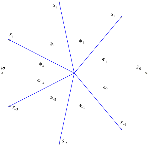
Figure 5.1. The jump contour $\gamma$ for the RH problem 1 and canonical solutions $\Phi_{j}(\lambda)$, $j=-3,-2,\dots,3,4$.

5.2.1. Uniqueness of the solution to the RH problem 1

The solution of the RH problem 1 is unique. Indeed, the scalar function $\det\Phi^{(\nu)}(\lambda)$ is continuous across the set of rays $\gamma$ and is bounded at the origin. Therefore, $\det\Phi^{(\nu)}(\lambda)$ is an entire function, and taking into account (5.8) and applying the Liouville theorem, $\det\Phi^{(\nu)}(\lambda)\equiv-1$. Assume for the moment that there are two solutions of the RH problem 1, $\Phi^{(\nu)}(\lambda)$ and $\tilde{\Phi}^{(\nu)}(\lambda)$. Consider their ratio, $\chi(\lambda)=(\begin{smallmatrix}a&b\\ c&d\end{smallmatrix})=\tilde{\Phi}^{(\nu)}(\lambda)(\Phi^{(\nu)}(\lambda))^{-1}$. As it is easy to see, $\chi(\lambda)$ is continuous across all the rays of the set $\gamma$ and is bounded at the origin, thus $\chi(\lambda)$ is an entire function. Using (5.8),

$$\lim_{\lambda\to\infty}\lambda^{-\frac{\nu}{4}\sigma_{3}}\chi(\lambda)\lambda^{\frac{\nu}{4}\sigma_{3}}=\lim_{\lambda\to\infty}\begin{pmatrix}a&b\lambda^{-\nu/2}\\ c\lambda^{\nu/2}&d\end{pmatrix}=I.$$

Since all the entries $a,b,c,d$ are entire functions in $\lambda$, the Liouville theorem yields the ambiguity

$$\Phi^{(\nu)}(\lambda)\mapsto\tilde{\Phi}^{(\nu)}(\lambda)=P^{(\nu)}(\lambda)\Phi^{(\nu)}(\lambda),\\ P^{(-1)}(\lambda)=I+c_{0}\sigma_{-},\quad P^{(3)}(\lambda)=I+(c_{0}\lambda+c_{1})\sigma_{+},\\ P^{(-5)}(\lambda)=I+(c_{0}\lambda^{2}+c_{1}\lambda+c_{2})\sigma_{-},$$ (5.14)

where $c_{j}$ are arbitrary constants. These ambiguities however are eliminated using the asymptotic conditions in (5.9), (5.10) and (5.11).

5.3. Solvability of the RH problems 1 and the Malgrange divisor

Given jump matrices, the set of points $(x,t)$ at which the RH problem is not solvable is called the Malgrange divisor. It coincides with the zero locus of a holomorphic $\tau$-function by Miwa and with the singularity locus of the isomonodromy deformation equation.

For what follows, it is convenient to articulate our assumptions on the singularities and critical points of equations P${}_{\mbox{\rm\tiny I}}^{2}$ and P${}_{\mbox{\rm\tiny I}}^{(2,1)}$.

Conjecture 5.1.

1) Equation P${}_{\mbox{\rm\tiny I}}^{(2,2)}$ has no other movable singularities except for the movable poles (2.5) satisfying (2.6), (2.7), and their triple collisions (2.8). 2) Equation P${}_{\mbox{\rm\tiny I}}^{(2,1)}$ has no other movable singularities or critical points except for the branch points (4.1).

These assumptions mean that the smooth branches of the Malgrange divisor for the RH problem 1 with $\nu=-1$ (corresponding to P${}_{\mbox{\rm\tiny I}}^{(2,2)}$) are parameterized by equations $x=a(t)$ and thus coincide with the solvability set for the RH problem 1 with $\nu=3$ (corresponding to P${}_{\mbox{\rm\tiny I}}^{(2,1)}$). Similarly, the vertices of the Malgrange divisor of the RH problem with $\nu=-1$ correspond to the branch points $t=b$ of $a(t)$ and therefore coincide with the solvability set of the RH problem with $\nu=-5$.

In other words, Conjecture 5.1 implies the following remarkable properties of the domains of solvability of all three RH problems:

1. these domains do not pairwise intersect;

2. all these domains together cover the deformation parameter space ${\mathbb{C}}\times{\mathbb{C}}\ni(t,x)$.

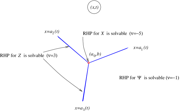
Figure 5.2. The scheme of the Malgrange divisor and the domains of the RH problems solvability for $\nu=-1,3,-5$.

5.4. Normalized non-homogeneous and homogeneous RH problems

In this section, we describe another interesting feature of the family of three RH problems. Roughly speaking, any solution of the non-homogeneous RH problem with the bigger value of $|\nu|$ allows one to construct infinitely many solutions of the homogeneous problems with the smaller value of $|\nu|$.

Precise formulation of this property requires some more accuracy. First of all, let us introduce the RH problems equivalent to those above but unbranched and normalized at infinity. To this aim, write

$$\lambda=\zeta^{4},\quad\hat{\Phi}^{(\nu)}_{k}(\zeta)=\tfrac{1}{\sqrt{2}}(\sigma_{3}+\sigma_{1})\zeta^{-4\nu\sigma_{3}}\Phi^{(\nu)}_{k}(\zeta^{4})e^{-\theta(\zeta^{4})},$$ (5.15)

and define the piece-wise holomorphic functions,

$$\hat{\Phi}^{(\nu)}(\zeta)=\hat{\Phi}^{(\nu)}_{k}(\zeta),\quad\arg\zeta\in\bigl{(}\tfrac{\pi}{14}(k-1),\tfrac{\pi}{14}k\bigr{)},\quad\nu=-1,3,-5.$$ (5.16)

These functions solve the non-homogeneous RH problems on the union of rays $\cup_{k=-13}^{14}\ell_{k}$, $\ell_{k}=\{\zeta\in{\mathbb{C}}\colon\ \arg\zeta=\tfrac{\pi}{14}k\}$ with a singular point at the origin and normalized to the unit at infinity. The corresponding homogeneous RH problem differs from the non-homogeneous counterpart in the asymptotics of $\Phi^{(\nu)}(\zeta)$ that vanishes as $\zeta\to\infty$.

Slightly abusing our notations, we formulate the non-homogeneous and homogeneous RH problems as follows:

Riemann–Hilbert problem 2.

Find a piece-wise holomorphic function $\hat{\Phi}_{I}^{(\nu)}(\zeta)$ $(\mbox{resp.,}\ \hat{\Phi}_{0}^{(\nu)}(\zeta))$, $\nu\in\{-1,3,-5\}$, with the following properties:

1. $\lim_{\zeta\to\infty}\hat{\Phi}_{I}^{(\nu)}(\zeta)=I$ $(\mbox{resp.,}\quad\lim_{\zeta\to\infty}\hat{\Phi}_{0}^{(\nu)}(\zeta)=0)$;

2. across the rays $\ell_{k}=\{\zeta\in{\mathbb{C}}\colon\arg\zeta=\tfrac{\pi}{14}k\}$, $k=-13,\dots,13,14$, all oriented towards infinity, the following jump conditions hold,

   $$\hat{\Phi}^{(\nu)}_{+}(\zeta)=\hat{\Phi}^{(\nu)}_{-}(\zeta)e^{\theta\sigma_{3}}S_{k}e^{-\theta\sigma_{3}},\quad\zeta\in\ell_{k},\quad\theta=\tfrac{1}{105}\zeta^{14}-\tfrac{1}{3}t\zeta^{6}+x\zeta^{2};$$ (5.17)

3. $\|\zeta^{\nu\sigma_{3}}\tfrac{1}{\sqrt{2}}(\sigma_{3}+\sigma_{1})\hat{\Phi}^{(\nu)}(\zeta)\|<const$, as $\zeta\to 0$.

The following theorem holds true

Theorem 5.1.

Any solution $\hat{\Phi}_{I}^{(3)}(\zeta)$ to the non-homogeneous RH problem 2 with $\nu=3$ yields infinitely many solutions $\hat{\Phi}_{0}^{(-1)}(\zeta)$ to the homogeneous RH problem 2 with $\nu=-1$. Any solution $\hat{\Phi}_{I}^{(-5)}(\zeta)$ to the non-homogeneous RH problem 2 with $\nu=-5$ yields infinitely many solutions $\hat{\Phi}_{0}^{(\nu)}(\zeta)$ to the homogeneous RH problem 2 with $\nu=3,-1$.

Proof.

We prove the first part of the theorem. The proof of the second part is similar.

Consider a solution $\hat{\Phi}_{I}^{(3)}(\zeta)$ to the RH problem 2 for $\nu=3$. It has the asymptotics

$$\hat{\Phi}_{I}^{(3)}(\zeta)=I+{\mathcal{O}}(\zeta^{-2}),\quad\zeta\to\infty,\\ \hat{\Phi}_{I}^{(3)}(\zeta)=\tfrac{1}{\sqrt{2}}(\sigma_{3}+\sigma_{1})\zeta^{-3\sigma_{3}}\bigl{(}M_{0}+{\mathcal{O}}(\zeta^{4})\bigr{)},\quad\zeta\to 0,\quad\zeta\in\omega_{0},\hfill$$

where $M_{0}$ is a constant matrix, $\det M_{0}\neq 0$, and $\omega_{0}=\{\zeta\in{\mathbb{C}}\colon\arg\zeta\in(0,\tfrac{\pi}{14})\}$. Then

$$\hat{\Phi}_{0}^{(-1)}(\zeta)=\zeta^{-2}N\hat{\Phi}_{I}^{(3)}(\zeta),\\ N=\tfrac{1}{\sqrt{2}}(\sigma_{3}+\sigma_{1})\begin{pmatrix}0&p\\ 0&q\end{pmatrix}\tfrac{1}{\sqrt{2}}(\sigma_{3}+\sigma_{1}),\quad p,q=const,$$

has the same jump properties as $\hat{\Phi}_{I}^{(3)}(\zeta)$ and the asymptotics of the form,

$$\hat{\Phi}_{0}^{(-1)}(\zeta)={\mathcal{O}}(\zeta^{-2}),\quad\zeta\to\infty,\\ \hat{\Phi}_{0}^{(-1)}(\zeta)=\tfrac{1}{\sqrt{2}}(\sigma_{3}+\sigma_{1})\zeta^{\sigma_{3}}\begin{pmatrix}0&p\\ 0&q\zeta^{2}\end{pmatrix}\bigl{(}M_{0}+{\mathcal{O}}(\zeta^{4})\bigr{)},\quad\zeta\to 0,\quad\zeta\in\omega_{0}.\hfill$$

Thus $\hat{\Phi}_{0}^{(-1)}(\zeta)$ is the solution of the homogeneous RH problem 2 with $\nu=-1$. ∎

6. Large $t$ asymptotics of a special solution of equations P${}_{\mbox{\rm\tiny I}}^{2}$ and P${}_{\mbox{\rm\tiny I}}^{(2,1)}$

In this section, we construct large $t$ asymptotic solution to the RH problem 1 for $\nu=-1$ and $\nu=3$ corresponding to a special solution of equation P${}_{\mbox{\rm\tiny I}}^{2}$. This special solution $u(x,t)$ has the asymptotics $u\sim\mp\sqrt[3]{6|x|}$ as $x\to\pm\infty$ and is real and regular on the real line for any $t\in\mathbb{R}$. The physical importance of this solution for $t=0$ from the point of view of string theory was justified in [3]. In [11, 12], this solution appeared in the study of the problem of universality of critical behavior of solutions to Hamiltonian perturbations of hyperbolic PDEs.

The above mentioned properties uniquely distinguish this special solution. In [26], the characterization of this solution in terms of the Stokes multipliers of the associated linear system was found,

$$s_{-2}=s_{-1}=s_{1}=s_{2}=0,\quad s_{-3}=s_{0}=s_{3}=-i.$$ (6.1)

6.1. Large $t$ asymptotic spectral curve for the special solution to P${}_{\mbox{\rm\tiny I}}^{2}$

Assume that $t>0$ is large and $x\in{\mathbb{C}}$ is such that

$$x_{0}:=xt^{-3/2}={\mathcal{O}}(1)\quad\mbox{as}\quad t\to+\infty.$$ (6.2)

Our starting point is the large $t$ asymptotics of the spectral curve, $\det(\mu-t^{-5/4}A(\lambda))=0$, where $\lambda=t^{1/2}\xi$, i.e.

$$\mu^{2}=\tfrac{1}{900}\xi^{5}-\tfrac{1}{30}\xi^{3}+\tfrac{1}{30}x_{0}\xi^{2}+\tfrac{1}{30}D_{1}\xi+\tfrac{1}{30}D_{0}=\tfrac{1}{900}\prod_{k=1}^{5}(\xi-\xi_{k}).$$ (6.3)

The asymptotic analysis of various degenerated solutions of P${}_{\mbox{\rm\tiny I}}^{2}$ performed in [20], shows that the topological properties of the asymptotic spectral curve are significantly different in the interior of the domains $D_{\pm}$ and $D_{0}$, see Figure 6.1. For $x_{0}\in D_{\pm}$, the spectral curve has genus 0,

$$\mu^{2}=\tfrac{1}{900}(\xi-\xi_{i})^{2}(\xi-\xi_{j})^{2}(\xi-\xi_{k}),$$ (6.4)

where the double branch points $\xi_{i},\xi_{j}$ and the simple branch point $\xi_{k}$ satisfy the conditions,

$$\xi_{i,j}=-\tfrac{1}{4}\xi_{k}\pm\sqrt{15-\tfrac{5}{16}\xi_{k}^{2}},\quad\xi_{k}^{3}-24\xi_{k}+48x_{0}=0,$$

and the ambiguity in choice of the root of the cubic equation for the simple branch point $\xi_{k}$ is fixed demanding that, for $x_{0}\in{\mathbb{R}}$,

$$\mbox{\,\rm sgn}(x_{0})\,\mbox{\rm Re}\,\Bigl{(}\int_{\xi_{k}}^{\xi_{i,j}}\mu(z)\,dz\Bigr{)}>0,\quad x_{0}\to\pm\infty.$$

The conditions above are consistent with the quasi-stationary asymptotic behavior of the special solution to P${}_{\mbox{\rm\tiny I}}^{2}$ (2.1),

$$u(x,t)\simeq t^{1/2}v_{0},\quad v_{0}^{3}-6v_{0}+6x_{0}=0,\\ v_{0}\simeq-\sqrt[3]{6x_{0}},\quad x_{0}\to\pm\infty,$$ (6.5)

where the real on the real line branch of $\sqrt[3]{6x_{0}}$ is chosen.

Figure 6.1. The discriminant set for the special solution of equation P${}_{\mbox{\rm\tiny I}}^{2}$. In the interior of the domains $D_{+}$ and $D_{-}$, the asymptotics of the special solution has genus $g=0$, and in the domain $D_{0}$, it has genus $g=1$.

Let us indicate some interesting points in the $x_{0}$ complex plane.

At the point $x_{0}=-2\sqrt{3}=D_{0}\cap D_{-}\cap{\mathbb{R}}$, two double branch points of the asymptotic spectral curve coalesce, so that $\xi_{1,2,3,4}=-\sqrt{3}$ and $\xi_{5}=4\sqrt{3}$. Generically, at the asymptotically quadruple branch point, the local solution of the RH problem can be approximated using the Garnier–Jimbo–Miwa $\Psi$ function for the second Painlevé transcendent P${}_{\mbox{\rm\tiny II}}$, [19, 25]. For the RH problem we are studying, the relevant local approximate solution corresponds to a Hastings–McLeod solution to P${}_{\mbox{\rm\tiny II}}$ [6].

At any $x_{0}\in D_{+}$ including its boundary, the spectral curve has one simple and two double branch points. The precise asymptotic location of these branch points can be found for $x_{0}=\tfrac{2\sqrt{5}}{9\sqrt{3}}=D_{0}\cap D_{+}\cap{\mathbb{R}}$, where $\xi_{3}=-\tfrac{4\sqrt{5}}{\sqrt{3}}$, $\xi_{1,2}=-\tfrac{\sqrt{5}}{\sqrt{3}}$ and $\xi_{4,5}=\tfrac{3\sqrt{5}}{\sqrt{3}}$. At this point, as well as at any point of $D_{+}$ including its boundary, the leading order asymptotic solution of the RH problem can be expressed in elementary functions, cf. [4] for the real line case.

Observe also the point $x_{0}=2\sqrt{3}\in D_{+}$ where two double branch points coalesce. The asymptotic branch points corresponding to this point are $\xi_{3}=-4\sqrt{3}$ and $\xi_{1,2,4,5}=\sqrt{3}$. Generically, the quadruple degeneration corresponds to the appearance of P${}_{\mbox{\rm\tiny II}}$. However, for the RH problem we consider here, the relevant Painlevé function is trivial, and the asymptotic solution to the RH problem remains elementary.

In the interior part of the domain $D_{0}$, the large $t$ asymptotic solution to the RH problem is constructed on the model elliptic curve,

$$\mu^{2}=\tfrac{1}{900}(\xi-\xi_{1})^{2}(\xi-\xi_{3})(\xi-\xi_{4})(\xi-\xi_{5}),$$ (6.6)

where the branch points $\xi_{j}$, $j=3,4,5$, are determined by the values of $\xi_{1}$ and $x_{0}$ as the roots of the cubic equation

$$\xi^{3}+2\xi_{1}\xi^{2}+(3\xi_{1}^{2}-30)\xi+4\xi_{1}^{3}-60\xi_{1}+30x_{0}=0.$$ (6.7)

The double branch point $\xi_{1}$ is determined as a function of $x_{0}\in D_{0}$ by the system of Boutroux equations, see [27],

$$\mbox{\rm Re}\,\int_{\xi_{3}}^{\xi_{4}}\mu(z)\,dz=0,\quad\mbox{\rm Re}\,\int_{\xi_{4}}^{\xi_{5}}\mu(z)\,dz=0,$$ (6.8)

supplemented by the described above boundary conditions on $D_{\pm}\cap D_{0}$.

Remark 6.1.

As $x_{0}$ approaches the real segment $(-2\sqrt{3},\tfrac{2\sqrt{5}}{9\sqrt{3}})$, all asymptotic branch points become real and satisfy the inequalities $\xi_{3}<\xi_{1}<\xi_{4}<\xi_{5}$. Thus the second of the equations (6.8) trivializes while the first of these equations turns into the condition $\int_{\xi_{3}}^{\xi_{4}}\mu(z)\,dz=0$ obtained in [36] in the analysis of the Whitham equations and used in [4] to study the same special solution on the real line.

6.2. Steepest-descent analysis of the RH problem

The strategy of the steepest-descent asymptotic analysis by Deift and Zhou [9, 10] of the RH problem involves several standard steps: 1) transformation of the jump graph to the steepest-descent directions of a suitable $g$-function; 2) construction of the local approximate solutions (parametrices); 3) matching all the parametrices into a global parametrix; 4) proof that the global parametrix indeed approximates the genuine solution to the original RH problem.

Since all the above mentioned steps are well explained in the literature (see e.g. [13]), below, we omit unnecessary details.

6.2.1. Transformation of the jump graph to the steepest-descent directions

According the steepest-descent strategy, we first transform the jump contour for each of the RH problems to the steepest-descent graph for the exponential $\exp\{\int^{\xi}\mu(z)\,dz\}$, see Figure 6.2.

Figure 6.2. Typical anti-Stokes lines for the special solution of P${}_{\mbox{\rm\tiny I}}^{2}$ as $x_{0}\in D_{0}$, $\mbox{\rm Im}\,x_{0}>0$.

Observe that, in the special case (6.1), $s_{\pm 2}=s_{\pm 1}=0$, $s_{0}=s_{\pm 3}=-i$, the jump graph depicted on Figure 5.1 can be transformed to the one shown in Figure 6.3,

Figure 6.3. The jump graph for the RH problem in the special case $s_{\pm 2}=s_{\pm 1}=0$, $s_{0}=s_{\pm 3}=-i$.

where

$$\Sigma_{-}:=\begin{pmatrix}1&0\\ -i&1\end{pmatrix},\quad\Sigma_{+}:=\begin{pmatrix}1&-i\\ 0&1\end{pmatrix}.$$ (6.9)

6.2.2. Model elliptic curve and abelian integrals

The large $t$ asymptotics of $\Psi(\lambda)$ corresponding to the Stokes multipliers (6.1) is constructed on the Riemann surface $\Gamma$ of the model elliptic curve

$$w^{2}=(\xi-\xi_{3})(\xi-\xi_{4})(\xi-\xi_{5}),$$ (6.10)

glued of two copies of the complex $\xi$-plane cut along $[\xi_{5},\xi_{4}]\cup[\xi_{3},-\infty)$, see Figure 6.4.

Figure 6.4. The Riemann surface $\Gamma$ and the basis of cycles $a,b$.

Define the complete elliptic integrals

$${\mathcal{A}},{\mathcal{B}}=\oint_{a,b}\mu(\xi)\,d\xi=\tfrac{1}{30}\oint_{a,b}(\xi-\xi_{1})w(\xi)\,d\xi,\\ \omega_{a,b}=\oint_{a,b}\frac{d\xi}{w(\xi)},\quad\tau=\frac{\omega_{b}}{\omega_{a}},\quad\mbox{\rm Im}\,\tau>0,\hfill$$ (6.11)

and abelian integrals

$$g(\xi)=\int_{\xi_{5}}^{\xi}\mu(z)\,dz,\quad U(\xi)=\frac{1}{\omega_{a}}\int_{\xi_{5}}^{\xi}\frac{dz}{w(z)}.$$ (6.12)

We define the integral $g(\xi)$ on the upper sheet of the Riemann surface $\Gamma$ cut along the sum of intervals $[\xi_{5},\xi_{4}]\cup[\xi_{4},\xi_{3}]\cup[\xi_{3},-\infty)$.

The Boutroux conditions (6.8) imply

$${\mathcal{A}},{\mathcal{B}}\in i{\mathbb{R}}.$$ (6.13)

Observe the following properties of $g(\xi)$ and $U(\xi)$:

1. as $\xi\to\infty$,

   $$U(\xi)=U_{\infty}+{\mathcal{O}}(\xi^{-1/2}),\quad U_{\infty}=-\tfrac{1}{2}\tau,\\ g(\xi)=\vartheta+g_{\infty}+{\mathcal{O}}(\xi^{-1/2}),\quad\vartheta=\tfrac{1}{105}\xi^{7/2}-\tfrac{1}{3}\xi^{3/2}+x_{0}\xi^{1/2},\quad g_{\infty}=-\tfrac{1}{2}{\mathcal{B}},\hfill$$ (6.14)

2. $g(\xi)$ and $U(\xi)$ are discontinuous across the broken line $[\xi_{5},\xi_{4}]\cup[\xi_{4},\xi_{3}]\cup[\xi_{3},-\infty)$ oriented from $\xi_{5}$ to infinity, moreover

   $$\xi\in(\xi_{5},\xi_{4})\colon\quad g_{+}(\xi)+g_{-}(\xi)=0,\quad U_{+}(\xi)+U_{-}(\xi)=0,\\ \xi\in(\xi_{4},\xi_{3})\colon\quad g_{+}(\xi)-g_{-}(\xi)=-{\mathcal{A}},\quad U_{+}(\xi)-U_{-}(\xi)=-1,\hfill\\ \xi\in(\xi_{3},\infty)\colon\quad g_{+}(\xi)+g_{-}(\xi)=-{\mathcal{B}},\quad U_{+}(\xi)+U_{-}(\xi)=-\tau.\hfill\\$$ (6.15)

6.3. “External” parametrix

In this subsection, following [13], we solve the permutation RH problem on the segments $[\xi_{5},\xi_{4}]\cup[\xi_{3},-\infty)$ whose solution gives a leading order contribution to the solution of the above RH problem.

Riemann–Hilbert problem 3.

Given $t\gg 1$ and the complex value of the parameter $x_{0}$, find a piece-wise holomorphic $2\times 2$ matrix function $\Phi^{(\nu)}(\xi)$ with the following properties:

$$\hskip 0.0pt(1)\qquad\lim_{\xi\to\infty}\tfrac{1}{\sqrt{2}}(\sigma_{3}+\sigma_{1})\xi^{-\frac{\nu}{4}\sigma_{3}}t^{-\frac{\nu}{8}\sigma_{3}}\Phi^{(\nu)}(\xi)e^{-t^{7/4}\vartheta\sigma_{3}}=I,$$ (6.16)

where

$$\vartheta=\tfrac{1}{105}\xi^{7/2}-\tfrac{1}{3}\xi^{3/2}+x_{0}\xi^{1/2};$$ (6.17)

across the union of segments $(\xi_{5},\xi_{4})\cup(\xi_{3},-\infty)$ oriented as indicated, the jump condition holds true,

$$\Phi^{(\nu)}_{+}(\xi)=\Phi^{(\nu)}_{-}(\xi)i\sigma_{1},\quad\xi\in(\xi_{5},\xi_{4})\cup(\xi_{3},-\infty)$$ (6.18)

where $\Phi^{(\nu)}_{+}(\xi)$ and $\Phi^{(\nu)}_{-}(\xi)$ are limits of $\Phi^{(\nu)}(\xi)$ on the segments from the left and from the right, respectively, see Figure 6.3.

We do not impose any conditions on the behavior of $\Phi^{(\nu)}(\xi)$ at the points $\xi=\xi_{j}$, $j=3,4,5$. As the result, the solution of the model RH problem 3 is determined up to a left rational matrix multiplier with possible poles at $\xi=\xi_{j}$, $j=3,4,5$, and certain asymptotics at infinity. Below, we will use this rational multiplier to prove or disprove the asymptotic solvability of the original RH problem 1.

6.3.1. $\beta$-factor

Consider the principal branches of the functions $\beta_{\nu}(\xi)$,

$$\beta_{-1}(\xi)=(\xi-\xi_{3})^{-1/4}(\xi-\xi_{4})^{1/4}(\xi-\xi_{5})^{-1/4}$$ (6.19)

$$\beta_{3}(\xi)=(\xi-\xi_{3})^{1/4}(\xi-\xi_{4})^{1/4}(\xi-\xi_{5})^{1/4}$$ (6.20)

both defined on the $\xi$ complex plane with cuts along the broken line $[\xi_{5},\xi_{4}]\cup[\xi_{4}\xi_{3}]\cup[\xi_{3},-\infty)$. These functions solve the scalar RH problems:

1. $\beta_{\nu}(\xi)=\xi^{\frac{\nu}{4}}(1+{\mathcal{O}}(\xi^{-1}))$, as $\xi\to\infty$;

2. the discontinuity of $\beta_{\nu}(\xi)$ across the oriented contour $[\xi_{5},\xi_{4}]\cup[\xi_{4}\xi_{3}]\cup[\xi_{3},-\infty)$ is described by the conditions

   $$\xi\in(\xi_{5},\xi_{4})\colon\quad\beta_{-1}^{+}(\xi)=i\beta_{-1}^{-}(\xi),\quad\beta_{3}^{+}(\xi)=-i\beta_{3}^{-}(\xi),\\ \xi\in(\xi_{4},\xi_{3})\colon\quad\beta_{-1}^{+}(\xi)=\beta_{-1}^{-}(\xi),\quad\beta_{3}^{+}(\xi)=-\beta_{3}^{-}(\xi),\hfill\\ \xi\in(\xi_{3},-\infty)\colon\quad\beta_{-1}^{+}(\xi)=i\beta_{-1}^{-}(\xi),\quad\beta_{3}^{+}(\xi)=i\beta_{3}^{-}(\xi).\hfill$$ (6.21)

6.3.2. The Riemann theta function and the Baker–Akhiezer functions

Define one more function,

$$h_{\nu}(\xi)=t^{7/4}(g(\xi)-g_{\infty})+\delta_{\nu}(U(\xi)-U_{\infty}),\quad g_{\infty}=-\tfrac{1}{2}{\mathcal{B}},\quad U_{\infty}=-\tfrac{1}{2}\tau,$$ (6.22)

where the parameter $\delta_{\nu}$ is defined by

$$\delta_{-1}=-t^{7/4}{\mathcal{A}},\quad\delta_{3}=-t^{7/4}{\mathcal{A}}+i\pi.$$ (6.23)

This function $h_{\nu}(\xi)$ has the following obvious properties,

(1) as $\xi\to+\infty$,

$$h_{\nu}(\xi)=t^{7/4}\vartheta+{\mathcal{O}}(\xi^{-1/2});$$ (6.24)

(2) $h_{\nu}(\xi)$ is discontinuous across the broken line $[\xi_{5},\xi_{4}]\cup[\xi_{4},\xi_{3}]\cup[\xi_{3},-\infty)$ oriented from $\xi_{5}$ to infinity, moreover

$$\xi\in(\xi_{5},\xi_{4})\colon\quad h_{\nu}^{+}(\xi)+h_{\nu}^{-}(\xi)=t^{7/4}{\mathcal{B}}+\delta_{\nu}\tau,\\ \xi\in(\xi_{4},\xi_{3})\colon\quad h_{\nu}^{+}(\xi)-h_{\nu}^{-}(\xi)=-t^{7/4}{\mathcal{A}}-\delta_{\nu},\hfill\\ \xi\in(\xi_{3},\infty)\colon\quad h_{\nu}^{+}(\xi)+h_{\nu}^{-}(\xi)=0.\hfill$$ (6.25)

Using the Riemann theta-function, $\Theta(z)=\sum_{n}e^{\pi in^{2}\tau+2\pi inz}$, define the matrix function $\Phi_{\nu}^{(BA)}(\xi)$,

$$\Phi_{\nu}^{(BA)}(\xi)=(\beta_{\nu}(\xi))^{\sigma_{3}}\tfrac{1}{\sqrt{2}}\times\\ \times\begin{pmatrix}\tfrac{\Theta(U(\xi)+V+\phi_{\nu})}{\Theta(U(\xi)+\frac{1+\tau}{2})}c_{1}(\xi)&\tfrac{\Theta(-U(\xi)+V+\phi_{\nu})}{\Theta(-U(\xi)+\frac{1+\tau}{2})}c_{1}^{*}(\xi)\\ \tfrac{\Theta(U(\xi)+V+\phi_{\nu}-\frac{1+\tau}{2})}{\Theta(U(\xi))}c_{2}(\xi)&\tfrac{\Theta(-U(\xi)+V+\phi_{\nu}-\frac{1+\tau}{2})}{\Theta(-U(\xi))}c_{2}^{*}(\xi)\end{pmatrix}e^{h_{\nu}(\xi)\sigma_{3}}.$$ (6.26)

Here the parameters $V$, $\phi_{\nu}$ and the factors $c_{j}(\xi)$, $c_{j}^{*}(\xi)$ are defined by

$$V=-\tfrac{1}{2\pi i}t^{7/4}(\tau{\mathcal{A}}-{\mathcal{B}});\\ \phi_{-1}=\tfrac{1+\tau}{2},\quad\phi_{3}=0;\\ c_{1}(\xi)=\tfrac{\Theta(\frac{1}{2})}{\Theta(V+\phi_{\nu}-\frac{\tau}{2})},\quad c_{1}^{*}(\xi)=\tfrac{\Theta(\frac{1}{2}+\tau)}{\Theta(V+\phi_{\nu}+\frac{\tau}{2})}\quad\mbox{if}\quad V+\phi_{\nu}\neq\tfrac{1}{2}+n+m\tau,\\ c_{1}(\xi)=\beta_{-1}^{-2}(\xi)\tfrac{\omega_{a}\Theta(\frac{1}{2})}{2\Theta^{\prime}(\frac{1+\tau}{2})},\quad c_{1}^{*}(\xi)=\beta_{-1}^{-2}(\xi)\tfrac{\omega_{a}\Theta(\frac{1}{2}+\tau)}{2\Theta^{\prime}(\tfrac{1+\tau}{2})}\quad\mbox{if}\quad V+\phi_{\nu}=\tfrac{1}{2},\hfill\\ c_{2}(\xi)=\tfrac{\Theta(\frac{\tau}{2})}{\Theta(V+\phi_{\nu}-\frac{1}{2}-\tau)},\quad c_{2}^{*}(\xi)=\tfrac{\Theta(\frac{\tau}{2})}{\Theta(V+\phi_{\nu}-\frac{1}{2})}\quad\mbox{if}\quad V+\phi_{\nu}\neq\tfrac{\tau}{2}+n+m\tau,\\ c_{2}(\xi)=\beta_{-1}^{-2}(\xi)\tfrac{\omega_{a}\Theta(\frac{\tau}{2})}{2\Theta^{\prime}(\frac{1+\tau}{2})},\quad c_{2}^{*}(\xi)=\beta_{-1}^{-2}(\xi)\tfrac{\omega_{a}\Theta(\frac{\tau}{2})}{2\Theta^{\prime}(\frac{1+\tau}{2})}\quad\mbox{if}\quad V+\phi_{\nu}=\tfrac{\tau}{2},\hfill\\ n,m\in{\mathbb{Z}}.$$ (6.27)

It can be shown that $\det\Phi_{\nu}^{(BA)}(\xi)\equiv-1$, the function $\Phi_{\nu}^{(BA)}(\xi)$ (6.26) satisfies (6.16) and (6.18) and thus is one of the solutions of the RH problem 3. Any other solution to this RH problem has the form of the product

$$\Psi_{\nu}^{(BA)}(\xi)=R_{\nu}(\xi)\Phi_{\nu}^{(BA)}(\xi),$$ (6.28)

where $R_{\nu}(\xi)$ is rational with poles at $\xi=\xi_{j}$, $j=3,4,5$, and satisfies the asymptotic condition $R_{\nu}(\xi)=I+{\mathcal{O}}(\xi^{-1})$ as $\xi\to\infty$.

6.4. Local RH problem solution near the branch points $\xi=\xi_{j}$, $j=5,4,3$

As it is well known, near a single branch points, the relevant boundary-value problem can be solved using the classical Airy functions, see e.g. [13].

6.4.1. RH problem for the Airy functions

Define the Wronsky matrix of the Airy functions [1],

$$Z_{0}(z)=\sqrt{2\pi}e^{-i\pi/4}\begin{pmatrix}v_{2}(z)&v_{1}(z)\\ \frac{d}{dz}v_{2}(z)&\frac{d}{dz}v_{1}(z)\end{pmatrix}e^{-i\pi\sigma_{3}/4},$$ (6.29)

where

$$v_{1}(z)=\mbox{\rm Ai}\,(z),\quad v_{2}(z)=e^{i2\pi/3}\mbox{\rm Ai}\,(e^{i2\pi/3}z).$$ (6.30)

Besides $Z_{0}(z)$, introduce auxiliary functions

$$Z_{-1}(z)=Z_{0}(z)(\Sigma_{+})^{-1},\quad Z_{1}(z)=Z_{0}(z)\Sigma_{-},\quad Z_{2}(z)=Z_{1}(z)\Sigma_{+},\\ \Sigma_{+}=\begin{pmatrix}1&-i\\ 0&1\end{pmatrix},\quad\Sigma_{-}=\begin{pmatrix}1&0\\ -i&1\end{pmatrix}.$$ (6.31)

By construction [1],

$$Z_{j}(z)=z^{-\sigma_{3}/4}\tfrac{1}{\sqrt{2}}(\sigma_{3}+\sigma_{1})(I+{\mathcal{O}}(z^{-\frac{3}{2}}))e^{\frac{2}{3}z^{3/2}\sigma_{3}},\\ z\to\infty,\quad z\in\omega_{j}=\bigl{\{}z\in{\mathbb{C}}\colon\ \arg z\in\bigl{(}-\pi+\tfrac{2\pi}{3}j,\tfrac{\pi}{3}+\tfrac{2\pi}{3}j)\bigr{\}}.$$ (6.32)

Assemble the piece-wise holomorphic functions $Z^{(j)}(z)$, $j=5,4,3$,

$$Z^{(j)}(z)=\begin{cases}Z_{-1}(z)G_{j},\quad\arg z\in(-\pi,-\tfrac{2\pi}{3}),\\ Z_{0}(z)G_{j},\quad\arg z\in(-\tfrac{2\pi}{3},0),\\ Z_{1}(z)G_{j},\quad\arg z\in(0,\tfrac{2\pi}{3}),\\ Z_{2}(z)G_{j},\quad\arg z\in(\tfrac{2\pi}{3},\pi),\end{cases}$$ (6.33)

where

$$G_{5}=G_{3}=I,\quad G_{4}=i\sigma_{3}.$$

Observing that the jump matrices of $Z^{(j)}(z)$ coincide with those across the lines emanating from the node points $\xi_{j}$, $j=5,4,3$, in Figure 6.3, we are ready to construct the relevant local parametrices,

$$\Psi_{\nu}^{(j)}(\xi)=B^{(\nu)}_{j}(\xi)Z^{(j)}(z^{(j)}(\xi)),\quad j=5,4,3,\quad\nu=-1,3.$$ (6.34)

Here $B^{(\nu)}_{j}(\xi)$, $j=5,4,3$, are holomorphic in some finite neighborhoods of $\xi=\xi_{j}$ matrices, and $z=z^{(j)}(\xi)$ are changes of variables biholomorphic in some finite neighborhoods of $\xi=\xi_{j}$.

6.4.2. Determination of the local change $z=z^{(j)}(\xi)$

This biholomorphic change of variables has to be chosen in a way to ensure that the global parametrix, see below, has small enough jumps as $t\to+\infty$, namely it must satisfy the condition

$$\tfrac{2}{3}(z^{(j)}(\xi))^{3/2}=t^{7/4}(g(\xi)-g(\xi_{j}))+\delta_{\nu}(U(\xi)-U(\xi_{j}))+o(1),\quad|\xi-\xi_{j}|=const.$$

The biholomorphicity condition is satisfied with the choice

$$z^{(j)}(\xi)=t^{7/6}\Bigl{(}\tfrac{3}{2}\int_{\hat{\xi}_{j}}^{\xi}\hat{\mu}(z)\,dz\Bigr{)}^{2/3},\quad j=5,4,3,$$ (6.35)

where $\hat{\mu}(\xi)$ has the form (6.3), (6.6) with the branch points $\hat{\xi}_{j}$,

$$\hat{\mu}^{2}=\tfrac{1}{900}\xi^{5}-\tfrac{1}{30}\xi^{3}+\tfrac{1}{30}x_{0}\xi^{2}+\tfrac{1}{30}\hat{D}_{1}\xi+\tfrac{1}{30}\hat{D}_{0}=\\ =\tfrac{1}{900}(\xi-\hat{\xi}_{1})^{2}(\xi-\hat{\xi}_{3})(\xi-\hat{\xi}_{4})(\xi-\hat{\xi}_{5}).$$

The unique abelian differential holomorphic on the elliptic curve $\hat{w}^{2}=(\xi-\hat{\xi}_{3})(\xi-\hat{\xi}_{4})(\xi-\hat{\xi}_{5})$ is

$$d\hat{U}=\tfrac{2}{\hat{\omega}_{a}}\Bigl{(}\tfrac{\partial}{\partial\hat{D}_{1}}-\hat{\xi}_{1}\,\tfrac{\partial}{\partial\hat{D}_{0}}\Bigr{)}\hat{\mu}(\xi)\,d\xi.$$

Thus the 1-parameter deformation of the model degenerated curve that respects the degeneration is generated by the vector field

$$\tfrac{\partial}{\partial D}=\tfrac{2}{\hat{\omega}_{a}}\Bigl{(}\tfrac{\partial}{\partial\hat{D}_{1}}-\hat{\xi}_{1}\,\tfrac{\partial}{\partial\hat{D}_{0}}\Bigr{)}.$$ (6.36)

Finally, we find the elliptic curve satisfying the asymptotic conditions,

$$\mu(\xi)+t^{-7/4}\frac{\delta_{\nu}}{w(\xi)}=\hat{\mu}(\xi)+{\mathcal{O}}(t^{-7/2}(\xi-\xi_{j})^{-3/2}),\\ \mbox{as}\quad|\xi-\xi_{1}|>C_{1}t^{-7/8},\quad|\xi-\xi_{j}|>C_{j}t^{-7/4},\quad C_{j}=const,\quad j=3,4,5,\\ \omega_{a,b}=\hat{\omega}_{a,b}+{\mathcal{O}}(t^{-7/2}),\quad\hat{\tau}=\tau+{\mathcal{O}}(t^{-7/2}),\hfill\\ {\mathcal{A}}+t^{-7/4}\delta_{\nu}=\hat{\mathcal{A}}+{\mathcal{O}}(t^{-7/2}),\quad{\mathcal{B}}+t^{-7/4}\tau\delta_{\nu}=\hat{\mathcal{B}}+{\mathcal{O}}(t^{-7/2}).$$ (6.37)

6.5. Global parametrix

The global approximate solution to the RH problem for $\Phi^{(\nu)}(\xi)$, $\nu=-1,3$, is a piece-wise analytic matrix function $\tilde{\Psi}_{\nu}(\xi)$ defined as follows,

$$\tilde{\Psi}_{\nu}(\xi)=\begin{cases}\Psi_{\nu}^{(j)}(\xi),\quad\xi\in C_{j},\\ \Psi_{\nu}^{(BA)},\quad\xi\in{\mathbb{C}}\backslash\cup_{j}C_{j},\end{cases}\\ \Psi_{\nu}^{(BA)}(\xi)=R_{\nu}(\xi)\Phi^{(BA)}(\xi),\quad C_{j}=\{\xi\in{\mathbb{C}}\colon|\xi-\xi_{j}|<r\},\\ 0<r<\tfrac{1}{2}\min_{k\neq j}|\xi_{k}-\xi_{j}|,\quad k,j=3,4,5,$$ (6.38)

see Figure 6.5.

Figure 6.5. The construction of the global parametrix.

The exact solution is constructed using the correction function $\chi(\xi)$,

$$\chi(\xi)=\Psi(\xi)\tilde{\Psi}^{-1}(\xi),$$ (6.39)

that satisfies the following RH problem:

(1) the limit

$$\lim_{\xi\to\infty}\xi^{1/2}\bigl{(}\tfrac{1}{\sqrt{2}}(\sigma_{3}+\sigma_{1})\xi^{\frac{1}{4}\sigma_{3}}t^{\frac{1}{8}\sigma_{3}}\chi(\xi)t^{-\frac{1}{8}\sigma_{3}}\xi^{-\frac{1}{4}\sigma_{3}}\tfrac{1}{\sqrt{2}}(\sigma_{3}+\sigma_{1})-I\bigr{)}$$

exists and is diagonal;

(2) across the contour $\gamma$ shown in Figure 6.6, the jump condition holds, $\chi_{+}(\xi)=\chi_{-}(\xi)H(\xi)$ where

$$H(\xi)=\tilde{\Psi}_{-}(\xi)S(\xi)\tilde{\Psi}_{+}^{-1}(\xi).$$

Figure 6.6. The jump contour $\gamma$ for the correction function $\chi(\xi)$.

To apply the $L^{2}$-theory to the latter RH problem [43], all jump matrices $H(\xi)$ across the jump contour $\gamma$ in Figure 6.6 must satisfy the estimate $\|H(\xi)-I\|_{L^{2}(\gamma)\cap C(\gamma)}=o(1)$ as $t\to\infty$. For the infinite tails emanating from the circles, this fact holds true because the relevant jumps are uniformly exponentially small.

The jumps across the circles centered at the branch points $\xi_{j}$, $j=3,4,5$, can be made small as $t$ is large if one adjusts the rational matrix $R_{\nu}(\xi)$, $\nu=-1,3$, and the holomorphic matrices $B_{j}^{(\nu)}(\xi)$, $\nu=-1,3$, $j=5,4,3$, in an appropriate way. Omitting the straightforward but tedious computations, we present the result:

$$V-\tfrac{1}{2},V-\tfrac{\tau}{2},V-\tfrac{1+\tau}{2}\neq n+m\tau,\quad n,m\in{\mathbb{Z}}\colon\\ R_{-1}(\xi)=t^{-\frac{1}{8}\sigma_{3}}\begin{pmatrix}1&\frac{1}{\xi-\xi_{5}}q^{(\infty)}\\ r^{(\infty)}&1+\frac{1}{\xi-\xi_{5}}q^{(\infty)}r^{(\infty)}\end{pmatrix},\\ q^{(\infty)}=-\tfrac{\omega_{a}}{2}(\xi_{5}-\xi_{4})\tfrac{e^{2\pi iV(t)}\Theta(V+\frac{1+\tau}{2})\Theta(V+\frac{\tau}{2})\Theta(\frac{1}{2})\Theta(0)}{\Theta(V+\frac{1}{2})\Theta(V)\Theta(\frac{\tau}{2})\Theta^{\prime}(\frac{1+\tau}{2})},\\ r^{(\infty)}-q^{(\infty)}=\tfrac{2\Theta(V)\Theta(V+\frac{1+\tau}{2})\Theta^{\prime}(\frac{1+\tau}{2})\Theta(0)}{\omega_{a}\Theta(V+\frac{1}{2})\Theta(V+\frac{\tau}{2})\Theta(\frac{1}{2})\Theta(\frac{\tau}{2})},\\ V=\tfrac{1}{2}\colon\quad R_{-1}(\xi)=t^{-\frac{1}{8}\sigma_{3}}\Bigl{(}\frac{\xi-\xi_{5}}{\xi-\xi_{4}}\Bigr{)}^{\sigma_{3}},\\ V=\tfrac{\tau}{2}\colon\quad R_{-1}(\xi)=t^{-\frac{1}{8}\sigma_{3}}.\hfill$$ (6.40)

The relevant correction function satisfies the estimates

$$\chi(\xi)-I=\begin{cases}{\mathcal{O}}(t^{-7/24}),\quad|\xi|<\mbox{const},\\ {\mathcal{O}}(t^{-7/24}\xi^{-1}),\quad|\xi|\to\infty,\end{cases}$$ (6.41)

in the domain of the parameter $x_{0}=xt^{-3/2}$ described by

$$|V-\tfrac{1+\tau}{2}-n-m\tau|>Ct^{-\frac{7}{24}+\epsilon},\quad n,m\in{\mathbb{Z}},\quad\epsilon=\mbox{const}>0.$$ (6.42)

6.6. Large $t$ asymptotics of the RH problem 1($\nu=3$)

In contrast, the computation of the left rational multiplier $R_{\nu}(\xi)$ for $\nu=3$ yields

$$R_{3}(\xi)=t^{\frac{3}{8}\sigma_{3}}I,$$ (6.43)

together with the additional condition,

$$\Theta(V)=0,$$ (6.44)

or, equivalently,

$$V=\tfrac{1+\tau}{2}+n+m\tau.$$ (6.45)

In this case, the “external” parametrix is elementary,

$$\Phi_{3}^{(BA)}(\xi)=(\beta_{3}(\xi))^{\sigma_{3}}\tfrac{1}{\sqrt{2}}(\sigma_{3}+\sigma_{1})e^{h_{3}(\xi)\sigma_{3}},$$ (6.46)

and the correction function $\chi(\xi)$ satisfies the estimates (6.41).

Remark 6.2.

The above computation shows that, as $t\to+\infty$, for each value of the deformation parameter $x$, $xt^{-3/2}\in D_{0}$, the RH problem 1 is solvable either with $\nu=-1$ or $\nu=3$. Thus there is no room for the solvability of the RH problem with $\nu=-5$. Therefore, at least in the large $t$ limit, the special solution to P${}_{\mbox{\rm\tiny I}}^{2}$ has no triple pole collisions and the corresponding solutions to P${}_{\mbox{\rm\tiny I}}^{(2,1)}$ have no branch points. The relevant Malgrange divisor consists of smooth branches only.

7. Pole asymptotic distribution

To compute the large $t$ asymptotic distribution of poles of the special solution to P${}_{\mbox{\rm\tiny I}}^{2}$, we use the phase shift given in (6.45) and the definition of $V$ in (6.27),

$$\tfrac{1}{2\pi i}t^{7/4}(\tau{\mathcal{A}}-{\mathcal{B}})=n+\tfrac{1}{2}+(m+\tfrac{1}{2})\tau.$$ (7.1)

Using the canonical dissection of the Riemann surface, the difference $\omega_{b}{\mathcal{A}}-\omega_{a}{\mathcal{B}}$ is expressed in terms of a single contour integral over the contour ${\mathcal{L}}$ depicted in Figure 7.1,

Figure 7.1. The contour for the canonical dissection of the elliptic curve $\Gamma$.

$$\omega_{b}{\mathcal{A}}-\omega_{a}{\mathcal{B}}=\omega_{a}\oint_{\mathcal{L}}U(z)\mu(z)\,dz.$$

Inflating the contour ${\mathcal{L}}$, we transform it to a contour encircling the infinite point which is a branch point of the curve. Then expanding the integrand at the infinity and using the residue theorem, we find

$$\tau{\mathcal{A}}-{\mathcal{B}}=\oint_{\mathcal{L}}(U(z)-U_{\infty})\mu(z)\,dz=-\tfrac{8\pi i}{7\omega_{a}}(3x_{0}+\tfrac{2}{3}\xi_{1}),$$ (7.2)

and the pole distribution formula (7.1) yields

$$3x_{0}+\tfrac{2}{3}\xi_{1}=\tfrac{7}{4}t^{-7/4}\bigl{(}(n+\tfrac{1}{2})\omega_{a}+(m+\tfrac{1}{2})\omega_{b}\bigr{)}.$$ (7.3)

Since $\xi_{1}$ is determined by $x_{0}$ via the Boutroux equations (6.8), equation (7.3) determines the pole position, $x_{0}^{(n,m)}=x_{n,m}t^{-3/2}$ as a transcendent function of two integers $(n,m)$. As $t\to+\infty$, the particular pole $x_{0}^{(n,m)}$ approaches the attracting point satisfying the equation

$$\xi_{1}(x_{0})=-\tfrac{9}{2}x_{0}.$$ (7.4)

7.1. Quasi-stationary solutions of equation P${}_{\mbox{\rm\tiny I}}^{(2,1)}$

Although it is not known how to solve the transcendent equation (7.4), the problem of finding the attractor to the pole distribution significantly simplifies observing that the pole attractors correspond to the quasi-stationary solutions of equation P${}_{\mbox{\rm\tiny I}}^{(2,1)}$,

$$a(t)=a_{\infty}t^{3/2}(1+{\mathcal{O}}(t^{-\epsilon})),\quad\epsilon>0.$$ (7.5)

Substituting (7.5) into P${}_{\mbox{\rm\tiny I}}^{(2,1)}$ (2.7), we find an algebraic equation for the parameter $a_{\infty}$,

$$a_{\infty}^{4}-\tfrac{236}{243}a_{\infty}^{2}+\tfrac{160}{2187}=0,$$ (7.6)

with the roots $a_{\infty}\in\{\pm\tfrac{2\sqrt{5}}{9\sqrt{3}},\pm\tfrac{2\sqrt{2}}{3}\}$. However only one of the roots,

$$a_{\infty}=\tfrac{2\sqrt{5}}{9\sqrt{3}},$$ (7.7)

is consistent with the described above properties of the large $t$ asymptotic spectral curve for the special solution of P${}_{\mbox{\rm\tiny I}}^{2}$. The linearization of equation P${}_{\mbox{\rm\tiny I}}^{(2,1)}$at the 0-parameter power series solution with the leading order term coefficient (7.7) has four linearly independent solutions. Two of them are exponential, $\sim\exp[\pm i\tfrac{2\sqrt{2}}{3}(\tfrac{5}{3})^{3/4}\tfrac{4}{7}t^{7/4}]$, and we set them aside. Two other solutions of the linearized equation, $\sim t^{-1/4}$ and $\sim t^{-1/4}\ln t$, are relevant to our quasi-stationary behavior of the poles. Using them, we form the 2-parameter series

$$a(t)=t^{3/2}\sum_{k=0}^{\infty}(t^{-\frac{7}{4}}\ln(t^{-\frac{7}{4}}))^{k}a_{k}(t),\quad a_{k}(t)=\sum_{l=0}^{\infty}a_{kl}t^{-\frac{7}{4}l},\\ a_{00}=\tfrac{2\sqrt{5}}{9\sqrt{3}},\\ a_{10},a_{01}\in{\mathbb{C}}\quad\mbox{are arbitrary},\\ a_{20}=-\tfrac{3\sqrt{15}}{784}a_{10}^{2},\quad a_{11}=-\tfrac{3\sqrt{15}}{392}(a_{01}-2a_{10})a_{10},\\ \hfill a_{02}=\tfrac{3\sqrt{3}(\sqrt{15}-50a_{01}^{2}+200a_{01}a_{10}+3130a_{10}^{2})}{7840\sqrt{5}},\\ a_{30}=\tfrac{1467}{307328}a_{10}^{3},\quad a_{21}=\tfrac{27}{307328}(163a_{01}+861a_{10})a_{10}^{2},\\ a_{12}=\tfrac{27}{9834496}(1907\tfrac{\sqrt{3}}{\sqrt{5}}+5216a_{01}^{2}+55104a_{01}a_{10}+233392a_{10}^{2})a_{10},\\ \hfill a_{03}=\tfrac{9}{3073280}(1630a_{01}^{3}+25830a_{01}^{2}a_{10}+218805a_{01}a_{10}^{2}+788362a_{10}^{3})\\ \hfill+\tfrac{9\sqrt{3}}{49172480\sqrt{5}}(28605a_{01}+258143a_{10}),\quad\\ \dots\hfill$$ (7.8)

Let us relate the free parameters $a_{01},a_{10}$ in (7.8) with the integers $n$ and $m$ in (7.3). Recall that, along the boundary $\partial D_{+}$, two branch points $\xi_{4}$ and $\xi_{5}$ of the asymptotic spectral curve coalesce. Namely, if $t\to+\infty$, the limiting values corresponding to the attracting point are

$$x_{0}^{*}=\tfrac{2\sqrt{5}}{9\sqrt{3}},\quad\xi_{3}^{*}=-\tfrac{4\sqrt{5}}{\sqrt{3}},\quad\xi_{1,2}^{*}=-\tfrac{\sqrt{5}}{\sqrt{3}},\quad\xi_{4,5}^{*}=\sqrt{15}.$$ (7.9)

The asymptotics of the branch points in the model elliptic spectral curve compatible with the expansion (7.8) is given by

$$\xi_{1}=\xi_{2}=-\tfrac{\sqrt{5}}{\sqrt{3}}+\tfrac{3}{4}(a_{01}+7a_{10}+a_{10}\ln(t^{-7/4}))t^{-7/4}+{\mathcal{O}}(t^{-7/2}\ln^{2}t),\\ \xi_{3}=-\tfrac{4\sqrt{5}}{\sqrt{3}}-\tfrac{6}{7}\bigl{(}a_{01}+4a_{10}+a_{10}\ln(t^{-7/4})\bigr{)}t^{-7/4}+{\mathcal{O}}(t^{-7/2}\ln^{2}t),\quad\\ \xi_{4,5}=\sqrt{15}\mp\sqrt{6}\sqrt[4]{15}\sqrt{a_{10}}\,t^{-7/8}\\ -\tfrac{9}{28}\bigl{(}a_{01}+11a_{10}+a_{10}\ln(t^{-7/4})\bigr{)}t^{-7/4}+{\mathcal{O}}(t^{-21/8}\ln^{2}t).$$ (7.10)

The asymptotics of the periods $\omega_{a,b}$ as $\xi_{5}-\xi_{4}\to 0$ have the forms

$$\omega_{a}=\tfrac{2\pi i}{\sqrt{\xi_{4}-\xi_{3}}}(1-\tfrac{\xi_{5}-\xi_{4}}{4(\xi_{4}-\xi_{3})}+{\mathcal{O}}((\xi_{5}-\xi_{4})^{2})),\\ \omega_{b}=\tfrac{2}{\sqrt{\xi_{4}-\xi_{3}}}\ln\tfrac{\xi_{5}-\xi_{4}}{16(\xi_{4}-\xi_{3})}+{\mathcal{O}}((\xi_{5}-\xi_{4})\ln(\xi_{5}-\xi_{4})),\quad\xi_{5}-\xi_{4}\to 0.$$ (7.11)

Thus, for large $t$,

$$\omega_{a}=i\pi\tfrac{2\sqrt[4]{3}}{\sqrt{7}\sqrt[4]{5}}(1+{\mathcal{O}}(t^{-7/8})),\\ \omega_{b}=-\tfrac{\sqrt[4]{3}\sqrt{7}}{4\sqrt[4]{5}}\ln t+\tfrac{2\sqrt[4]{3}}{\sqrt{7}\sqrt[4]{5}}\ln\tfrac{3^{3/2}\sqrt{-a_{10}}}{2^{3/2}7^{3/2}\sqrt[4]{15}}+{\mathcal{O}}(t^{-7/8}\ln t),\quad t\to+\infty.$$ (7.12)

Finally, the coefficients $a_{10}$ and $a_{01}$ determining the asymptotic series for $a(t)$ (7.8),

$$a(t)=\tfrac{2\sqrt{5}}{9\sqrt{3}}t^{3/2}+t^{-1/4}\bigl{(}a_{01}+a_{10}\ln(t^{-7/4})\bigr{)}+\dots,$$

follow using the asymptotic formula (7.3),

$$a_{10}\ln(t^{-7/4})+a_{01}+\dots=\bigl{(}-\tfrac{2\sqrt{5}}{9\sqrt{3}}-\tfrac{2}{9}\xi_{1}\bigr{)}t^{7/4}+\tfrac{7}{12}((n+\tfrac{1}{2})\omega_{a}+(m+\tfrac{1}{2})\omega_{b})=\\ =-\tfrac{1}{6}a_{10}\ln(t^{-7/4})-\tfrac{1}{6}a_{01}-\tfrac{7}{6}a_{10}\\ +\tfrac{7}{12}(n+\tfrac{1}{2})i\pi\tfrac{2\sqrt[4]{3}}{\sqrt{7}\sqrt[4]{5}}+\tfrac{7}{12}(m+\tfrac{1}{2})\tfrac{\sqrt[4]{3}}{\sqrt[4]{5}\sqrt{7}}\bigl{[}\ln(t^{-7/4})+\ln\tfrac{3^{3}a_{10}}{2^{5}7^{2}\sqrt{15}}\bigr{]}+\dots{}$$ (7.13)

Equating coefficients of $\ln(t^{-7/4})$, we find $a_{10}=a_{10}^{(m,n)}$,

$$a_{10}^{(m,n)}=(m+\tfrac{1}{2})\tfrac{\sqrt[4]{3}}{2\sqrt[4]{5}\sqrt{7}},\quad m\in{\mathbb{Z}}_{+},$$ (7.14)

while the constant terms yield the family of values of $a_{01}=a_{01}^{(m,n)}$,

$$a_{01}^{(m,n)}=(m+\tfrac{1}{2})\tfrac{\sqrt[4]{3}}{2\sqrt[4]{5}\sqrt{7}}\ln\bigl{[}(m+\tfrac{1}{2})\tfrac{3^{11/4}}{2^{6}5^{3/4}7^{5/2}e}\bigr{]}+i\pi(n+\tfrac{1}{2})\tfrac{\sqrt[4]{3}}{\sqrt[4]{5}\sqrt{7}},\\ m\in{\mathbb{Z}}_{+},\quad n\in{\mathbb{Z}}.$$ (7.15)

The formulas (7.14) and (7.15) with (7.8) yield the asymptotic formula (1.8) for $a^{(m,n)}(t)$ which implies that the poles of the special solution to P${}_{\mbox{\rm\tiny I}}^{2}$ in a vicinity of the attracting point $x_{0}^{*}=\tfrac{2\sqrt{5}}{9\sqrt{3}}$ form a regular lattice with the slowly modulated intervals and a boundary formed by the line of poles corresponding to the values $m=0$ and $n\in{\mathbb{Z}}$. In particular, the interval between two the most right vertical lines of poles is given by

$$a^{(0,n)}(t)-a^{(1,n)}(t)=-t^{-1/4}\tfrac{\sqrt[4]{3}}{2\sqrt[4]{5}\sqrt{7}}\ln\bigl{[}t^{-7/4}\tfrac{3^{17/4}}{2^{7}5^{3/4}7^{5/2}e}\bigr{]}+{\mathcal{O}}(t^{-2}\ln^{2}t),$$

Note that the boundary $\partial D_{+}$ formally corresponds to $m=-\tfrac{1}{2}$, $n\in{\mathbb{R}}$, and the distance between the first vertical line of poles and $\partial D_{+}$ is

$$a^{*}(t)-a^{(0,n)}(t)=-t^{-1/4}\tfrac{\sqrt[4]{3}}{4\sqrt[4]{5}\sqrt{7}}\ln\bigl{[}t^{-7/4}\tfrac{3^{11/4}}{2^{7}5^{3/4}7^{5/2}e}\bigr{]}+{\mathcal{O}}(t^{-2}\ln^{2}t).$$

8. Problems and perspectives

Above, we have presented and studied equation P${}_{\mbox{\rm\tiny I}}^{(2,1)}$, to our best knowledge, the first of the differential equations that controls the isomonodromy deformations of a linear ODE with rational coefficients and does not possess the Painlevé property. For the first glance, its existence contradicts the theorem by Miwa and Malgrange. However, it is not the case. The absence of the Painlevé property in P${}_{\mbox{\rm\tiny I}}^{(2,1)}$ is related to the fact that the domain of the solvability of the corresponding RH problem in the 2-dimensional complex space with the coordinates $(t,x)$ is restricted to the Malgrange divisor of P${}_{\mbox{\rm\tiny I}}^{2}$, i.e. to the set of the complex lines $(t,a(t))$ which are allowed to intersect. Actually, this fact provides us with the important information on the nontrivial analytic structure of the Malgrange divisor for P${}_{\mbox{\rm\tiny I}}^{2}$ which forms a Riemann surface with the infinite number of sheets and third order branch points.

Besides this, the discovery of equation P${}_{\mbox{\rm\tiny I}}^{(2,1)}$ provides us with a new wide field of research. For instance, it is interesting to explore the possibility of existence of similar equations associated with other isomonodromic solutions of KdV or other integrable PDEs like Nonlinear Schrödinger or Pohlmeyer–Lund–Regge equations.

Other interesting problem not discussed above is the structure in P${}_{\mbox{\rm\tiny I}}^{(2,1)}$ induced by the singularity reduction of the Hamiltonian structure in P${}_{\mbox{\rm\tiny I}}^{2}$ (and, in the case of a successful extension of the singularity reduction methodology to the hierarchies associated with other Painlevé equations, the structures induced by the Weyl symmetries).

Finally, we mention the problem of characterization of such initial data to P${}_{\mbox{\rm\tiny I}}^{2}$ (and other isomonodromy deformation equations) whose singularity reductions do not have branch points. In the P${}_{\mbox{\rm\tiny I}}^{2}$ case, we conjecture that its special solution considered above does not have merging poles for any $t$ and therefore the relevant solution of P${}_{\mbox{\rm\tiny I}}^{(2,1)}$ does not have branch points. If this conjecture is true, it can serve as one more characteristic property of this special solution.

Acknowledgments. The authors are grateful to Prof. Y. Ohyama for the reference to the paper [42]. This work is partially supported by the European Research Council Advanced Grant FroM-PDE, by the Russian Federation Government Grant No. 2010-220-01-077 and by PRIN 2010-11 Grant “Geometric and analytic theory of Hamiltonian systems in finite and infinite dimensions” of Italian Ministry of Universities and Researches. A.K. thanks the staff of SISSA for hospitality during his visit when this work was done.

References

- [1] H. Bateman and A. Erdelyi, Higher Transcendental Functions, McGraw-Hill, NY, 1953.
- [2] F.J. Bureau, Differential equations with fixed critical points. I, Annali di Matematica, 64 (1964) 229–364; II, ibid. 66 (1964) 1–116; by same authorÉquationes differentielles du second ordre en Y et du second degré en Ÿ dont l’integrale générale a ses points critique fixes, Annali di Matematica, 91 (1972) 163–281.
- [3] E. Brézin, E. Marinari and G. Parisi, A non-perturbative ambiguity free solution of a string model, Phys. Lett. B 242 (1990) no. 1, 35-38.
- [4] T. Claeys, Asymptotics for a special solution to the second member of the Painlevé I hierarchy, J. Phys. A: Math. Theor. (2010) no. 43, 434012, 18 pp.; arXiv:1001.2213v2 [math-ph]
- [5] T. Claeys and T. Grava, Universality of the break-up profile for the KdV equation in the small dispersion limit using the Riemann–Hilbert approach, Commun. Math. Phys. 286 (2009) 979-1009.
- [6] T. Claeys and T. Grava, Painleve II asymptotics near the leading edge of the oscillatory zone for the Korteweg-de Vries equation in the small dispersion limit. arXiv:0812.4142 [math-ph]
- [7] T. Claeys and M. Vanlessen, The existence of a real pole-free solution of the fourth order analogue of the Painlevé I equation. Nonlinearity 20 (2007), no. 5, 1163 1184.
- [8] C.M. Cosgrove, Higher-order Painlevé equations in the polynomial class I. Bureau Symbol P2, Stud. Appl. Math. 104 (2000) 1-65; by same authorHigher-order Painlevé equations in the polynomial class II. Bureau Symbol P1, Stud. Appl. Math. 116 (2006) 321-413.
- [9] P.A. Deift and X. Zhou, A steepest descent method for oscillatory Riemann–Hilbert problems. Asymptotics for the MKdV equation, Ann. Math. 137 (1993) 295-368.
- [10] P.A. Deift and X. Zhou, Asymptotics for the Painlevé II equation, Comm. Pure Appl. Math. 48 (1995) no. 3, 277-337.
- [11] B. Dubrovin, On Hamiltonian perturbations of hyperbolic systems of conservation laws, II: universality of critical behavior, Comm. Math. Phys. 267 (2006) 117-139.
- [12] B. Dubrovin, On universality of critical behavior in Hamiltonian PDEs, Geometry, topology, and mathematical physics, (2008) 59–109, Amer. Math. Soc. Transl. Ser. 2, 224, Amer. Math. Soc., Providence, RI, 2008; arXiv:0804.3790.
- [13] A.S. Fokas, A.R. Its, A.A. Kapaev and V.Yu. Novokshenov, Painlevé transcendents: the Riemann–Hilbert approach, Math. Surveys and Monographs, 128, Amer. Math. Soc., 2006.
- [14] L.I. Fuchs, Zur Theorie der linearen Differentialgleichungen mit veränderlichen Coefficienten, Jahrsber. Gewerberschule, Berlin, Ostern (1865): Werke I, 111-158; J. Math. 66 (1866) 121-160: Werke, I, 159-204.
- [15] L.I. Fuchs, Über Differentialgleichungen, deren Integrale feste Verzweigungspunkte besitzen, Sitzungsberichte Königl. Preuss Akad. Wiss. Berlin, 1884, 699-710: Werke, II, 355-368.
- [16] L.I. Fuchs, Über lineare Differentialgleichungen, welche von Parametern unabhängige Substitutiongruppen besitzen, Sitzungsberichte Königl. Preuss Akad. Wiss., Berlin, 1892, pp. 157-176: Werke, III, 117-140; by same authorÜber lineare Differentialgleichungen, welche von Parametern unabhängige Substitutiongruppen besitzen, Sitzungsberichte Königl. Preuss Akad. Wiss., Berlin, Einleitung und No. 1-4, 1893, pp. 975-988; No. 5-8, 1894, S. 1117-1127: Werke, III, 169-198.
- [17] R. Fuchs, Sur quelques équations différentiates linéaires du second ordre, Comptes Rendus 141 (1905) 555-558; by same authorÜber lineare homogene Differentialgleihungen zweiter Ordnung mit drei im Endlichen gelegenen wesentlich singulären Stellen, Math. Annalen, 63 (1907) 301-321.
- [18] B. Gambier, Sur les équations différentieltes du second ordre et du premier degré dont l’integrate générate est à points critiques fixes, Comptes Rendus 143 (1906) 741-743. by same authorSur les équations différentielles du second ordre et du premier degreé dont l’integrale générale est à points critiques fixes, Acta Math. Ann. 33 (1910) 1-55.
- [19] R. Garnier, Sur les équations différentielles du troisème ordre dont l’intégrale générale est uniforme et sur une classe d’équationnes nouvelles d’ordre supérieur dont l’intégrale générale a ses points critiques fixes, Ann. Sci. Ecole Norm. Super. 29 (1912) 1-126.
- [20] T. Grava, A. Kapaev and C. Klein, in preparation.
- [21] J.J. Gray, Fuchs and the theory of differential equations, Bull. Amer. Math. Soc. (N.S.) 10 (1984) no. 1, 1-26.
- [22] V.I. Gromak, I. Laine and S. Shimomura, Painlevé differential equations in the complex plane, Walter de Gruyter, 2002.
- [23] M. Inaba, Moduli of parabolic connections on a curve and Riemann–Hilbert correspondence, arXiv:math/0602004v2 [math.AG]; M. Inaba and M. Saito, Moduli of unramified irregular singular parabolic connections on a smooth projective curve, arXiv:1203.0084v2 [math.AG]
- [24] E.L. Ince, Ordinary differential equations, Dover, New York, 1956.
- [25] M. Jimbo, T. Miwa and K. Ueno, Monodromy preserving deformation of linear ordinary differential equations with rational coefficients, Physica D 2 (1980) 306-352.
- [26] A.A. Kapaev, Weakly nonlinear solutions of equation , J. Math. Sci. 73(4) (1995) 468-481.
- [27] A.A. Kapaev, Monodromy deformation approach to the scaling limit of the Painleve first equation, CRM Proc. Lect. Notes, 32 (2002) 157-179; http://arXiv.org/abs/nlin.SI/0105002 by same author, Monodromy approach to the scaling limits in isomonodromy systems, Theor. Math. Phys., 137, no. 3 (2003) 1691-1702; http://arXiv.org/abs/nlin.SI/0211022
- [28] B. Malgrange, Sur les déformations isomonodromiques, I : singularités régulières, in Séminaire ENS, Mathematics and physics (Paris, 1979/1982), 401–426, Progr. in Math. 37, Birkhäuser-Verlag, Boston, 1983; by same authorSur les déformations isomonodromiques, II : singularités irrègulières, Mathematics and physics (Paris, 1979/1982), 427–438, Progr. in Math. 37, Birkhäuser-Verlag, Boston, 1983.
- [29] T. Miwa, Painlevé property of monodromy preserving deformation equations and the analyticity of -functions, Publ. Res. Inst. Math. Sci. 17 (1981) 703-712.
- [30] G. Moore, Geometry of the string equations, Comm. Math. Phys. 133 (1990) 261-304.
- [31] M. Noumi, Affine Weyl group approach to Painlevé equations, Proceedings of the International Congress of Mathematics, Vol. III (Beijing, 2002) 497–509, Higher Ed. Press, Beijing, 2002; by same authorPainlevé equations through symmetry, Translations of Math. Monographs, vol. 223, AMS, Providence, Rhode Island, 2004.
- [32] P. Painlevé, Sur les équations différentielles du premier ordre, Comptes Rendus, 107 (1888) 221-224, 320-323, 724-726.
- [33] P. Painlevé, Mémoire sur les équations différentielles dont l’integrale générale est uniform, Bull. Soc. Math. France 28 (1900) 201-261.
- [34] H. Poincaré, Sur un théorème de M. Fuchs, Acta Math. 7 (1885) 1-32: Oeuvres, III, 4-31.
- [35] H. Poincaré, Sur les groupes des équationes linéaires, Acta Math. 4 (1884) 201-311: Oeuvres, II, 300-401.
- [36] G.V. Potemin, Algebro-geometric construction of self-similar solutions of the Whitham equations, Russian Math. Surveys 43 (1988) 252-253.
- [37] B. Riemann, Beiträge zur Theorie der durch die Gauss’sche Reihe darstellbaren Functionen, Aus dem siebenten Band der Abhandlungen der K¨oniglichen Gesellschaft der Wissenschaften zu Göttingen, 1857.
- [38] H. Sakai, Rational surfaces associated with affine root systems and geometry of the Painlevé equations, Comm. Math. Phys. 220 (2001), no. 1, 165–229.
- [39] L. Schlesinger, Über eine Klasse von Differentialsystemen belibiger Ordnung mit festen kritischen punkten, J. Reine Angew. Math. 141 (1912) 96-145.
- [40] H.A. Schwarz, Ueber diejenigen Falle, in welchen die Gaussische hypergeometrische Reihe eine algebraische Function ihres vierten Elementes darstellt, J. Math. 75 (1872) 292-335: Abhandlungen, 11, 211-259.
- [41] S. Shimomura, Painlevé property of a degenerate Garnier system of (9/2)-type and of a certain fourth order non-linear ordinary differential equation, Ann. Scuola Norm. Sup. Pisa 29 (2000) 1-17.
- [42] S. Shimomura, Pole loci of solutions of a degenerate Garnier system, Nonlinearity 14 (2001) 193-203.
- [43] X. Zhou, The Riemann–Hilbert problem and inverse scattering, SIAM J. Math. Anal. 20 (1989) No. 4, 966-986.