Sagittarius stream 3-D kinematics from SDSS Stripe 82

Abstract

Using multi-epoch observations of the Stripe 82 region done by Sloan Digital Sky Survey, we measure precise statistical proper motions of the stars in the Sagittarius stellar stream. The multi-band photometry and SDSS radial velocities allow us to efficiently select Sgr members and thus enhance the proper motion precision to $\sim$ 0.1 mas yr^-1. We measure separately the proper motion of a photometrically selected sample of the main sequence turn-off stars, as well as of a spectroscopically selected Sgr giants. The data allow us to determine the proper motion separately for the two Sgr streams in the South found in Koposov et al. (2012). Together with the precise velocities from SDSS, our proper motion provide exquisite constraints of the 3-D motions of the stars in the Sgr streams.

1. Introduction

The disintegrating Sagittarius (Sgr) dwarf galaxy remains a riddle, wrapped in a mystery, inside an enigma.

Large scale photometric surveys, such as the Two Micron All-Sky Survey (2MASS) and the Sloan Digital Sky Survey (SDSS) have now revealed the structure of the tidal tails of the Sgr over more than $2\pi$ radians on the Sky (Majewski et al., 2003; Belokurov et al., 2006). By tallying all the stellar debris in the streams and remnant, we now know that the progenitor galaxy had a luminosity of $\sim 10^{8}L_{\odot}$, comparable to the present day Small Magellanic Cloud  (Niederste-Ostholt et al., 2010, 2012). The ingestation of such a large progenitor, together with its dismantling under the actions of the Galactic tides, can provide us with a wealth of information about both the Galaxy and the Sgr, if we can only decode it.

Radial velocities, and sometimes metallicities and chemical abundances, are now known for many hundreds of stars in the Sgr tails (e.g., Majewski et al., 2004; Monaco et al., 2007; Chou et al., 2007, 2010). There are also $\sim$ 10 globular clusters associated with the Sgr tails (Law & Majewski, 2010b). This rich mosaic of positions and velocities of Sgr tracers has proved surprisingly difficult to understand. Although there is no shortage of Sgr disruption models in the literature (see e.g., Helmi, 2004; Law et al., 2005; Johnston et al., 2005; Fellhauer et al., 2006), they all have significant shortcomings, and fail to reproduce a substantial portion of the datasets. The most successful recent attempt is by Law & Majewski (2010a), though they do not explain the striking two stream morphology seen in the SDSS data (Belokurov et al., 2006; Koposov et al., 2012; Slater et al., 2013). Additionally they advocate the use of a triaxial halo for the Galaxy with minor axis contained with the Galactic plane, which is unattractive on other grounds (e.g. Kuijken & Tremaine, 1994). Given the impasse, it is natural to look to proper motions of the Sgr stream as so as to obtain a clearer picture of its space motion.

Carlin et al. (2012) have provided the first measurements of the proper motion of the Sgr trailing tail. They took advantage of archival photographic plate data in some of Kapteyn’s Selected Areas which provides a 90 year baseline. They derive proper motions for four $40^{\prime}\times 40^{\prime}$ fields covering locations on the trailing tail between $70^{\circ}$ and $130^{\circ}$ from the Sgr core. However, the number of stars in each field remains modest ($\sim 15-55$), and so the precision of the proper motion measurement is still quite low ($\sim 0.2-0.7$ mas yr^-1).

Here, we will pursue a different tack to obtain proper motions of the trailing stream in roughly the same area of sky. As part of a project to detect supernovae, the Sloan Digital Sky Survey scanned a $\sim 290$ square degree region on the Celestial Equator, known as Stripe 82 (e.g., Abazajian et al., 2009). Proper motions can be derived by matching objects between the $\sim 80$ epochs (Bramich et al., 2008) obtained over time period of $\sim$ 7 years, whilst the co-added optical data is roughly 2 magnitudes deeper than a single epoch SDSS measurement. Although the baseline is small so the precision of a measurement of proper motion of a single star is still low, we can take advantage of the large number of Sgr tracers to get a high precision ($\sim 0.1$ mas yr^-1) measurement for the proper motion of the ensemble.

The paper is arranged as follows. Section 2 describes the extraction of proper motions for stars from the Stripe 82 data using background quasars to provide an absolute reference frame. Section 3 shows how to identify the Sgr stars in Stripe 82, where they occupy a distinctive niche in magnitude and radial velocity space. Section 4 discusses our modelling of the proper motions using both photometric and spectroscopic samples. We extract the proper motion for both the bright and faint Sgr streams identified by Koposov et al. (2012). In section 5, we compare our proper motions both with the earlier work of Carlin et al. (2012) and with the simulation data.

2. Stripe 82 Proper Motion Determination

Stripe 82 has already been the subject of numerous studies. Its multi-epoch and multi-band imaging allows study of the variable sky and identification of many kinds of transient phenomena (see e.g., Sesar et al., 2007; Becker et al., 2008; Kowalski et al., 2009; Watkins et al., 2009). The Stripe 82 dataset has also been used to derive proper motions by Bramich et al. (2008). This light-motion catalogue was subsequently exploited to build reduced proper motion diagrams (Vidrih et al., 2007) and analyse kinematical properties of Galactic disk and halo populations (Smith et al., 2009a, b, 2012).

Even so, the proper motion measurements pioneered by Bramich et al. (2008) can be improved. For the bulk proper motion of Sgr, we are interested in the statistical properties of a large ensemble of faint tracers, so proper motions with the smallest possible systematic errors are highly desirable. The original catalogue by Bramich does not provide proper motions for stars fainter than $r\sim$ 20.5 and is known to have some noticeable systematics. Since the Sgr stream has a very large number of tracers in Stripe 82 (Watkins et al., 2009), we do not require a proper motion measurement for every star, but rather need small systematic errors and well understood error-bars for an ensemble. For this purpose, it makes sense to measure the proper motions relative to quasars (QSOs).

Stripe 82 has a number of both spectroscopically and photometrically identified QSOs. In this work, we have used the catalogue of spectroscopic QSOs from Schneider et al. (2010) and the sample of photometrically identified QSOs from Richards et al. (2009) to extract denizens of Stripe 82. The purity of the spectroscopic catalogue of QSOs is guaranteed – all the objects are QSOs and must have zero proper motion. However, the photometric catalogue is known to have some contamination by stars. In order to minimize contaminants, we use the cut good$\geq 1$, as recommended by Richards et al. (2009). This guarantees a small stellar contamination, certainly $<$5%.

2.1. Relative Proper Motions

Given a sample of QSOs each with zero proper motion, then for each star in the vicinity of the QSO, we may determine proper motion relative to the quasar. As an input catalog for the stars, we took the Stripe 82 co-add dataset (Annis et al., 2011), from which we select primary objects, classified by the SDSS pipeline as stars. The individual source detections are taken from the Stripe 82 portion of the SDSS DR7 database (O’Mullane et al., 2005) using only those fields having acceptable and good data quality flags. Matching co-added sources to detections at individual epochs is done with the 0.5 arcsec radius using the Q3C module for the PostgreSQL database (Koposov & Bartunov, 2006). This procedure makes the catalogue incomplete for high proper motion objects (with proper motions $\gtrsim$ 100 mas yr^-1), but we are not interested in such objects in our current study.

Then, for each pair (star, QSO) observed multiple times by SDSS within one field, we analyse the positional offsets and errors. For the right ascension, these are defined via

$$\Delta_{i} = \alpha_{{\rm star},i}-\alpha_{{\rm QSO},i},$$

$$\sigma_{\Delta,i} = (\sigma_{\alpha,{\rm star},i}^{2}+\sigma_{\alpha,{\rm QSO},i}^{2})^{1/2}$$ (1)

with similar equations for the declination. The model for the positional offsets is

$$P(\Delta|t,\Delta_{0},\mu,\sigma,f)=f\,R(\Delta)+$$

$$\frac{1-f}{\sqrt{2\pi}\sigma}\exp\left(-\left(\frac{\Delta-\Delta_{0}-\mu\,t}{\sigma}\right)^{2}\right)$$ (2)

where $\mu$ is the proper motion of the star, $t$ is the date of the observation, $f$ is the fraction of outliers, and $\sigma$ is the scatter around the linear relation, whilst $R(\Delta)$ is the rectangular function to account for the outliers.

The resulting likelihood is then minimized with respect to the 4 parameters $\mu$, $\Delta_{0}$, $f$, $\sigma$ with the error-bars determined from the Hessian at the minimum. Repeating this procedure for the offsets in declination gives us the proper motions and their errors, $\mu_{\alpha}$, $\sigma_{\mu,\alpha}$, $\mu_{\delta}$, $\sigma_{\mu,\delta}$ for all the sources with a spectroscopic or a photometric QSO nearby.

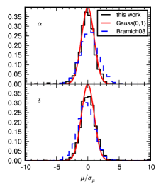
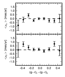
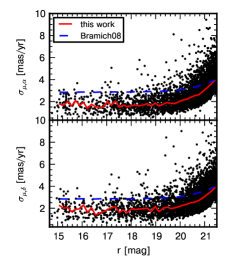
Figure 1.— Left panels: Normalized histogram of proper motions of spectroscopic QSOs measured relative to the photometric QSOs normalized by the error bar provided by the modeling. Red lines are Gaussians with zero mean and unity dispersion. Blue dashed curves show the histograms of the proper motions of spectroscopic QSOs from Bramich et al. (2008). Central panels: The median proper motion of spectroscopic QSOs relative to the photometric QSOs versus their color-difference. Right panels: The measured error bars on the the proper motions as a function of the $r$ band magnitude. The red lines show the median values of our measurement errors. The blue dashed lines show the median of proper motion errors from Bramich et al. (2008).

2.2. Systematic Errors in the Proper Motions

After performing the computation of the proper motion for individual stars, and before trying to measure the statistical proper motions for ensembles of stars, it is important to check for the presence of possible systematics, as well as to examine the accuracy of the error bars. Fig. 1 presents such an assessment. In this paper, we are focusing on the particular part of Stripe 82, which intersects with the Sgr stream. As systematic effects may depend on the right ascension, Fig. 1 uses only the proper motions in the right ascension range $20^{\circ}<\alpha<50^{\circ}$.

The left panel of Fig. 1 shows the histogram of proper motions of the spectroscopic QSOs measured relative to the photometric QSOs and normalized by the error bar provided by our fitting procedure. The red overplotted curve shows a Gaussian with the center at zero and unity dispersion. The excellent match of the histogram with the Gaussian curve shows that that the proper motions do not possess noticeable systematic offsets, and that the error bars on the proper motions are a faithful description of the precision. It is also quite clear from the plot that this is not true for proper motion measurements by Bramich et al. (2008), which have noticeable systematics and error underestimation. The middle panel of Fig. 1 shows the the proper motion of the spectroscopic QSOs relative to the photometric QSOs versus the $g\!-\!r$ color difference. The points with error bars show the median proper motion in bins of $g\!-\!r$, while the error bars are 1.48 times the median absolute deviation of proper motions within a corresponding $g\!-\!r$ bin. Since all the points lie within 1 $\sigma$ of zero, we conclude that the color-dependent terms in the proper motions are negligible down to the precision 0.1$-$0.2 mas yr^-1. This holds true at least within the color range $-0.2\lesssim g\!-\!r\lesssim 1$, which is the color-range applicable to 99% percent of the photometric QSOs. Later we will see that the proper motion of the Sgr stream determined from the photometric sample with $g\!-\!r\sim 0.3$, $g\!-\!i\sim 0.3$ and the spectroscopic sample with $g\!-\!r\sim 0.5$, $g\!-\!i\sim 0.75$ agree each other, further confirming the small level of color-related systematic errors. And last, the right panel of Fig. 1 shows the precision of our proper motion measurements as a function of $r$-band magnitude. There is a considerable scatter, but the median proper motion precision of $\sim 2$ mas yr^-1 is significantly better than that of Bramich et al. (2008) for large range of magnitudes.

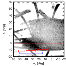
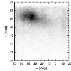
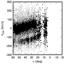
Figure 2.— Left panel: Density of MSTO stars ($0.25<g\!-\!i<0.35$, $19.8<r<22$) from SDSS DR8 in the southern Galactic hemisphere. The SDSS Stripe 82 region is delineated by the red line. Four horizontal error-bars show the range of right ascensions used to perform proper motion measurements in Stripe 82; red error-bars correspond to photometric samples, blue error-bars correspond to the spectroscopic sample. Center panel: The density of MSTO stars as a function of $r$ band magnitude and right ascension illustrating a distance gradient along the stream. Right panel Radial velocities of stars near the Stripe 82. These are SDSS measurements of stars with $\log($g$)<4$ and located near the Sgr orbit $-15\arcdeg<B<5\arcdeg$ and near Stripe 82 $|\delta|<20\arcdeg$. The Sgr stream is obvious at radial velocities of $-200$ km s${}^{-1}<V_{\rm GSR}<-100\,$km s^-1. The change of radial velocity along the stream is also quite prominent.

Table 1Radial velocities and dispersions of Sgr stars along the stream as traced by SDSS.

$\Lambda$	VGSR	$\sigma_{\rm V}$
deg	km s-1	km s-1
87.5	$-85.6\pm 2.1$	$13.7\pm 2.1$
92.5	$-100.5\pm 1.4$	$14.8\pm 1.5$
97.5	$-106.0\pm 1.5$	$11.1\pm 1.6$
102.5	$-121.0\pm 1.0$	$13.0\pm 1.0$
107.5	$-132.5\pm 1.2$	$13.8\pm 1.3$
112.5	$-140.5\pm 1.6$	$19.5\pm 1.4$
117.5	$-146.7\pm 1.5$	$16.7\pm 1.4$
125.0	$-154.7\pm 2.0$	$19.9\pm 2.8$
135.0	$-156.8\pm 2.8$	$27.2\pm 3.3$

3. The Sagittarius Stream

The Sgr stream in the southern Galactic hemisphere is known to have a complex structure. Koposov et al. (2012) used main-sequence turn-off (MSTO) stars extracted from SDSS Data Release 8 (DR8) to demonstrate the existence of two streams – a thicker, brighter stream and a thinner, fainter stream displaced by $\sim 10^{\circ}$. The brighter stream has multiple turn-offs as well as a prominent red clump, whereas the fainter stream does not. Koposov et al. (2012) argued that the brighter stream was composed of more than one stellar population, including some metal-rich stars, whereas the fainter stream is dominated by a single metal-poor population.

Here, we are primarily interested in the intersection of the Sgr stream with the SDSS Stripe 82. Fig. 2 shows the density of MSTO stars extracted via the cuts $0.25<g\!-\!i<0.35$ and $19.8<r<22.5$ in the southern hemisphere, together with Stripe 82 demarcated by the red lines. Again, two distinct streams structures are clearly visible – a brighter one crossing the Equator and Stripe 82 at a right ascension of $\sim 35^{\circ}$ and a dimmer one crossing the Equator at a right ascension of $\sim 15^{\circ}$. The magnitude distribution of MSTO stars along Stripe 82 is shown in the middle panel of Fig. 2. The Sgr streams are clearly evident, with the brighter stream visible at $\alpha\sim 35^{\circ}$ and fainter one at $\alpha\sim 15^{\circ}$. Since the distances to the streams are not constant with $\alpha$, and since Stripe 82 crosses the stream at an angle, we observe a clear distance gradient with right ascension.

The right panel of Fig. 2 shows the radial velocity as a function of right ascension for giant stars, extracted by the cut $\log(g)<4$ using the SDSS spectroscopic measurements. This time not only are stars within Stripe 82 included, but also those satisfying $|\delta|<20^{\circ}$ and lying near the stream ($-15\arcdeg<B<5\arcdeg$). As already found by Watkins et al. (2009), the Sgr stream is visible at the $V_{\rm GSR}\sim-150$ km s${}^{-1}\$. The figure also shows the variation of radial velocities as the stream stars return from the apocenter of the Sgr orbit. As they will be needed later, we extract the radial velocities along the stream, together with the velocity dispersion, by fitting a Gaussian to the Sgr signal. Although Figure 2 shows the radial velocities as a function of right ascension, it is important to realise that we perform these fits in bins along $\Lambda$, which is the angle along the stream from the remnant, measured positive in the trailing direction, as defined in Majewski et al. (2003)). The resulting measurements as a function of $\Lambda$ are shown in Table 1.

Importantly, Fig. 2 demonstrates that the Sgr stream stars are visible as a distinct bright feature in magnitude and velocity space. Therefore, this information can be used to select Sgr member stars and statistically measure their properties such as proper motion.

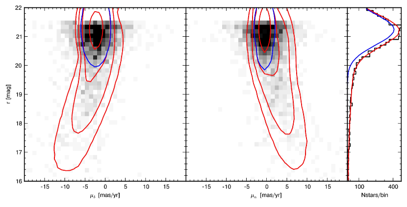
Figure 3.— The bright Sgr stream component at $25^{\circ}<\alpha<40^{\circ}$ Left and Middle panels: Greyscale shows the 2D distribution of proper motions and magnitudes, while the red contours show the total error-deconvolved Gaussian mixture model. The component of the model corresponding to the stream is shown in blue. Right panel: 1D projection onto the apparent magnitude axis of the left panel. The histogram of the data is shown in black, red curve shows the Gaussian mixture model of the luminosity function, whilst the model of the stream contribution is shown in blue.

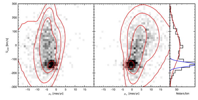
Figure 4.— Left and Middle panels: Greyscale shows 2D histograms of proper motions and the GSR radial velocities corrected for the stream’s radial velocity gradient for all stars with SDSS spectra and $\log(g)<$4 in Stripe 82. Red contours show the error-deconvolved Gaussian mixture model of the data. Right panel: The histogram of the radial velocities. The Gaussian mixture model of the radial velocities is shown by the red curve and the stream component in blue.

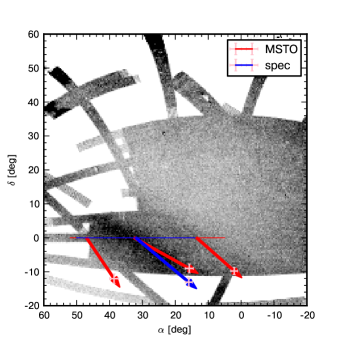
Figure 5.— Sgr streams in the South with the proper motion vectors overplotted. The red vectors indicate the measurements performed using the photometrically selected MSTO stars at three different locations along the Stripe. Blue vector is for the spectroscopic sample. The measured error-bars of proper motions are shown in pink. The proper motion vectors have been corrected for the solar motion, assuming the distances from Koposov et al. (2012) and $V_{LSR}=235$ km s^-1 and peculiar velocity from Coşkunoǧlu et al. (2011).

Table 2Proper motions measurements

Field	$\alpha_{1}$	$\alpha_{2}$	$\mu_{\alpha}\,cos(\delta)$	$\mu_{\delta}$	$\sigma_{\mu,\alpha\,cos(\delta)}$	$\sigma_{\mu,\delta}$	$\mu_{l}\,cos(b)$	$\mu_{b}$	$\sigma_{\mu,l}$	$\sigma_{\mu,b}$
	deg	deg	mas/yr	mas/yr	mas/yr	mas/yr	mas/yr	mas/yr	mas/yr	mas/yr
FP1	5.00	22.00	0.05	-2.51	0.11	0.11	0.10	-2.51	0.11	0.12
FP2	25.00	40.00	-0.50	-2.24	0.09	0.09	0.81	-2.15	0.09	0.11
FP3	42.00	52.00	0.19	-2.36	0.14	0.14	1.87	-1.45	0.11	0.15
FS4	14.00	50.00	-0.42	-2.65	0.11	0.13	1.07	-2.46	0.11	0.11

Note. — $\alpha_{1}$, $\alpha_{2}$ columns denote the edges of the boxes in right ascension in Stripe 82 used to perform the proper motion measurements

Table 3Positions and velocities of the Sgr stream.

Field	$\Lambda$	B	X	Y	Z	Distance	U	$\sigma_{U}$	V	$\sigma_{V}$	W	$\sigma_{W}$
	deg	deg	kpc	kpc	kpc	kpc	km s-1	km s-1	km s-1	km s-1	km s-1	km s-1
FP1	89.5	10.0	-15.0	9.6	-22.6	25.4	194	14	-46	14	23	8
FP2	106.1	0.6	-23.5	5.2	-24.4	29.1	290	12	33	14	-20	9
FP3	118.6	-6.7	-31.4	0.4	-25.0	33.9	270	17	-57	24	-48	16
FS4	105.6	0.8	-23.2	5.3	-24.3	28.9	308	15	-16	18	-40	11

Note. — $\Lambda$, B, X, Y, Z correspond to the centers of the fields where the proper motions are measured.

4. Modeling proper motions

As demonstrated above, in the Southern Galactic hemisphere, it is possible to achieve clean separation of the Sgr trailing tail stars and the Galactic foreground in both apparent magnitude and the radial velocity space. However, even for high-confidence stream members, the uncertainty of individual proper motion measurements ($\sim 2-3$ mas yr^-1; see Section 2) is comparable or higher than the expected tangential velocity of the stream ($\sim 1-3$ mas yr^-1; Law & Majewski, 2010a). It is therefore crucial to combine the signal from as many stream members as possible to beat down the noise. Koposov et al. (2010) have shown that, for the regions of apparent magnitude and radial velocity space dominated by the stream, an accurate measurement of the systemic proper motion of an ensemble of stars belonging to the stream can be obtained through simple background subtraction.

Alternatively, the overall stellar distribution in the space of observables can be modeled, yielding the direct contributions of the Galaxy and the stream. If such models can be cast in the 3D space of proper motion and magnitude or radial velocity, it is feasible that a superior measurement of the proper motion can be achieved as the contribution of the background to both systematic and random noise will be reduced. Unfortunately, adequate analytical models of the Sgr stream and the Galaxy are not readily available. Therefore, we choose to approximate these distributions by a sum of multi-dimensional Gaussians. This so-called Gaussian mixture is a well known semi-parametric technique widely used to model multi-dimensional datasets (McLachlan & Peel, 2000). Gaussian mixtures have several key properties that make the model-fitting straightforward and fast. First, the uncertainties associated with the measurements (as well as the missing data) are naturally incorporated into the model. Secondly, there exists a guaranteed fast convergence procedure – the Expectation Minimisation (EM) algorithm (Dempster et al., 1977). In this work, we have used the extreme-deconvolution package, the open-source Gaussian mixture implementation by Bovy et al. (2011).

4.1. Photometric sample

As evident from the dissection of the SDSS dataset shown in Fig. 2, main sequence turn-off stars (MSTO) are the most numerous Sgr stream specimens available to carry out the proper motion analysis. The typical density of the MSTO stars in the stream is 150 stars per square degree, compared to the foreground density of around 50. Stripe 82 slices through both the bright and the faint streams at an angle, resulting in a slightly tilted bi-modal distribution in the plane of right ascension and $r$ band magnitude. A faint Eastern wing to the bright Stream can also be discerned at higher right ascension (see middle panel of Fig. 2).

Motivated by the evolution of the distance and the structure of the stream along the Stripe, we split the MSTO sample into three parts: the faint stream at $5^{\circ}<\alpha<22^{\circ}$, the bright stream at $25^{\circ}<\alpha<40^{\circ}$, and the Eastern wing of the bright stream at $42^{\circ}<\alpha<52^{\circ}$ (we label those fields as FP1, FP2, FP3 respectively; they are shown by red error-bars on Fig. 2). In each of the three right ascension bins, the overall 3D distribution of MSTO stars in the space of ($\mu_{\alpha},\mu_{\delta},{\rm r}$) was modeled with a mixture of 5 Gaussians, The initial guess for the free parameters was obtained by running the K-means algorithm (MacQueen, 1967). The choice of number of Gaussians ($N_{\rm gau}$) was motivated by looking at the cross-validated log-likelihood (Arlot & Celisse, 2010) as a function of $N_{\rm gau}$. This initially rises as a function of $N_{\rm gau}$, peaks at $N_{\rm gau}\sim$ 5 and stays roughly constant for $N_{gau}>$5, demonstrating the goodness of fit and the absence of overfitting. We have also made sure that the objects in the Sgr stream are represented by a single Gaussian. When applying the extreme deconvolution, we force the covariance matrix for the Sgr component to be diagonal, e.g. assuming zero covariance between the proper motion and the apparent magnitude. The proper motions for the stream stars were not corrected for the solar reflex motion. The errors in the proper motion measurement, i.e. the uncertainties in determining the centre of the Gaussian representing the Sgr Stream, were determined either from bootstrap procedure or from the Hessian matrix of the likelihood function.

Fig. 3 shows the data analysed as well as the best fit Gaussian mixture model of the main Sgr stream $25^{\circ}<\alpha<40^{\circ}$. It is reassuring to see that the Gaussian mixture model was able to describe the data distribution adequately. The resulting measurements of the proper motion together with the uncertainties are given in Table 2. Among $\sim$ 7000 stars analyzed, according to the model, $\sim$ 4000 stars belong to Sgr, while $\sim$ 3000 stars belong to the background/foreground population.

4.2. Spectroscopic sample

The number of members of the Sgr stream with SDSS spectroscopic measurements is significantly smaller than the number of MSTO stars used in the previous section. Despite this, knowledge of the radial velocities and surface gravities allows us to have much purer samples of the Sgr stream members. In this section, we perform a complementary measurement of the stream’s proper motion using spectroscopic members only.

To this end, we select all stars with spectra in Stripe 82 lying at $14^{\circ}<\alpha<50^{\circ}$ ( we label this area FS4 and show it with the blue error-bar on Fig. 2) and classified by the SDSS spectroscopic pipeline as giants $\log(g)<4$. Despite very wide range of selected right ascensions, most of the Sgr members with spectroscopy in the Stripe 82 region located at the center of the bright stream, at $\alpha\sim 30\arcdeg$. According to the right panel of Fig. 2, the Sgr stream’s radial velocity changes along the Stripe. Therefore, to ease the modeling, we subtract the variation of the radial velocity centroid from the data using the measurements presented in Table 1. The resulting radial velocity is approximately constant as a function of RA, and the measurements of proper motions and radial velocities $\mu_{\alpha},\mu_{\delta},\tilde{V}_{\rm GSR}=V_{\rm GSR}-V_{\rm model,GSR}(\Lambda)$ can now be represented by a mixture of Gaussians.

We run the extreme deconvolution on the sample of $\sim$1500 stars and find that 3 Gaussian components are sufficient to describe the dataset. We follow the strategy outlined in Section  4.1, with the difference that the covariance matrix of the Gaussian representing the stream component is now set free. Fig. 4 shows the density distribution of the data, together with the best-fit Gaussian mixture model for the Stripe 82 stars with spectra. By comparing the grey-scale density with the red contours, we can confirm that the model has captured the properties of the dataset reasonably well. The last line of Table 2 reports the values of the proper motion for the spectroscopic sample, and confirms that the measurements for the two independent stream samples agree within 2$\sigma$. It is also particularly reassuring since Sgr members in the spectroscopic sample have very different colors (g$-$i $\sim$ 0.75) from the Sgr members in the photometric sample (g$-$i $\sim$ 0.3) of the Sgr giants. Therefore the agreement of the proper motions from two samples is a proof of a small level of color-related systematic effects.

The proper motion signals we have measured have a very large contribution of the solar reflex motion. Since we have distance estimates to the Sgr stream in the South measured elsewhere (e.g. Koposov et al., 2012), we can correct for this and check whether the proper motions are actually aligned with the streams. Figure 5 shows the proper motion vectors after applying the solar reflex corrections. As we can clearly see, the proper motions are indeed properly aligned with the streams and are consistent with each other. For this calculation we have still used the distance to the faint stream as given by Koposov et al. (2012, 2013), although, there is evidence in Slater et al. (2013) that the stream the faint stream is 3$-$5 kpc closer.

5. Comparisons to earlier work

There are many models of the Sgr stream in the literature, all purporting to provide the distances, velocities and proper motions as a function of position on the sky (e.g. Fellhauer et al., 2006; Peñarrubia et al., 2010; Law & Majewski, 2010a). Although quite detailed, all the models fail to reproduce at least some of the features that we see on the sky (e.g., Niederste-Ostholt et al., 2010; Koposov et al., 2012). But, it still instructive to see where our data measurements lie relative to the existing models. We have chosen the Law & Majewski (2010a) model as a comparison benchmark, because it is arguably the most comprehensive and up-to-date.

There are several caveats to be borne in mind. The first is related to the fact that while our central measurement in Stripe 82 at $\alpha\sim 35\arcdeg$ or $(\Lambda,B)\sim(100\arcdeg,0\arcdeg)$ corresponds directly to the center of the trailing tail in the simulation, the fainter stream which crosses Stripe 82 at $\alpha\sim 15\arcdeg$ or $\Lambda,B\sim(90\arcdeg,10\arcdeg)$ doesn’t have a counterpart in the simulation by Law & Majewski (2010a). The second is related to the choice of rotation velocity of the Local Standard of Rest. As shown in Carlin et al. (2012), the observed proper motion signal is sensitive to the adopted V_LSR. The models of Law & Majewski (2010a) have been computed and fitted under the assumption of the IAU standard value of the $V_{\rm LSR}$=220 km s^-1, while the current best estimates are slightly higher at $230-250$ km s^-1(Bovy et al., 2009; Reid et al., 2009; Deason et al., 2011). Throughout the paper, we adopted the value of 235 km s^-1.

Fig. 6 shows our data points overplotted onto the distribution of tracers from Law & Majewski (2010a) model, where we have selected tracers from the trailing tail only ($Lmflag=-1$ and $Pcol<=7$), and lying within 20 degrees of Stripe 82 ($|\delta|<20$). The $\Lambda$ values of our measurements correspond to the centers of the rectangular areas used to perform the measurements, and the error-bars indicate the extent of those areas. The agreement for the central field ($\Lambda\sim 105\arcdeg$), as well as for the edge of the bright stream ($\Lambda\sim 120\arcdeg$), is quite good. At the location of the fainter Sgr stream (empty circle on the plot), the model doesn’t have many particles, as expected. In order to facilitate further comparisons, Table 3 gives the positions and velocities corresponding to our measurements. Here, ($X,Y,Z$) and ($U,V,W$) are in a right handed Galactocentric coordinate system with the Sun located at $X=-$8.5 kpc, and $V_{\rm LSR}=235$ km s^-1. The distances taken from the work by Koposov et al. (2012), and the error on the velocities does not take into account any possible systematic error distance of $\sim 10\%$. Readers wishing to compare Sgr disruption models with our observations should use Table 3 only for rough checks. A proper comparison entails measuring the average proper motions within the same area of the sky as we do and comparing these numbers directly with our Table 2.

We also compare our measurements with the data from Carlin et al. (2012). Out of 6 fields analysed by Carlin et al. (2012), 4 have measurable Sgr signal and only 2 of those (SA 93 and SA 94) lie near the Stripe 82. The other 2 fields with detectable Sgr signal are $\sim$ 15 degrees away from the Stripe 82. As Figure 6 shows, the error-bars of our measurements are much tighter than Carlin et al. (2012), and the proper motions themselves agree approximately within the combined errors.

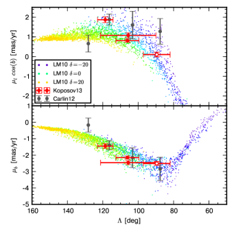
Figure 6.— The comparison of the measured Stripe 82 proper motions (red with error bars) with both the earlier measurements of Carlin et al. (2012, grey with error bars) and the simulations of Law & Majewski (2010a, blue,green,yellow dots). Our measurement of the proper motion of the fainter of the two trailing tails is identified by an empty red circle. Note that the datapoints from Law & Majewski (2010a) are selected from trailing tail only and from the region near Stripe 82 $|\delta|<20\arcdeg$. The points are colored according to $\delta$ such that points with $\delta\sim-20\arcdeg$ are dark blue, points with $\delta\sim 20\arcdeg$ are orange, and points near Stripe 82 are light-green. Two of the fields from Carlin et al. (2012) lie within Stripe 82, while two other fields are $\sim$ 15 degrees away from the Stripe 82.

6. Conclusions

We have measured the proper motion of the Sgr stream using Stripe 82 data. By tying the astrometry to the known QSOs and combining the measurements for large samples of stars, we have been able to achieve high precision proper motions. Our measurements have been performed for two distinct groups – spectroscopically selected red giants/subgiants with SDSS radial velocities and photometrically selected MSTO stars. The proper motions of those agree very well and after correcting for the solar reflex motion are tightly aligned with the Sgr stream. Our results are in agreement with earlier measurements by Carlin et al. (2012), but, by virtue of the large numbers of stars in our samples, our statistical error bars are substantially smaller, typically about $0.1$ mas yr^-1.

There are three fields in Stripe 82 for which the proper motion of the photometric sample has been measured, and one field for the spectroscopic sample. Combining this information with distances from Koposov et al. (2012) gives us the full six dimensional phase space coordinates of the Sgr trailing stream at four locations along Stripe 82. We provide a table of three dimensional positions and velocities of Sgr stream stars, in which the contributions of the motion of the Sun and LSR have been removed.

To complement the work on the Sgr streams in the South, it would be particularly useful to carry out a corresponding kinematical analysis for the streams in the North. This is a subject to which we plan to return in a later contribution. The combination of the proper motions, radial velocities and distances in both Galactic hemispheres should allow us to make further progress in the understanding of the complicated structure of the Sgr streams and solve some of the riddles posed by their existence.

References

- Abazajian et al. (2009) Abazajian, K. N., Adelman-McCarthy, J. K., Agüeros, M. A., et al. 2009, ApJS, 182, 543
- Annis et al. (2011) Annis, J., Soares-Santos, M., Strauss, M. A., et al. 2011, arXiv:1111.6619
- Arlot & Celisse (2010) Arlot, S., & Celisse, A. 2010, Stat. Surv., 4, 40
- Becker et al. (2008) Becker, A. C., Agol, E., Silvestri, N. M., et al. 2008, MNRAS, 386, 416
- Belokurov et al. (2006) Belokurov, V., Zucker, D. B., Evans, N. W., et al. 2006, ApJ, 642, L137
- Bovy et al. (2009) Bovy, J., Hogg, D. W., & Rix, H.-W. 2009, ApJ, 704, 1704
- Bovy et al. (2011) Bovy, J., Hogg D. W., & Roweis, S. T. 2011, Ann. Appl. Stat. 5, 2B, 1657
- Bramich et al. (2008) Bramich, D. M., Vidrih, S., Wyrzykowski, L., et al. 2008, MNRAS, 386, 887
- Carlin et al. (2012) Carlin, J. L., Majewski, S. R., Casetti-Dinescu, D. I., et al. 2012, ApJ, 744, 25
- Chou et al. (2007) Chou, M.-Y., Majewski, S. R., Cunha, K., et al. 2007, ApJ, 670, 346
- Chou et al. (2010) Chou, M.-Y., Cunha, K., Majewski, S. R., et al. 2010, ApJ, 708, 1290
- Coşkunoǧlu et al. (2011) Coşkunoǧlu, B., Ak, S., Bilir, S., et al. 2011, MNRAS, 412, 1237
- Deason et al. (2011) Deason, A. J., Belokurov, V., & Evans, N. W. 2011, MNRAS, 411, 1480
- Dempster et al. (1977) Dempster A.P., Laird N.M & Rubin, D.B. Journal of the Royal Statistical Society. Series B (Methodological), 1977, 39, 1
- Fellhauer et al. (2006) Fellhauer, M., Belokurov, V., Evans, N. W., et al. 2006, ApJ, 651, 167
- Helmi (2004) Helmi, A. 2004, MNRAS, 351, 643
- Johnston et al. (2005) Johnston, K. V., Law, D. R., & Majewski, S. R. 2005, ApJ, 619, 800
- Koposov & Bartunov (2006) Koposov, S., & Bartunov, O. 2006, Astronomical Data Analysis Software and Systems XV, 351, 735
- Koposov et al. (2010) Koposov, S. E., Rix, H.-W., & Hogg, D. W. 2010, ApJ, 712, 260
- Koposov et al. (2012) Koposov, S. E., Belokurov, V., Evans, N. W., et al. 2012, ApJ, 750, 80
- Koposov et al. (2013) Koposov, S. E., Belokurov, V., Evans, N. W., 2013 (Erratum on ApJ 750, 80)
- Kowalski et al. (2009) Kowalski, A. F., Hawley, S. L., Hilton, E. J., et al. 2009, AJ, 138, 633
- Kuijken & Tremaine (1994) Kuijken, K., & Tremaine, S. 1994, ApJ, 421, 178
- Law et al. (2005) Law, D. R., Johnston, K. V., & Majewski, S. R. 2005, ApJ, 619, 807
- Law & Majewski (2010a) Law, D. R., & Majewski, S. R. 2010a, ApJ, 714, 229
- Law & Majewski (2010b) Law, D. R., & Majewski, S. R. 2010b, ApJ, 718, 1128
- MacQueen (1967) MacQueen, J. 1967, Some methods for classification and analysis of multivariate observations., Proc. 5th Berkeley Symp. Math. Stat. Probab., Univ. Calif. 1965/66, 1, 281-297 (1967).
- Majewski et al. (2003) Majewski, S. R., Skrutskie, M. F., Weinberg, M. D., & Ostheimer, J. C. 2003, ApJ, 599, 1082
- Majewski et al. (2004) Majewski, S. R., Kunkel, W. E., Law, D. R., et al. 2004, AJ, 128, 245
- Monaco et al. (2007) Monaco, L., Bellazzini, M., Bonifacio, P., et al. 2007, A&A, 464, 201
- O’Mullane et al. (2005) O’Mullane, W., Li, N., Nieto-Santisteban, M., et al. 2005, arXiv:cs/0502072
- Niederste-Ostholt et al. (2010) Niederste-Ostholt, M., Belokurov, V., Evans, N. W., & Peñarrubia, J. 2010, ApJ, 712, 516
- Niederste-Ostholt et al. (2012) Niederste-Ostholt, M., Belokurov, V., & Evans, N. W. 2012, MNRAS, 422, 207
- McLachlan & Peel (2000) McLachlan, G., & Peel, D. Finite Mixture Models. Wiley series in Applied Probability and Statistics, Wiley, 2000.
- Peñarrubia et al. (2010) Peñarrubia, J., Belokurov, V., Evans, N. W., et al. 2010, MNRAS, 408, L26
- Pedregosa et al (2011) F. Pedregosa, G. Varoquaux, A. Gramfort, et al. 2011, Journal of Machine Learning Research, 12, 2825
- Reid et al. (2009) Reid, M. J., Menten, K. M., Zheng, X. W., et al. 2009, ApJ, 700, 137
- Richards et al. (2009) Richards, G. T., Myers, A. D., Gray, A. G., et al. 2009, ApJS, 180, 67
- Sesar et al. (2007) Sesar, B., Ivezić, Ž., Lupton, R. H., et al. 2007, AJ, 134, 2236
- Schneider et al. (2010) Schneider, D. P., Richards, G. T., Hall, P. B., et al. 2010, AJ, 139, 2360
- Slater et al. (2013) Slater, C. T., Bell, E. F., Schlafly, E. F., et al. 2013, ApJ, 762, 6
- Smith et al. (2009a) Smith, M. C., Evans, N. W., Belokurov, V., et al. 2009a, MNRAS, 399, 1223
- Smith et al. (2009b) Smith, M. C., Evans, N. W., & An, J. H. 2009b, ApJ, 698, 1110
- Smith et al. (2012) Smith, M. C., Whiteoak, S. H., & Evans, N. W. 2012, ApJ, 746, 181
- Vidrih et al. (2007) Vidrih, S., Bramich, D. M., Hewett, P. C., et al. 2007, MNRAS, 382, 515
- Watkins et al. (2009) Watkins, L. L., Evans, N. W., Belokurov, V., et al. 2009, MNRAS, 398, 1757