Precession of the Sagittarius stream

Abstract

Using a variety of stellar tracers – blue horizontal branch stars, main-sequence turn-off stars and red giants – we follow the path of the Sagittarius (Sgr) stream across the sky in Sloan Digital Sky Survey data. Our study presents new Sgr debris detections, accurate distances and line-of-sight velocities that together help to shed new light on the puzzle of the Sgr tails. For both the leading and the trailing tail, we trace the points of their maximal extent, or apo-centric distances, and find that they lie at $R^{\rm L}=47.8\pm 0.5$ kpc and $R^{\rm T}=102.5\pm 2.5$ kpc respectively. The angular difference between the apo-centres is $93\aas@@fstack{\circ}2\pm 3\aas@@fstack{\circ}5$, which is smaller than predicted for logarithmic haloes. Such differential orbital precession can be made consistent with models of the Milky Way in which the dark matter density falls more quickly with radius. However, currently, no existing Sgr disruption simulation can explain the entirety of the observational data. Based on its position and radial velocity, we show that the unusually large globular cluster NGC 2419 can be associated with the Sgr trailing stream. We measure the precession of the orbital plane of the Sgr debris in the Milky Way potential and show that, surprisingly, Sgr debris in the primary (brighter) tails evolves differently to the secondary (fainter) tails, both in the North and the South.

1 Introduction

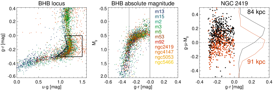
Figure 1: BHB stars in SDSS bands. Left: BHB $u-g,g-r$ locus as traced by the BHB stars in the Galactic star clusters. Each dot represents a BHB candidate star coloured according to the membership in one of the 11 clusters listed in the middle panel. The polygon shows the region proposed byg Yanny et al. (2000) to select BHBs. Middle: BHB absolute magnitude as a function of $g-r$ colour. Note how stars belonging to different star clusters group densely around similar intrinsic luminosity which changes slowly with $g-r$ colour. Vertical black lines mark the boundaries of the selection region shown in the Left panel. Right: Offset between the distance modulus calculated using eq. 7 of Deason et al. (2011) and the distance modulus suggested by Harris (1996) for the BHB candidate stars in the globular cluster NGC 2419. Red dots are for the assumed heliocentric distance to NGC 2419 of 91 kpc. Curves show the histograms of the distance modulus offset.

As long as Newton’s law of attraction holds true, an orbit gives the most straightforward method of inferring the underling gravitational potential. Such an inference is truly unambiguous when the orbit mapped is nearly complete, as demonstrated beautifully by the recent measurements of the mass of the Milky Way’s central black hole (e.g. Ghez et al. 2008). At larger Galactocentric distances, orbital periods quickly grow to a significant fraction of the Hubble time, rendering the tracking of a trajectory impractical. Yet, it is still possible to establish the paths of some infalling Galactic fragments rather accurately even at distances beyond many tens of kpc. Certain Milky Way satellites sprout stellar tidal tails long enough to delineate some of their orbit. These include the Sagittarius dSph stream (Majewski et al., 2003), the tails of the Palomar 5 globular cluster (Odenkirchen et al., 2003), as well as the Orphan (Belokurov et al., 2007) and the GD-1 (Grillmair & Dionatos, 2006) streams.

So far, the most robust inference of the Galactic potential based on the measurements of a stellar stream has been the one carried out with the GD-1 system by Koposov et al. (2010). Even though only $\sim 100^{\circ}$ of arc of the stream has been mapped, the detailed phase-space information and the intrinsic coldness of the stellar debris allowed the authors to avoid the degeneracies inherent in the stream modelling process (e.g. Eyre & Binney 2009). However, given the orbit of the GD-1 stream, the circular velocity measurement it facilitates, while independent and robust, is limited to the range of galactocentric distances accessible to other techniques (e.g. Bovy et al. 2012).

To reach into the outer Galactic halo, more distant and luminous streams like the Orphan or Sagittarius are needed. The kinematically cold Orphan stream seems to possess the properties ideal for orbit inference. However, compared to the total of only $\sim 60^{\circ}$ of the available detections of the Orphan Stream at distances between 30 and 50 kpc, there exists much more abundant information for both the leading and the trailing tail of the Sgr stream. Each extends some $\sim 180^{\circ}$ of arc, probing Galactocentric distances in the range of 20-100 kpc. As of today, the narrow, but relatively faint Orphan stream remains largely unstudied, yet a broad-brush picture of the wide and luminous Sgr stream is slowly taking shape, thanks to the diversity of the disruption models at hand (e.g. Ibata et al. 2001; Helmi 2004; Johnston et al. 2005; Fellhauer et al. 2006; Law & Majewski 2010; Peñarrubia et al. 2010).

The most comprehensive model to date (Law & Majewski, 2010) fits accurately the 3D positions and the radial velocities of the brightest components of the leading and the trailing tail as mapped by Belokurov et al. (2006); Law et al. (2004), and Majewski et al. (2003, 2004) respectively. This N-body simulation, however, does not provide an explanation for the tail “bifurcations” observed both in the North and the South (Belokurov et al., 2006; Koposov et al., 2012). Furthermore, the model does not produce Sgr tidal debris running with the opposite distance gradient at the locations of the leading tail around the North Galactic Cap (Branch C in the notation of Fellhauer et al. (2006) as measured in Belokurov et al. (2006)), or the distant the debris as detected by Newberg et al. (2003) and recently confirmed by Ruhland et al. (2011) in the direction of the Galactic anti-centre. Naturally, given the wealth of the data available for the Sgr system and the inherent complexity of the Milky Way’s gravitational potential, it is prudent to adopt the modelling strategy in which some of the many unknowns are fixed at their best-guess values. For their experiment, Law & Majewski (2010) chose to fix most of the orbital properties of the Sgr progenitor, as well as many of the ingredients describing the Galactic potential. For example, the potential of the dark matter halo is set to be logarithmic, while the importance of changing the shape of the dark halo is explored.

In this Paper, based on the Sloan Digital Sky Survey Data Release 8 (SDSS DR8) we i) present several new detections of the Sgr debris in the Galactic North, ii) refine some of the stream distances and iii) substantiate the 3D data with the measurements of the stream’s radial velocity. As a result, we show that the Branch C (Belokurov et al., 2006; Fellhauer et al., 2006) and the anti-centre debris (Newberg et al., 2003; Ruhland et al., 2011) are all part of the very long trailing tail of the Sagittarius dwarf. We show that at the very edges of the SDSS footprint, both the leading and trailing tail reach their respective apo-centres, thus indicating that the galactocentric orbital precession (or apsidal precession) of the Sgr dSph is close to $\sim 95^{\circ}$. This is to be compared with logarithmic haloes, where the orbital precession is typically $\sim 120^{\circ}$. The lower rate of the orbital precession signifies a sharper drop in the dark matter density as a function of Galactocentric radius. We also measure the precession of the plane of the Sgr debris. This is related to the Sgr orbital plane evolution under the torques from the disk and the dark halo of the Milky Way.

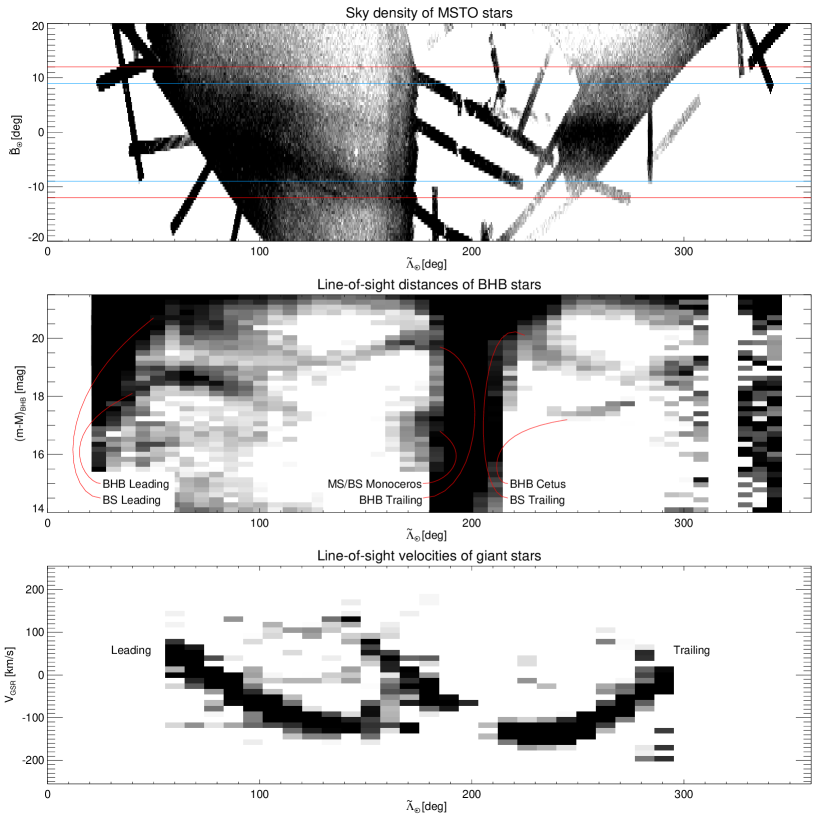
Figure 2: Sagittarius stream tomography with multiple tracers. Darker regions correspond to enhanced stellar density. Top: Sky density of MSTO stars in the Sgr stream coordinate system similar to that defined by Majewski et al. (2003). Red (blue) lines show the range of latitude $B$ used to select stars for Middle (Bottom) panel. Middle: Density of stream stars in the plane of Sgr stream longitude $\tilde{\Lambda}_{\odot}$ and distance modulus. For this plot, BHB candidate stars with $-12^{\circ}<\tilde{B}_{\odot}<12^{\circ}$ are selected using the criteria of Yanny et al. (2000), while the distances are assigned according to eq. 7 of Deason et al. (2011). In the North, the Sgr leading tail is clearly seen at $40^{\circ}<\tilde{\Lambda}_{\odot}<120^{\circ}$ in both BHBs ($17<m-M<19$) and BSs ($19<m-M<21.5$). Note also the unambiguous detection of the trailing debris at $130^{\circ}<\tilde{\Lambda}_{\odot}<190^{\circ}$. In the South, the Sgr trailing debris can be traced with BS stars in the range $220^{\circ}<\tilde{\Lambda}_{\odot}<290^{\circ}$. Bottom: Density of the stream stars in the plane of $\tilde{\Lambda}_{\odot}$ and the line-of-sight velocity $V_{\rm GSR}$. For this plot, giant stars with $-9^{\circ}<\tilde{B}_{\odot}<9^{\circ}$ are selected using the criteria in eq. 1 from the SDSS spectroscopic database. Note, that the tentative trailing velocity signal at $140^{\circ}<\tilde{\Lambda}_{\odot}<190^{\circ}$ appears to be the natural continuation of the radial velocity run in the South, only interrupted by the disk at $190^{\circ}<\tilde{\Lambda}_{\odot}<210^{\circ}$

2 Stream tomography with multiple tracers

For all the subsequent analysis, we correct the SDSS photometry for the effects of extinction using the dust maps of Schlegel et al. (1998). To correct for the solar reflex motion, we adopt $V_{\rm LSR}=235$ km/s and $(U,V,W)=(11.1,12.2,7.25)$ (Schönrich et al., 2010).

2.1 Blue Horizontal Branch stars in SDSS and the distance to NGC 2419

To measure mean heliocentric distances to portions of the Sgr stream within the SDSS field of view, we use Blue Horizontal Branch (BHB) stars. The luminosity of BHBs does not vary to any significant degree with changing age and metallicity and is primarily a function of the star’s temperature, which makes them attractive standard candles. Yanny et al. (2000) have shown that by using the SDSS $u-g$ and $g-r$ colours, highly complete (for a particular range of effective temperatures) samples of BHBs can be selected with low levels of contamination. At high Galactic latitudes, the principal source of false positives within the boundaries of the colour-colour box proposed by Yanny et al. (2000) are the intrinsically less luminous Blue Straggler (BS) stars. Note that the photometrically-selected BHB sample analysed below has a non-zero BS contamination. This, however, does not affect the results as we do not study individual A-coloured stars, but instead measure the properties of stellar over-densities.

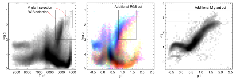
Figure 3: Selection of RGB and M giant stars from the SDSS spectroscopic sample. Left: Density of stars with spectra in the SDSS DR8 in the plane of effective temperature $T_{eff}$ and surface gravity $\log g$. Darker shades of grey mean higher density of stars. This is an analog of the familiar Hertzsprung-Russell diagram with the main sequence, the red giant branch and the blue horizontal branch all clearly visible. Solid lines give the boundaries used to select RGB and M giant candidate members of the stream. Middle: Density of stars in color $g-i$ and surface gravity $\log g$ plane, color-coded according to metallicity $[Fe/H]$. Red, Green and Blue channels of the image are constructed with grey-scale density distributions of stars in the three metallicity bins: $-0.75<[Fe/H]<0$, $-1.5<[Fe/H]<-0.75$ and $-3<[Fe/H]<-1.5$. The additional $g-i$ cut preferentially selects more metal-rich RGB stars. Right: Density of the SDSS DR8 stars with spectra in the color-color plane of $g-i,u-g$. The brighter and/or the more metal-rich M giants stand out clearly thanks to their redder $u-g$ color. With this in mind, an additional $u-g$ cut is used to produce a cleaner selection of the Sgr M giant candidates.

Figure 1 shows the properties of the candidate BHB stars in 11 Galactic star clusters analysed by An et al. (2008). The left panel of the Figure confirms the effectiveness of the colour cuts suggested by Yanny et al. (2000). BHBs from clusters with different stellar populations essentially lie on top of each other forming a tight locus going bluewards in $g-r$ at constant $u-g$ and eventually turning blue in $u-g$ at around $g-r\sim-0.35$. As is obvious from the middle panel of this Figure, the absolute magnitude of a BHB varies with its $g-r$ color, as governed by changing temperature. At small negative values of $g-r$, $M_{g}\sim 0.5$. However, on moving bluewards, the Horizontal Branch tips and by $g-r=-0.35$, the absolute magnitude is at least half a magnitude fainter. The behaviour of the centroid of the distribution of the Galactic globular cluster BHBs in the plane of absolute magnitude and $g-r$ colour can be described accurately with a 4th degree polynomial, as proposed by Deason et al. (2011). In what follows, we use Equation 7 from Deason et al. (2011) to assign distances to candidate BHB stars within the colour-colour box outlined in the Left panel of Figure 1.

Only one globular cluster has significant non-zero residuals when the distance modulus $(m-M)_{g}$ calculated using the BHB distance calibration described above is compared with $(m-M)_{g}$ found in the literature. This is illustrated in the right panel of Figure 1. As apparent from the histograms of the $(m-M)_{g}$ residuals in the right hand side of the panel, the distance modulus for NGC 2419 needs to be revised $\sim 0.2$ mag upwards, thus making its heliocentric distance not 84 kpc (Harris, 1996), but 91 kpc. Recently, Fermani & Schönrich (2013) presented new calibration of the BHB absolute magnitude based on theoretical isochrones. Compared to Deason et al. (2011) these models predict slightly higher ($\sim 0.1$ mag) luminosity for stars as metal-poor as those in NGC 2419. To test whether some of the 0.2 mag discrepancy observed here could be explained away by this effect, we checked the $(m-M)_{g}$ residuals for three more star clusters with $[{\rm Fe}/{\rm H}]<-2$, namely M 92, M15 and NGC 5053. The residuals for the stars in all three clusters stay firmly on zero. While our slightly higher distance estimate is mildly inconsistent with the value provided by Harris (1996), we are in agreement with the most recent RR Lyrae measurement by Di Criscienzo et al. (2011).

2.2 The Sgr Stream signal in the SDSS data

Majewski et al. (2003) and Koposov et al. (2010) have shown that measuring the properties of a stellar stream can be highly robust (even with small numbers of stream members) if the debris mapping is performed in a coordinate system aligned with the stream. We follow the prescription of Majewski et al. (2003) and transform equatorial RA and Dec into a heliocentric $\tilde{\Lambda}_{\odot},\tilde{B}_{\odot}$ coordinate system whose equator is aligned with the Sgr trailing tail. Note, however, that in this paper $\tilde{\Lambda}_{\odot}$ increases in the direction of Sgr motion, i.e. opposite to the convention used by Majewski et al. (2003). Likewise, the latitude axis $\tilde{B}_{\odot}$ points to the Galactic North pole instead of the South pole. This means that the coordinates given here can be transformed to those in Majewski et al. (2003) convention using the following simple equations: $\Lambda_{\odot}=360^{\circ}-\tilde{\Lambda}_{\odot}$ and $B_{\odot}=-\tilde{B}_{\odot}$. While this is a minuscule departure from the previously used notation, it seems more logical to point the principal axis of the stream coordinate system in the direction of the stream’s motion.

The top panel of Figure 2 shows the density of (primarily) MSTO stars selected using the colour-magnitude cuts identical to those in Koposov et al. (2012). Both “branches” of the Sgr leading tail are visible superposed onto the Virgo overdensity at $70^{\circ}<\tilde{\Lambda}_{\odot}<120^{\circ}$. Also visible are the Orphan stream at $130^{\circ}<\tilde{\Lambda}_{\odot}<150^{\circ}$ and the Monoceros ring at $\tilde{\Lambda}_{\odot}\sim 170^{\circ}$. The only tentative evidence of the presence of the trailing tail in the Northern SDSS data is the faint overdensity running between the Branches A and B at $150^{\circ}<\tilde{\Lambda}_{\odot}<160^{\circ}$ at constant $\tilde{B}_{\odot}\sim-5^{\circ}$. Note that even though the contiguous coverage of the main SDSS footprint runs out at $\tilde{\Lambda}_{\odot}\sim 70^{\circ}$ and $\tilde{\Lambda}_{\odot}\sim 170^{\circ}$, within $|\tilde{B}_{\odot}|<10^{\circ}$ there exist several stripes reaching as far out as $\tilde{\Lambda}_{\odot}\sim 40^{\circ}$ and $\tilde{\Lambda}_{\odot}\sim 190^{\circ}$, providing an additional $\sim 50^{\circ}$ along the stream.

Indeed, the stream is clearly visible at both lower and higher $\tilde{\Lambda}_{\odot}$, as revealed by the density of the candidate BHB stars in the middle panel of the Figure. Only the stars that lie inside the $u-g,g-r$ boundary shown in the Left panel of Figure 1 (see Yanny et al. 2000) and within $-12^{\circ}<\tilde{B}_{\odot}<12^{\circ}$ are included in this picture. The leading tail can be traced from $\tilde{\Lambda}_{\odot}\sim 35^{\circ}$ to $\tilde{\Lambda}_{\odot}\sim 120^{\circ}$ with both BHB at $17<(m-M)_{g}<19$ and BS stars at $(m-M)_{g}>19.5$. The stream signal traced by the A-coloured stars dries up much faster than that traced by the MSTO stars; this is simply the consequence of the declining stream luminosity and the decreasing distance as explained in Niederste-Ostholt et al. (2010).

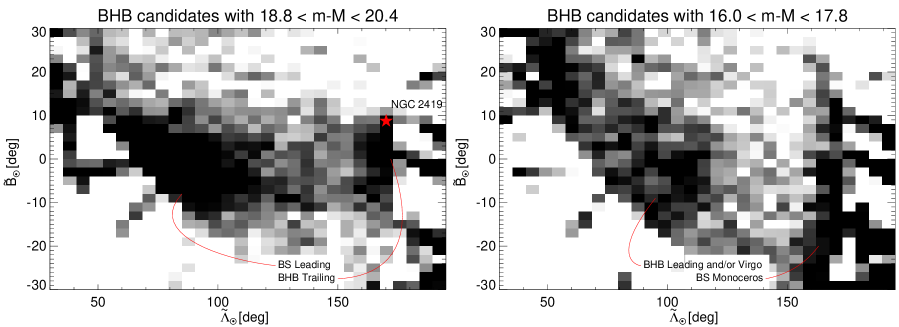
Figure 4: Sky density of the BHB candidates. Left: Stars with $18.8<m-M<20.4$ (see Middle panel of Figure 2). Both leading tail and trailing tail can be easily discerned. Globular cluster NGC 2419 appears projected right at the edge of the trailing stream. Right: Density of the brighter BHB candidate stars. None of the Sgr tails appears distinctly visible in this picture, although an over-density is detected at $80^{\circ}<\tilde{\Lambda}_{\odot}<120^{\circ}$, which could plausibly be attributed either to the portion of the Sgr leading stream falling into this distance range, or to the Virgo Stellar Structure. At high $\tilde{\Lambda}_{\odot}$, a narrow vertical band parallel to the Galactic disk is visible. The A-colored stars in this structure could either be young stars in the disk,alternatively they could be the denizens of the Monoceros stream.

The trailing tail is expected to enter the SDSS footprint at high $\tilde{\Lambda}_{\odot}$. In the middle panel of Figure 2, there are two density enhancements at $\tilde{\Lambda}_{\odot}>150^{\circ}$: a broad faint cloud at $16<(m-M)_{g}<17.5$ and a narrow sequence at $19<(m-M)_{g}<20.5$. To establish which of the two signals is contributed by the Sgr debris, the 2D histograms of the candidate BHB stars in the corresponding $(m-M)_{g}$ ranges are plotted in Figure 4. Dominating the Left panel of Figure 4 are two overdensities each ending sharply at $|\tilde{B}_{\odot}|>10^{\circ}$. The one at lower $\tilde{\Lambda}_{\odot}$ obviously corresponds to the Sgr leading tail, while the short stubby piece of the stream at higher $\tilde{\Lambda}_{\odot}$ clearly has not precessed as much as the nearby end of the Branch A (see top panel of Figure 2). The fact that the width of the distribution of the distant BHB stars matches that of the rest of the Sgr stream has already been noted by (Newberg et al., 2003). This picture is distinctly different from the one seen in the Right panel of the Figure, where the shape of the distribution of the brighter BHB-like stars bears little resemblance to the Sgr stream. At around $\tilde{\Lambda}_{\odot}\sim 110^{\circ}$, there appears an over-density that could correspond to either the brightest of the leading tail BHBs or stars in the Virgo over-density. Most importantly, at $\tilde{\Lambda}_{\odot}>160^{\circ}$, the stars are distributed in a band perpendicular to the direction of the stream, thus ruling out any connection to Sagittarius.

It is reasonable to conjecture that the debris traced by the distant BHB stars is contributed by the Sgr trailing tail that passed through the Galactic disk and is near its apo-centre at $\tilde{\Lambda}_{\odot}\sim 170^{\circ}$. To further test this hypothesis, the line-of-sight (LOS) velocities $V_{\rm GSR}$ of all SDSS DR8 giant stars in the vicinity of the equator of the Sgr coordinate system are plotted in the lower panel of Figure 2. The following magnitude, colour, effective temperature and surface gravity cuts are applied to pick out the giants:

$$\begin{split}17<g<21.5\\ 0.8<g-i<1.7\\ T_{eff}<5,500K\\ 1<\mathrm{log}(g)<3\end{split}$$ (1)

The first (apparent magnitude) cut is highly effective at eliminating the disk contamination by simply excising the brightest of the stars from the sample. The rationale for the remaining 3 selection criteria is illustrated in Figure 3. As obvious from the Figure, the effective temperature and the surface gravity cuts simply isolate the region dominated by the RGB stars. As the Sgr is somewhat more metal-rich as compared to the rest of the stellar halo, the additional $g-i$ is used to get rid of the bluer, more metal-poor RGBs. We argue that while this cut reduces the stream signal somewhat (as it is known that the Sgr tails contain a modest metal-poor population), it suppresses the halo contamination even more.

Within $-9^{\circ}<\tilde{B}_{\odot}<9^{\circ}$, the distribution of the stars remaining after the above cuts is dominated by the two narrow sequences. Starting at $V_{\rm GSR}\sim 50~{}{\rm km/s},\tilde{\Lambda}_{\odot}\sim 60^{\circ}$ is the Sgr leading tail, with its velocity gently decreasing with longitude down to $V_{\rm GSR}\sim-120$ km/s at $\tilde{\Lambda}_{\odot}\sim 130^{\circ}$, where it seems to flatten. Wherever the datasets overlap, the leading tail kinematics reported here are in good agreement with the velocities of the M giants reported by Law et al. (2004, 2005). The other similarly narrow overdensity runs from $\tilde{\Lambda}_{\odot}\sim 300^{\circ}$ to $\tilde{\Lambda}_{\odot}\sim 210^{\circ}$ where it is interrupted briefly by the Galactic disk. It then appears to re-emerge at $\tilde{\Lambda}_{\odot}\sim 185^{\circ}$ and $-50<V_{\rm GSR}<-100$ km/s, from where it rises to $V_{\rm GSR}\sim 100$ km/s at $\tilde{\Lambda}_{\odot}\sim 140^{\circ}$. There is no doubt that the Southern portion of this signal is the Sgr trailing debris as previously seen using the M giants by Law et al. (2004, 2005), as well as various other tracers in the SDSS (e.g. Yanny et al., 2009; Koposov et al., 2012). The Northern extension, below $\tilde{\Lambda}_{\odot}\sim 190^{\circ}$ is new. There are several clues that the Northern and the Southern velocity signals are perhaps related. First, notwithstanding the small gap due to the disk, the radial velocity data in the South and the North seem to link smoothly. Additionally, the line-of-sight velocity dispersions of the two pieces look rather similar. More importantly, Figure 5 confirms that the RGB velocity signal at $140^{\circ}<\tilde{\Lambda}_{\odot}<190^{\circ}$ is also limited to the Sgr plane, and hence, unlikely to be due to a different stellar halo sub-structure that enters the selection box $-9^{\circ}<\tilde{B}_{\odot}<9^{\circ}$ spuriously. The Figure shows the across-stream profile of the faint BHBs with $18.8<m-M<20.4$ (see also Left panel of Figure 4), as well as the profile of the RGB stars giving rise to the velocity overdensity in question as seen in the Bottom panel of Figure 2. Both the BHB and the RGB stars selected to produce these 1D distributions are restricted to lie in the range $145^{\circ}<\tilde{\Lambda}_{\odot}<170^{\circ}$. This is because at higher $\tilde{\Lambda}_{\odot}$, the SDSS footprint is incomplete, and at lower $\tilde{\Lambda}_{\odot}$, the stream signal quickly runs out. The BHB profile appears to have two peaks indicating that the stream possibly has two distinct but overlapping components of similar width. The distribution of the spectroscopic RGB candidates peaks at $B\sim-5^{\circ}$. This behaviour is in excellent agreement with the findings of Koposov et al. (2012) who show that in the Southern hemisphere, the Sgr trailing tail is bifurcated, and the stream component at lower $B$ contains a more metal-rich population, while the component at higher $B$ is dominated by the old and metal-poor stars.

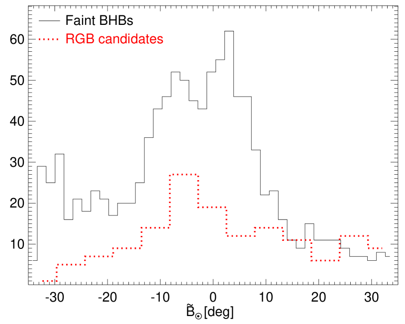
Figure 5: Across-stream profiles of the candidate members of the Sgr trailing stream in the North. The faint BHB stars (solid) and the spectroscopic RGBs (red dotted) in the range $145^{\circ}<\tilde{\Lambda}_{\odot}<170^{\circ}$ are shown. The BHB distribution appears double-peaked, while the more metal-rich RGB profile peaks at $\tilde{B}_{\odot}\sim-5^{\circ}$. This behaviour is reminiscent of the recent measurement of the trailing debris in the Galactic South by Koposov et al. (2012), who detect the similar metallicity difference between the stream components at positive and negative $\tilde{B}_{\odot}$.

To summarize, each of the three panels of Figure 2 shows the properties of a different stellar tracer inside the Sgr stream. The underlying logic that links the distribution of MSTO stars on the sky with the distance evolution of the BHBs and the kinematics of the RGB stars is threefold. First, the density enhancements in all three stellar populations are limited to the Sgr orbital plane as represented by the rotated coordinate system similar to that of Majewski et al. (2003). Second, both the BHB and the RGB overdensities are narrow enough to match the cross-section of the stream as measured on the celestial sphere. Third, as a function of the longitude $\tilde{\Lambda}_{\odot}$, the RGB kinematics evolves in agreement with the distance gradients as traced by the BHB stars. In particular, the LOS velocity of both the leading and the trailing tail goes through zero in the vicinity of the respective apo-centre.

2.3 Trailing arm: Connecting the dots

Given the clarity of the stream signal in both distance and the velocity domain, it is straightforward to measure the change in the centroid of the Sgr debris as a function of $\tilde{\Lambda}_{\odot}$. To this end, we build the model of the Galactic foreground and the Sgr stream as follows. At each $\tilde{\Lambda}_{\odot}$, the latitudinal probability that a star belongs to the stream is Gaussian, while the probability of belonging to the foreground changes linearly with latitude $\tilde{B}_{\odot}$. Therefore, there are 4 unknowns describing the centre and the width of the Gaussian and the slope and the normalization of foreground. The sets of 4 model parameters are allowed to evolve freely from bin to bin in longitude $\tilde{\Lambda}_{\odot}$. In each bin, the maximum likelihood model is sought using the individual BHB distance modulus values and the RGB velocity values with a brute-force grid search implemented in IDL. As is obvious from the Figure 2, the foreground density field is not exactly linear as a function of $\tilde{B}_{\odot}$. Therefore, when fitting the distance modulus signal, only values within $\pm 1$ mag of the tentative stream centroid were used. Similarly, while modelling the velocity, only the values inside $\pm 150$ km/s margin were used. The width of the bin in $\tilde{\Lambda}_{\odot}$ was chosen through trial and error to maintain reasonably high longitudinal resolution while having enough signal-to-noise per bin. The distances are measured in bins that are $4\aas@@fstack{\circ}7$ ($6\aas@@fstack{\circ}6$) wide, for the leading (trailing) arm respectively. The velocities are measured in bins that are $6\aas@@fstack{\circ}2$ ($7\aas@@fstack{\circ}05$) wide, for the leading (trailing) arm respectively. The distance and velocity centroids with the associated uncertainties are reported in Tables 1, 2 and 3, 4 and  5 respectively and shown in Figure 6.

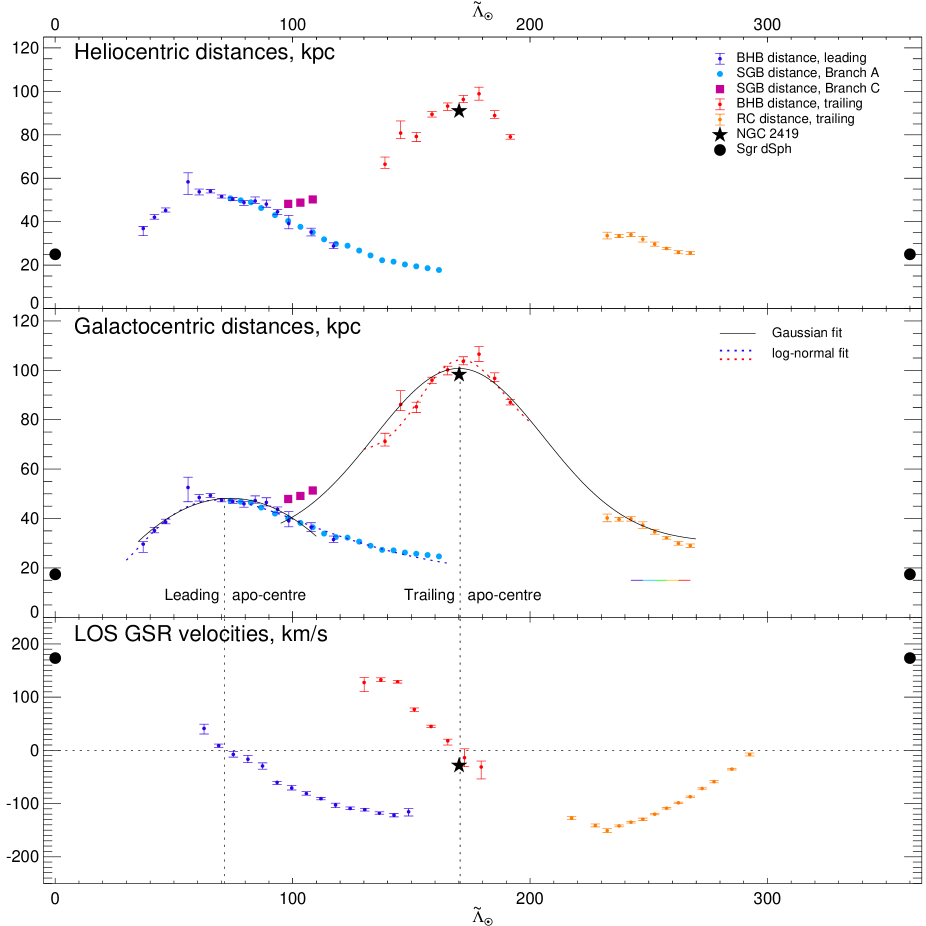
Figure 6: Distance and velocity measurements of the Sgr stream.Top: Violet (red) data-points with error bars show the centroid of the heliocentric distance of the stream debris at given longitude $\tilde{\Lambda}_{\odot}$ for the leading (trailing) tail. Blue (magenta) filled circles (squares) are SGB-based Branch A (C) distance measurements from Belokurov et al. (2006) increased by 0.15 mag to match the BHB signal. Orange data-points with error-bars are RGB-based distance measurements from Koposov et al. (2012) increased by 0.35 mag to correct for the reddening towards the progenitor. A black star marks the location of the globular cluster NGC 2419. Middle: Galactocentric stream distances. The stream is assumed to be at $B=0^{\circ}$ everywhere. While this will bias the run of distances for the individual branches of the leading arm at $\tilde{\Lambda}_{\odot}>150^{\circ}$, this is a very reasonable approximation for the debris around both apo-centres. Violet and red solid curves show the log-normal fits to the data, while black solid curves represent pure Gaussian models. Dotted lines mark the location of the leading and trailing apo-centres. Bottom: Measurements of the line-of-sight velocity $V_{\rm GSR}$ along the stream. The velocity centroids are those based on the SDSS giants stars as presented in Tables 3,  4 and  5. Note that the stream velocity appears to go through zero in the vicinity of the apo-centre.

Top and middle panels of Figure 6 show the distances to the centroids of the BHB stars in the Sgr stream measured as described above. Also shown are the distances measured using the stream’s Sub Giant Branch (SGB) stars, as reported by Belokurov et al. (2006). Note, however, that there is an important discrepancy between the SGB and the BHB measurements. The SGB distance moduli $(m-M)_{\rm SGB}$ needs to be increased by 0.15 mag to match the values of BHB distances at the same locations. The SGB measurements in Belokurov et al. (2006) are differential with respect to the main body of Sgr dSph and can be placed on the absolute scale only by assuming the overall metallicity of the Stream. Belokurov et al. (2006) suggested that the Stream’s stellar population resembles closely that of the remnant and hence assigned the same $i$-band magnitude to the SGB in the Stream and the Sgr core. The offset between the SGB and BHB stars measured here implies that the SGB of the Stream is 0.15 magnitudes brighter than the SGB of the remnant and hence more metal poor. This is in good agreement with the recent measurements of metallicity gradients along the Sgr stream (e.g. Bellazzini et al. 2006; Chou et al. 2007; Niederste-Ostholt et al. 2010). Alternatively, simply assuming the distance to the Sgr remnant of 26 kpc instead of 24 kpc produces a similar offset in $(m-M)$.

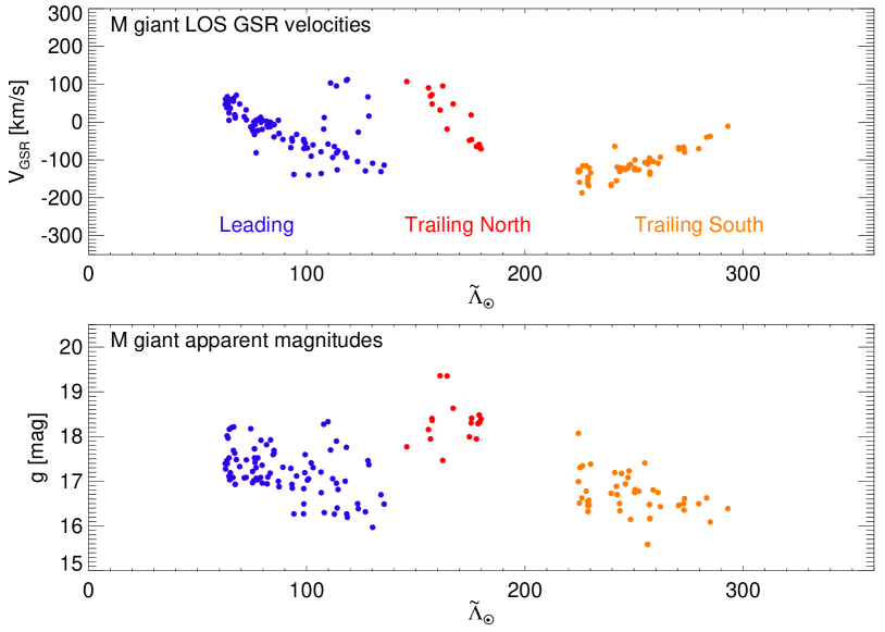
Figure 7: Top: Radial velocities of the M giant candidate stars with $-9^{\circ}<\tilde{B}_{\odot}<9^{\circ}$ selected using the criteria specified in equation 2 as a function of $\tilde{\Lambda}{\odot}$. The color-coding is used to emphasize the obvious velocity groups. The radial velocity trends match well those presented in Figures 2 and  6. Bottom: Apparent $g$ band magnitude of the selected M giant candidates as a function of $\tilde{\Lambda}_{\odot}$. The distance trends are similar to those reported in Figure 6. The large spread is the result the strong dependence of the M giant absolute magnitude on the temperature (color), the metallicity and the age. See text for the estimates of the M giant distances.

With the accurate distance measurements of the trailing debris covering $140^{\circ}<\tilde{\Lambda}_{\odot}<190^{\circ}$ reported here, it is easy to “connect the dots” and conclude that the most natural explanation for the so-called Branch C (see e.g. Belokurov et al., 2006; Fellhauer et al., 2006), confirmed most recently by Correnti et al. (2010) with Red Clump giants, is simply the extension of the trailing tail into the range of lower $\tilde{\Lambda}_{\odot}$ where it overlaps with the leading tail at $\tilde{\Lambda}_{\odot}\sim 100^{\circ}$. The trailing stream lies further out in the halo and follows a steeper distance gradient than predicted by any Sgr disruption model to date. For example, in the model of Law & Majewski (2010) the crossing of the leading and trailing tails in the North happens at RA$\sim 150^{\circ}$ or $\tilde{\Lambda}_{\odot}\sim 140^{\circ}$, thus missing it by some $40^{\circ}$. The available kinematics of the trailing tail lend support to our interpretation. The lower panel of Figure 6 shows that as the debris reach the apo-centre at $\tilde{\Lambda}_{\odot}\sim 170^{\circ}$, the LOS velocity changes sign and goes through zero. The maximum LOS velocity is reached at a point where the line of sight is best aligned with the stream. In the trailing arm velocity data, there is a clear indication of the plateau at $\tilde{\Lambda}_{\odot}\sim 135^{\circ}$. The LOS velocity is then expected to drop to zero close to the peri-centre, which for the trailing tail seems to lie not too far from the point of the crossing with the leading tail.

If the above interpretation is correct, then the Sgr trailing debris are flung out as far as 100 kpc away from the Galactic centre. This in turn implies a difference of $\sim 50$ kpc between the leading and the trailing apo-centres, which is not predicted by any of the current Sgr disruption models. While the orbital precession is sensitive to the global properties of the potential probed by the orbit, the difference in apo-central distances is also the consequence of the offset in energy and angular momentum of the debris at the moment of stripping, which for systems like Sgr, happens predominantly at peri-centre. A larger offset can be either a result of a steeper potential or a larger tidal diameter of the satellite, or indeed, a combination of both.

2.4 The M giant acid test

M giants are scant at high Galactic latitudes. Compared to the bulk of the Milky Way stellar halo, these stars are typically much younger (somewhere in the range of 4 to 8 Gyr) and more metal-rich. Given their distinct infrared and ultraviolet colors, M giants can be identified easily, and provided the redder and therefore more metal-rich sub-sample is selected, will generally suffer very low levels of contamination. As exemplified by the studies of Majewski et al. (2003) and Yanny et al. (2009), M giants are ideal markers to track down the Sgr tidal debris across the sky. Crucially, for our study, compared to the older and the more metal-poor BHBs and the RGBs, they represent a well-studied, largely complementary stellar tracer population with high purity.

As Figure 3 demonstrates, in the SDSS spectroscopic dataset, M giant candidates can be picked out using the following selection criteria.

$$\begin{split}4,000<T_{eff}<4,600K\\ 1<\mathrm{log}(g)<2.2\\ 2.7<u-g<3.5\\ -2<[Fe/H]<0\end{split}$$ (2)

Figure 7 shows two distributions of the M giant candidate stars with $-9^{\circ}<\tilde{B}_{\odot}<9^{\circ}$ selected using the above criteria. The data-points are split into three groups according to the range of $\tilde{\Lambda}_{\odot}$ they inhabit, as indicated by the color coding. Top panel of Figure 7 gives the M giant locations on the plane of the line-of-sight velocity (corrected for the solar reflex motion) and the stream longitude $\tilde{\Lambda}_{\odot}$. It is evident that the absolute majority of the stars plotted do belong to the Sgr tidal tails. Indeed the contamination is minimal as there are only few M giants in the range $100^{\circ}<\tilde{\Lambda}_{\odot}<140^{\circ}$ that deviate from the radial velocity trends presented in Figure 6. In fact, perhaps some of these “contaminating” stars are part of the Branch C of the stream, i.e. the continuation of the trailing tail to lower $\tilde{\Lambda}_{\odot}$. Most importantly, the M giant radial velocity signature at $140^{\circ}<\tilde{\Lambda}_{\odot}<190^{\circ}$ matches perfectly the RGB kinematics presented in the lower panel of Figure 6. For example, the M giant radial velocity signal goes through zero around $\tilde{\Lambda}_{\odot}\sim 170^{\circ}$.

An idea of the heliocentric distance of the stream’s M giants can be gleaned from the Bottom panel of Figure 7. Here, the apparent $g$ band magnitude of the selected stars is plotted as a function of the longitude $\tilde{\Lambda}_{\odot}$. While the data-points follow the general distance trends shown in the Top panel of Figure 6, the scatter is substantial. This is because the intrinsic luminosity of an M giant star varies significantly with its temperature (and hence color), as well as the metallicity and the age. Using the BHB stars in the Sgr stream around $\tilde{\Lambda}_{\odot}\sim 75^{\circ}$, Yanny et al. (2009) obtained $M_{g}=-1$ for the stream’s M giants. Using this simple absolute magnitude calibration we can obtain a crude estimate of the helio-centric distance to the 19 M giant candidate stars in the range $140^{\circ}<\tilde{\Lambda}_{\odot}<190^{\circ}$. Their mean $g$ band apparent magnitude is 18.4 and the dispersion is 0.4 mag. If there was no strong metallicity/age gradient along the stream, applying the absolute magnitude calibration of Yanny et al. (2009) leads to the distance estimate of 75${}^{+15}_{-10}$ kpc. This is slightly lower but overall consistent with the distance estimate to the BHB stars in the same range of $\tilde{\Lambda}_{\odot}$. However, the assumption of the zero gradient in the stream’s stellar populations is perhaps too naive as shown in Figure 8. The top panel of the Figure shows the distributions of the metallicity (as derived by the SDSS SSPP pipeline) of the M giant stars selected to lie in the three $\tilde{\Lambda}_{\odot}$ ranges as indicated in Figure 7. There is a pronounced gradient in $[Fe/H]$ between the Southern and the Northern trailing debris, with the mean metallicity shifting from -0.7 to -1.1. The metallicity distributions of the leading tail and the distant trailing tail agree much better, but the average values of $[Fe/H]$ still differ by 0.15 dex. As illustrated in the lower panel of Figure 8, even 0.15 dex lower metallicity can result in $\sim$ 0.5 mag larger distance modulus. This would imply that the average distance to the faint M giant stars could be closer to $\sim 95$ kpc.

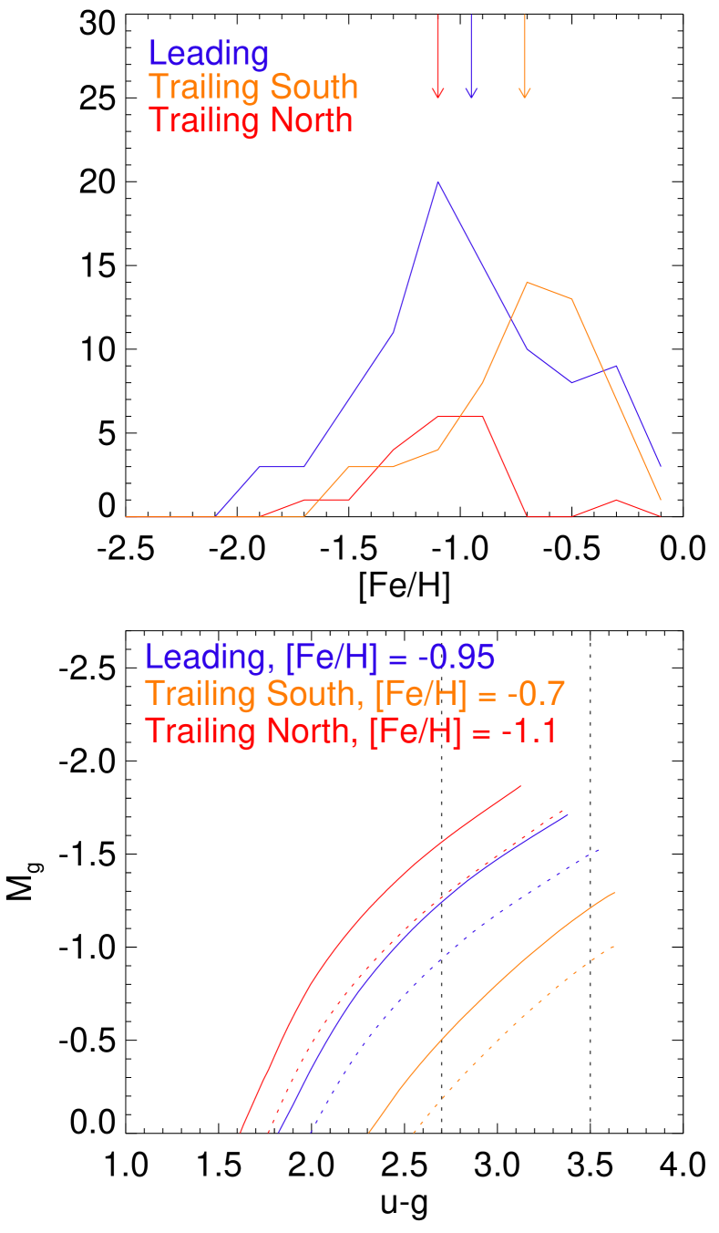
Figure 8: Top: Metallicity distributions of the M giant stars in the three $\tilde{\Lambda}_{\odot}$ ranges, as indicated in Figure 7. The arrows give the mean metallicity values for each M giant sub-sample. Note, that there is a significant downward shift in mean $[Fe/H]$ between the Southern (orange) and the Northern (red) detections of the trailing tail. The $[Fe/H]$ distribution of the leading tail (blue) agrees better with the distant trailing debris (red); yet there is a 0.15 dex difference in mean metallicities of the two M giant groups. Bottom: Dartmouth theoretical isochrones (Dotter et al., 2008) shown for the three mean M giant metallicities for 4 Gyr (solid) and 8 Gyr (dotted) populations. Note that even 0.15 dex difference in $[Fe/H]$ can result in $\sim$0.5 mag difference in absolute magnitude.

Overall, the M giants provide strong support to the picture drawn with other SDSS stellar tracers. In particular, in the portion of the sky in question, i.e. in the range of $140^{\circ}<\tilde{\Lambda}_{\odot}<190^{\circ}$, the M giants, BHBs and RGB follow essentially identical velocity and distance trends.

3 NGC 2419

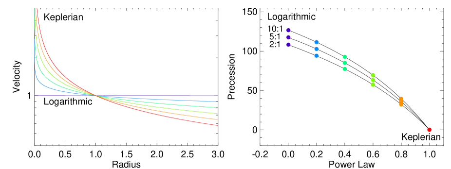
Figure 9: Left: Circular velocity curves in power-law potentials as a function of radius. Right: Apo-centre to apo-centre precession in power-law potentials as a function of the power for three different eccentricities. For each potential (colour-coded according to power-law index), the precession angle in degrees is shown for three orbits with the ratio of apo-centric to peri-centric distance of 10:1, 5:1 and 2:1.

NGC 2419 is rather unusual for a Milky Way globular cluster. Together with $\omega$Cen, it deviates from the size-luminosity relation obeyed by other Galactic globulars, as noted, for example, by van den Bergh & Mackey (2004). NGC 2419 appears to have a relaxation time well in excess of Hubble time. In other words, it is much too extended for its stellar mass, which by itself makes it one the most luminous GCs in the Galaxy. van den Bergh & Mackey (2004) and others have noted the resemblance between NGC 2419, $\omega$ Centauri and M54 and suggested that these clusters could have formed and evolved in dwarf satellites of the Milky Way which were then destroyed during accretion leaving the fleshy clusters intact in the gravitational field of the Milky Way. Accordingly, the search is on for evidence of the past existence of the globular’s parent galaxy. van den Bergh & Mackey (2004) predict a spread, albeit possibly quite small, in the metallicities of the cluster’s member stars. Most recently, Cohen et al. (2010) seem, at first glance, to have detected exactly that: a small, but measurable spread in the CaT equivalent widths of several tens of the RGB stars in NGC 2419, which could be interpreted as the spread in $[{\rm Fe}/{\rm H}]$ values around the mean of $-2.1$. However, in the follow-up high resolution study, Cohen et al. (2011) and Cohen & Kirby (2012) find no detectable spread in $[{\rm Fe}/{\rm H}]$, but unusually high depletion of Mg and a bizarre anti-correlation between Mg and K. They conclude by stating that no nucleosynthetic source is capable of explaining the chemical makeup of NGC 2419.

Of course, any sign of the tidal debris that can be traced back to the vicinity of NGC 2419 would be a giveaway just as well. Newberg et al. (2003) show that, within the Sgr debris plane, an overdensity of BHBs at distances similar to that of NGC 2419 can be seen in the SDSS photometric data. The significance of this BHB overdensity was confirmed recently by Ruhland et al. (2011). Given the proximity of the stream and the cluster, Newberg et al. (2003) speculate that the cluster was once part of the Sgr galaxy. Casetti-Dinescu et al. (2009) on the other hand link the cluster with the Virgo Stellar Stream (which is, most likely, a part of the Virgo Over-Density) on the basis of the cluster’s proximity to the very eccentric orbit predicted from the measured mean radial velocity and the proper motion of the stream. In this paper, we have shown that NGC 2419 does lie close to the plane of the Sgr tidal debris. According to Figure 4, NGC 2419 is situated near the edge of the stream at $\tilde{B}_{\odot}\sim 9^{\circ}$. Figures 6 and 10 show that NGC 2419 is located right at the apo-centre of the Sgr trailing debris, more than 100 kpc away from the remnant. Finally, the cluster’s LOS velocity matches that of the receding trailing debris reaching its apo-centre. If this globular was indeed part of the Sgr dwarf in the distant past, it might not be too surprising that presently it is found further away from both the centroid of the stream and the remnant itself. Had it lived closer to the central parts of Sgr, chances are it would have fallen into the centre of the dwarf galaxy due to the dynamical friction.

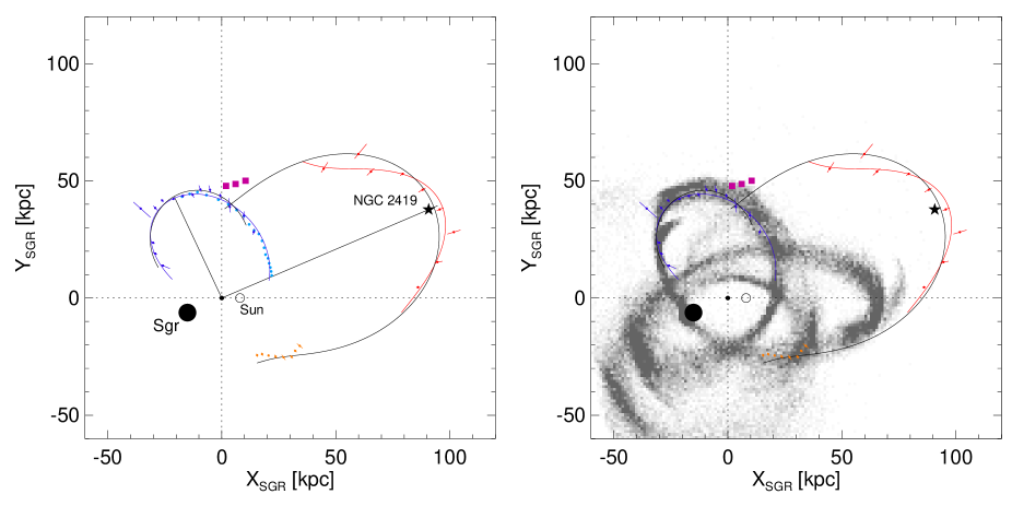
Figure 10: Stream precession in the plane of the Sgr orbit. The plane chosen has its pole at Galactocentric $l_{\rm GC}=275^{\circ}$ and $b_{\rm GC}=-14^{\circ}$. All symbols, colours and curves are identical to those in Figure 6. Left: Note that the actual Galactocentric orbital precession of $93^{\circ}$ is slightly lower than the difference between the heliocentric apo-centre phases from Figure 6. Right: Comparison with the Sgr disruption model by Law & Majewski (2010) shown as grey-scale density. Note that in the logarithmic halo used in the model, the orbital precession is $\sim 120^{\circ}$ and the trailing apo-centre lies in the Galactic disk at $\tilde{B}_{\rm GC}^{\rm T}\sim 0^{\circ}$ and distance of $R^{\rm T}\sim 65$ kpc. This should be contrasted with the new measurement of $\tilde{B}_{\rm GC}^{\rm T}\sim 23^{\circ}$ and $R^{\rm T}=102.5\pm 2.5$ kpc.

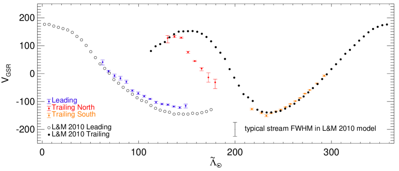
Figure 11: Measurements of the Sgr stream radial velocity (colored data points) and the predictions of the Law & Majewski (2010) disruption model (filled and empty circles). In each bin of $\tilde{\Lambda}_{\odot}$, the centroid of the model debris is given by the median particle velocity. The agreement between the data and the model is perfect in the South. The kinematics of the leading tail in the North is also reproduced fairly well, although there seems to be a systematic offset of order of $\sim$20 km s^-1. This offset is however smaller than the breadth of the model tidal debris as indicated by the stand-alone black error-bar. The most significant discrepancy is between the distant trailing tail data (red) and the model prediction (filled circles) in the range $130^{\circ}<\tilde{\Lambda}_{\odot}<190^{\circ}$.

There is a slight hint of bimodality in the distribution of the distant BHBs at around $\tilde{\Lambda}\sim 160^{\circ}$ in the Left panel of Figure 4. This is confirmed in the across-stream distribution of the BHBs shown in Figure 5. The width of this part of the trailing stream on the sky is $\sim 20^{\circ}$. This is consistent with the detections of the Sgr debris everywhere else on the celestial sphere. However, everywhere else, these $\sim 20^{\circ}$ are made up of two distinct components: Branch A and B around the North Galactic Cap (Belokurov et al., 2006), bright and faint trailing stream in the South (Koposov et al., 2012). As judged by the latitude of NGC 2419 in the Sgr coordinate system, it lies much closer to the debris plane defined by the faint companion to the trailing tail. According to Koposov et al. (2012) this newly-found stream is metal-poor which helps to strengthen its link to NGC 2419 which possesses $[{\rm Fe}/{\rm H}]\sim-2.1$.

There are examples of globular clusters as extended as NGC 2419 outside the Milky Way. Brodie et al. (2011) discovered a population of low-surface brightness counterparts to Ultra Compact Dwarfs in M87, spanning a similar range in size and luminosity. Huxor et al. (2005) discovered a population of faint ($M_{V}\gtrsim-7$) and fuzzy globulars with typical sizes $\sim 30$pc in the neighboring spiral M31. Interestingly, Mackey et al. (2010) showed that all but one of these extended clusters in Andromeda’s outer halo lie - in projection - within the known tidal streams. This points to the dwarf satellites of luminous galaxies as the birth place of extended clusters, at least the ones similar to those discovered by Huxor et al. (2005). Some evidence to support this hypothesis has been published recently. Da Costa et al. (2009) presented a discovery of an extended globular cluster in a low luminosity dwarf ellipitical member of the Virgo group. There are also hints of bimodality in the size distribution of globular clusters in dwarf galaxies in the Local Volume (Georgiev et al., 2009).

With its unusually high (for a Milky Way globular cluster) luminosity of $M_{\rm V}=-9.4$, NGC 2419 may have more in common with so-called Ultra-Compact Dwarf (UCD) galaxies (Drinkwater et al., 2000) than with extended globular clusters. However, not only are the UCDs at least a magnitude more luminous, they also appear to have somewhat inflated velocity dispersions, as evident from the inferred mass-to-light ratios of $\sim 5-10$ similar to that of the nuclei of dwarf ellipticals in clusters of galaxies (e.g. Geha et al. 2002). It is therefore not surprising that one of the more popular UCD formation scenarios involves tidally stripping a dwarf elliptical. As of today, the progenitors of the UCDs have not yet been established with certainty. Also, as Haşegan et al. (2005) show, it is close to impossible to assign an astrophysical class to an object in a certain range of luminosity, size and velocity dispersion as quite a few “dwarf-globular transition objects” exist with properties in between globular clusters and dwarf galaxies. Even though a whole zoo of such transition objects have been uncovered elsewhere, in the Milky Way NGC 2419 is in a class of its own: too luminous but not dense enough for a globular, close to the faint end of UCDs, yet, as has been shown by Baumgardt et al. (2009), it can not boast a mass-to-light ratio out of ordinary.

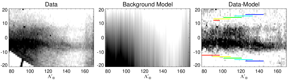
Figure 12: Foreground model subtraction for the debris plane analysis.Left: Density of the MSTO stars in the coordinate system with the pole at $l=99\aas@@fstack{\circ}7$, $b=13\aas@@fstack{\circ}7$ to ensure that both Branch A and B lie at approximately constant latitude. Middle: Foreground stellar density modelled as constant slope for each column of the density presented in Left panel. The slope is allowed to vary as a function of the longitude $\Lambda_{\odot}^{\prime}$ Right: Branches A and B revealed after the foreground subtraction. Coloured lines show the sections of the stream used for the debris plane calculation (see Figure 13).

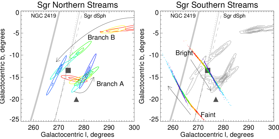
Figure 13: Precession of the plane of the Sgr debris in Galactocentric $l$ and $b$ coordinates. Three black lines crossing each panel show the great circles drawn by the poles of the planes passing through the current position of the Sgr remnant. Solid is for the Sgr dSph heliocentric distance of 25 kpc, while dotted (dashed) is for the distance increased (reduced) by 5 kpc. Thick light grey line gives the great circle of planes passing through NGC 2419. Left: Two sets of contours mark the peaks in the pole density (99.4% and 99.9%) for the five over-lapping sections of the two branches of the leading stream (as indicated in the Right panel of Figure 12). Filled square (triangle) shows the debris plane of the trailing (leading) stream as reported by Johnston et al. (2005). Note the evolution of the leading stream plane away from the trailing pole towards increasing $l$ and the possible turn-over at $l_{\rm GC}\sim 280^{\circ}$ towards decreasing $b_{\rm GC}$. The amplitude of the plane precession is markedly different for Branches A and B. Also, note that the two branches have the opposing sense of the plane precession. Right: Plane precession for both bright and faint Sgr trailing streams. The Gaussian scatter in distance and $B$ is added to the stream centroids of pairs of detections reported by Koposov et al. (2012), each coloured point then gives the debris pole determined. There are 300 realisations for each of the 5 pairs of $\tilde{\Lambda}_{\odot}$. The colour changes in the fashion similar to that of the Left panel: from red to dark blue in the direction of the Sgr motion (also see Middle panel of Figure 6 for exact $\tilde{\Lambda}_{\odot}$ values). While the precession of the bright trailing debris is consistent with that of the debris in Branch A of the leading tail, the debris in the faint trailing stream component precesses in the direction opposite to its bright counterpart.

The genesis of either the faint component of the Sgr stream or NGC 2419 is yet to be established. This paper shows that in 4 out of 6 phase-space coordinates, the stream and the cluster are coincident. The recent discovery of highly peculiar elemental abundances in this cluster by Cohen & Kirby (2012) presents a rare opportunity to verify the connection between the two.

4 The precession of the Sagittarius debris

4.1 Orbital precession

The rate with which an orbit precesses in a spherically symmetric gravitational potential depends primarily on how quickly the mass generating the gravity field decays with radius. For example, in Keplerian potentials, the precession angle is $0^{\circ}$ to ensure the orbits are closed after one period, while in logarithmic haloes, the precession is $\sim 120^{\circ}$. Orbits in the outer regions of spherical galaxies should posses a precession rate somewhere between $0^{\circ}$ and $\sim 120^{\circ}$. The precession rate is not solely dependent on the mass decay rate in the host, it is also a weak function of the orbital energy and angular momentum (see equation 3.18 in Binney & Tremaine 2008). The dependence of the orbital precession on the potential and the eccentricity of the orbit is illustrated in Figure 9. The left panel of the Figure shows rotation curves for the family of power law potentials $\Psi=-\alpha^{-1}r^{-\alpha}$ for various $\alpha$. The right panel shows the angle between the successive apo-centre passages in the potential with given $\alpha$, for three orbital eccentricities. As can be seen from Figure 9, the precession angle increases as the potential gets flatter. This increase is steeper for more eccentric orbits.

It is not possible to measure the precession of the Sgr progenitor’s orbit directly, but the angle between the leading and the trailing apo-centres encodes the necessary information. The angle between the two apo-centres detected in the SDSS data is calculated as follows. Two simple models are fitted to the Sgr Galactocentric distance data: Gaussian and log-normal. While both are completely unphysical, these describe the available data satisfactorily and give an idea of the uncertainty associated with the model mismatch. Overall, the distance to the trailing debris appears to be more Gaussian-like, therefore the Gaussian model is fitted to all the data presented in the top panel of Figure 6. Around the apo-centre, there is a clear asymmetry in the run of the distances, hence the log-normal model is fitted for the range $130^{\circ}<\tilde{\Lambda}_{\odot}<200^{\circ}$. The opposite is true for the leading tail data: the entire tail is modelled as log-normal, while Gaussian is fitted to the distances in the range $35^{\circ}<\tilde{\Lambda}_{\odot}<110^{\circ}$. For each of the tails, the average of the two model values for the location of the apo-centre is taken.

Solid lines of different colour show the best-fit models for both tails in the middle panel of Figure 6. For the leading tail, the black line is the Gaussian and the blue curve is the log-normal. The leading apo-centre is at $\tilde{\Lambda}_{\odot}^{\rm L}=71\aas@@fstack{\circ}3\pm 3\aas@@fstack{\circ}5$, where it reaches $R^{\rm L}=47.8\pm 0.5$ kpc. Trailing tail’s apo-centre is at $\tilde{\Lambda}_{\odot}^{\rm T}=170\aas@@fstack{\circ}5\pm 1^{\circ}$ and $R^{\rm T}=102.5\pm 2.5$ kpc. The red curve shows the log-normal model, while black is the Gaussian. In the heliocentric coordinate system of Majewski et al. (2003), the differential orbital precession between the leading and the trailing apo-centres is $\delta\tilde{\Lambda}_{\odot}=99\aas@@fstack{\circ}3\pm 3\aas@@fstack{\circ}5$. Taking into account the Sun’s distance from the center of the Galaxy $R_{0}=8$ kpc, the Galactocentric $\delta\tilde{\Lambda}_{\rm GC}=93\aas@@fstack{\circ}2\pm 3\aas@@fstack{\circ}5$.

Figure 10 shows the Sgr stream detections presented in Figure 6 now in the debris plane defined by the pole at $(l_{\rm GC},b_{\rm GC})=(275^{\circ},-14^{\circ})$. The right panel of the Figure compares the current data with the model by Law & Majewski (2010) projected onto the same plane. While most of the data, including the entirety of the leading tail detections and the trailing tail data in the range $220^{\circ}<\tilde{\Lambda}_{\odot}<280^{\circ}$ is reproduced by the model extremely well, the distant trailing tail measurements in the range $100^{\circ}<\tilde{\Lambda}_{\odot}<200^{\circ}$ clearly do not have any counterpart in this simulation. Both the distance to the trailing apo-centre and its position angle are at odds with the observations. Figure 11 illustrates the model-data mismatch further by displaying the run of the measured radial velocity of both Sgr leading and trailing tidal tails as well as the evolution of the LOS velocity centroid in the Sgr disruption model of Law & Majewski (2010). While the model agrees perfectly with the kinematic data at $220^{\circ}<\tilde{\Lambda}_{\odot}<300^{\circ}$, there is a small systematic offset at $80^{\circ}<\tilde{\Lambda}_{\odot}<150^{\circ}$, but a pronounced gap at $150^{\circ}<\tilde{\Lambda}_{\odot}<190^{\circ}$. At first glance, it seems that the new data presented here require the Galactic halo mass to drop faster with increasing radius than imposed by the logarithmic model used by Law & Majewski (2010). The matter of inferring the Galactic mass constraints from the Sgr debris detections presented here will be addressed thoroughly in a separate publication (Gibbons et al, in prep.)

4.2 Orbital plane precession

The previous Subsection assumed implicitly that the leading and the trailing debris, at least up to their respective apo-centres, stay within the same plane, namely the one defined by $(l_{\rm GC},b_{\rm GC})=(275^{\circ},-14^{\circ})$. Is this a reasonable assumption? How fast does the plane of the debris precess? Johnston et al. (2005) show that the M giants in the leading and the trailing tail define Galactocentric planes whose poles are $\sim 10^{\circ}$ apart. Taking advantage of the dramatic increase in the depth of the SDSS survey compared to 2MASS, as well as the accurate stream distances based on the BHB stars, it is timely to update the study of the evolution of the plane of the Sgr debris.

Most of the new information supplied by the SDSS is in the North, and so it is the leading tail plane evolution we will concentrate on. We start by removing the Galactic foreground contribution from the distribution of the MSTO star counts. This is done in the coordinate system similar to the one used above, but rotated slightly to ensure that both branches of the leading tail run at constant latitude throughout the range of longitudes seen by the SDSS (see Left panel of Figure 12). Specifically, this is the plane defined by the pole with $(l,b)=(99\aas@@fstack{\circ}7,13\aas@@fstack{\circ}7)$. In each pixel of the longitude $\Lambda_{\odot}^{\prime}$, the foreground density is fitted with a linear model. Only the pixels outside the range $-8^{\circ}<B_{\odot}^{\prime}<10^{\circ}$ are taken into account during the fit. The resulting model foreground is shown in the Middle panel of Figure 12. The residuals of the model subtraction are shown in the Right panel of the Figure. With the foreground (dominated by the Virgo stellar cloud) gone, the leading stream appears with particular clarity.

Each pixel in the right panel of Figure 12 is a line in the space of poles of Galactocentric planes, provided its distance is known. The superposition of such lines defines the cloud of poles corresponding to the group of pixels on the sky. Note that the pole lines each carry a weight according to the stellar density of the pixel they correspond to. We split Branches A and B into 5 overlapping pieces with the boundaries marked in colour and shown below and above each branch respectively, and map the stellar density in each of the pieces onto the debris pole plane using the method above. Left panel of Figure 13 gives the contours of the pole density for each piece of Branch A and B. Pixels belonging to each branch are selected using the simple condition of $B_{\odot}^{\prime}<0$ for Branch A, and $B_{\odot}^{\prime}>0$ for Branch B. The colour-coding used here is identical to the colour-coding in the Right panel of Figure 12. Also plotted here are the two measurements based on the M giants of the trailing and the leading pole reported in Johnston et al. (2005), marked by filled square and triangle respectively. The three lines crossing the figure are the lines of poles of the planes passing through the current position of the remnant. The difference between the lines is the assumed distance to the Sgr dSph.

The earliest it is possible to register the pole of the leading debris is some $\sim 80^{\circ}$ away from the remnant. As shown by the red contours, at this stage, the leading debris has already precessed away several degrees from the plane defined by the M giants in the trailing tail. The precession of the leading pole is in the direction of increasing $l_{\rm GC}$ and decreasing $b_{\rm GC}$, the same direction as identified by Johnston et al. (2005). As we step along the Branch A, the debris pole first moves further in the same direction, but then turns before reaching the position determined using the M giants. It is unclear whether this turn-around is real as most of the lines in the space of poles contributed by pixels in the segments of the tail at $\Lambda_{\odot}^{\prime}>120^{\circ}$ are closely aligned as can be gleaned from the shapes of the contours. The signature of the same degeneracy can be seen in the top panels of Figure 3 of Johnston et al. (2005). Nonetheless, we can conclude with certainty that the amplitude of the precession of the plane of the leading debris over $\sim 100^{\circ}$ along the stream ought to be less than $\sim 10^{\circ}$.

The evolution of the debris plane defined by the pixels in Branch B is surprisingly different from that of Branch A. The density contours are even more stretched, making it difficult to pinpoint the exact position of the pole for each section of the stream. However, the broad-brush behaviour is apparent: the sense of precession of the Branch B debris pole is opposite to that of Branch A. As one steps along the leading tail away from the remnant in the direction of Sgr motion, the Branch B pole moves in the direction of decreasing $l$ and decreasing $b$.

In the South, we do not perform the full debris mapping into the space of the orbital poles, as the SDSS coverage of the stream is limited. Instead, we compute the poles of the planes defined by the pairs of the first 6 detections given in Table 2 of Koposov et al. (2012) . For each such pair, 300 Monte-Carlo trials are carried out to propagate the distance and the latitude $\tilde{B}_{\odot}$ uncertainty. The resulting debris poles are shown as elongated clouds of dots, whose colour-coding is explained in the Middle panel of Figure 6. The colour changes from red to light blue in the direction of the Sgr motion, similar to the colour-coding scheme used for the leading tail study above. It is reassuring to see that the mean of the five debris pole clouds generated using the bright component of the trailing stream shown in the Figure lies very close to the value of Johnston et al. (2005). Overall, the poles of the debris in the bright trailing stream at $240^{\circ}<\tilde{\Lambda}_{\odot}<280^{\circ}$ have the same sense of precession as the Branch A debris around $80^{\circ}<\tilde{\Lambda}_{\odot}<100^{\circ}$, i.e. the stream angular momentum vector moves in the direction of increasing $l$ and decreasing $b$. Once again, the faint component of trailing stream shows the sense of precession opposite to the bright portion of the tail: the pole moves in the direction of decreasing $l$ and increasing $b$.

Finally, the poles of the debris planes at the positions of the apo-centres seem to lie very close to each other, as judged by the Branch A red contours in the Left panel and dark blue and light blue dots (for the Bright arm) in the Right panel, and reassuringly close to the pole of $275^{\circ},-14^{\circ}$ chosen for orbit mapping in Section 4.1.

Table 1: Heliocentric distances to the Sgr Leading stream based on the BHB detections.

$\Lambda_{\odot}$	37.1	41.8	46.5	55.9	60.6	65.4	70.1	74.8	79.5	84.2	88.9	93.6	98.4	107.8	117.2
$(m-M)_{0}$	17.83	18.12	18.27	18.83	18.65	18.66	18.56	18.51	18.44	18.47	18.41	18.25	17.96	17.73	17.30
$\sigma_{-}$	0.20	0.05	0.04	0.23	0.06	0.03	0.03	0.03	0.06	0.05	0.07	0.06	0.14	0.11	0.09
$\sigma_{+}$	0.06	0.06	0.05	0.15	0.05	0.03	0.03	0.03	0.04	0.08	0.08	0.05	0.20	0.11	0.11

Table 2: Heliocentric distances to the Sgr Trailing stream based on the BHB detections.

$\Lambda_{\odot}$	138.9	145.5	152.1	158.7	165.3	171.9	178.5	185.1	191.7
$(m-M)_{0}$	19.11	19.54	19.49	19.76	19.85	19.92	19.98	19.74	19.49
$\sigma_{-}$	0.06	0.07	0.07	0.03	0.05	0.03	0.07	0.03	0.03
$\sigma_{+}$	0.11	0.15	0.05	0.03	0.03	0.04	0.07	0.05	0.03

Table 3: Galactocentric velocities of the Sgr Leading stream based on the giant star detections.

$\Lambda_{\odot}$	62.7	68.8	75.0	81.2	87.3	93.5	99.6	105.8	111.9	118.1	124.2	130.4	136.5	142.7	148.8
$V_{\rm GSR}$	41.1	8.8	-7.6	-16.7	-29.5	-60.2	-70.7	-81.3	-90.8	-102.7	-109.2	-111.6	-118.3	-121.7	-115.5
$\sigma_{-}$	10.4	3.4	5.1	6.4	5.9	4.4	3.9	2.9	2.1	5.0	2.4	2.4	1.7	3.4	7.9
$\sigma_{+}$	7.9	3.0	5.8	7.0	6.0	1.8	4.9	3.5	2.2	3.4	2.7	2.6	2.8	2.9	6.1

Table 4: Galactocentric velocities of the Northern Sgr Trailing stream based on the giant star detections.

$\Lambda_{\odot}$	130.1	137.2	144.2	151.2	158.3	165.3	172.4	179.4
$V_{\rm GSR}$	127.4	132.5	128.8	77.0	44.7	17.8	-13.8	-31.3
$\sigma_{-}$	17.1	3.6	2.5	4.4	1.5	7.9	17.0	22.4
$\sigma_{+}$	9.3	3.6	2.1	2.7	2.5	3.1	16.6	11.2

Table 5: Galactocentric velocities of the Southern Sgr Trailing stream based on the giant star detections.

$\Lambda_{\odot}$	217.5	227.5	232.5	237.5	242.5	247.5	252.5	257.5	262.5	267.5	272.5	277.5	285.0	292.5
$V_{\rm GSR}$	-127.2	-141.1	-150.8	-141.9	-135.1	-129.5	-120.0	-108.8	-98.6	-87.2	-71.8	-58.8	-35.4	-7.8
$\sigma_{-}$	3.1	2.7	3.6	1.8	1.6	2.1	1.2	1.4	1.2	1.2	1.3	2.1	1.6	2.8
$\sigma_{+}$	3.1	2.7	3.6	1.8	1.6	2.1	1.2	1.4	1.2	1.2	1.3	2.1	1.6	2.8

5 Discussion and Conclusions

We have taken a Swiss Army Knife approach to the SDSS database and mapped the Sgr stellar stream across the sky using three stellar tracers. The MSTO stars helped us define the plane of the Sgr debris, the BHBs provided accurate distances, and the giants (mostly K and M) gave the clearest view to date of the kinematics of both the leading and the trailing tails as far as 100 kpc in the Galactic halo. Here, is the summary of our main conclusions.

(1) As we push the SDSS data to its limits, that is to the edge of the survey footprint, we are able to discern the apo-centres of the leading and the trailing streams. Distant Sgr debris reported previously by Newberg et al. (2003), Ruhland et al. (2011) and Belokurov et al. (2006) link with the new BHB detections to reveal the wide arc of the trailing tail.

(2) Both the orbital precession of the trailing debris and the Galactocentric distances it reaches are at odds with the current state-of-the-art models of Sgr disruption. The angle between the leading and the trailing apo-centres is $\delta\tilde{\Lambda}_{\rm GC}=93\aas@@fstack{\circ}2\pm 3\aas@@fstack{\circ}5$, while their respective distances are $R^{\rm L}=47.8\pm 0.5$ kpc $R^{\rm T}=102.5\pm 2.5$ kpc.

(3) We substantiate the detections of the tidal tails and their 3D evolution with the measurements of the debris’ line of sight velocity. In particular, we show that around the apo-centres stream’s $V_{\rm GSR}$ passes through zero.

(4) We demonstrate that a highly pure sample of spectroscopic M giant stars can be extracted from the SDSS data. Across the entire sky, but more importantly in the range $140^{\circ}<\tilde{\Lambda}_{\odot}<190^{\circ}$, these stars appear to provide a strong independent verification of both the distance and the velocity signals uncovered with the help of the BHBs and the RGBs.

(5) We show that in 4 out of 6 phase-space coordinates, the peculiar globular cluster NGC 2419 and the Sgr trailing tail coincide. NGC 2419 lies very close to the trailing apo-centre, nearer to the edge of the stream. Given its position and the chemical abundance, it is not impossible that the globular is in fact related to the faint, metal-poor companion of the trailing tail discovered by Koposov et al. (2012).

(6) The plane of the debris delineated by the MSTO stars and anchored with the BHB distances evolves slowly, but noticeably, in the Galactic potential. We also detect a turn-over in the path of the angular momentum of the leading tail.

(7) The sense of precession of the debris plane of both secondary components to the stream, Branch B in the North and the faint trailing tail in the South, appears to be opposite to the main, bright parts of the stream.

Here, we have measured the Galactocentric angle between the apocentres of the leading and trailing tails of the Sgr stream and the difference between their respective distances. The angle through which the orbit turns from one apocentre to the next is largely controlled by the radial profile of the potential. Our measured value is inconsistent with a flat rotation curve, or logarithmic potential, and indicates that the Milky Way’s dark matter density falls off more quickly than isothermal. We have also detected the precession of the orbital plane of the Sgr stream. This wallowing, or gentle nutation, of the orbital plane occurs naturally in mildly triaxial potentials, for which evidence exists on other grounds for the Milky Way (e.g., Debattista et al. 2013). In practice, the components of the Sgr progenitor most likely possessed some internal rotation or spin (e.g., Peñarrubia et al. 2010), which can couple to the torques provided by the triaxiality. The complex behaviour of the precession of the plane of the Sgr debris that we have measured is most likely caused by an interplay between the rotational kinematics of the stripped material and the torques exerted by the triaxial gravity field.

It is crucial to note, however, that without observing the uninterrupted connection between the Southern and the Northern stellar debris, it is impossible to say with 100% certainty that the structure visible in the SDSS data at $140^{\circ}<\tilde{\Lambda}_{\odot}<190^{\circ}$ is indeed the extension of the Sgr trailing arm. A range of other, admittedly less likely (as illustrated in Section 3), options can not be ruled out at the moment. Amongst these are: the contamination by other, previously unknown distant stellar halo sub-structure; a stream from a yet undiscovered companion body, presumably infalling in-sync with the Sgr dwarf. Encouragingly, as Figure 11 illustrates, the future line-of-sight velocity measurements in the range $190^{\circ}<\tilde{\Lambda}_{\odot}<210^{\circ}$ will provide a helpful discriminant: in this part of the sky, the current disruption models and the predictions from our analysis start to diverge drastically.

Above all, this study has uncovered the stupendous scale of the Sgr stream. The debris stretches over Galactocentric radii from roughly 20 kpc out to at least 100 kpc. This makes the Sgr stream the single most powerful probe of the Milky Way’s dark halo. It extends well beyond the gas rotation curve, which gives out at 20 kpc. As the Sgr stream also possesses abundant bright tracers like BHBs, accurate distances and velocities are obtainable almost everywhere. Provided we can decode the message in its runes, it offers momentous constraints on the underlying gravity field at unprecedentedly remote distances. It truly is a touchstone for studies of the very distant dark halo.

Appendix A Coordinate transformation

Here, we provide the equations for converting Equatorial ($\alpha$, $\delta$) to the Sgr stream coordinate system ($\tilde{\Lambda}_{\odot}$, $\tilde{B}_{\odot}$) and back. Note that this transformation (but for the right-handed coordinate system pointing in the direction opposite to the Sgr motion) is completely determined by the Euler angles given by Majewski et al. (2003). We remind the reader that the ($\tilde{\Lambda}_{\odot},\tilde{B}_{\odot}$) coordinates defined here can be easily converted into ($\Lambda_{\odot},B_{\odot}$) of Majewski et al. (2003) with $\Lambda_{\odot}=360^{\circ}-\tilde{\Lambda}_{\odot}$ and $B_{\odot}=-\tilde{B}_{\odot}$.

$$\tilde{\Lambda}= {\rm atan2}( -0.93595354\cos(\alpha)\cos(\delta)-0.31910658\sin(\alpha)\cos(\delta)+0.14886895\sin(\delta),$$

$$0.21215555\cos(\alpha)\cos(\delta)-0.84846291\sin(\alpha)\cos(\delta)-0.48487186\sin(\delta))$$

$$\tilde{B}= \arcsin( 0.28103559\cos(\alpha)\cos(\delta)-0.42223415\sin(\alpha)\cos(\delta)+0.86182209\sin(\delta))$$

$$\alpha= {\rm atan2}( -0.84846291\cos(\tilde{\Lambda})\cos(\tilde{B})-0.31910658\sin(\tilde{\Lambda})\cos(\tilde{B})-0.42223415\sin(\tilde{B}),$$

$$0.21215555\cos(\tilde{\Lambda})\cos(\tilde{B})-0.93595354\sin(\tilde{\Lambda})\cos(\tilde{B})+0.28103559\sin(\tilde{B}))$$

$$\delta= \arcsin( -0.48487186\cos(\tilde{\Lambda})\cos(\tilde{B})+0.14886895\sin(\tilde{\Lambda})\cos(\tilde{B})+0.86182209\sin(\tilde{B}))$$

where $\tan({\rm atan2}(y,x))=y/x$

References

- An et al. (2008) An, D., et al. 2008, ApJS, 179, 326
- Baumgardt et al. (2009) Baumgardt, H., Côté, P., Hilker, M., Rejkuba, M., Mieske, S., Djorgovski, S. G., & Stetson, P. 2009, MNRAS, 396, 2051
- Bellazzini et al. (2006) Bellazzini, M., Newberg, H. J., Correnti, M., Ferraro, F. R., & Monaco, L. 2006, A&A, 457, L21
- Belokurov et al. (2006) Belokurov, V. et al. 2006, ApJl, 647, L111
- Belokurov et al. (2007) Belokurov, V., Evans, N. W., Irwin, M. J., et al. 2007, ApJ, 658, 337
- Binney & Tremaine (2008) Binney, J., & Tremaine, S. 2008, Galactic Dynamics: Second Edition, Princeton University Press, Princeton, NJ USA, 2008.
- Bovy et al. (2012) Bovy, J., Allende Prieto, C., Beers, T. C., et al. 2012, ApJ, 759, 131
- Brodie et al. (2011) Brodie, J. P., Romanowsky, A. J., Strader, J., & Forbes, D. A. 2011, AJ, 142, 199
- Casetti-Dinescu et al. (2009) Casetti-Dinescu, D. I., Girard, T. M., Majewski, S. R., Vivas, A. K., Wilhelm, R., Carlin, J. L., Beers, T. C., & van Altena, W. F. 2009, ApJ, 701, L29
- Chou et al. (2007) Chou, M.-Y., et al. 2007, ApJ, 670, 346
- Cohen et al. (2010) Cohen, J. G., Kirby, E. N., Simon, J. D., & Geha, M. 2010, ApJ, 725, 288
- Cohen et al. (2011) Cohen, J. G., Huang, W., & Kirby, E. N. 2011, ApJ, 740, 60
- Cohen & Kirby (2012) Cohen, J. G., & Kirby, E. N. 2012, ApJ, 760, 86
- Correnti et al. (2010) Correnti, M., Bellazzini, M., Ibata, R. A., Ferraro, F. R., & Varghese, A. 2010, ApJ, 721, 329
- Da Costa et al. (2009) Da Costa, G. S., Grebel, E. K., Jerjen, H., Rejkuba, M., & Sharina, M. E. 2009, AJ, 137, 4361
- Deason et al. (2011) Deason, A. J., Belokurov, V., & Evans, N. W. 2011, MNRAS, 416, 2903
- Debattista et al. (2013) Debattista, V. P., Roskar, R., Valluri, M., et al. 2013, arXiv:1301.2670
- Di Criscienzo et al. (2011) Di Criscienzo, M., Greco, C., Ripepi, V., et al. 2011, AJ, 141, 81
- Dotter et al. (2008) Dotter, A., Chaboyer, B., Jevremović, D., et al. 2008, ApJS, 178, 89
- Drinkwater et al. (2000) Drinkwater, M. J., Jones, J. B., Gregg, M. D., & Phillipps, S. 2000, PASA, 17, 227
- Eyre & Binney (2009) Eyre, A., & Binney, J. 2009, MNRAS, 400, 548
- Fellhauer et al. (2006) Fellhauer, M., Belokurov, V., Evans, N. W., et al. 2006, ApJ, 651, 167
- Fermani & Schönrich (2013) Fermani, F., & Schönrich, R. 2013, arXiv:1301.1974
- Geha et al. (2002) Geha, M., Guhathakurta, P., & van der Marel, R. P. 2002, AJ, 124, 3073
- Georgiev et al. (2009) Georgiev, I. Y., Puzia, T. H., Hilker, M., & Goudfrooij, P. 2009, MNRAS, 392, 879
- Ghez et al. (2008) Ghez, A. M., Salim, S., Weinberg, N. N., et al. 2008, ApJ, 689, 1044
- Grillmair & Dionatos (2006) Grillmair, C. J., & Dionatos, O. 2006, ApJ, 643, L17
- Harris (1996) Harris, W. E. 1996, AJ, 112, 1487
- Haşegan et al. (2005) Haşegan, M., et al. 2005, ApJ, 627, 203
- Helmi (2004) Helmi, A. 2004, ApJ, 610, L97
- Huxor et al. (2005) Huxor, A. P., Tanvir, N. R., Irwin, M. J., Ibata, R., Collett, J. L., Ferguson, A. M. N., Bridges, T., & Lewis, G. F. 2005, MNRAS, 360, 1007
- Ibata et al. (2001) Ibata, R., Lewis, G. F., Irwin, M., Totten, E., & Quinn, T. 2001, ApJ, 551, 294
- Johnston et al. (2005) Johnston, K. V., Law, D. R., & Majewski, S. R. 2005, ApJ, 619, 800
- Koposov et al. (2010) Koposov, S. E., Rix, H.-W., & Hogg, D. W. 2010, ApJ, 712, 260
- Koposov et al. (2012) Koposov, S. E., Belokurov, V., Evans, N. W., et al. 2012, ApJ, 750, 80
- Law et al. (2004) Law, D. R., Majewski, S. R., Skrutskie, M. F., & Johnston, K. V. 2004, ASP Conference Series 327,”Satellites and Tidal Streams”, eds Prado F., Martinez-Delgado D., Mahoney T., p. 239
- Law et al. (2005) Law, D. R., Johnston, K. V., & Majewski, S. R. 2005, ApJ, 619, 807
- Law & Majewski (2010) Law, D. R., & Majewski, S. R. 2010, ApJ, 714, 229
- Majewski et al. (2003) Majewski, S. R., Skrutskie, M. F., Weinberg, M. D., & Ostheimer, J. C. 2003, ApJ, 599, 1082
- Majewski et al. (2004) Majewski, S. R., Kunkel, W. E., Law, D. R., et al. 2004, AJ, 128, 245
- Mackey et al. (2010) Mackey, A. D., et al. 2010, ApJ, 717, L11
- Niederste-Ostholt et al. (2010) Niederste-Ostholt, M., Belokurov, V., Evans, N. W., & Peñarrubia, J. 2010, ApJ, 712, 516
- Newberg et al. (2003) Newberg, H. J., Yanny, B., Grebel, E. K., et al. 2003, ApJ, 596, L191
- Odenkirchen et al. (2003) Odenkirchen, M., Grebel, E. K., Dehnen, W., et al. 2003, AJ, 126, 2385
- Peñarrubia et al. (2010) Peñarrubia, J., Belokurov, V., Evans, N. W., et al. 2010, MNRAS, 408, L26
- Ruhland et al. (2011) Ruhland, C., Bell, E. F., Rix, H.-W., & Xue, X.-X. 2011, ApJ, 731, 119
- Schlegel et al. (1998) Schlegel, D. J., Finkbeiner, D. P., & Davis, M. 1998, ApJ, 500, 525
- Schönrich et al. (2010) Schönrich, R., Binney, J., & Dehnen, W. 2010, MNRAS, 403, 1829
- van den Bergh & Mackey (2004) van den Bergh, S., & Mackey, A. D. 2004, MNRAS, 354, 713
- Yanny et al. (2000) Yanny, B., et al. 2000, ApJ, 540, 825
- Yanny et al. (2009) Yanny, B., Newberg, H. J., Johnson, J. A., et al. 2009, ApJ, 700, 1282