The Capacity of Adaptive Group Testing

Abstract

We define capacity for group testing problems and deduce bounds for the capacity of a variety of noisy models, based on the capacity of equivalent noisy communication channels. For noiseless adaptive group testing we prove an information-theoretic lower bound which tightens a bound of Chan et al. This can be combined with a performance analysis of a version of Hwang’s adaptive group testing algorithm, in order to deduce the capacity of noiseless and erasure group testing models.

I Introduction and notation

We consider noiseless group testing, as introduced by Dorfman [1] in the context of testing populations of soldiers for syphilis. Group testing has recently been used to screen DNA samples for rare alleles by a pooling strategy, and relates to compressive sensing – see [2, 3, 4, 5]. It also offers advantages for spectrum sharing in cognitive radio models [7].

Suppose we have a population of $N$ items, $K$ of which are defective. At the $i$th stage, we pick a subset ${\mathcal{S}}_{i}$ of the population, and test all the items in ${\mathcal{S}}_{i}$ together. If ${\mathcal{S}}_{i}$ contains at least one defective item, the test is positive. If ${\mathcal{S}}_{i}$ contains no defective item, the test is negative.

The group testing problem requires us to infer which items are defective, using the smallest number of tests. We design the tests to minimise the (expected) number of tests required. For simplicity, this paper assumes the number of defectives $K$ is known.

The problem as described above is referred to as noiseless, since the test output is a known deterministic function of the items tested. In this case, positive and negative tests allow complementary inferences. If the $i$th test is negative, all the items in ${\mathcal{S}}_{i}$ are not defective, so we need not test them again. If the $i$th test is positive, at least one item in ${\mathcal{S}}_{i}$ is defective, but it will usually require further testing to discover which.

It is natural to consider noisy models of group testing. For example, [8] considers an “additive model” where a negative test may erroneously be reported positive with probability $p$. The paper [9] considers a “symmetric error model” where the test outputs are transmitted through memoryless binary symmetric channels with error probability $p$. Finally, we consider an “erasure model”, where with probability $p$, the test fails, and returns an erasure symbol.

In this paper we consider adaptive testing, where the test design depends on the outcome of previous tests, in contrast to the non-adaptive case, where the entire sequence of tests is specified in advance. In other contexts (see for example [10]), the ability to perform adaptive measurements can provide significant improvements (for example, moving problems from polynomial accuracy to exponential accuracy). Perhaps surprisingly (see [11]), in the context of group testing, the improvements are smaller, in that allowing adaptive algorithms only provides an improvement by a constant factor in the number of tests bounds (see for example Theorems II.2 and II.4).

In the 1970s, Malyutov and co-authors studied group testing as a channel coding problem – see Malyutov’s survey paper [5] for a historical perspective on this and other approaches. In this work we will follow the notation of Atia and Saligrama [8] who further studied group testing as a channel coding problem. We make analogies between the number of tests $T$ required and the code block length, and between the number of possible defective sets $\binom{N}{K}$ and the number of possible messages. This suggests that in the spirit of Shannon [12] we should consider the rate as $\log_{2}\binom{N}{K}/T$ and introduce the capacity:

Definition I.1

Consider a sequence of group testing problems, indexed by the number of items $N=1,2,\ldots$. The $N$th problem has $K=K(N)$ defective items, where $1\leq K\leq N$. and $T=T(N)$ tests are available. We refer to a constant $C$ as the group testing capacity if for any $\epsilon>0$:

1. any sequence of algorithms with

   $$\liminf_{N\rightarrow\infty}\frac{\log_{2}\binom{N}{K(N)}}{T(N)}\geq C+\epsilon,$$ (1)

   has success probability tending to 0,

2. and there exists a sequence of algorithms with

   $$\liminf_{N\rightarrow\infty}\frac{\log_{2}\binom{N}{K(N)}}{T(N)}\geq C-\epsilon$$ (2)

   with success probability tending to 1.

Malyutov [5, Section 2] gives a different definition of capacity, considering the rate (in our notation) as $(\log N)/T$ for given $K$.

Group testing makes particular gains when the set of defectives is sparse, in that $K=o(N)$. Otherwise, we could be accurate to within a multiple of the optimal number of tests simply by testing all items individually. For benchmarking purposes, we use the parameterisation of [10], [13] and others, taking $K=N^{1-\beta}$ for some $0<\beta<1$. The main result of the paper is the following:

Theorem I.2

The capacity of the adaptive noiseless group testing problem is $C=1$, in any regime such that $K=o(N)$.

Theorem I.2 is proved in Section III by combining existing performance guarantees (summarised in Section II) with a new information theoretic lower bound, Theorem III.1.

It is natural to consider the capacity of noisy group testing problems under different noise models. The sequence of outcomes of tests can be considered as a binary codeword encoding the defective set. However, tests can only verify whether a subset intersects the defective set, whereas in a general communication channel the encoding being agreed by the receiver and the sender may incorporate more information. Hence we can state a new key principle:

if it exists, the capacity of a noisy group testing problem can never exceed the capacity of the equivalent communication channel.

We then state the following bounds on group testing capacities:

Theorem I.3

1. In any regime with $K=o(N)$, for the “erasure model” with probability $p$, $C=1-p$.

2. For the “symmetric error model” with probability $p$ of [9], if it exists $C\leq 1-h(p)$, with $h$ the binary entropy. It is natural to conjecture $C=1-h(p)$.

3. For the “additive model” with probability $p$ of [8], if it exists $C\leq\log(1+(1-p)p^{p/(1-p)})$, the capacity of a Z-channel. Again we conjecture equality holds.

Proof:

In each case, the upper bound follows from the key principle above, using standard values of channel capacities and the strong converse to Shannon’s channel coding theorem [14]. The exact value for 1) is derived in Section III below. ∎

The structure of the remainder of the paper is as follows. In Section II we review existing approaches to the group testing problem, describing upper bounds on the number of the tests required, including Hwang’s Generalized Binary Splitting Algorithm. In Section III we prove lower bounds on the number of tests required, giving an upper bound on the success probability, and proving the capacity theorem, Theorem I.2. In Section IV we give simulation evidence which shows that these bounds are tight for a range of success probabilities, and prove Theorem IV.3 which shows we can improve on Hwang’s algorithm, and can be adapted to suggest bounds on success probabilities in general.

II Existing performance guarantees

We first describe some simple upper bounds on the number of tests required by group testing algorithms, though in Figure 1 such bounds are plotted in terms of success probabilities. Clearly, an upper bound on the number of tests required relates to a lower bound on the success probability.

Early approaches to the group testing problem involved deterministic (combinatorial) test designs, as reviewed in [15]. In particular, at least $\Omega(K^{2}\log N/\log K)$ tests are required for such designs in the non-adaptive case to guarantee success.

More recent work has focussed on randomised test designs. Initial bounds on sample complexity using information-theoretic methods are surveyed in [6]. Atia and Saligrama [8] were able to show that $O(K\log N)$ tests would suffice with high probability, for non-adaptive group testing, even in the noisy case. This work was developed by Chan et al [9], who provided explicit algorithms, and corresponding bounds on their performance, in the non-adaptive case. More recently, Aksoylar et al. [4] have unified this and other related problems in sparse signal recovery in Shannon-theoretic terms, hence producing sample-size bounds and recovery conditions which hold in general. Following an approach inspired by LDPC codes, in [16] Wadayama proposes an analysis of non-adaptive group testing based on sparse bipartite graphs in the regime where $K$ asymptotically scales as $pN$. In a paper [17] in preparation we strengthen some of the results of [9].

Performance of many adaptive algorithms is guaranteed by the following simple lemma:

Lemma II.1

Given a set of $b$ items that is known to contain at least one defective item, label its elements ${1,\ldots,b}$ and let $L$ be the smallest label of a defective item in the set. Then in $\lceil\log_{2}b\rceil$ tests we can discover with certainty that item $L$ is defective and that items $1,\ldots,L-1$ are all non-defective.

Proof:

Use the following recursive procedure, which we refer to as ‘binary search’. If necessary, we add ‘dummy items’ to create a set of size $2^{\lceil\log_{2}b\rceil}$. At each stage, given a set of size $S$ which is guaranteed to contain a defective, we label its items with integers $\{1,2,\ldots,S\}$. We test the items with labels $\{1,2,\ldots,S/2\}$.

1. If the test is positive, we have a set of half the previous size, guaranteed to contain a defective.

2. If the test is negative, we know that items $\{S/2+1,\ldots,S\}$ must contain a defective item.

Each test therefore halves the size of the set, with it remaining guaranteed to contain a defective item. The property of finding the defective with the smallest label follows easily by induction and by the fact that at each step we always test items $\{1,2,\ldots,S/2\}$ before $\{S/2+1,\ldots,S\}$, and discard the latter if the former is found to be positive. ∎

A simple adaptive algorithm with guaranteed performance bounds is given by Repeated Binary Testing [15, p24–5]. The algorithm simply performs binary search on the set of size $N$ to find a defective item. This item is then removed from consideration, and the next round of testing carries out binary testing on a set of size $N-1$. Repeatedly using Lemma II.1, it is clear that this algorithm provides a performance guarantee for adaptive testing.

Theorem II.2 ([15])

Repeated Binary Testing is guaranteed to succeed in $K\lceil\log_{2}N\rceil\leq K\log_{2}N+K$ tests.

The Repeated Binary Testing algorithm is inefficient, in that each binary search starts by testing large sets, which are very likely to contain at least one defective. In that sense, the early tests in each round are very uninformative.

Hwang’s Generalized Binary Splitting Algorithm (HGBSA) [18] is designed to overcome this problem. Hwang suggests testing groups of size $2^{\alpha}$, where $\alpha$ is an integer chosen to ensure that the probability of the test being positive is close to $1/2$. If the test is negative, all the items in it can be immediately classified as non-defective. If the test is positive, it must contain a defective, which can be found in $\alpha$ tests using the binary search procedure of Lemma II.1 above.

Using this procedure, Hwang [18, Theorem 1] deduces an upper bound on the number of tests required, which further analysis (see [15, Corollary 2.2.2]) shows is close to optimal in the sense discussed in the proof of Theorem I.2.

Theorem II.3 ([15])

Given a problem with $K$ defectives in a population of size $N$, Hwang’s adaptive Generalized Binary Splitting Algorithm is guaranteed to succeed using

$$T=\log_{2}\binom{N}{K}+K\mbox{ tests.}$$ (3)

In order to see the gain due to adaptivity, this bound can be compared with the following result, Theorem 4 of [9].

Theorem II.4 ([9])

The Combinatorial Orthogonal Matching Pursuit (COMP) algorithm recovers the defective set with error probability $\leq N^{-\delta}$, using $T=((1+\delta)e)K\ln N$ tests.

Theorems II.3 and II.4 can be compared using well-known bounds on the binomial coefficients, that is for all $K$ and $N$:

$$K\log_{2}(N/K)\leq\log_{2}\binom{N}{K}\leq K\log_{2}(Ne/K),$$ (4)

In the regime $K(N)=N^{1-\beta}$ considered by [13, 10], we can see that (4) and Theorem II.3 can be combined to show that Hwang’s adaptive algorithm is guaranteed to succeed in

$$\beta K\log_{2}N+K(\log_{2}e+1)$$

tests. In contrast, Theorem II.4 shows that the (non-adaptive) COMP algorithm [9] requires

$$\left(\frac{(1+\delta)e}{\log_{2}e}\right)K\log_{2}N\approx 1.88(1+\delta)K\log_{2}N,$$

showing that adaptivity offers asymptotic gains over the bounds of Theorem II.4 which are greatest when $\beta$ is small – which is when there are relatively many defectives.

III New information-theoretic lower bound

We contrast the performance guarantees of Section II with a new information-theoretic lower bound, Theorem III.1, which applies to both adaptive and non-adaptive group testing. It is possible that a tighter lower bound could be found if we restrict ourselves to non-adaptive tests, but we are not aware of such a result.

Theorem III.1

Consider testing a set of $N$ items with $K$ defectives. Any algorithm to recover the defective set with $T$ tests has success probability ${\mathbb{P}}({\rm suc})$ satisfying

$${\mathbb{P}}({\rm suc})\leq\frac{2^{T}}{\binom{N}{K}}.$$ (5)

Proof:

Given a population of $N$ objects, we write $\Sigma_{N,K}$ for the collection of subsets of size $K$ from the population. Further, we write ${\mathcal{D}}$ for the true defective set.

The testing procedure naturally defines a mapping $\theta:\Sigma_{N,K}\rightarrow\{0,1\}^{T}$. That is, given a putative defective set $S\in\Sigma_{N,K}$, write $\theta(S)$ to be the vector of test outcomes, with positive tests represented as 1s and negative ones represented as 0s. For each vector ${\mathbf{y}}\in\{0,1\}^{T}$, write ${\mathcal{A}}_{{\mathbf{y}}}\subseteq\Sigma_{N,K}$ for the inverse image of ${\mathbf{y}}$ under $\theta$,

$${\mathcal{A}}_{{\mathbf{y}}}=\theta^{-1}({\mathbf{y}})=\left\{S\in\Sigma_{N,K}:\theta(S)={\mathbf{y}}\right\},$$

and write $A_{{\mathbf{y}}}=|{\mathcal{A}}_{{\mathbf{y}}}|$ for the size of ${\mathcal{A}}_{{\mathbf{y}}}$.

The role of an algorithm which decodes the outcome of the tests is to mimic the effect of the inverse image map $\theta^{-1}$. Given a test output ${\mathbf{y}}$, the optimal decoding algorithm would use a lookup table to find the inverse image ${\mathcal{A}}_{{\mathbf{y}}}$. If this inverse image ${\mathcal{A}}_{{\mathbf{y}}}=\{S\}$ has size $A_{{\mathbf{y}}}=1$, we can be certain that the defective set was $S$. In general, if size $A_{{\mathbf{y}}}\geq 1$, we cannot do better than to pick uniformly among ${\mathcal{A}}_{{\mathbf{y}}}$, with success probability $1/A_{{\mathbf{y}}}$. (We can ignore empty ${\mathcal{A}}_{{\mathbf{y}}}$, since we are only concerned with vectors ${\mathbf{y}}$ which occur as a test output).

Hence overall, the probability of recovering a defective set $S$ is $1/|\mathcal{A}_{\theta(S)}|$, depending only on $\theta(S)$. We can write the following expression for the success probability, conditioning over all the equiprobable values of the defective set:

$${\mathbb{P}}({\rm suc}) =\sum_{S\in\Sigma_{N,K}}{\mathbb{P}}({\rm suc}\mid{\mathcal{D}}=S)\frac{1}{\binom{N}{K}}$$

$$=\frac{1}{\binom{N}{K}}\sum_{S\in\Sigma_{N,K}}\sum_{{\mathbf{y}}\in\{0,1\}^{T}}{\mathbb{I}}(\theta(S)={\mathbf{y}}){\mathbb{P}}({\rm suc}\mid{\mathcal{D}}=S)$$

$$=\frac{1}{\binom{N}{K}}\sum_{S\in\Sigma_{N,K}}\sum_{{\mathbf{y}}\in\{0,1\}^{T}:A_{{\mathbf{y}}}\geq 1}{\mathbb{I}}(\theta(S)={\mathbf{y}})\frac{1}{A_{{\mathbf{y}}}}$$

$$=\frac{1}{\binom{N}{K}}\sum_{{\mathbf{y}}\in\{0,1\}^{T}:A_{{\mathbf{y}}}\geq 1}\frac{1}{A_{{\mathbf{y}}}}\left(\sum_{S\in\Sigma_{N,K}}{\mathbb{I}}(\theta(S)={\mathbf{y}})\right)$$

$$=\frac{1}{\binom{N}{K}}\sum_{{\mathbf{y}}\in\{0,1\}^{T}:A_{{\mathbf{y}}}\geq 1}\frac{1}{A_{{\mathbf{y}}}}A_{{\mathbf{y}}}$$

$$=\frac{|{\mathbf{y}}\in\{0,1\}^{T}:A_{{\mathbf{y}}}\geq 1|}{\binom{N}{K}}\leq\frac{2^{T}}{\binom{N}{K}},$$

since $\{0,1\}^{T}$, a set of size $2^{T}$. ∎

The fact that $\log_{2}\binom{N}{K}$ is the ‘magic number’ of tests providing a lower bound on the number of tests required for recovery with success probability 1 is folklore – see for example [18]. However, the exponential decay of success probability for lower numbers of tests which we provide here is new. Theorem III.1 is a strengthening of Theorem 1 of [9], which implies that

$${\mathbb{P}}({\rm suc})\leq\frac{T}{\log_{2}\binom{N}{K}}.$$ (6)

In fact, Theorem 1 of [9] is stated with $K\log_{2}(N/K)$ in the denominator – the stronger form given by (6) is given within their proof, wherein citechan shows that if $\log_{2}\binom{N}{K}/T\geq 1+\epsilon$, then the success probability is bounded above by $1/(1+\epsilon)$, rather than tending to zero. To be precise, Definition I.1 requires a strong converse (in the sense of [14]), whereas [9] only proves a weak converse. The differing form of (5) and (6) is plotted in Figure 1, emphasising that (5) is significantly stronger.

Observe that (using the fact that for any random variable ${\mathbb{E}}T=\sum_{t=0}^{\infty}(1-{\mathbb{P}}(T\leq t))$, (5) implies that for any algorithm that uses a random number of tests $T$ to detect the defective set with certainty, the expected success time

$${\mathbb{E}}T\geq\log_{2}\binom{N}{K}-2.$$ (7)

We now prove the main result of the paper, Theorem I.2:

Proof:

The result is obtained using the binomial coefficient bounds (4), with the lower bound meaning that in the regime $K=o(N)$, then

$$\lim_{N\rightarrow\infty}\frac{\log_{2}\binom{N}{K(N)}}{K(N)}=\infty,$$ (8)

since we also have $K\geq 1$. Now fix $\epsilon>0$. First if, as assumed in (1) for $N$ sufficiently large, $T(N)\leq\frac{1}{1+\epsilon}\log_{2}\binom{N}{K(N)}$ then Theorem III.1 shows that ${\mathbb{P}}({\rm suc})\leq\binom{N}{K(N)}^{-\epsilon/(1+\epsilon)}.$ We deduce the strong converse, i.e. that ${\mathbb{P}}({\rm suc})$ tends to zero by (8).

Theorem II.3 shows that Hwang’s Generalized Binary Splitting Algorithm is guaranteed to succeed using $T(N)=\log_{2}\binom{N}{K(N)}+K(N)$ tests. We can deduce by (8) that $\log_{2}\binom{N}{K(N)}/T(N)$ is greater than $1-\epsilon$, for all $N$ sufficiently large, so (2) follows with $C=1$. ∎

Proof:

Extending this, the capacity of the erasure model for adaptive group testing in the $K=o(N)$ regime is exactly $1-p$. We simply repeat any erased test until erasure fails to happen and then use Hwang’s algorithm. We need to have a number of non-erased tests greater than the bound of Theorem II.3. With $\log{N\choose K}/(1-p-\varepsilon)$ tests the probability that this happens approaches 1 exponentially fast. ∎

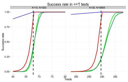
Figure 1: Plot of success probability of Hwang’s group testing algorithms for $(K,N)=(10,500)$ and $(30,9699)$. The simulated success probability of the HGBSA is plotted as a bright green line, and the related algorithm analysed in Section IV is plotted in dark green. The upper bound on success probability of Theorem III.1 is plotted in red, and the upper bound of [9] Equation (6) in blue. The dotted vertical line is at $\log_{2}\binom{N}{K}$.

IV A tighter upper bound

We now give a tighter upper bound on the performance of the HGBSA by controlling the size of the samples to be binary-searched, aiming to make the probability of observing a negative test slightly less than 1/2. This algorithm offers performance similar to the HGBSA, but reduces the gap between the bounds of Theorem II.3 and Theorem III.1 from $K$ to under $K/2$.

We briefly illustrate the performance of these algorithms by simulation. In the two cases of Figure 1 we keep the parameter $\beta=0.63$ fixed and plot the success probability of the algorithms compared with the lower bound of Theorem III.1 for different problem sizes.

We now describe the algorithm to prove Theorem IV.3. We group the tests in $K$ rounds, each of which comprises a sequence of negative tests before a positive test. Once a positive test occurs, we can find a defective using binary search as in Lemma II.1. We introduce the following notation, which allows us to keep track of the size of each subproblem (round).

Definition IV.1

We refer to an item which has not yet appeared in a negative test as a Possible Defective. We write $N^{(i)}_{j}$ the number of Possible Defectives left after the $j$-th consecutive negative test of the $i$-th round and $N^{(i)}_{0}$ for the number of Possible Defectives at the start of the $i$-th round, and write $K^{(i)}=K-i+1$ for the number of defectives in the $i$-th round. We write ${S}^{(i)}_{j}$ for the indicator that the $j$-th test of the $i$-th round is positive. Finally define $T_{i}$ as the random time of the last negative test of the round.

After every negative test the set of Possible Defectives will be reduced. In particular, if we denote by ${b}^{(i)}_{j}$ the size of the $j$-th test in the $i$-th round, then

$${N}^{(i)}_{j+1}={N}^{(i)}_{j}-{b}^{(i)}_{j+1},\ 1\leq i\leq K,\ 0\leq j\leq T_{i}\ .$$ (9)

As described previously, we use maximally informative tests by making the probability of observing a negative test (just) less than $1/2$. By truncating binomial coefficients, we prove:

Lemma IV.2

Conditional on having observed $j-1$ consecutive negative tests in the $i$-th round of Hwang’s algorithm, any random sample of size

$${b}^{(i)}_{j}\leq{N}^{(i)}_{j-1}\left(1-2^{-1/{K}^{(i)}}\right)-({K}^{(i)}-1)\ .$$ (10)

has probability less than $1/2$ of being negative, that is

$${\mathbb{P}}({S}^{(i)}_{j}=0\mid{S}^{(i)}_{0}=0,\ldots,{S}^{(i)}_{j-1}=0)\leq 1/2.$$

If the test is negative, we update ${N}^{(i)}_{j}$ using (9). If the test is positive, the only upper bound we can derive for sure for the new size of the set of possible defectives is ${N}^{(i)}_{j}\leq{N}^{(i)}_{j-1}-1$, as we’re only sure that one (defective) item will be removed from the set. By induction, within each round the following formulae for ${b}^{(i)}_{j}$ and ${N}^{(i)}_{j}$ hold:

$${b}^{(i)}_{j}=2^{-\frac{j-1}{K^{(i)}}}\left[N(1-2^{-1/K^{(i)}})-(K^{(i)}-1)\right]$$ (11)

$${N}^{(i)}_{j}=2^{-\frac{j}{K^{(i)}}}{N}^{(i)}_{0}+(K^{(i)}-1)\sum_{h=0}^{j-1}2^{-\frac{h}{K^{(i)}}}\ .$$ (12)

Here ${N}^{(i)}_{0}$ clearly depends on the previous round; it equals $N$ for $i=1$ and it can be suitably upper bounded for $i\geq 2$. With these results we can produce an upper bound on the average number of tests for this version of Hwang’s algorithm.

Theorem IV.3

Our version of Hwang’s algorithm is guaranteed to succeed with number of tests satisfying:

$$T_{tot}\leq K\log N+(1+\log\ln 2)K-\log K!+R\ .$$ (13)

where $R$ is a negative random term.

Proof:

We observe that

$${b}^{(i)}_{j}=\left\lceil{N}^{(i)}_{j-1}\left(1-2^{-1/{K}^{(i)}}\right)\right\rceil\leq 2{N}^{(i)}_{j-1}\left(1-2^{-1/{K}^{(i)}}\right)\ .$$ (14)

Similarly, repeatedly substituting (10) in (9) we obtain

$${N}^{(i)}_{j}\leq{N}^{(i)}_{0}2^{-j/{K}^{(i)}}\ .$$ (15)

This can be plugged back into (14), giving

$${b}^{(i)}_{j}\leq 2{N}^{(i)}_{0}2^{-(j-1)/{K}^{(i)}}(1-2^{-1/{K}^{(i)}})\ .$$ (16)

We can then compute the upper bound on the total number of tests using Lemma II.1. The number of tests in the $i$th round satisfies:

$$T_{tot}^{(i)}=T_{i}+\log{b}^{(i)}_{T_{i}+1}\leq T_{i}+1+\log{N}^{(i)}_{0}$$

$$-\displaystyle{\frac{T_{i}}{{K}^{(i)}}}+\log(1-2^{-1/{K}^{(i)}})\ .$$ (17)

In order to obtain a bound on the total number of tests we have to relate ${N}^{(i)}_{0}$ with ${N}^{(i-1)}_{T_{i-1}}$. Recalling Lemma II.1, we define $L_{i}$ by making $1+L_{i}$ be the position of the leftmost defective in the $(T_{i}+1)$-th sample, thus obtaining the equality

$${N}^{(i+1)}_{0}={N}^{(i)}_{T_{i}}-L_{i}\ .$$ (18)

Using iteratively the update formulae ${N}^{(i)}_{j}\leq{N}^{(i)}_{0}2^{-j/{K}^{(i)}}$ and (18), we can deduce that $\log{N}^{(i+1)}_{0}$ equals

$$\log N-\sum_{j=1}^{i}\displaystyle{\frac{T_{j}}{{K}^{(j)}}}+\log\left[1-\displaystyle{\frac{1}{N}}\sum_{h=1}^{i}\displaystyle{\frac{L_{h}}{\prod_{j=1}^{h}2^{-T_{j}/{K}^{(j)}}}}\right]\ .$$

Summing together the bounds for the number of tests in each round, calling $C_{i}$ the last addend above and $R=\sum_{i=1}^{n}C_{i}$:

$$T_{tot} \leq K\log N+K+\sum_{i=1}^{K}\log(1-2^{-1/{K}^{(i)}})+R.$$ (19)

To gain a more manageable expression, we bound the penultimate term of (19). Calling $f(x):=2^{-x}-1+x\ln 2$, notice that $f^{\prime}(x)\geq 0$ for $x\geq 0$ and $f(0)=0$; in particular, $1-2^{-1/i}\leq\displaystyle{\frac{1}{i}}\ln 2$. Substituting ${K}^{(i)}=K-i+1$, reversing the order of the sum and taking logs, we deduce the result. ∎

It is hard to say more about the random terms $C_{i}$ than that they are negative, though we hope that future simulation and probabilistic bounds will give us further insights into the resulting number of tests required. Notice the slightly suprising feature that the number of negative tests $T_{i}$ has no effect on the final bound (19). This can be explained by the fact that summing (17) over $i$ creates a double sum over $i$ and $j$, and that the coefficients of $T_{i}$ exactly cancel.

V Conclusion

Using a sharper information-theoretic lower bound, we have shown that in the noiseless adaptive case, the capacity of group testing is 1, and that for an erasure channel, the capacity is $1-p$. For other noise models, we have found lower bounds on the capacity. It remains of interest to find exact values of the capacity in other cases, including non-adaptive problems.

References

- [1] R. Dorfman, “The detection of defective members of large populations,” The Annals of Mathematical Statistics, pp. 436–440, 1943.
- [2] Y. Erlich, A. Gordon, M. Brand, G. Hannon, and P. Mitra, “Compressed genotyping,” IEEE Trans. Inform. Theory, vol. 56, no. 2, pp. 706–723, 2010.
- [3] N. Shental, A. Amir, and O. Zuk, “Identification of rare alleles and their carriers using compressed se (que) nsing,” Nucleic acids research, vol. 38, no. 19, pp. e179–e179, 2010.
- [4] C. Aksoylar, G. Atia, V. Saligrama, “Sparse Signal Processing with Linear and Non-Linear Observations: A Unified Shannon Theoretic Approach,” arXiv:1304.0682
- [5] M. Malyutov, “Search for sparse active inputs: a review,” in H. Aydinian, F. Cicalese, C. Deppe (ed.), Information Theory, Combinatorics and Search Theory, Lecture Notes in Computer Science, Springer, London, 2013.
- [6] M. Malyutov, “Mathematical models and results in the theory of screening experiments”, in M. Malyutov (ed.), Theoretical Problems of Experimental Design, Soviet Radio, Moscow, pp. 5-69, 1977.
- [7] G. Atia, S. Aeron, E. Ermis, and V. Saligrama, “On throughput maximization and interference avoidance in cognitive radios,” in 5th IEEE Consumer Communications and Networking Conference, 2008. IEEE, 2008, pp. 963–967.
- [8] G. Atia and V. Saligrama, “Boolean compressed sensing and noisy group testing,” IEEE Trans. Inform. Theory, vol. 58, no. 3, pp. 1880 –1901, March 2012.
- [9] C. L. Chan, P. H. Che, S. Jaggi, and V. Saligrama, “Non-adaptive probabilistic group testing with noisy measurements: Near-optimal bounds with efficient algorithms,” in 49th Allerton Conference, Sept. 2011, pp. 1832 –1839.
- [10] J. Haupt, R. Castro, and R. Nowak, “Distilled sensing: Adaptive sampling for sparse detection and estimation,” IEEE Trans. Inform. Theory, vol. 57, no. 9, pp. 6222 –6235, Sept. 2011.
- [11] M. Aldridge, “Adaptive group testing as channel coding with feedback,” in 2012 IEEE International Symposium on Information Theory (ISIT) Proceedings,, July 2012, pp. 1832 –1836.
- [12] C. E. Shannon, “A mathematical theory of communication,” Bell System Tech. J., vol. 27, pp. 379–423, 623–656, 1948.
- [13] D. Donoho and J. Jin, “Higher criticism for detecting sparse heterogeneous mixtures,” Ann. Statist., vol. 32, no. 3, pp. 962–994, 2004.
- [14] J. H. B. Kemperman, “Strong converses for a general memoryless channel with feedback,” in Trans. 6th Prague Conf. on Information Theory, Stat. Dec. Fcts and Rand. Proc., 1973.
- [15] D. Du and F. Hwang, Combinatorial Group Testing and Its Applications, ser. Series on Applied Mathematics. World Scientific, 1993.
- [16] T. Wadayama, “An Analysis on Non-Adaptive Group Testing based on Sparse Pooling Graphs,” 2013 IEEE International Symposium on Information Theory (ISIT) Proceedings, July 2013
- [17] M. P. Aldridge, L. Baldassini, and O. T. Johnson, “Group testing algorithms: bounds and simulations,” in preparation.
- [18] F. K. Hwang, “A method for detecting all defective members in a population by group testing,” Journal of the American Statistical Association, vol. 67, no. 339, pp. 605–608, 1972.