Classification of the solutions to an overdetermined elliptic problem in the plane

March 22, 2013

Abstract: we classify the solutions to an overdetermined elliptic problem in the plane in the finite connectivity case. This is achieved by establishing a one-to-one correspondence between the solutions to this problem and a certain type of minimal surfaces.

1. Introduction

In the theory of elliptic P.D.E., an overdetermined problem is one where both the Dirichlet and Neumann boundary values are prescribed. This puts strong geometric constraints on the domain. For example, a famous result of J. Serrin [25] asserts that if $\Omega$ is a bounded domain in ${\mathbb{R}}^{n}$ which admits a function $u$ solution of $\Delta u=-1$ in $\Omega$ with Dirichlet boundary value $u=0$ on $\partial\Omega$ and Neumann boundary value $\frac{\partial u}{\partial\nu}$ constant on $\partial\Omega$, then $\Omega$ is a ball. Overdetermined elliptic problems appear in various mathematical and physical problems, such as isoperimetric inequalities, spectral geometry and hydrodynamics. (See for example the survey [3].)

In [14], F. Hélein, L. Hauswirth and F. Pacard have proposed the following overdetermined problem. Let $\Omega$ be a smooth, unbounded domain in ${\mathbb{R}}^{n}$ with non-empty boundary. The domain $\Omega$ is called exceptional if it admits a positive harmonic function $u$ which has Dirichlet boundary value $u=0$ on $\partial\Omega$ and Neumann boundary value $\frac{\partial u}{\partial\nu}=c$ on $\partial\Omega$, where $c$ is a constant. By the boundary maximum principle, the constant $c$ must be negative, and we may normalize $c=-1$ by scaling of $u$. Also, when $u$ is constant on $\partial\Omega$, the Neumann boudary condition is equivalent to $|\nabla u|=|c|$ on $\partial\Omega$. So we may formulate the above problem as:

(1) $$\left\{\begin{array}[]{ll}\Delta u=0&\mbox{ in $\Omega$,}\\ u>0&\mbox{ in $\Omega$,}\\ u=0&\mbox{ on $\partial\Omega$,}\\ |\nabla u|=1&\mbox{ on $\partial\Omega$}.\end{array}\right.$$

This problem is related to the study of extremal domains, namely domains $\Omega$ in a Riemannian manifold which are critical points for the functional $\lambda_{1}(\Omega)$ under a volume constraint, where $\lambda_{1}$ denotes the first eigenvalue of the Laplace Beltrami operator. See [14] for more details.

For example, a half-space or the complementary of a ball are exceptional domains. In [14], the authors discovered that in the case $n=2$, the domain $|y|<\frac{\pi}{2}+\cosh x$ in the plane is an exceptional domain. They also developed a Weierstrass type Representation for exceptional domains in the plane that are simply connected, and noted a strong analogy with minimal surfaces. In this paper, we prove that the analogy goes very deep by establishing a one-to-one correspondence between exceptional domains and a certain type of minimal surfaces which we call minimal bigraphs. This correspondence allows us to find examples and classify solutions.

We only address Problem (1) in the case of planar domains ($n=2$) and we identify ${\mathbb{R}}^{2}$ with the complex plane ${\mathbb{C}}$. The assumption that $\Omega$ is a smooth domain can be relaxed (see Proposition 1). Also, the solution $u$ of Problem (1), when it exists, is unique (see Proposition 2).

By a trivial exceptional domain, we mean a half-plane. Let $\Omega$ be a non-trivial exceptional domain. In Section 3, we use the theory of univalent functions to prove that

• If $\Omega$ has finite connectivity, then $|\nabla u|<1$ in $\Omega$.

• If $\Omega$ is periodic and has finite connectivity in the quotient, then $|\nabla u|<1$ in $\Omega$.

By finite connectivity, we mean that $\partial\Omega$ has a finite number of components. By periodic, we mean that $\Omega$ is invariant by a non-zero translation $T$. Note that an exceptional domain cannot be doubly periodic (for the maximum principle implies that $u\equiv 0$ in this case).

In Sections 4, 5 and 6, we establish a one-to-one correspondence between the following two classes of objects:

• exceptional domains $\Omega$ such that $|\nabla u|<1$ in $\Omega$,

• complete, embedded minimal surfaces $M$ in ${\mathbb{R}}^{3}$ which are symmetric with respect to the horizontal plane $x_{3}=0$ and such that $M^{+}=M\cap\{x_{3}>0\}$ is a graph over the unbounded domain in the plane bounded by $M\cap\{x_{3}=0\}$. We call such a minimal surface a minimal bigraph.

(In fact, we will establish the above correspondence assuming that the domain $\Omega$ satisfies a mild additional geometric hypothesis, namely that its complement in non-thinning: see Definition 1. This hypothesis is always satisfied for domains with finite connectivity, or periodic domains with finite connectivity in the quotient). For example:

1. The vertical catenoid is a minimal bigraph. It corresponds to the exceptional domain $\Omega={\mathbb{C}}\setminus D(0,1)$.

2. The horizontal catenoid is a minimal bigraph. It corresponds to the exceptional domain $|y|<\frac{\pi}{2}+\cosh x$ discovered in [14].

3. Scherk’s family of simply periodic minimal surfaces, suitably rotated, are minimal bigraphs. They correspond to a new family of periodic exceptional domains. (In fact, this family was already known! See Section 1.1.)

We give more details about these examples in Section 7.

In Section 8, we take advantage of the correspondence to translate classification results from minimal surface theory into classification results for exceptional domains. We prove that (up to similitude)

• The only exceptional domains in the plane with finite connectivity are the half-plane and Examples (1) and (2),

• The only periodic exceptional domains with finite connectivity in the quotient are the half-plane and Examples (3).

Finally, in Section 9, we extend the correspondence to the case of immersed domains in the plane.

1.1. Related works

Laurent Hauswirth pointed out to me that Problem (1) has been studied by D. Khavinson, E. Lundberg and R. Teodorescu in a recent paper [16]. They obtain classification results in the $2$-dimensional case under stronger topological hypotheses than ours. They prove that if an exceptional domain $\Omega$ is the complement of a bounded domain, then it is the complement of a disk; if it is simply-connected and Smirnov, then it is a half-plane or the domain $|y|<\frac{\pi}{2}+\cosh x$, up to similitude. In the simply-connected case, their results are stronger than ours because they do not assume that the boundary of $\Omega$ has a finite number of components. They also prove that in higher dimension, an exceptional domain in ${\mathbb{R}}^{n}$ whose complement is bounded, connected and has $C^{2,\alpha}$ boundary, is the exterior of a sphere.

I learned from Erik Lundberg that the family of periodic exceptional domains (the ones corresponding to Scherk surfaces) already appears in a 1976 paper by G. R. Baker, P. G. Saffman and J. S. Sheffield [2] as a solution to an equilibrium problem in hydrodynamics. It is also discussed by D. Crowdy and C. Green in [6].

Several authors have studied the following, more general overdetermined elliptic problem

(2) $$\left\{\begin{array}[]{ll}\Delta u=f(u)&\mbox{ in $\Omega$}\\ u>0&\mbox{ in $\Omega$}\\ u=0&\mbox{ on $\partial\Omega$}\\ \frac{\partial u}{\partial\nu}=c&\mbox{ on $\partial\Omega$}\end{array}\right.$$

where $\Omega$ is a domain in ${\mathbb{R}}^{n}$ and $f$ is some given function. A formal analogy between this kind of problem and constant mean curvature (CMC) hypersurfaces in ${\mathbb{R}}^{n+1}$ has been observed. For example, the quoted result of J. Serrin [25] is the counterpart of the theorem of A.D. Alexandrov, which asserts that the only embedded compact CMC hypersurfaces in ${\mathbb{R}}^{n+1}$ are round spheres. In [26], F. Schlenk and P. Sicbaldi have constructed solutions to Problem (2) in the case $f(x)=\lambda x$, which are analogues of the Delaunay CMC surfaces in ${\mathbb{R}}^{3}$. In the case $n=2$, the analogy between Problem (2) and CMC surfaces has been explored in a systematic way by A. Ros and P. Sicbaldi in a very interesting paper [22]. See the first section of this paper for more results in this spirit and related conjectures.

2. Preliminary remarks

The assumption that $\Omega$ is a smooth domain can be relaxed. Recall ([11] page 94) that an open set $\Omega$ in ${\mathbb{R}}^{n}$ with non-empty boundary is a domain of class $C^{k}$ (resp. smooth, analytic…) if for each point $x_{0}\in\partial\Omega$, there exists $\varepsilon>0$ and a diffeomorphisme $\psi$ of class $C^{k}$ (resp. smooth, analytic…) from the ball $B(x_{0},\varepsilon)$ to a domain $D\subset{\mathbb{R}}^{n}$ such that

$$\psi(B(x_{0},\varepsilon)\cap\Omega)=D\cap{\mathbb{R}}^{n}_{+},\qquad\psi(B(x_{0},\varepsilon)\cap\partial\Omega)=D\cap\partial{\mathbb{R}}^{n}_{+}$$

where ${\mathbb{R}}^{n}_{+}$ is the upper half space $x_{n}>0$. (If $k=0$, then diffeomorphism of class $C^{0}$ means homeomorphism.)

Proposition 1.

Let $\Omega$ be a domain of class $C^{0}$ in the plane. Assume that Problem (1) has a “classical” solution $u$, namely: $u$ is of class $C^{2}$ in $\Omega$, $\Delta u=0$, $u>0$ in $\Omega$, and

$$\forall z_{0}\in\partial\Omega,\quad\lim_{z\to z_{0}}u(z)=0\quad\mbox{ and }\lim_{z\to z_{0}}|\nabla u(z)|=1.$$

Then $\Omega$ is a smooth domain (actually, real analytic). Moreover, $u$ extends to a harmonic function defined in a neighborhood of $\Omega$.

Proof: Let $z_{0}\in\partial\Omega$. By the definition of a domain of class $C^{0}$, $z_{0}$ has a neighborhood $V_{z_{0}}$ such that $V_{z_{0}}\cap\Omega$ is a Jordan domain (meaning that its boundary is a Jordan curve). Let $f:D^{+}(0,1)\to V_{z_{0}}\cap\Omega$ be a conformal representation on the upper half-disk. Then $f$ extends to a homeomorphism of the closure of $D^{+}(0,1)$ to the closure of $V_{z_{0}}\cap\Omega$ by Caratheodory’s theorem (Theorem 13.2.3 in [13]). We may choose $f$ so that $f$ maps $(-1,1)$ to $V_{z_{0}}\cap\partial\Omega$. Consider the harmonic function ${\widetilde{u}}(z)=u\circ f(z)$ on $D^{+}(0,1)$. Then ${\widetilde{u}}$ is the real part of a holomorphic function $U$ on $D^{+}(0,1)$. Moreover,

$$\forall x_{0}\in(-1,1),\quad\lim_{z\to x_{0}}{\rm Re}\,U(z)=0$$

so $U$ extends to a holomorphic function on $D(0,1)$ by the Schwarz reflection principle. On the other hand, $U^{\prime}=2{\widetilde{u}}_{z}$ gives

$$\frac{U^{\prime}(z)}{f^{\prime}(z)}=2u_{z}(f(z))\quad\mbox{ for $z\in D^{+}(0,1)$}.$$

Of course, we do not know yet that $f^{\prime}$ extends continuously to $(-1,1)$. But our hypothesis on $u$ tells us that the ratio $|\frac{U^{\prime}(z)}{f^{\prime}(z)}|$ does, and morevoer,

$$\forall x_{0}\in(-1,1),\quad\lim_{z\to x_{0}}\left|\frac{U^{\prime}(z)}{f^{\prime}(z)}\right|=1.$$

Consequently, there exists $\varepsilon_{1}>0$ such that $\frac{U^{\prime}(z)}{f^{\prime}(z)}\neq 0$ for $z\in D^{+}(0,\varepsilon_{1})$. Consider the holomorphic function $h(z)=\log\frac{U^{\prime}(z)}{f^{\prime}(z)}$ on $D^{+}(0,\varepsilon_{1})$. Then $\lim_{z\to x_{0}}{\rm Re}\,h(z)=0$ for $x_{0}\in(-\varepsilon_{1},\varepsilon_{1})$, so $h$ extends to a holomorphic function in the disk $D(0,\varepsilon_{1})$. Hence $f^{\prime}$ and $f$ extends holomorphically to the disk $D(0,\varepsilon_{1})$, and $f^{\prime}\neq 0$ in this disk, so $f$ is biholomorphic in a disk $D(0,\varepsilon_{2})$. This implies that the boundary of $\Omega$ is real analytic in a neighborhood of $z_{0}$. Moreover, the formula $u(z)={\rm Re}\,U(f^{-1}(z))$ shows that $u$ can be extended to a function harmonic in a neighborhood of $z_{0}$. The extension is unique by analyticity so this shows that $u$ can be extended to a neighborhood of $\Omega$. $\Box$

Remark 1.

A similar regularity result is obtained by D. Khavinson, E. Lundberg and R. Teodorescu in [16], Corollary 2.3, assuming that $\Omega$ is of class $C^{2}$.

Proposition 2.

Let $\Omega$ be an exceptional domain. Then Problem (1) has a unique solution $u$.

Proof: Let $u^{\prime}$ be another solution. Then the difference $v=u-u^{\prime}$ satisfies $\Delta v=0$ in $\Omega$ and $v=dv=0$ on $\partial\Omega$. By Proposition 1, both $u$ and $u^{\prime}$ extend to a neighborhood of $\Omega$. Then the function $v_{z}$ is holomorphic in a neighborhood of $\Omega$ and $v_{z}=0$ on $\partial\Omega$ so the zeros of $v_{z}$ are not isolated. Hence $v_{z}\equiv 0$ and $v\equiv 0$ in $\Omega$. $\Box$

Proposition 3.

Let $\Omega$ be a smooth domain in the plane. Then each component of $\partial\Omega$ is either a smooth Jordan curve or the image of a smooth proper embedding $\gamma:{\mathbb{R}}\to{\mathbb{C}}$ (where proper means $\lim_{t\to\pm\infty}\gamma(t)=\infty$). We call the later a proper arc.

Proof. Each component of $\partial\Omega$ is a 1-dimensional submanifold so is either diffeomorphic to the circle ${\mathbb{S}}^{1}$ or the real line. In the first case, it is a smooth Jordan curve. In the later case, it is the image of an embedding $\gamma:{\mathbb{R}}\to{\mathbb{C}}$. We claim that $\gamma$ is proper. If not, then there exists a sequence $t_{n}\to\pm\infty$ such that $\gamma(t_{n})$ has a finite limit $p$. Now $p$ must be on the boundary of $\Omega$. The definition of a smooth domain at $p$ gives a contradiction. $\Box$

The condition $|\nabla u|<1$, which we will address in Section 3, has the following interesting geometric consequence for the domain $\Omega$:

Proposition 4.

Let $\Omega$ be an exceptional domain such that $|\nabla u|<1$. Then $\Omega$ is a strictly concave domain, namely: each component of ${\mathbb{C}}\setminus\Omega$ is strictly convex.

Proof. The curvature of the level set $u=0$ is given by ([12] page 72)

(3) $$\kappa=\frac{u_{xx}u_{y}^{2}+u_{yy}u_{x}^{2}-2u_{xy}u_{x}u_{y}}{(u_{x}^{2}+u_{y}^{2})^{3/2}}.$$

Regarding sign, the curvature is positive when the curvature vector points toward $u<0$ (as can be checked in the case $u(x,y)=x^{2}+y^{2}-1$: Formula (3) gives $\kappa=1$). Consider the harmonic function $g(z)=-\log|2u_{z}(z)|$. Then $g=0$ on $\partial\Omega$ and $g>0$ in $\Omega$. Let $z_{0}\in\partial\Omega$. By rotation we may assume that $z_{0}=0$ and $\nabla u(0)=(1,0)$. Then for small $\varepsilon>0$, $(0,\varepsilon)\subset\Omega$. By the boundary maximum principle (Lemma 3.4. in [11]), $g_{x}(0)>0$. On the other hand,

$$g_{x}(0)=-\frac{1}{|\nabla u(0)|^{2}}(u_{x}(0)u_{xx}(0)+u_{y}(0)u_{xy}(0))=-u_{xx}(0).$$

Hence $u_{xx}(0)<0$. Since $u$ is harmonic we obtain $u_{yy}(0)>0$. Formula (3) gives $\kappa(0)>0$. This means that the curvature vector of the boundary points outside of $\Omega$, so the boundary is locally strictly concave. Each component of $\partial\Omega$ is then globally a strictly convex curve, meaning that it bounds a strictly convex subset of the plane. (For the components of $\partial\Omega$ which are Jordan curves, this is standard. For the components of $\partial\Omega$ which are proper arcs, this is also true, see Theorem 9.40 in [20].) $\Box$

Let $C$ be a convex set in the plane. For $\varepsilon>0$, we define

$$\mu_{\varepsilon}(C)=\inf_{p\in C}\mbox{\rm Area}(C\cap D(p,\varepsilon)).$$

If $C$ is a convex set with non-empty interior then $\mu_{\varepsilon}(C)>0$.

Definition 1.

Consider a subset $A$ of the plane which is the union of a family of disjoint convex sets $(C_{i})_{i\in I}$. We say that $A$ is non-thinning if for some $\varepsilon>0$ we have

$$\inf_{i\in I}\mu_{\varepsilon}(C_{i})>0.$$

We will establish the correspondence in the case where the complement of $\Omega$ is non-thinning. This prevents the components of ${\mathbb{C}}\setminus\Omega$ from becoming thinner and thinner. Clearly if $\Omega$ is a concave domain with finite connectivity, or a concave periodic domain with finite connectivity in the quotient, then its complement is non-thinning.

3. The condition $|\nabla u|<1$.

The goal of this section if to prove the following theorem.

Theorem 1.

Let $\Omega$ be a non-trivial exceptional domain with finite connectivity (which means that $\partial\Omega$ has a finite number of components). Then $|\nabla u|<1$ in $\Omega$.

We will in fact get more precise results: see Theorems 2, 5 and 6. We will also prove a result in the periodic case: see Theorem 7.

3.1. The case $\partial\Omega$ compact

We start with the case where $\partial\Omega$ is the union of a finite number of Jordan curves.

Theorem 2.

Let $\Omega$ be an exceptional domain such that ${\mathbb{C}}\setminus\Omega$ is bounded. Then $|\nabla u|<1$ in $\Omega$ and

$$\lim_{|z|\to\infty}\nabla u(z)=0.$$

Proof. Let ${\widetilde{u}}(z)=u(\frac{1}{z})$. Then ${\widetilde{u}}$ is a positive harmonic function in a punctured disk $D^{*}(0,\varepsilon)$. By Bôcher Theorem (Theorem 3.9 in [1]), we can write

$${\widetilde{u}}(z)=c\log|z|+h(z)$$

where $c$ is a constant and $h$ is harmonic in the disk $D(0,\varepsilon)$. Then

$$u(z)=-c\log|z|+h(\frac{1}{z}),$$

$$u_{z}(z)=-\frac{c}{2z}-h_{z}(\frac{1}{z})\frac{1}{z^{2}}.$$

Hence there exists $R$ such that $|\nabla u|<1$ for $|z|\geq R$. Then we have $|\nabla u|\leq 1$ on the boundary of $\Omega\cap D(0,R)$. By the maximum principle, we have $|\nabla u|\leq 1$ in $\Omega\cap D(0,R)$. Moreover, $u_{z}$ is not constant in $\Omega$ so the maximum principle implies that $|\nabla u|<1$ in $\Omega$. $\Box$

Remark 2.

D. Khavinson, E. Lundberg and R. Teodorescu ([16], Theorem 3.2) have proved that under the hypothesis of Theorem 2, $\Omega$ is the complement of a disk, which implies the conclusion of the theorem.

3.2. A Phragmen Lindelöf type result for univalent functions in the upper half-plane

Next we would like to do the case where $\partial\Omega$ is a proper arc. For this we need a result about univalent function in the upper half-plane ${\rm Im}\,z>0$, which we denote $H$. (Recall that univalent means holomorphic injective.) We have the following distortion theorem for univalent functions in the half-plane, which is an easy consequence of the standard distortion theorem for univalent functions in the disk:

Theorem 3.

Let $f$ be univalent in the upper half-plane $H$ and normalized by $f(i)=0$ and $f^{\prime}(i)=1$. Then for $z\in H$,

$$4\frac{|z+i|-|z-i|}{(|z+i|+|z-i|)^{3}}\leq|f^{\prime}(z)|\leq 4\frac{|z+i|+|z-i|}{(|z+i|-|z-i|)^{3}}.$$

Proof: Consider the Möbius transformation

(4) $$w=\varphi(z)=\frac{z-i}{iz-1}$$

This transformation is involutive and exchanges the upper half-plane $H$ with the unit disk $D(0,1)$. Consider the function $F$ defined in the disk by $f(z)=-2F(\varphi(z))$. Taking the derivative,

(5) $$f^{\prime}(z)=\frac{4}{(iz-1)^{2}}F^{\prime}(\varphi(z)).$$

So the function $F$ is univalent in the disk and satisfies $F(0)=0$, $F^{\prime}(0)=1$. The distortion theorem for normalized univalent functions in the disk (Theorem 2.5 in [8]) tells us that

(6) $$\frac{1-|w|}{(1+|w|)^{3}}\leq|F^{\prime}(w)|\leq\frac{1+|w|}{(1-|w|)^{3}},\quad\mbox{ $w\in D$.}$$

The result follows by substitution in (5). $\Box$

Using this theorem, we prove the following:

Theorem 4.

Let $f$ be an univalent function in the upper half-plane $H$ that extends $C^{1}$ to $\overline{H}$. Let $c$ be a positive number.

1. If $|f^{\prime}|\leq c$ on $\partial H$ then $|f^{\prime}|\leq c$ in $H$.

2. If $|f^{\prime}|\geq c$ on $\partial H$ then $|f^{\prime}|\geq c$ in $H$.

3. If $|f^{\prime}|$ is constant on $\partial H$ then $f^{\prime}$ is constant in $H$.

Proof: Without loss of generality, we may assume (replacing $f$ by $af+b$) that $f(i)=0$ and $f^{\prime}(i)=1$. Theorem 3 gives

$$4\frac{|z+i|^{2}-|z-i|^{2}}{(|z+i|+|z-i|)^{4}}\leq|f^{\prime}(z)|\leq 4\frac{(|z+i|+|z-i|)^{4}}{(|z+i|^{2}-|z-i|^{2})^{3}}.$$

which implies, with $z=x+iy$

(7) $$\frac{y}{(|z|+1)^{4}}\leq|f^{\prime}(z)|\leq\frac{(|z|+1)^{4}}{y^{3}}.$$

The first two points of the theorem follow from Lemma 1 below (with $g=f^{\prime}$ in the first case and $g=1/f^{\prime}$ in the second one). To prove the third point, assume that $|f^{\prime}|\equiv c$ on $\partial H$. By the first two points, $|f^{\prime}|\equiv c$ in $H$. Since $f^{\prime}$ is holomorphic, it must be constant in $H$. $\Box$

Lemma 1.

Let $g$ be a holomorphic function on the upper half-plane $H$, continuous on $\overline{H}$. Assume that

$$|g(z)|\leq c_{1}\frac{(|z|+1)^{n}}{y^{m}}\quad\mbox{ in $H$,}$$

$$|g(z)|\leq c_{2}\quad\mbox{ on $\partial H$}$$

for some positive numbers $c_{1},c_{2}$ and positive integers $n,m$. Then $|g(z)|\leq c_{2}$ in $H$.

Proof: We prove that $|g(z)|$ has polynomial growth and conclude with the Phragmen Lindelöf principle. Given $R\geq 1$, consider the rectangular domain $\Omega_{R}=(-R,R)\times(0,1)$ and the function

$$h_{R}(z)=(z-R)^{m}(z+R)^{m}.$$

We estimate the function $g(z)h_{R}(z)$ on $\partial\Omega_{R}$. On $\{\pm R\}\times(0,1)$, we have

$$|g(z)|\leq c_{1}\frac{(R+2)^{n}}{y^{m}},\quad|h_{R}(z)|\leq y^{m}(2R+1)^{m}\quad\Rightarrow|g(z)h_{R}(z)|\leq CR^{m+n}$$

where the letter $C$ means a constant independant of $z$ and $R$. On $[-R,R]\times\{0\}$, we have

$$|g(z)|\leq c_{2},\quad|h_{R}(z)|\leq R^{2m}\quad\Rightarrow|g(z)h_{R}(z)|\leq c_{2}R^{2m}.$$

On $[-R,R]\times\{1\}$, we have

$$|g(z)|\leq c_{1}(R+2)^{n},\quad|h_{R}(z)|\leq(2R+1)^{2m}\quad\Rightarrow|g(z)h_{R}(z)|\leq CR^{2m+n}.$$

Hence $|g(z)h_{R}(z)|\leq CR^{2m+n}$ on $\partial\Omega_{R}$. By the maximum principle, $|g(z)h_{R}(z)|\leq CR^{2m+n}$ in $\Omega_{R}$. Now if $|x|\leq\frac{R}{2}$, we have $|h_{R}(z)|\geq(\frac{R}{2})^{2m}$, hence

$$|g(z)|\leq CR^{n}.$$

This implies that in the band ${\mathbb{R}}\times[0,1]$,

(8) $$|g(z)|\leq C(|z|+1)^{n}.$$

For $y\geq 1$, (8) is true by the first hypothesis on $g$. Hence (8) holds in the whole upper half-plane. By the Phragmen Lindelöf principle for the half-plane (Corollary 4.2 in [4]), $|g(z)|\leq c_{2}$ in $H$. $\Box$

3.3. The case where $\partial\Omega$ is a proper arc

Theorem 5.

Let $\Omega$ be an exceptional domain such that $\partial\Omega$ is a proper arc. Then $|\nabla u|=1$ in $\Omega$ and $\Omega$ is a half-plane.

Proof. Let $\gamma:{\mathbb{R}}\to{\mathbb{C}}$ be a parametrization of $\partial\Omega$. Since $\gamma$ is proper, it extends to a continuous, injective map from the extended real line ${\mathbb{R}}\cup\{\infty\}\simeq{\mathbb{S}}^{1}$ to the Riemann sphere ${\mathbb{C}}\cup\{\infty\}$. Hence $\Omega$ is bounded in the Riemann sphere by a Jordan curve. By the Riemann mapping theorem, there exists a conformal representation $F$ from the unit disk $D(0,1)$ to $\Omega$. By Caratheodory’s Theorem (Theorem 13.2.3 in [13]), $F$ extends to a homeomorphism from the closed disk $\overline{D}(0,1)$ to the closure of $\Omega$ in the Riemann sphere, namely, $\overline{\Omega}\cup\{\infty\}$. Without loss of generality, we may assume that $F(-i)=\infty$. Composing with the Moebius map $\varphi$ defined in (4), we obtain a homeomorphism $f:\overline{H}\cup\{\infty\}\to\overline{\Omega}\cup\{\infty\}$ that is conformal in the upper half-plane $H$ and maps $\infty$ to $\infty$. Moreover, $f({\mathbb{R}})=\partial\Omega$. Since $\partial\Omega$ is smooth, $f$ extends $C^{1}$ to ${\mathbb{R}}$. (At this point, we know nothing about the regularity of $f$ at infinity.) Let ${\widetilde{u}}=u\circ f$. Then ${\widetilde{u}}$ is a positive harmonic function in $H$ with zero boundary value. By Theorem 7.22 in [1], ${\widetilde{u}}(z)=a\,{\rm Im}\,z$ for some positive constant $a$. Then

$${\widetilde{u}}_{z}(z)=u_{z}(f(z))f^{\prime}(z)=\frac{-ai}{2}$$

Since $|u_{z}|=1$ on $\partial\Omega$, we obtain that $|f^{\prime}|$ is constant on ${\mathbb{R}}$. By Theorem 4, $f^{\prime}$ is constant in $H$. This implies that $f$ is affine, so $\Omega$ is a half-plane, and $u_{z}$ is constant in $\Omega$. $\Box$

Remark 3.

F. Helein, L. Hauswirth and F. Pacard ([14], Proposition 6.1) have obtained this result under the additional hypothesis that $u_{x}>0$ in $\Omega$, a rather strong condition. D. Khavinson, E. Lundberg and R. Teodorescu ([16], Theorem 5.1) have also obtained this result under the hypothesis that $\Omega$ is a Smirnov domain.

3.4. The remaining case

Theorem 6.

Let $\Omega$ be a non-trivial exceptional domain of finite connectivity. Assume that $\partial\Omega$ is not bounded, so contains at least one proper arc. Then $|\nabla u|<1$ in $\Omega$. Moreover, for each end of $\Omega$, $\lim\nabla u(z)$ exists and its norm is equal to one. Finally, the number of proper arcs in $\partial\Omega$ is at most two.

Proof: Fix some large number $R$ such that:

• all Jordan curves in $\partial\Omega$ are contained in $D(0,R)$,

• all proper arcs in $\partial\Omega$ have at least one point in $D(0,R)$,

• $R$ is not a critical value of the function $|z|$ restricted to $\partial\Omega$.

The last point implies that $\partial\Omega$ is transverse to the circle $|z|=R$, so intersects this circle in a finite number of points. Consequently, $\partial\Omega\setminus D(0,R)$ has a finite number of components. Each such component is either a curve with two endpoints on the circle $C(0,R)$ or a proper arc with one endpoint. Consider an unbounded component $C$ of $\Omega\setminus D(0,R)$. By our choice of $R$, no component of $\partial C$ can be a component of $\partial\Omega$. Hence $\partial C$ has only one component, and we may decompose $\partial C$ as $\alpha_{1}\cdot\alpha_{2}\cdot\alpha_{3}$ where $\alpha_{1}$ and $\alpha_{3}$ are proper arcs $[0,\infty)\to{\mathbb{C}}$ with one endpoint on the circle $|z|=R$, both included in $\partial\Omega$, and $\alpha_{2}$ is a curve with two enpoints on $|z|=R$. (The curve $\alpha_{2}$ consists of arcs of the circle $|z|=R$ together with finite parts of $\partial\Omega$). Arguing as in the proof of Theorem 5, we can find a conformal representation $f:H\to C$ which extends to a homeomorphism from $\overline{H}\cup\{\infty\}$ to $\overline{C}\cup\{\infty\}$, mapping ${\mathbb{R}}$ to $\partial C$ and $\infty$ to $\infty$.

As in the proof of Theorem 5, let ${\widetilde{u}}=u\circ f$. Then ${\widetilde{u}}$ is a positive harmonic function in $H$. Since $H$ is simply connected, we may consider the conjugate harmonic function ${\widetilde{u}}^{*}$ of ${\widetilde{u}}$. Consider the holomorphic function

$$U(z):={\widetilde{u}}(z)+i{\widetilde{u}}^{*}(z),\quad z\in H.$$

Let $[a,b]=f^{-1}(\alpha_{2})$. Then ${\rm Re}\,U(z)=0$ on ${\mathbb{R}}\setminus[a,b]$. By the Schwarz reflection principle, $U$ extends to a holomorphic function on ${\mathbb{C}}\setminus[a,b]$. By the boundary maximum principle, since ${\widetilde{u}}>0$ in $H$, we have ${\widetilde{u}}_{y}>0$ on ${\mathbb{R}}\setminus[a,b]$. By the Cauchy Riemann equation, ${\widetilde{u}}^{*}_{x}=-{\widetilde{u}}_{y}$, so the function ${\widetilde{u}}^{*}$ is decreasing on $(-\infty,a)$ and $(b,\infty)$. Consequently, the function $U$ takes each pure imaginary value at most two times on ${\mathbb{C}}\setminus[a,b]$. By Picard’s theorem, $U$ has no essential singularity at $\infty$, so has at most a pole. Since ${\rm Re}\,U$ is positive in $H$, the pole has order at most one. This means that we can write

$$U(z)=-ciz+h(\frac{1}{z}),\quad z\in{\mathbb{C}}\setminus[a,b]$$

where the constant $c$ is non-negative and the function $h$ extends holomorphically at $0$. Then

$$U^{\prime}(z)=-ci-h^{\prime}(\frac{1}{z})\frac{1}{z^{2}}.$$

If $c=0$, let $m$ be the order of the zero of $h^{\prime}$ at $0$ (with $m=0$ if $h^{\prime}(0)\neq 0$). Then there are positive constants $c_{1}$ and $c_{2}$ such that

(9) $$\frac{c_{1}}{|z|^{m+2}}\leq|U^{\prime}(z)|\leq c_{2}\quad\mbox{ for $|z|$ large enough}.$$

If $c>0$, then (9) still holds with $m=-2$ and $c_{1}=\frac{c}{2}$. This implies in particular that $U^{\prime}(z)\neq 0$ if $|z|$ is large enough. By the Cauchy Riemann equation, we have $U^{\prime}=2{\widetilde{u}}_{z}$, so ${\widetilde{u}}_{z}\neq 0$ for $|z|$ large enough. From this, we conclude that for $z\in C$, $|z|$ large enough, $|\nabla u(z)|\neq 0$. Therefore, taking a larger value of $R$ if necessary in the definition of $C$, we can assume that $|\nabla u(z)|\neq 0$ in $\overline{C}$. Consider the holomorphic function

$$g(z)=\frac{2{\widetilde{u}}_{z}(z)}{f^{\prime}(z)}=2u_{z}(f(z)),\quad z\in H.$$

By (7) and (9), we have for $|z|$ large enough (say $|z|\geq R_{0}$):

$$c_{1}\frac{y^{3}}{(|z|+1)^{m+6}}\leq|g(z)|\leq c_{2}\frac{(|z|+1)^{4}}{y}.$$

Since $u_{z}\neq 0$ in $\overline{C}$, there exists positive constants $c^{\prime}_{1}$ and $c^{\prime}_{2}$ such that for $|z|\leq R_{0}$,

$$c^{\prime}_{1}\leq|g(z)|\leq c^{\prime}_{2}.$$

Take

$$c^{\prime\prime}_{1}=\min\{c_{1},\frac{c^{\prime}_{1}}{R_{0}^{3}}\},\quad c^{\prime\prime}_{2}=\max\{c_{2},c^{\prime}_{2}R_{0}\}.$$

Then

$$c^{\prime\prime}_{1}\frac{y^{3}}{(|z|+1)^{m+6}}\leq|g(z)|\leq c^{\prime\prime}_{2}\frac{(|z|+1)^{4}}{y},\qquad z\in H.$$

Since $|\nabla u|=1$ on $\alpha_{1}$ and $\alpha_{3}$, we have $|g(z)|=1$ on ${\mathbb{R}}\setminus[a,b]$. Since $u_{z}\neq 0$ on $\alpha_{2}$, we have by compactness that $g(z)$ and $g(z)^{-1}$ are bounded on $[a,b]$. Hence $g(z)$ and $g(z)^{-1}$ are bounded on $\partial H$. By Lemma 1, we conclude that $g(z)$ and $g(z)^{-1}$ are bounded in $H$. Now consider the holomorphic function

$$G(z)=\log g(z),\quad z\in H.$$

Since $g(z)$ and $g(z)^{-1}$ are bounded in $H$, ${\rm Re}\,G(z)$ is bounded in $H$. Moreover, ${\rm Re}\,G(z)=0$ on ${\mathbb{R}}\setminus[a,b]$. By the Schwarz reflection principle, $G$ extends to a holomorphic function on ${\mathbb{C}}\setminus[a,b]$. Now ${\rm Re}\,G(z)$ is still bounded in ${\mathbb{C}}\setminus[a,b]$, so $G$ does not have an essential singularity at $\infty$ by Picard’s theorem, and cannot have a pole either, so $G$ extends holomorphically at $\infty$. Moreover, $G(\infty)\in i{\mathbb{R}}$. This means that

(10) $$\lim_{|z|\to\infty,z\in C}2u_{z}(z)\mbox{ exists}$$

and is a unitary complex number, which proves the second assertion of Theorem 6.

To finish the proof of the theorem, let $C_{1},\cdots,C_{k}$ be the unbounded components of $\Omega\setminus D(0,R)$. Given $\varepsilon>0$, there exists $r\geq R$ such that $|\nabla u|\leq 1+\varepsilon$ for $z\in C_{i}$, $|z|\geq r$. Consider the domain

$$\Omega_{r}=\Omega\setminus\bigcup_{i=1}^{k}\{z\in C_{i}\,:\,|z|\geq r\}.$$

Then $\Omega_{r}$ is a bounded domain and $|\nabla u|\leq 1+\varepsilon$ on $\partial\Omega_{r}$. By the maximum principle, $|\nabla u|\leq 1+\varepsilon$ in $\Omega_{r}$. Hence, $|\nabla u|\leq 1+\varepsilon$ in $\Omega$. Since this holds for arbitrary positive $\varepsilon$, we have $|\nabla u|\leq 1$ in $\Omega$. The maximum principle implies that $|\nabla u|<1$ in $\Omega$ (else $|\nabla u|\equiv 1$ in $\Omega$ and in this case $\Omega$ is a half-plane.)

Since $\nabla u$ is normal to $\partial\Omega$, (10) implies that the normal to the proper arc $\partial C_{i}$ has a limit as $t\to\pm\infty$. Hence the image of $\partial C_{i}$ by $z\mapsto 1/z$ is a $C^{1}$ curve near zero, so the image of $C_{i}$ contains a cone with vertex at the origin, positive radius $\varepsilon$ and angle $\theta<\pi$ as close as we want to $\pi$. As the image of $\Omega$ by $z\mapsto 1/z$ can contain at most two such cones, we have $k\leq 2$. Theorems 6 and 1 are proved. $\Box$

Remark 4.

D. Khavinson, E. Lundberg and R. Teodorescu ([16], Corollary 4.3) have proved the last point of Theorem 6 assuming that $\Omega$ is simply connected and Smirnov, but without requiring that $\partial\Omega$ has a finite number of components.

3.5. The periodic case

Theorem 7.

Let $\Omega$ be a non-trivial periodic exceptional domain invariant by a translation $T$. Assume that $\Omega/T$ has finite connectivity. Then $|\nabla u|<1$ in $\Omega$. Moreover, the boundary of $\Omega/T$ is a finite union of Jordan curves, $\Omega/T$ has one or two ends, each asymptotic to a half cylinder, and $\lim\nabla u(z)$ exists on each end.

Proof: First observe that by uniqueness (Proposition 2), the function $u$ is periodic: $u\circ T=u$. Without loss of generality we may assume that $T$ is the translation $z\mapsto z+2\pi i$. Let ${\widetilde{\Omega}}=\Omega/T$. Then ${\widetilde{\Omega}}$ is a smooth domain in ${\mathbb{C}}/T$ (for the definition of a smooth domain is local), so the boundary of ${\widetilde{\Omega}}$ consists of smooth Jordan curves and proper arcs $\gamma:{\mathbb{R}}\to{\mathbb{C}}/T$. Choose $R>0$ large enough so that the domain $|{\rm Re}\,z|<R$ contains all the Jordan curves in $\partial{\widetilde{\Omega}}$. Let $C_{R}$ be the half cylinder ${\rm Re}\,z>R$ in ${\mathbb{C}}/T$ and ${\widetilde{\Omega}}_{R}={\widetilde{\Omega}}\cap C_{R}$.

Claim 1.

Either ${\widetilde{\Omega}}_{R}=C_{R}$ or ${\widetilde{\Omega}}_{R}=\emptyset$.

Proof: Assume by contradiction that ${\widetilde{\Omega}}_{R}$ is neither equal to $C_{R}$ nor empty. Then $(\partial{\widetilde{\Omega}})\cap C_{R}$ is not empty. By our choice of $R$, this intersection contains a proper arc $\gamma:[0,\infty)\to C_{R}$ such that ${\rm Re}\,\gamma(0)=R$. Then $C_{R}\setminus\gamma$ is simply connected, so ${\widetilde{\Omega}}_{R}$ lifts to an unbounded domain ${\widehat{\Omega}}_{R}$ in ${\mathbb{C}}$ such that the canonical projection ${\widehat{\Omega}}_{R}\to{\widetilde{\Omega}}_{R}$ is bijective. By the proof of Theorem 6, each unbounded component of ${\widehat{\Omega}}_{R}$ contains an unbounded sector of angle $\theta<\pi$ as close as desired to $\pi$. Since the translation $T$ is not injective on such a sector, we get a contradiction. $\Box$

Next assume that ${\widetilde{\Omega}}_{R}$ is not empty, so is equal to $C_{R}$. The function $\log:{\mathbb{C}}\setminus D(0,e^{R})\to C_{R}$ is biholomorphic. Let ${\widetilde{u}}(w)=u(\log w)$, so ${\widetilde{u}}$ is a positive harmonic function in the domain $|w|>e^{R}$. By Bôcher theorem (Theorem 3.9 in [1]), we may write

$${\widetilde{u}}(w)=c\log|w|+h(\frac{1}{w})\quad\mbox{ for $|w|>e^{R}$}$$

where the harmonic function $h$ extends analytically at $0$. Substituting $w=e^{z}$, we get

$$u(z)=c\,{\rm Re}\,z+h(e^{-z})\quad\mbox{ for ${\rm Re}\,z>R$},$$

$$u_{z}=\frac{c}{2}-h_{z}(e^{-z})e^{-z}.$$

From this, we conclude that $\lim_{x\to\infty}2u_{z}(x+iy)=c$ exists. (Note that at this point, we do not know that $|c|\leq 1$.) This implies that $|u_{z}|$ is bounded in ${\widetilde{\Omega}}_{R}$. Arguing in the same way for $x<-R$, we conclude that $|u_{z}|$ is bounded in $\Omega$. The following theorem of Fuchs [10] with $f=2u_{z}$ implies that $|2u_{z}|\leq 1$ in $\Omega$. (Indeed, the fact that $|u_{z}|$ is bounded rules out possibilities (b) and (c).) $\Box$

Theorem 8 (Fuchs).

Let $\Omega$ be an unbounded region of the complex plane. If $f$ is holomorphic in $\Omega$ and $\lim\sup_{z\to\zeta,z\in\Omega}|f(z)|\leq 1$ for all $\zeta\in\partial\Omega$, then one of the following mutually exclusive possibilities must occur:

• $|f(z)|\leq 1$ for all $z\in\Omega$,

• $f(z)$ has a pole at $\infty$,

• $\log M(r)/\log r\to\infty$ as $r\to\infty$, where $M(r)=\sup_{|z|=r,z\in\Omega}|f(z)|$.

This is a Phragmen Lindelöf type result. The striking fact about this result is that no assumption is made on the geometry of the domain $\Omega$, as in the classical Phragmen Lindelöf principle.

4. The minimal surface associated to an exceptional domain

To each exceptional domain $\Omega$, we associate a minimal surface $M$ as follows. Consider the holomorphic function $g=2u_{z}$ and the holomorphic differential $dh=2u_{z}dz$ on $\Omega$. Observe that both have the sames zeros, with same multiplicity. Fix some point $z_{0}\in\partial\Omega$. The Weierstrass Representation formula

(11) $$X(z)=(X_{1}(z),X_{2}(z),X_{3}(z))={\rm Re}\int_{z_{0}}^{z}\left[\frac{1}{2}(g^{-1}-g)dh,\frac{i}{2}(g^{-1}+g)dh,dh\right]$$

defines locally a conformal, minimal immersion $X:\Omega\to{\mathbb{R}}^{3}$. It turns out that $X(z)$ is in fact globally well defined in $\Omega$. Regarding the third coordinate, we have

$$X_{3}(z)={\rm Re}\int_{z_{0}}^{z}2u_{z}dz=\int_{z_{0}}^{z}u_{z}dz+u_{\overline{z}}d\overline{z}=\int_{z_{0}}^{z}du=u(z)$$

so $X_{3}(z)$ is well defined in $\Omega$. Let

$$\psi(z)=X_{1}(z)+iX_{2}(z).$$

We will see in a moment that $\psi(z)$ is well defined in $\Omega$. Let $M^{+}=X(\Omega)$. Then $M^{+}$ lies in the upper half-space $x_{3}>0$, and the image of $\partial\Omega$ lies in the horizontal plane $x_{3}=0$. Since $|g|=1$ on $\partial\Omega$, we may complete $M^{+}$ by symmetry with respect to the horizontal plane into a minimal surface $M$.

Theorem 9.

In the above setup:

1. $\psi(z)$ is well defined in $\Omega$.

2. For each component $\gamma$ of $\partial\Omega$, $\psi(\gamma)$ is obtained from $\gamma$ by a translation composed with conjugation. (The translation depends on the component.)

3. $M$ is a complete, immersed minimal surface in ${\mathbb{R}}^{3}$.

Assume moreover that $|\nabla u|<1$ in $\Omega$. Then:

1. $\psi$ is a diffeomorphism from $\Omega$ to ${\widehat{\Omega}}=\psi(\Omega)$ and $M^{+}$ is the graph over ${\widehat{\Omega}}$ of the function

   $${\widehat{u}}(z)=u(\psi^{-1}(z)).$$

   Consequently, $M$ is embedded.

Assume moreover that the complement of $\Omega$ is non-thinning (see Definition 1). Then:

1. $\partial{\widehat{\Omega}}=\psi(\partial\Omega)$.

Remark 5.

It is very much likely true that Point (5) is true without the non-thinning hypothesis but I have not been able to prove it.

Proof: A standard computation gives

(12) $$d\psi=\frac{1}{2}(\overline{g^{-1}dh}-g\,dh).$$

This gives

(13) $$d\psi=\frac{1}{2}(d\overline{z}-4(u_{z})^{2}dz).$$

We have to prove that $d\psi$ is an exact differential. In other words, we have to prove that for any cycle $\gamma\in H_{1}(\Omega,{\mathbb{Z}})$, $\int_{\gamma}d\psi=0.$ Since $\Omega$ is a planar domain, $H_{1}(\Omega,{\mathbb{Z}})$ is generated by the closed curves in $\partial\Omega$. Let $\gamma$ be a parametrization of a component of $\partial\Omega$. Then since $u$ is zero on $\partial\Omega$,

$$du(\gamma^{\prime})=0=(u_{z}dz+u_{\overline{z}}d\overline{z})(\gamma^{\prime}).$$

Multiply by $4u_{z}$ and use the fact that $4u_{z}u_{\overline{z}}=|\nabla u|^{2}=1$ on $\partial\Omega$:

$$(4(u_{z})^{2}dz+d\overline{z})(\gamma^{\prime})=0$$

From this we obtain

(14) $$d\psi=d\overline{z}\mbox{ on tangent vectors to }\partial\Omega.$$

Hence if $\gamma$ is a closed curve on $\partial\Omega$, $\int_{\gamma}d\psi=0$. This proves Point (1). Point (2) is clearly a consequence of (14). The metric induced on $\Omega$ by the conformal immersion $X$ is given by the standard formula

$$ds=\frac{1}{2}(|g\,dh|+|g^{-1}dh|)=\frac{1}{2}(1+|\nabla u|^{2})|dz|=\lambda(z)|dz|\quad\mbox{ with }\quad\frac{1}{2}\leq\lambda(z)\leq 1.$$

This implies that $M$ is complete and proves Point (3).

Proof of Point (4): Using (13), the matrix of $d\psi$ is

$$\frac{1}{2}\left(\begin{array}[]{cc}1-u_{x}^{2}+u_{y}^{2}&-2u_{x}u_{y}\\ 2u_{x}u_{y}&-1-u_{x}^{2}+u_{y}^{2}\end{array}\right).$$

We compute

$$\det(d\psi)=\frac{1}{4}(|\nabla u|^{4}-1).$$

Since $|\nabla u|<1$, $d\psi$ is a local diffeomorphism. This implies that the image ${\widehat{\Omega}}=\psi(\Omega)$ is open. The following claim proves that $\psi$ is injective, so is a diffeomorphism from $\Omega$ to ${\widehat{\Omega}}$.

Claim 2.

Let $z,z^{\prime}$ be two distinct points in $\Omega$. Then

$$\langle z^{\prime}-z,\overline{\psi(z^{\prime})}-\overline{\psi(z)}\rangle>0.$$

Here, $\langle v,v^{\prime}\rangle={\rm Re}(v\,\overline{v^{\prime}})$ denotes the usual euclidean scalar product on ${\mathbb{R}}^{2}$ identified with ${\mathbb{C}}$.

Proof. The segment $[z,z^{\prime}]$ has a natural ordering which we denote $\prec$. If $z_{1},z_{2}$ are two points on the segment $[z,z^{\prime}]$ such that $z_{1}\prec z_{2}$ and $(z_{1},z_{2})\subset\Omega$, then by Equation (13)

$${\rm Re}\left[(z^{\prime}-z)(\psi(z_{2})-\psi(z_{1}))\right]=\frac{1}{2}{\rm Re}\left[(z^{\prime}-z)(\overline{z_{2}}-\overline{z_{1}})-(z^{\prime}-z)\int_{z_{1}}^{z_{2}}4(u_{z})^{2}dz\right].$$

Now since $z_{1},z_{2}$ are on the segment $[z,z^{\prime}]$ and $z_{1}\prec z_{2}$,

$${\rm Re}\left[(z^{\prime}-z)(\overline{z_{2}}-\overline{z_{1}})\right]=\langle z^{\prime}-z,z_{2}-z_{1}\rangle=|z^{\prime}-z|\,|z_{2}-z_{1}|.$$

Since $|\nabla u|<1$ in $\Omega$,

$$\left|(z^{\prime}-z)\int_{z_{1}}^{z_{2}}4(u_{z})^{2}dz\right|<|z^{\prime}-z|\,|z_{2}-z_{1}|.$$

Hence

$$\langle z^{\prime}-z,\overline{\psi(z_{2})}-\overline{\psi(z_{1})}\rangle>0.$$

If $[z,z^{\prime}]\subset\Omega$, the claim is proved (by taking $z_{1}=z$ and $z_{2}=z^{\prime}$). Now assume that $[z,z^{\prime}]$ crosses the boundary of $\Omega$. Let $z_{1}$ be the first point on $[z,z^{\prime}]\cap\partial\Omega$ (where “first” refers to the ordering $\prec$ of points on $[z,z^{\prime}]$). Let $\gamma_{1}$ be the component of $\partial\Omega$ to which $z_{1}$ belongs. By Proposition 4, $\gamma_{1}$ bounds a convex domain which is in the complement of $\Omega$. The segment $[z,z^{\prime}]$ exits this domain at a point $z_{2}\succeq z_{1}$ and then does not cross $\gamma_{1}$ anymore. (The convexity is not crucial to this argument, but convenient). Since $z_{1}$ and $z_{2}$ are on the same component of $\partial\Omega$, we have by (14):

$$\langle z^{\prime}-z,\overline{\psi(z_{2})}-\overline{\psi(z_{1})}\rangle=\langle z^{\prime}-z,z_{2}-z_{1}\rangle=|z^{\prime}-z|\,|z_{2}-z_{1}|.$$

Let $n$ be the number of boundary components that the segment $[z,z^{\prime}]$ crosses (which must be finite by compactness). We may find an increasing sequence of points $z_{0}=z,z_{1},\cdots,z_{2n},z_{2n+1}=z^{\prime}$ on the segment $[z,z^{\prime}]$ such that for even $i$, $(z_{i},z_{i+1})\subset\Omega$ and for odd $i$, $z_{i}$ and $z_{i+1}$ are on the same boundary component of $\Omega$. By the two cases that we have seen, we have for $0\leq i\leq 2n$

$$\langle z^{\prime}-z,\overline{\psi(z_{i+1})}-\overline{\psi(z_{i})}\rangle>0\quad\mbox{(unless $z_{i+1}=z_{i}$)}.$$

Adding all these inequalities proves Claim 2.

Proof of Point (5): Let ${\widehat{\Omega}}=\psi(\Omega)$. Since $\psi:\Omega\to{\widehat{\Omega}}$ is a diffeomorphism, $\psi(\partial\Omega)\subset\partial{\widehat{\Omega}}$ by elementary topology. By Lemma 2 below (where we drop all hats), $\partial{\widehat{\Omega}}\subset\overline{\psi(\partial\Omega)}$. By Claim 3 below, $\psi(\partial\Omega)$ is closed. Hence $\partial{\widehat{\Omega}}=\psi(\partial\Omega)$. This concludes the proof of Theorem 9. $\Box$

Claim 3.

$\psi(\partial\Omega)$ is a closed subset of the plane.

Note that the non-thinning hypothesis is used only to ensure that Claim 3 holds true.

Proof: let $(\gamma_{i})_{i\in I}$ be the components of $\partial\Omega$, $\widehat{\gamma}_{i}=\psi(\gamma_{i})$, $C_{i}$ the convex set bounded by $\gamma_{i}$ and $\widehat{C}_{i}$ the convex set bounded by $\widehat{\gamma}_{i}$. By Point (2) of Theorem 9, $\widehat{C}_{i}$ is the conjugate of a translate of $C_{i}$. Since ${\mathbb{C}}\setminus\Omega$ is non-thinning, there exists $\varepsilon>0$ and $\alpha>0$ such that for all $i\in I$, $\mu_{\varepsilon}(C_{i})\geq\alpha$. Observe that $\mu_{\varepsilon}(\widehat{C}_{i})=\mu_{\varepsilon}(C_{i})$. Let $z_{0}\in{\mathbb{C}}$. Then $\overline{D}(z_{0},\varepsilon)$ can intersect only a finite number of the convex sets $\widehat{C}_{i}$, namely at most $\frac{4\pi\varepsilon^{2}}{\alpha}$. (Indeed, if $p\in\widehat{C}_{i}\cap\overline{D}(z_{0},\varepsilon)$, then $D(p,\varepsilon)\cap\widehat{C}_{i}$ is included in $D(z_{0},2\varepsilon)$ and has area greater than $\alpha$.) Since each $\widehat{\gamma}_{i}\cap\overline{D}(z_{0},\varepsilon)$ is closed, we conclude that $\psi(\partial\Omega)\cap\overline{D}(z_{0},\varepsilon)$ is closed. $\Box$

Lemma 2.

Let $M$ be a complete, connected minimal surface in ${\mathbb{R}}^{3}$. Assume that $M$ is symmetric with respect to the horizontal plane $x_{3}=0$, and that $M^{+}=M\cap\{x_{3}>0\}$ is the graph of a function $u$ over a domain $\Omega\subset{\mathbb{C}}$. Then $\partial\Omega\subset\overline{M^{0}}$, where $M^{0}=M\cap\{x_{3}=0\}$.

Of course, if $M$ is properly embedded, then $M^{0}$ is closed, so Lemma 2 says that $\partial\Omega=M^{0}$. But we do not know that.

Proof: We follow the proof of Theorem 3.1 in [7]. Assume that $\partial\Omega$ contains a point $a_{0}$ such that $d(a_{0},M^{0})>0$. Let $\varepsilon=d(a_{0},M^{0})$. Choose a point $a_{1}\in\Omega$ such that $|a_{0}-a_{1}|\leq\frac{\varepsilon}{4}$. Let $a_{2}$ be a point in $\partial\Omega$ such that $|a_{1}-a_{2}|$ is minimum (which exists because $\partial\Omega$ is closed). Then $d(a_{2},M^{0})\geq\frac{\varepsilon}{2}$ and the segment $[a_{1},a_{2})$ is entirely included in $\Omega$. Choose a sequence of points $z_{n}$ on this segment such that $z_{n}\to a_{2}$ and $|z_{n}-a_{2}|\leq\frac{\varepsilon}{8}$. Let $p_{n}$ be the point on $M^{+}$ whose horizontal projection is $z_{n}$. Let $U_{n}$ be the component of $B(p_{n},\frac{\varepsilon}{8})\cap M$ which contains $p_{n}$. Then for $p\in U_{n}$, we have

$$d(p,M^{0})\geq d(p_{n},M^{0})-\frac{\varepsilon}{8}\geq d(z_{n},M^{0})-\frac{\varepsilon}{8}\geq d(a_{2},M^{0})-\frac{\varepsilon}{4}\geq\frac{\varepsilon}{4}.$$

Since $M^{+}$ is stable (as a graph), the norm of the second fundamental form of $U_{n}$ is bounded by $k=\frac{4c}{\varepsilon}$ by the estimate of Schoen [24], where $c>1$ is a universal constant. By the uniform graph lemma (Lemma 4.1.1. in [21]), $U_{n}$ is the graph over the disk $D(p_{n},\frac{1}{4k})$ in the tangent plane $T_{p_{n}}M$ of a function $v_{n}$ which satisfies $|d^{2}v_{n}|\leq 16k$. This implies that the slope of $T_{p_{n}}M$ goes to infinity as $n\to\infty$, else the horizontal projection of $U_{n}$ will eventually contain $a_{2}$. Passing to a subsequence, the normal $N(p_{n})$ converges to a horizontal vector $N_{\infty}$. Let ${\widetilde{U}}_{n}=U_{n}-p_{n}$, so ${\widetilde{U}}_{n}$ is a minimal surface containing the point $0$. Since it has bounded curvature, a subsequence of ${\widetilde{U}}_{n}$ converges smoothly to a minimal surface ${\widetilde{U}}_{\infty}$. Moreover, the Gauss map of ${\widetilde{U}}_{\infty}$ at $0$ is the horizontal vector $N_{\infty}$. I claim that ${\widetilde{U}}_{\infty}$ is flat. If not, then the Gauss map of ${\widetilde{U}}_{\infty}$ is open, so will take values in both the upper and lower hemisphere. But then the same is true for ${\widetilde{U}}_{n}$ for $n$ large enough, which contradicts the fact that $M$ is a graph. Hence ${\widetilde{U}}_{\infty}$ is a disk of radius $\frac{1}{4k}$ in the vertical plane perpendicular to $N_{\infty}$. This implies that the horizontal projection of $U_{n}$ converges to the segment $T$ of length $\frac{1}{2k}=\frac{\varepsilon}{2c}$ centered at $a_{2}$ and perpendicular to $N_{\infty}$. Then $T\subset\partial\Omega$, and since $d(a_{2},M^{0})\geq\frac{\varepsilon}{2}$, we conclude that $T\subset\partial\Omega\setminus M^{0}$. The choice of $a_{2}$ implies that $T$ must be perpendicular to $a_{2}-a_{1}$, so the limit normal $N_{\infty}$ is uniquely defined, up to sign.

By changing the coordinate system, we may assume that $a_{1}$ and $a_{2}$ are on the real axis, $a_{1}<0$ and $a_{2}=0$, so $N_{\infty}=\pm(1,0,0)$. From what we have seen, we conclude that for any sequence $x_{n}\to 0^{-}$, there is a subsequence such that $\lim\frac{\nabla u(x_{n},0)}{|\nabla u(x_{n},0)|}=\pm(1,0)$. Hence $|u_{x}(x,0)|\geq\frac{\sqrt{2}}{2}$ for $x$ close to $0$, say $x\in[-\varepsilon_{1},0)$. Consider the curve on $M$ defined by $\gamma(x)=(x,0,u(x,0))$ for $x\in[-\varepsilon_{1},0)$. Since $M$ is complete, this curve has infinite length, so

$$\infty=\int_{-\varepsilon_{1}}^{0}\sqrt{1+(u_{x})^{2}}\leq 2\int_{-\varepsilon_{1}}^{0}|u_{x}|.$$

Since $u_{x}$ has constant sign for $x\in[-\varepsilon_{1},0)$, this gives $\lim_{x\to 0^{-}}u(x,0)=\pm\infty$. Since $u$ is positive, we conclude that the sign is $+$.

Consider a sequence of points $z_{n}$ on the segment $(a_{1},a_{2})$ such that $z_{n}\to a_{2}$, so $u(z_{n})\to\infty$. Let $r_{n}=u(z_{n})$. We do the same argument again, replacing $U_{n}$ by the component of $B(p_{n},\frac{r_{n}}{2})\cap M_{n}$ which contains $p_{n}$. Then for $p\in U_{n}$, we have $d(p,M^{0})\geq\frac{r_{n}}{2}$. Fix some arbitrary small $k>0$. By the estimate of Schoen, the norm of the fundamental form of $U_{n}$ is bounded by $\frac{2c}{r_{n}}$ so is less than $k$ for $n$ large enough. The above argument tells us that $\partial\Omega$ contains the segment $T$ of length $\frac{1}{2k}$ centered at $a_{2}$ and perpendicular to $(a_{1},a_{2})$. Moreover, as each $U_{n}$ is a graph, $\Omega$ contains a rectangle with one side equal to $T$ and non-empty interior (the width of this rectangle may depend on $k$). We let $k\to 0$ and conclude that $\partial\Omega$ contains a line $L$. By connectedness, $\Omega$ must be on one side of $L$ and $M$ is contained in a vertical half-space.

To prove that $u\to\infty$ on $L$, we do the same argument again, taking $a_{0}$ to be any point on the line $L$. This time we can take $a_{1}$ such that $(a_{0},a_{1})$ is perpendicular to $L$ (thanks to the existence of the above rectangle). Then $a_{2}=a_{0}$, and we obtain that $\lim u(z)=\infty$ as $z\to L$, the limit being unifom on compact sets of $L$. The half-space theorem of Hoffman-Meeks [15] gives that $M$ is a vertical plane, which is a contradiction since $M^{+}$ is a graph. (The half-space theorem of Hoffman-Meeks requires that $M$ is properly immersed. The fact that $u\to\infty$ uniformly on compact sets of $L$ is enough, as is clear from the proof of the half-space theorem.) $\Box$

5. The exceptional domain associated to a minimal bigraph

Definition 2.

A minimal bigraph is a complete embedded minimal surface $M$ such that $M$ is symmetric with respect to the horizontal plane $x_{3}=0$, and $M^{+}=M\cap\{x_{3}>0\}$ is a graph over the domain in the horizontal plane bounded by $M\cap\{x_{3}=0\}$.

To each minimal bigraph $M$, we associate an exceptional domain $\Omega$ as follows. Assume that $M^{+}$ is the graph of a function ${\widehat{u}}$ on a domain ${\widehat{\Omega}}$. Let $\Sigma$ be the conformal structure of $M$ (in other words, any Riemann surface conformally equivalent to $M$). Let $X=(X_{1},X_{2},X_{3}):\Sigma\to M$ be a conformal parametrization of $M$. As $M$ is a minimal bigraph, the Riemann surface $\Sigma$ admits an antiholomorphic involution $\sigma$ corresponding to the symmetry with respect to the horizontal plane $x_{3}=0$. The fixed set of $\sigma$ divides $\Sigma$ into two components. Let $\Sigma^{+}$ be the component corresponding to $M^{+}$. Let $\psi=X_{1}+iX_{2}$. Then as $M^{+}$ is a graph over ${\widehat{\Omega}}$, $\psi$ is a diffeomorphism from $\Sigma^{+}$ to the domain ${\widehat{\Omega}}$.

Let $g$ be the (stereographically projected) Gauss map of $M$ and $dh=2\frac{\partial X_{3}}{\partial z}dz$ the height differential (where here $z$ denotes a local complex coordinate on $\Sigma$). In other words, $(\Sigma,g,dh)$ is the Weirstrass data of $M$ and $M$ is parametrized by (11). Assume that $M$ has been oriented so that the normal points down in $M^{+}$, so that $|g|<1$ in $\Sigma^{+}$. Fix some base point $p_{0}\in\Sigma^{+}$. Define $\varphi:\Sigma^{+}\to{\mathbb{C}}$ by

$$\varphi(p)=\int_{p_{0}}^{p}g^{-1}dh.$$

Define $F=\varphi\circ\psi^{-1}$ and $\Omega=\varphi(\Sigma^{+})$. We have the following commutative diagram:

Theorem 10.

In the above setup:

1. $\varphi(p)$ is well defined in $\Sigma^{+}$.

2. For each component $\gamma$ of $\partial{\widehat{\Omega}}$, $F(\gamma)$ is obtained from $\gamma$ by a translation composed with conjugation.

3. $F:{\widehat{\Omega}}\to\Omega$ is a diffeomorphism. Moreover, for any $z,z^{\prime}$ in ${\widehat{\Omega}}$, it holds

   (15) $$|F(z)-F(z^{\prime})|\geq|z-z^{\prime}|.$$

   Consequently, $\Omega$ is an unbounded domain whose boundary is $F(\partial{\widehat{\Omega}})$.

4. The function $u(z)={\widehat{u}}(F^{-1}(z))$ solves Problem (1) in $\Omega$. Moreover, $|\nabla u|<1$ in $\Omega$.

Proof: We want to prove that $d\varphi=g^{-1}dh$ is an exact diffential on $\Sigma^{+}$. Since $\Sigma^{+}$ is homeomorphic to a planar domain, it suffices to prove that $\int_{\gamma}g^{-1}dh=0$ for all closed curves $\gamma$ on $\partial\Sigma^{+}$. Let $\gamma$ be a component of $\partial\Sigma^{+}$. Then since $|g|=1$ on $\gamma$ and $dh(\gamma^{\prime})\in i{\mathbb{R}}$, we have on $\gamma$

$$g\,dh(\gamma^{\prime})=-\overline{g^{-1}dh(\gamma^{\prime})}.$$

By (12),

(16) $$d\psi(\gamma^{\prime})=\overline{d\varphi(\gamma^{\prime})}.$$

Since $\psi$ is well defined, $d\psi$ is an exact differential, so $d\varphi$ is exact too. This proves Point (1). Equation (16) also proves Point (2). Regarding Point (3), the function $g$ is holomorphic in $\Sigma^{+}$ and has the same zeros as $dh$ with the same multiplicity. Hence $\varphi$ is holomorphic and $d\varphi=g^{-1}dh$ has no zero, so $\varphi$ is locally biholomorphic and $F$ is a local diffeomorphism. We need the following

Claim 4.

Given two distinct points $z,z^{\prime}$ in ${\widehat{\Omega}}$, we have

$$\langle\overline{F(z^{\prime})}-\overline{F(z)},z^{\prime}-z\rangle>|z^{\prime}-z|^{2}.$$

Here $\langle v,v^{\prime}\rangle={\rm Re}(v\,\overline{v^{\prime}})$ denotes the usual euclidean scalar product on ${\mathbb{R}}^{2}$ identified with ${\mathbb{C}}$.

Proof: Assume that $z_{1},z_{2}$ are two points on the segment $[z,z^{\prime}]$ such that $z_{1}\prec z_{2}$ and the open segment $(z_{1},z_{2})$ lies inside ${\widehat{\Omega}}$. (Here $\prec$ denotes the natural order on the segment $[z,z^{\prime}]$.) Let $\alpha:[0,1]\to\overline{\Sigma^{+}}$ be such that $\psi\circ\alpha$ is the constant speed parametrization of the segment $[z_{1},z_{2}]$. Fix some time $t\in(0,1)$ and let

$$v=\frac{1}{2}\overline{g^{-1}dh(\alpha^{\prime})},\qquad w=-\frac{1}{2}g\,dh(\alpha^{\prime}).$$

Then by (12),

$$d\psi(\alpha^{\prime})=z_{2}-z_{1}=v+w,\qquad d\varphi(\alpha^{\prime})=2\overline{v}.$$

Since $|g|<1$ in $\Sigma^{+}$, we have $|w|<|v|$, hence

$$\langle 2v,v+w\rangle>|v+w|^{2}.$$

Hence

$$\langle\overline{d\varphi(\alpha^{\prime})},z_{2}-z_{1}\rangle>|z_{2}-z_{1}|^{2}.$$

Since $z_{2}-z_{1}=\lambda(z^{\prime}-z)$ with $\lambda>0$,

$$\langle\overline{d\varphi(\alpha^{\prime})},z^{\prime}-z\rangle>\langle z_{2}-z_{1},z^{\prime}-z\rangle.$$

Integrating from $t=0$ to $1$, we obtain

$$\langle\overline{F(z_{2})}-\overline{F(z_{1})},z^{\prime}-z\rangle\ =\langle\overline{\varphi(\alpha(1))}-\overline{\varphi(\alpha(0))},z^{\prime}-z\rangle>\langle z_{2}-z_{1},z^{\prime}-z\rangle.$$

Next assume that $z_{1},z_{2}$ are two points on the segment $[z,z^{\prime}]$ such that $z_{1}\prec z_{2}$ and $z_{1}$ and $z_{2}$ are on the same component of $\partial{\widehat{\Omega}}$. Then by (16), $F(z_{2})-F(z_{1})=\overline{z_{2}}-\overline{z_{1}}$ so we have

$$\langle\overline{F(z_{2})}-\overline{F(z_{1})},z^{\prime}-z\rangle\ =\langle z_{2}-z_{1},z^{\prime}-z\rangle.$$

We conclude as in the proof of Claim 2 by decomposing the segment $[z,z^{\prime}]$ into a finite number of segments which are either included in ${\widehat{\Omega}}$ or whose endpoints are on the same boundary component. (Note that since $M$ is a minimal bigraph, the domain ${\widehat{\Omega}}$ must be concave.) $\Box$

Returning to the proof of Theorem 10, Claim 4 implies Inequality (15). This implies that $F$ is injective, so $F:{\widehat{\Omega}}\to\Omega$ is a diffeomorphism, and that $F$ is proper. Hence $\partial\Omega=F(\partial{\widehat{\Omega}})$. Regarding Point (4), $\varphi$ is biholomorphic and $X_{3}$ is harmonic so $u=X_{3}\circ\varphi^{-1}$ is harmonic in $\Omega$. Since ${\widehat{u}}>0$ in ${\widehat{\Omega}}$ and ${\widehat{u}}=0$ on $\partial{\widehat{\Omega}}$, we have $u>0$ in $\Omega$ and $u=0$ on $\partial\Omega$. Finally, differentiating $u\circ\varphi=X_{3}$, we get

$$2u_{z}(\varphi(z))\times(g^{-1}dh)=2\frac{\partial X_{3}}{\partial z}dz=dh.$$

Hence

$$|\nabla u(\varphi(z))|=|g(z)|$$

which implies that $|u|<1$ in $\Omega$ and $|u|=1$ on $\partial\Omega$. $\Box$

6. The correspondence

We denote by $M[\Omega]$ the minimal surface $M$ associated to $\Omega$ by Theorem 9 and by $\Omega[M]$ the domain $\Omega$ associated to the bigraph $M$ by Theorem 10. Observe that the definition of $M[\Omega]$ depends on the choice of a base point $z_{0}$. However, changing $z_{0}$ amounts to translate $M$ by a horizontal vector. The same comment applies to $\Omega[M]$: changing the base point $p_{0}$ amounts to translate $\Omega$. Hence if we consider as equivalent two domains that differ by a translation, and two minimal surfaces that differ by a translation, $M[\Omega]$ and $\Omega[M]$ are well defined.

Theorem 11.

The maps $\Omega\mapsto M[\Omega]$ and $M\mapsto\Omega[M]$ are inverse of each other, and establish a one-to-one correspondence between

• exceptional domains $\Omega$ whose complement is non-thinning and such that $|\nabla u|<1$ in $\Omega$,

• minimal surfaces $M$ which are bigraph over a domain whose complement is non-thinning.

Proof:

• Assume that we are given $\Omega$ and let $M=M[\Omega]$. Recall that $M^{+}$ is conformally parametrized on $\Omega$ by the Weierstrass data $g=2u_{z}$, $dh=2u_{z}dz$. Then $d\varphi=g^{-1}dh=dz$ on $\Sigma^{+}=\Omega$, so $\Omega[M]$ is equal to $\Omega$, up to a translation. (Here, the conformal structure $\Sigma$ of $M$ is the “double” of $\Omega$, see [9] page 49).

• Assume that we are given $M$ and let $\Omega=\Omega[M]$. Let $(\Sigma,g,dh)$ be the Weierstrass data of $M$. Then $\Omega=\varphi(\Sigma^{+})$ where $d\varphi=g^{-1}dh$ and $u(\varphi(z))=X_{3}(z).$ By differentiating, we get

  $$2u_{z}(\varphi(z))d\varphi=2\frac{\partial X_{3}}{\partial z}dz=dh,\quad\mbox{ hence }\quad 2u_{z}(\varphi(z))=g(z)$$

  $$\varphi^{*}(2u_{z}dz)=g\,d\varphi=dh.$$

  Hence $(\Sigma^{+},g,dh)$ is the pullback by $\varphi$ of $(\Omega,2u_{z},2u_{z}\,dz)$. So $M[\Omega]=M$, up to a translation.

$\Box$

7. Examples

In this section, we develop three examples. Please take care that in the setup of Theorem 10, it is required that both $X_{3}>0$ and $|g|<1$ in $\Sigma^{+}$. The following standard facts will be useful.

Proposition 5.

Let $(\Sigma,g,dh)$ be the Weierstrass data of a minimal surface $M$. Then:

1. $(\Sigma,\frac{-1}{g},dh)$ is the Weierstrass data of $\sigma(M)$ with the opposite orientation, where

   $$\sigma(x_{1},x_{2},x_{3})=(x_{1},-x_{2},x_{3})$$

   is the symmetry with respect to the vertical plane $x_{2}=0$.

2. $(\Sigma,\frac{1+g}{1-g},\frac{1}{2}(\frac{1}{g}-g)dh)$ is the Weierstras data of $\rho(M)$ with the same orientation, where

   $$\rho(x_{1},x_{2},x_{3})=(-x_{3},x_{2},x_{1})$$

   is the rotation of angle $\pi/2$ around the $x_{2}$-axis.

7.1. The vertical catenoid

The Weierstrass data of the standard catenoid is usually written as

$$\Sigma={\mathbb{C}}^{*},\quad g=z,\quad dh=\frac{dz}{z}.$$

Then $X_{3}=\log|z|$ so we see that $X_{3}>0$ in $|z|>1$. Since $|g|>1$ in this domain, we use Point (1) of Proposition 5 and take $g=\frac{-1}{z}$. Then $\varphi(z)=-z$, so $\Omega$ is the domain $|z|>1$.

7.2. The horizontal catenoid

By Point (2) of Proposition 5, the Weierstrass data of a horizontal catenoid is

$$\Sigma={\mathbb{C}}^{*},\qquad g=\frac{1+z}{1-z},\qquad dh=\frac{1-z^{2}}{2z^{2}}dz.$$

Here it is convenient to replace $z$ by $-z$ so

$$g=\frac{1-z}{1+z},\qquad dh=\frac{z^{2}-1}{2z^{2}}dz.$$

Then

$$X_{3}(z)=\frac{1}{2}{\rm Re}\left(\frac{1}{z}+z\right)$$

and

$$X_{3}>0\Leftrightarrow{\rm Re}\,z>0\Leftrightarrow|g|<1.$$

$$\varphi(z)=\int g^{-1}dh=\frac{1}{2z}-\log z-\frac{z}{2}.$$

For $t$ real and $\varepsilon=\pm 1$, we have

$$\varphi(\varepsilon ie^{t})=-t-\varepsilon i\left(\frac{\pi}{2}+\cosh t\right).$$

Hence, $\Omega$ is the domain $|y|<\frac{\pi}{2}+\cosh x$ (see Figure 1). This is precisely the domain obtained in Proposition 2.1 of [14].

Remark 6.

We see on this example that it may happen that $\varphi$ is not well defined on all of $\Sigma$.

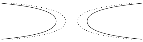
Figure 1. The boundary of the domain ${\widehat{\Omega}}$ over which the catenoid is a bigraph (dots) and the boundary of the corresponding exceptional domain $\Omega$ (solid). The domains have been rotated by $90^{\circ}$ so that the figure fits the page. Plotted with Maple.

7.3. Scherk’s simply periodic surface

This periodic surface depends on a parameter $\alpha\in(0,\frac{\pi}{2})$. Its Weierstrass data is usually written as:

$$\Sigma={\mathbb{C}}\cup\{\infty\}\setminus\{\pm e^{i\alpha},\pm e^{-i\alpha}\},\quad g_{{\mbox{\tiny Scherk}}}=z,\quad dh_{{\mbox{\tiny Scherk}}}=\frac{4\sin(2\alpha)\,z\,dz}{z^{4}-2\cos(2\alpha)\,z^{2}+1}.$$

This is actually the Weierstrass data of the surface in the quotient by its period which is the vertical vector $(0,0,2\pi)$. The immersion (11) is multi-valued on $\Sigma$ – the multi-valuation gives rise to the periodicity of the surface – and is well defined on a certain covering of $\Sigma$. This surface is a bigraph over the vertical plane $x_{1}=0$ and also over $x_{2}=0$. Using Point (2) of Proposition 5, we obtain the Weierstrass data of the horizontal Scherk surface (with horizontal period $(2\pi,0,0)$) which is a bigraph over the horizontal plane $x_{3}=0$:

$$g:=\frac{1+z}{1-z},\quad dh=\frac{2\sin(2\alpha)\,(1-z^{2})dz}{z^{4}-2\cos(2\alpha)\,z^{2}+1}.$$

Let $\sigma(z)=-\overline{z}$. Then $\sigma^{*}dh=-\overline{dh}$. Consequently, taking $p_{0}=0$ as base point, we have $X_{3}(z)=0$ on $i{\mathbb{R}}\cup\{\infty\}$. From the geometry of the Scherk surface, we know that this is precisely the zero set of $X_{3}$. To determine the sign of $X_{3}(z)$ in ${\rm Re}\,z>0$, we observe that $dh\simeq 2\sin(2\alpha)dz$ near $0$ so $X_{3}\simeq 2\sin(2\alpha)\,x$ near $0$. Hence $X_{3}>0$ in ${\rm Re}\,z>0$. Since $|g|>1$ in this domain, we use Point (1) of Proposition 5 and replace $g$ by $-1/g$. This gives

$$d\varphi=\frac{-2\sin(2\alpha)\,(z+1)^{2}dz}{z^{4}-2\cos(2\alpha)z^{2}+1}=-\frac{(z+1)^{2}}{2z}dh_{{\mbox{\tiny Scherk}}}.$$

Hence

$${\,\rm Res}_{e^{i\alpha}}d\varphi=-(1+\cos\alpha){\,\rm Res}_{e^{i\alpha}}dh_{{\mbox{\tiny Scherk}}}=i(1+\cos\alpha).$$

The residue at $e^{-i\alpha}$ is opposite by symmetry. Hence $\varphi$ is multi-valued on $\Sigma^{+}$, with multi-valuation equal to $2\pi(1+\cos\alpha)$. So $\Omega$ is a periodic domain with period

$$T_{\alpha}=2\pi(1+\cos\alpha).$$

Now the horizontal Scherk surface is a bigraph over a domain ${\widehat{\Omega}}$ which is bounded by a convex curve $\gamma$ together with its translates by multiples of $2\pi$. By Theorem 10, $\Omega$ is the domain bounded by $\gamma$ together with its translates by multiples of $T_{\alpha}$. This is a completely explicit geometric description of $\Omega$ (see Figure 2).

Figure 2. Top (dots): the boundary of the domain ${\widehat{\Omega}}$ over which the Scherk surface is a bigraph in the case $\alpha=\frac{\pi}{4}$. Bottom (solid): the boundary of the corresponding exceptional domain $\Omega$ (translated vertically so one can see something). Plotted with Maple.

It turns out that one can actually compute an equation of $\gamma$. Let us just give the main steps of the computation. The curve $\gamma$ is the image of the circle $i{\mathbb{R}}\cup\{\infty\}$ by $\varphi$. Then

$$\varphi(z)=-i\left[(1+\cos\alpha)\log\frac{z-e^{i\alpha}}{z-e^{-i\alpha}}+(1-\cos\alpha)\log\frac{z+e^{i\alpha}}{z+e^{-i\alpha}}\right].$$

Write $z=it$, $t\in{\mathbb{R}}$ and $\varphi(it)=(x(t),y(t))$. Then

$$x(t)=2\arctan\left(\frac{\sin(2\alpha)}{t^{2}+\cos(2\alpha)}\right),$$

$$y(t)=\cos\alpha\log\left(\frac{t^{2}+2\sin\alpha\,t+1}{t^{2}-2\sin\alpha\,t+1}\right).$$

Elimination of $t$ gives us an implicit equation of $\gamma$

(17) $$\cos^{2}\alpha\cosh(\frac{y}{\cos\alpha})=\sin^{2}\alpha+\cos(2\alpha-x).$$

(More precisely, $\gamma$ is the component of the solution set of (17) which goes through $0$.) In the particular case $\alpha=\frac{\pi}{4}$, Equation (17) simplifies to

$$\cosh(\sqrt{2}\,y)=1+2\sin x.$$

Remark 7.

Let $\Omega_{\alpha}$ be the exceptional domain corresponding to the Scherk surface of parameter $\alpha$. Using Equation (17), one can prove that:

• As $\alpha\to 0$, $\frac{1}{2\alpha}\Omega_{\alpha}$ converges to the domain $|z-1|>1$

• As $\alpha\to\frac{\pi}{2}$, $\frac{1}{\pi-2\alpha}\Omega_{\alpha}$ converges to the domain $|x+1+\frac{\pi}{2}|<\frac{\pi}{2}+\cosh y$.

The limit domains are, up to similitude, the examples of Sections 7.1 and 7.2. This corresponds to the well known fact that the horizontal Scherk surface, suitably scaled, converges to a vertical catenoid as $\alpha\to 0$ and a horizontal catenoid as $\alpha\to\frac{\pi}{2}$. As a consequence, if we consider as equivalent two domains which differ by a similitude, we can put all the examples of Sections 7.1, 7.2 and 7.3 in a continuous family $\Omega_{\alpha}$ for $\alpha\in[0,\frac{\pi}{2}]$: $\Omega_{0}$ is the example of Section 7.1 and $\Omega_{\frac{\pi}{2}}$ is the example of Section 7.2.

8. Classification results

Theorem 12.

Let $\Omega$ be an exceptional planar domain of finite connectivity (meaning that $\partial\Omega$ has a finite number of components). Then $\Omega$ is one of the following domains:

• a half-plane,

• the outside of a disk,

• the domain $|y|<\frac{\pi}{2}+\cosh x$, up to a similitude.

Assume that $\Omega$ is not a half-plane. By Theorem 1, $|\nabla u|<1$ in $\Omega$. Let $M$ be the minimal bigraph associated to $\Omega$ by Theorem 9. If $\partial\Omega$ is compact, then $M$ has two ends. By Theorem 2, $\lim_{z\to\infty}g(z)=0$. This implies that $M$ has finite total curvature. By a theorem of Schoen [23], an embedded minimal surface with finite total curvature and two ends is a catenoid. Since $g=0$ at the top end, $M$ is a vertical catenoid.

Else, let $k\geq 1$ be the number of proper arcs in $\partial\Omega$. Then $M$ has $k$ ends. By Theorem 6, $k\leq 2$ and the limit of the Gauss map at each end exists and is a complex number of norm 1. This implies that $M$ has finite total curvature. If $k=1$, then $M$ is vertical plane because the only embedded minimal surface with finite total curvature and one end is the plane. This is not possible because the vertical plane is not a bigraph. Hence $k=2$, and $M$ is a horizontal catenoid by the theorem of Schoen. $\Box$

Theorem 13.

Let $\Omega$ be a periodic exceptional domain. Assume that $\Omega$ has finite connectivity in the quotient. Then $\Omega$ is one of the following domains:

• a half-plane,

• the exceptional domain corresponding to a horizontal Scherk surface (namely, one of the domains described in Section 7.3, up to similitude).

Proof: Assume that $\Omega$ is not a half-plane. By Theorem 7, $|\nabla u|<1$ in $\Omega$. Let $M$ be the minimal bigraph associated to $\Omega$ by Theorem 9. Then $M$ is a periodic minimal surface with horizontal period $T$. By Theorem 7, $M^{+}/T$ is bounded by a finite number of Jordan curves in the plane $x_{3}=0$, and has at most two ends. Moreover, the Gauss map has a limit at each end, so $M/T$ has finite total curvature. By a theorem of Meeks-Rosenberg [18], the ends of $M/T$ are either of planar, helicoidal or Scherk type. In both the planar and helicoidal cases, $M^{+}/T$ would intersect the horizontal plane $x_{3}=0$ in a non-compact set. Hence $M/T$ has at most four Scherk-type ends. If $M/T$ has two Scherk-type ends then it is a plane, which is not possible. So it has four Scherk-type ends. By a theorem of Meeks-Wolf [19], $M$ is a Scherk surface. $\Box$

Remark 8.

The theorem of Meeks-Wolf is a difficult result. Moreover, Theorem 13 is equivalent to the Theorem of Meeks-Wolf: Indeed, using the Alexandrov moving plane method, one can prove that a periodic minimal surface with 4 Scherk-type ends must be a minimal bigraph over some plane. For this reason, I don’t think that there is an elementary proof of Theorem 13.

9. Immersed domains

In [14], the authors also propose to study Problem (1) on arbitrary flat Riemannian manifolds with boundary. They construct examples which have some analogy with immersed minimal surfaces called $k$-noids. This was another hint at the correspondence between exceptional domains and minimal surfaces. The correspondence, however, does not generalize to arbitrary flat surfaces. Let me propose a setup where the correspondence extends. This will allow us to recover the examples discussed in [14], and more. The following definitions are standard:

Definition 3.

1. A (smooth, 2-dimensional) immersed domain $\Omega$ is a smooth, complete, flat, 2-dimensional Riemannian manifold-with-boundary such that there exists a map $f:\Omega\to{\mathbb{C}}$ which is a local isometry, called the developing map of $\Omega$.

2. We say that $\Omega$ has embedded ends if the developing map is injective on each end of $\Omega$.

Note that by definition of a manifold-with-boundary, $\Omega$ includes its boundary. We will denote by $\mathring{\Omega}=\Omega\setminus\partial\Omega$ the set of interior points of $\Omega$. Here the word complete means that $\Omega$ is complete as a metric space. A flat Riemannian manifold always admits locally a developing map, but the developing map is in general not globally defined unless the manifold is simply connected. The definition of an immersed domain requires the developing map to be globally defined.

An immersed domain $\Omega$ (with non-empty boundary) is called exceptional if Problem (1) has a solution $u$ on $\Omega$ (where $\Delta u$ and $|\nabla u|$ are computed for the metric of $\Omega$). Theorem 1 generalizes to:

Theorem 14.

Let $\Omega$ be a non-trivial exceptional immersed domain with finite connectivity and embedded ends. Then $|\nabla u|<1$ in $\mathring{\Omega}$.

Proof: Theorem 1 is proved by showing that $|\nabla u|$ is bounded in each unbounded component of $\Omega\setminus D(0,R)$. Since we assume that our immersed domain has embedded ends, the proof carries over. $\Box$

Next we recall the definition of strong symmetry from [5], Definition 1. Let $X:M\to{\mathbb{R}}^{3}$ be an isometric immersion of a connected orientable surface $M$, and $\Pi$ be a plane in ${\mathbb{R}}^{3}$ which we normalize as the horizontal plane $x_{3}=0$. Denote by $S$ the symmetry with respect to the plane $x_{3}=0$, and

$$M^{+}=M\cap\{X_{3}>0\},\quad M^{-}=M\cap\{X_{3}<0\},\quad M^{0}=M\cap\{X_{3}=0\}.$$

Definition 4.

$M$ is strongly symmetric with respect to $\Pi$ if:

1. There exists an isometric involution $s:M\to M$ such that $X\circ s=S\circ X$,

2. The set of fixed points of $s$ is $M^{0}$,

3. The third coordinate $N_{3}$ of the Gauss map of $M$ takes positive (resp. negative) values on $M^{+}$ (resp. $M^{-}$).

With these definitions, Theorem 11 generalizes to:

Theorem 15.

There is a one-to-one correspondence between the following two classes of objets:

• immersed domains $\Omega$ which have finite connectivity, embedded ends and are homeomorphic to a planar domain,

• complete, immersed minimal surfaces $M$ which are strongly symmetric, have finite total curvature, embedded ends, and such that $M^{+}$ is homeomorphic to a planar domain.

There are plenty of such minimal surfaces. The basic example is the Jorge-Meeks $k$-noid, which has $k\geq 3$ horizontal catenoidal ends. Genus zero examples with $k\geq 3$ horizontal catenoidal ends are classified by C. Cosin and A. Ros in [5], they form a $2k-2$ parameters family which includes the Jorge-Meeks $k$-noid as the most symmetric member. The corresponding exceptional domains are the domains constructed in Section 4 of [14]. Genus one examples with $k\geq 3$ horizontal catenoidal ends are constructed by L. Mazet in [17]. Pictures of higher genus examples can be seen on the minimal surface archive of M. Weber [27].

Proof: Assume that we are given an exceptional immersed domain $\Omega$ with developing map $f$, satisfying all the hypothesis of Theorem 15. We define the holomorphic differential $dh$ by

$$dh=2d^{(1,0)}u=2u_{z}dz$$

where $z$ is a local conformal coordinate on $\Omega$. The holomorphic function $g$ is defined by

$$g=\frac{dh}{df}=\frac{2u_{z}}{f^{\prime}}.$$

Since $f$ is a local isometry, the metric of $\Omega$ in the local coordinate $z$ is $|f^{\prime}(z)dz|$. Hence

$$|\nabla u|=\frac{|2u_{z}|}{|f^{\prime}|}=|g|.$$

Let $M^{+}$ be the minimal surface parametrized on $\Omega$ by the Weierstrass Representation formula (11). To see that the immersion $X$ is well defined, consider the differential

$$d\psi=dX_{1}+i\,dX_{2}=\frac{1}{2}(\overline{g^{-1}dh}-gdh).$$

Then on the boundary of $\Omega$ we have

$$d\psi=\overline{g^{-1}dh}=\overline{df}.$$

Since the developing map is well defined in $\Omega$, $df$ is an exact differential. Since $\Omega$ is homeomorphic to a planar domain, $H_{1}(\Omega,{\mathbb{Z}})$ is generated by the closed curves in $\partial\Omega$. Hence $d\psi$ is an exact differential on $\Omega$ and $X$ is well defined. Since $X_{3}=0$ and $|g|=1$ on $\partial\Omega$, we may extend $M^{+}$ by symmetry with respect to the plane $x_{3}=0$ into a strongly symmetric immersed minimal surface $M$. The metric induced on $\Omega$ by the conformal immersion $X$ is

(18) $$ds=\frac{1}{2}(|g^{-1}dh|+|gdh|)=|df|\frac{1+|g|^{2}}{2}.$$

Since $|g|<1$ in $\Omega$, this implies that $M$ is complete. Let $E$ be an end of $\Omega$. There are two cases:

• If $f(E)$ is the complement of a bounded domain in ${\mathbb{C}}$, then $E$ is conformally a punctured disk and $df$ has a double pole at the puncture. Moreover, by Theorem 2, $|\nabla u|\to 0$ so $g$ has a zero at the puncture. This implies that $g^{-1}dh$, $gdh$ and $dh$ have at most double poles at the puncture. Since this characterizes embedded ends of finite total curvature, we conclude that the corresponding end of $M$ is embedded.

• If the boundary of $f(E)$ is not bounded: then by passing to a sub-end, we may assume that $f(E)$ is a concave domain bounded by $\alpha_{1}\cdot\alpha_{2}\cdot\alpha_{3}$, where $\alpha_{1}$ and $\alpha_{3}$ are proper arcs: $[0,\infty)\to{\mathbb{C}}$ and $\alpha_{2}$ is a straight segment connecting the endpoints of $\alpha_{1}$ and $\alpha_{3}$. The proof of Point (4) of Theorem 9 says that $\psi$ is injective on $E$, so $X(E)$ is a graph and the corresponding end of $M$ is embedded. (Indeed, if $z,z^{\prime}$ are two points in $f(E)$, the segment $[z,z^{\prime}]$ can only cross the boundary components $\alpha_{1}$ and $\alpha_{3}$.)

Finally, the fact that $g$ has a limit at each end implies that $M$ has finite total curvature.

Conversely, assume that we are given a minimal surface $M$ satisfying all the hypothesis of Theorem 15. Let $(\Sigma,g,dh)$ be the Weierstrass data of $M$. Since $M$ is strongly symmetric, the Riemann surface $\Sigma$ admits a antiholomorphic involution $s$ such that $X\circ s=S\circ X$. Moreover, the fixed set of $s$ divides $\Sigma$ into two components $\Sigma^{+}$ and $\Sigma^{-}$ such that $|g|<1$ in $\Sigma^{+}$ and $|g|>1$ in $\Sigma^{-}$. (Observe that since $M$ has finite total curvature, it is properly immersed, so the strong halfspace theorem of Hoffman Meeks (Theorem 2 in [15]) implies that $M^{+}$ is connected.) Consider the differential $df=g^{-1}dh$ in $\Sigma^{+}$. Since $g$ and $dh$ have the same zeros with same multiplicity, $df$ is holomorphic with no zeros in $\Sigma^{+}$. On the boundary of $\Sigma^{+}$, we have $df=\overline{d\psi}=dX_{1}-i\,dX_{2}$. Since $X$ is well defined and $\Sigma^{+}$ is homeomorphic to a planar domain, this implies that $df$ is exact. By integration, we obtain a well defined holomorphic function $f:\Sigma^{+}\to{\mathbb{C}}$ with non-zero derivative. We define $\Omega$ as $\Sigma^{+}$ with the conformal metric $|df|$ and $f$ as developing map. Formula (18) shows that the metric $|df|$ is equivalent to the metric $ds$ induced by the immersion $X$ on $\Sigma^{+}$. Hence $\Omega$ is complete, so is an immersed domain.

It remains to prove that $\Omega$ has embedded ends. Fix an end $E$ of $M$. Since $M$ is complete and has finite total curvature, Osserman’s theorem tells us that $E$ can be parametrized conformally on a punctured disk. Moreover, $g$ and $dh$ extend meromorphically at the puncture. Since $M$ is strongly symmetric, Lemma 4 in [5] tells us that the asymptotic normal at the end is either horizontal or vertical. Therefore, either $g=0$, $g=\infty$ or $|g|=1$ at the puncture corresponding to the end.

• If $g=0$ at the puncture, then the end can be parametrized on a punctured disk entirely included in $\Sigma^{+}$. Moreover, since the end is embedded, $g^{-1}dh$ has a double pole at the puncture. Therefore, $f$ has a simple pole, so is injective in a neighborhood of the end. This implies that the corresponding end of $\Omega$ is embedded (and asymptotic to a plane).

• If $g=\infty$ at the puncture, then the end can be parametrized on a punctured disk entirely contained in $\Sigma^{-}$, so we do not see it in $\Omega$.

• If $|g|=1$ at the puncture, then Point (b) of Lemma 4 in [5] says that the end is asymptotic to a horizontal catenoid. Therefore, $E^{+}=E\cap M^{+}$ is a graph over a concave domain $\widehat{E}$ in the plane, which we may take to be bounded by $\alpha_{1}\cdot\alpha_{2}\cdot\alpha_{3}$, where $\alpha_{1}$ and $\alpha_{3}$ are convex curves included in $M^{0}$ and $\alpha_{2}$ is a straight segment. The proof of Point (3) of Theorem 10 tells us that $f$ is injective in $E^{+}$. $\Box$

Martin Traizet
Laboratoire de Mathématiques et Physique Théorique
Université François Rabelais
37200 Tours, France.
email address: martin.traizet@lmpt.univ-tours.fr

References

- [1] S. Axler, P. Bourdon, W. Ramey: Harmonic Function Theory (Second Edition). Springer Verlag (2001).
- [2] G. R. Baker, P. G. Saffman, J. S. Sheffield: Structure of a linear array of hollow vortices of finite cross-section. J. Fluid Mech. 74, part 3 (1976), 469–476.
- [3] C. Bénéteau, D. Khavinson: The isoperimetric inequality via approximation theory and free boundary problems. Comp. Methods Function Theory 6, No 2 (2006), 253–274.
- [4] J.B. Conway: Functions of One Complex Variable (Second Edition). Graduate Texts in Mathematics 11. Springer Verlag (1986).
- [5] C. Cosin, A. Ros: A Plateau Problem at infinity for properly immersed minimal surfaces with finite total curvature. Indiana Univ. Math. J. 50, No. 2 (2001), 847–879.
- [6] D. Crowdy, C. Green: Analytical solutions for von Karman streets of hollow vortices. Physics of Fluids 23, 126602 (2011).
- [7] B. Daniel, L. Hauswirth. Half-space theorem, embedded minimal annuli and minimal graphs in the Heisenberg group. Proc. London Math. Soc. (3) 98 (2009), 445–470.
- [8] P. Duren: Univalent Functions. Grundlehren der mathematishen Wissenschaften 259. Springer Verlag (1983).
- [9] H. M. Farkas, I. Kra: Riemann Surfaces. Graduate texts in mathematics 72. Springer-Verlag (1980)
- [10] W.H.J. Fuchs: A Phragmen Lindelöf Theorem conjectured by D.J. Newman. Trans. Amer. Math. Soc. 267, No. 1 (1981), 285–293.
- [11] D. Gilbard, N.S. Trudinger: Elliptic Partial Differential Equations of Second order (Second Edition). Grundlehren der mathematischen Wissenschaften 224. Springer Verlag (1983)
- [12] A. Gray: Modern differential geometry of curves and surfaces. Studies in Advanced Mathematics (1993).
- [13] R. Greene, S. Krantz: Function theory of one complex variable (Third Edition). Graduate Studies in Mathematics, volume 40. Amer. Math. Soc. (2006).
- [14] F. Hélein, L. Hauswirth, F. Pacard: A note on some overdetermined elliptic problem. Pacific J. Math. 250 (2011), 319–334.
- [15] D. Hoffman, W.H. Meeks III: The strong halfspace theorem for minimal surfaces. Invent. Math. 101 (1990), 373–377.
- [16] D. Khavinson, E. Lundberg, R. Teodorescu: An overdetermined problem in potential theory. arXiv:1205.5165v2 (2012).
- [17] L. Mazet: The Plateau problem at infinity for horizontal ends and genus 1. Indiana Univ. Math. J. 55 (2006), 15–64.
- [18] W.H. Meeks III, H. Rosenberg: The geometry of periodic minimal surfaces. Comment. Math. Helvetici 68 (1993) 538–578.
- [19] W. H. Meeks III, M. Wolf: Minimal surfaces with the area growth of two planes; the case of infinite symmetry. Journal of the A.M.S. 20, No. 2 (2007), 441–465.
- [20] S. Montiel, A. Ros: Curves and Surfaces. Graduate Studies in Mathematics, volume 69. Amer. Math. Soc. (2005).
- [21] J. Pérez, A. Ros: Properly embedded minimal surfaces with finite total curvature. The Global Theory of Minimal Surfaces in Flat Spaces, Lecture Notes in Math. 1775 (2002), 15–66.
- [22] A. Ros, P. Sicbaldi: Geometry and topology of some overdetermined elliptic problems. arXiv:1202.5167 (2012).
- [23] R. Schoen: Uniqueness, symmetry and embeddedness of minimal surfaces. J. Diff. Geom. 18 (1983), 791-809.
- [24] R. Schoen: Estimates for Stable Minimal Surfaces in Three Dimensional Manifolds. Seminar on Minimal Submanifolds, Ann. of Math. Studies 103 (1983), 111–126.
- [25] J. Serrin: A symmetry problem in potential theory. Archive for Rational Mechanics and Analysis 43, no 4 (1971), 304–318.
- [26] F. Schlenk, P. Sicbaldi: Bifurcating extremal domains for the first eigenvalue of the Laplacian. Adv. Math. 229 (2012), 602-632.
-
[27]
Matthias Weber: Minimal Surface Archive.
http://www.indiana.edu/~minimal/archive.