Hierarchical Liouville-space approach to nonequilibrium dynamical properties of quantum impurity systems

Abstract

We propose a hierarchical dynamics approach for evaluation of nonequilibrium dynamic response properties of quantum impurity systems. It is based on a hierarchical equations of motion formalism, in conjunction with a linear response theory established in the hierarchical Liouville space. This provides an accurate and universal tool for characterization of a variety of response and correlation functions of local impurities, as well as transport related response properties. The practicality of our proposed approach is demonstrated via the evaluation of various dynamical properties of a single-impurity Anderson model. These include the impurity spectral density, local charge fluctuation, local magnetic susceptibility, and current-voltage admittance, in both equilibrium and nonequilibrium situations. The numerical results are considered to be quantitatively accurate, as long as they converge quantitatively with respect to the truncation of the hierarchy.

I Introduction

Recent advances in fabrication, manipulation and measurement of artificial quantum impurity systems such as quantum dots have led to a resurgence of interest of nanostructures in both experiment and theory. A favorable feature of these nanostructures is the outstanding tunability of device parameters. Understanding the dynamical properties of quantum impurity systems is of fundamental importance for the development of solid-state quantum information processingElz04431 ; Kop06766 ; Han081043 and single-electron devices. Gab06499 ; Fev071169 Moveover, quantum impurity models serve as essential theoretical tools, covering a broad range of important physical systems. For instance, the Hubbard lattice model can be mapped onto the Anderson impurity model via a self-consistent dynamical mean field theory.Met89324 ; Geo926479 ; Geo9613 Besides the strong electron-electron (e-e) interactions, local impurities are also subject to interactions with itinerant electrons in surrounding bulk materials, which serve as the electron reservoir as well as thermal bath. The interplay between the local e-e interactions and nonlocal transfer coupling gives rise to a variety of intriguing phenomena of prominent many-body nature, such as Kondo effect,Cro98540 ; Gol98156 ; Bul08395 Mott metal-insulator transition,Geo921240 ; Ima981039 ; Bul01045103 and high-temperature superconductivity.Eme872794 ; Yan031 ; Mai05237001

Characterizing the system responses to external perturbation of experimental relevance is of fundamental significance in understanding the intrinsic properties of quantum impurity systems and their potential applications. For instance, the magnetic susceptibility of an impurity system reflects the redistribution of electron spin under an applied magnetic field, and its investigation may have important implications for fields such as spintronics.

For the accurate characterization of dynamical properties of the impurity such as the impurity spectral function and dynamical charge/magnetic susceptibility, a variety of nonperturbative numerical approaches have been developed, such as numerical renormalization group method,Wil75773 ; Hof001508 ; Bul08395 density matrix renormalization group approach,Whi922863 ; Jec02045114 ; Nis04613 and quantum Monte Carlo method. Hir862521 ; Sil902380 ; Gub916011 ; Gul11349 While most of work has focused on equilibrium properties, the accurate characterization of nonequilibrium dynamical properties has remained very challenging.

In many experimental setups,Gol98156 ; Cro98540 artificial quantum impurity systems attached to electron reservoirs are subject to applied bias voltages. This stimulates the experimental and theoretical exploration of nonequilibrium processes in quantum impurity systems. A variety of interesting physical phenomena have been observed, which originate from the interplay between strong electron correlation and nonequilibrium dissipation.Doy06245326 ; Meh08086804 ; Bou08140601 ; Chu09216803

In the past few years, a number of nonperturbative theoretical approaches have been devised to treat systems away from equilibrium. These include the time-dependent numerical renormalization group method,Cos973003 ; And05196801 ; And08066804 time-dependent density matrix renormalization group method,Whi04076401 nonequilibrium functional renormalization group,Jak07150603 ; Gez07045324 quantum Monte Carlo method,Han99236808 ; Wer09035320 ; Sch09153302 iterative real-time path integral approach,Wei08195316 ; Seg10205323 and nonequilibrium Bethe ansatz.Kon01236801 ; Meh06216802 ; Cha11195314 Despite the progress made, quantitative accuracy is not guaranteed for the resulted nonequilibrium properties, because of the various simplifications and approximations involved in these approaches. Therefore, an accurate and universal approach which is capable of addressing nonequilibrium situations is highly desirable.

In this work we propose a hierarchical dynamics approach for the characterization of nonequilibrium response of local impurities to external fields. A general hierarchical equations of motion (HEOM) approach has been developed, Jin08234703 ; Zhe09164708 ; Zhe121129 which describes the reduced dynamics of open dissipative systems under arbitrary time-dependent external fields. The HEOM theory resolves the combined effects of e-e interactions, impurity-reservoir dissipation, and non-Markovian memory in a nonperturbative manner. In the framework of HEOM, the nonequilibrium dynamics are treated by following the same numerical procedures as in equilibrium situations. The HEOM theory is in principle exact for an arbitrary equilibrium or nonequilibrium system, provided that the full hierarchy inclusive of infinite levels are taken into account.Jin08234703 In practice, the hierarchy needs to be truncated at a finite level for numerical tractability. The convergence of calculation results with respect to the truncation level should be carefully examined. Once the convergence is achieved, the numerical outcome is considered to reach quantitative accuracy for systems in both equilibrium and nonequilibrium situations.

It has been demonstrated that the HEOM approach leads to an accurate and universal characterization of strong electron correlation effects in quantum impurity systems, and treats the equilibrium and nonequilibrium scenarios in a unified manner. For the equilibrium properties of Anderson model systems, the HEOM approach achieves the same level of accuracy as the latest state-of-the-art NRG method.Li12266403 In particular, the universal Kondo scaling of zero-bias conductance and the logarithmic Kondo spectral tail have been reproduced quantitatively. For systems out of equilibrium, numerical calculations achieving quantitative accuracy remain very scarce. One of the rare cases where numerically exact solution is available is the dynamic current response of a noninteracting quantum dot to a step-pulse voltage. Ste04195318 ; Mac06085324 This has been precisely reproduced by the HEOM approach. Zhe08184112 However, there are very few calculations at the level of quantitative accuracy for systems involving strong e-e interactions, since most of the existing methods involve intrinsic approximations. Based on the HEOM formalism, quantitative accuracy should be achieved once the numerical convergence with respect to the truncation level of hierarchy is reached.

There are two schemes to evaluate the response properties of quantum impurity systems in the framework of HEOM: (i) Calculate relevant system correlation/response functions based on a linear response theory constructed in the HEOM Liouville space;Li12266403 and (ii) solve the EOM for a hierarchical set of density operators to obtain the transient reduced dynamics of system in response to time-dependent external perturbation, followed by a finite difference analysis. These two schemes are completely equivalent in the linear response regime, as have been verified numerically. In previous studies, we had employed the above second scheme to evaluate the dynamic admittance (frequency-dependent electric current in response to external voltage applied to coupling electron reservoirs) of quantum dot systems, which had led to the identification of several interesting phenomena, including dynamic Coulomb blockadeZhe08093016 and dynamic Kondo transition,Zhe09164708 and photon-phonon-assisted transport.Jia12245427

In this work, we will elaborate the above first scheme of HEOM approach. The external perturbation may associate with an arbitrary operator in the impurities subspace, or originates from a homogeneous shift of electrostatic potential (and hence the chemical potential) of electron reservoir. The detailed numerical procedures will be exemplified through the evaluation of a variety of response properties of a single-impurity Anderson model, including the impurity spectral density function, local charge fluctuation spectrum, local magnetic susceptibility, and dynamic admittance.

The remainder of paper is organized as follows. We will first give a brief introduction on the HEOM method in Sec. II. In Sec. III we will elaborate the establishment of a linear response theory in the HEOM Liouville space. Calculation on system correlation/response functions which are directly relevant to the response properties of primary interest will be discussed in detail. We will then provide numerical demonstrations for the evaluation of various dynamical properties in Sec. IV. Finally, the concluding remarks will be given in Sec. V.

II A real-time dynamics theory for nonequilibrium impurity systems

II.1 Prelude

Consider a quantum impurity system in contact with two electron reservoirs, denoted as the $\alpha=$ L and R reservoirs, under the bias voltage $V=\mu_{\rm L}-\mu_{\rm R}$. The total Hamiltonian of the composite system assumes the form of

$$H_{{\rm total}} =H_{\text{\scriptsize sys}}+\sum_{\alpha k}(\epsilon_{\alpha k}+\mu_{\alpha})\,\hat{d}^{\dagger}_{\alpha k}\hat{d}_{\alpha k}$$

$$\quad+\sum_{\alpha\mu k}\left(t_{\alpha k\mu}\hat{d}^{\dagger}_{\alpha k}\hat{a}_{\mu}+{\rm H.c.}\right).$$ (1)

The impurity system Hamiltonian $H_{\text{\scriptsize sys}}$ is rather general, including many-particle interactions and external field coupling. Its second quantization form is given in terms of electron creation and annihilation operators, $\hat{a}^{\dagger}_{\mu}\equiv\hat{a}^{+}_{\mu}$ and $\hat{a}_{\mu}\equiv\hat{a}^{-}_{\mu}$, which are associated with the system spin-state $\mu$. The reservoirs are modeled by a noninteracting Hamiltonian; see the second term on the right-hand side (rhs) of Eq. (II.1), where $\hat{d}^{\dagger}_{\alpha k}$ ($\hat{d}_{\alpha k}$) and $\epsilon_{\alpha k}$ are the creation (annihilation) operator and energy of single-electron state $|k\rangle$ electron of $\alpha$-reservoir, respectively. While the equilibrium chemical potential of total system is set to be $\mu^{\rm eq}_{\alpha}=0$, the reservoir states are subject to a homogeneous shift, $\mu_{\alpha}$, under applied voltages. The last term on the rhs of Eq. (II.1) is in a standard transfer coupling form, which is responsible for the dissipative interactions between the system and itinerary electrons of reservoirs. It can be recast as $H^{\prime}=\sum_{\alpha\mu}(\hat{f}^{+}_{\alpha\mu}\hat{a}^{-}_{\mu}+\hat{a}^{+}_{\mu}\hat{f}^{-}_{\alpha\mu})$, where $\hat{f}^{+}_{\alpha\mu}\equiv\sum_{k}t_{\alpha k\mu}\hat{d}^{\dagger}_{\alpha k}=\big{(}\hat{f}^{-}_{\alpha\mu}\big{)}^{\dagger}$. Throughout this paper we adopt the atomic unit $e=\hbar=1$ and denote $\beta=1/(k_{B}T)$, with $k_{B}$ being the Boltzmann constant and $T$ the temperature of electron reservoirs. Introduce also the sign variables, $\sigma=+/-$ and $\bar{\sigma}\equiv-\sigma$ the opposite sign of $\sigma$.

The $\alpha$-reservoir is characterized by the spectral density $J_{\alpha\mu\nu}(\omega)\equiv\pi\sum_{k}t^{\ast}_{\alpha k\mu}t_{\alpha k\nu}\delta(\omega-\epsilon_{\alpha k})$. It influences the dynamics of reduced system through the reservoir correlation functions $\tilde{C}^{\sigma;{\rm st}}_{\alpha\mu\nu}(t-\tau)\equiv\langle\hat{f}^{\sigma}_{\alpha\mu}(t)\hat{f}^{\bar{\sigma}}_{\alpha\nu}(\tau)\rangle_{\alpha}$, Here, $\langle(\cdot)\rangle_{\alpha}\equiv{\rm tr}_{\alpha}\big{[}(\cdot)\,e^{-\beta H_{\alpha}}\big{]}/{\rm tr}_{\alpha}(e^{-\beta H_{\alpha}})$ and $\hat{f}^{\sigma}_{\alpha\mu}(t)\equiv e^{iH_{\alpha}t}\hat{f}^{\sigma}_{\alpha\mu}e^{-iH_{\alpha}t}$, with $H_{\alpha}$ being the Hamiltonian of $\alpha$-reservoir. The superscript “st” highlights the stationary feature of the nonequilibrium correlation function, under a constant $\mu_{\alpha}$. It is related to the reservoir spectral density, $J_{\alpha\mu\nu}(\omega)\equiv J^{-}_{\alpha\mu\nu}(\omega)\equiv J^{+}_{\alpha\nu\mu}(\omega)$, via the fluctuation-dissipation theorem: Jin08234703

$$\tilde{C}^{\sigma;{\rm st}}_{\alpha\mu\nu}(t)=\int_{-\infty}^{\infty}\!d\omega\frac{e^{\sigma i\omega t}J^{\sigma}_{\alpha\mu\nu}(\omega-\mu_{\alpha})}{1+e^{\sigma\beta(\omega-\mu_{\alpha})}}.$$ (2)

Physically, $\tilde{C}^{\sigma;{\rm st}}_{\alpha\mu\nu}(t)$, with $\sigma=+$ or $-$, describes the processes of electron tunneling from the $\alpha$-reservoir into the specified system coherent state or the reverse events, respectively.

We will be interested in nonequilibrium dynamic responses to a time-dependent external field acting on either the local system or the reservoirs. For the latter case, we include a time-dependent shift in chemical potential $\delta\Delta_{\alpha}(t)$, on top of the constant $\mu_{\alpha}$, to the $\alpha$-reservoir. Its effect can be described by rigid homogeneous shifts for the reservoir conduction bands, resulting in the nonstationary reservoir correlation functions of

$$C^{\sigma}_{\alpha\mu\nu}(t,\tau)=\exp\left[\sigma i\!\int_{\tau}^{t}\!{\rm d}t^{\prime}\,\delta\Delta_{\alpha}(t^{\prime})\right]\tilde{C}^{\sigma;{\rm st}}_{\alpha\mu\nu}(t-\tau).$$ (3)

This is the generalization of $\tilde{C}^{\sigma;{\rm st}}_{\alpha\mu\nu}(t)=e^{\sigma i\mu_{\alpha}t}\tilde{C}^{\sigma;{\rm eq}}_{\alpha\mu\nu}(t)$, as inferred from Eq. (2), with the equilibrium counterpart being of $\mu^{\rm eq}_{\alpha}=0$. In the following, we focus on the situation of diagonal reservoir correlation, i.e., $J^{\sigma}_{\alpha\mu\nu}(\omega)=J^{\sigma}_{\alpha\mu\mu}(\omega)\,\delta_{\mu\nu}$, and $\tilde{C}^{\sigma;{\rm st}}_{\alpha\mu\nu}(t)=\tilde{C}^{\sigma;{\rm st}}_{\alpha\mu\mu}(t)\,\delta_{\mu\nu}$. In constructing closed HEOM,Jin08234703 we should expand $\tilde{C}^{\sigma;{\rm st}}_{\alpha\mu\mu}(t)$ in a finite exponential series,

$$\tilde{C}^{\sigma;{\rm st}}_{\alpha\mu\mu}(t)\simeq\sum_{m=1}^{M}\eta^{\sigma}_{\alpha\mu m}e^{-\gamma^{\sigma}_{\alpha\mu m}t}.$$ (4)

Involved are a total number of $M=N^{\prime}+N$ poles from the reservoir spectral density and the Fermi function in the contour integration evaluation of Eq. (2). Various sum-over-poles schemes have been developed, including the Matsubara spectrum decomposition scheme,Jin08234703 a hybrid spectrum decomposition and frequency dispersion scheme,Zhe09164708 the partial fractional decomposition scheme,Cro09073102 and the Padé spectrum decomposition (PSD) scheme,Hu10101106 ; Hu11244106 with the primary focus on the Fermi function. To our knowledge, the PSD scheme has the best performance until now. We will come back to this issue later; see the remark-(6) in Sec. II.2. In the present work we use the $[N\!-\!1/N]$ PSD scheme.Hu10101106 ; Hu11244106 It leads to a minimum $M=N^{\prime}+N$ in the exponential expansion of Eq. (4) and thus an optimal HEOM construction.Jin08234703

The exponential expansion form of the reservoir correlation function in Eq. (4) dictates the explicit expressions for the HEOM formalism.Jin08234703 For bookkeeping we introduce the abbreviated index $j=\{\sigma\alpha\mu m\}$ for $\gamma_{j}\equiv\gamma^{\sigma}_{\alpha\mu m}$ and so on, or $j=\{\sigma\mu\}$ for $\hat{a}_{j}\equiv\hat{a}^{\sigma}_{\mu}$. Denote also $\bar{j}=\{\bar{\sigma}\alpha\mu m\}$ or $\{\bar{\sigma}\mu\}$ whenever appropriate, with $\bar{\sigma}$ being the opposite sign of $\sigma=+$ or $-$. The dynamical variables in HEOM are a set of auxiliary density operators (ADOs), $\{\rho^{(n)}_{j_{1}\cdots j_{n}}(t);n=0,1,\cdots,L\}$, with $L$ being the terminal or truncated tier of hierarchy. The zeroth-tier ADO is set to be the reduced system density matrix, $\rho^{(0)}(t)\equiv\rho(t)\equiv{\rm tr}_{\text{\scriptsize bath}}\,[\rho_{{\rm total}}(t)]$, i.e., the trace of the total system and bath composite density matrix over reservoir bath degrees of freedom.

II.2 Hierarchical equations of motion formalism

The HEOM formalism has been constructed from the Feynman–Vernon influence functional path integral theory, together with the Grassmann algebra.Jin08234703 The initial system-bath decoupling used for expressing explicitly the influence functional is set at the infinite past. It does not introduce any approximation for the characterization of any realistic physical process starting from a stationary state, which is defined via the HEOM that includes the coherence between the system and bath. The detailed construction of HEOM is referred to Ref. Jin08234703, . Here we just briefly introduce the HEOM formalism and discuss some of its key features.

The final HEOM formalism readsJin08234703

$$\dot{\rho}^{(n)}_{j_{1}\cdots j_{n}}= -\big{[}i{\cal L}(t)+\gamma^{(n)}_{j_{1}\cdots j_{n}}\!(t)\big{]}\rho^{(n)}_{j_{1}\cdots j_{n}}-i\sideset{}{{}^{\prime}}{\sum}_{j}{\cal A}_{\bar{j}}\,\rho^{(n+1)}_{j_{1}\cdots j_{n}j}$$

$$-i\sum_{r=1}^{n}(-)^{n-r}\,{\cal C}_{j_{r}}\,\rho^{(n-1)}_{j_{1}\cdots j_{r-1}j_{r+1}\cdots j_{n}}\,.$$ (5)

The boundary conditions are $\gamma^{(0)}=\rho^{(-1)}=0$, together with a truncation by setting all $\rho^{(n>L)}=0$. The initial conditions to Eq. (II.2) will be specified in conjunction with the evaluation of various response and correlation functions in Sec. III.

The time-dependent damping parameter $\gamma^{(n)}_{j_{1}\cdots j_{n}}\!(t)$ in Eq. (II.2) collects the exponents of nonstationary reservoir correlation function [cf. Eqs. (3) and (4)]:

$$\gamma^{(n)}_{j_{1}\cdots j_{n}}\!(t)=\sum_{r=1}^{n}\big{[}\gamma_{j_{r}}-\sigma i\delta\Delta_{\alpha}(t)\big{]}_{\sigma,\alpha\in j_{r}}.$$ (6)

This expression has been used directly in the HEOM evaluation of transient current dynamical properties under the influence of arbitrary time-dependent chemical potentials applied to electrode leads.Zhe08184112 ; Zhe08093016 ; Zhe09124508 ; Zhe09164708 Note that $\gamma_{j}\equiv\gamma^{\sigma}_{\alpha\mu m}=\gamma^{\sigma;{\rm eq}}_{\alpha\mu m}-\sigma i\mu_{\alpha}$. In Sec. III.3, we will treat $\delta\Delta_{\alpha}(t)$ as perturbation and derive the corresponding linear response theory formulations for various transport current related properties under nonequilibrium ($\mu_{\alpha}\neq 0$) conditions.

To evaluate nonequilibrium correlation functions of local system via linear response theory (cf. Sec. III.2), the time-dependent reduced system Liouvillian in Eq. (II.2) is assumed formally the form of

$$\mathcal{L}(t)=\mathcal{L}_{s}+\delta\mathcal{L}(t).$$ (7)

Here, $\mathcal{L}_{s}\,\cdot\,\equiv[H_{\text{\scriptsize sys}},\,\cdot\,]$ remains the commutator form involving two $H_{\text{\scriptsize sys}}$-actions onto the bra and ket sides individually. However, the time-dependent perturbation $\delta{\cal L}(t)$ may act only on one side, in line with the HEOM expressions for local system correlation functions.Mo05084115 ; Zhu115678 ; Xu11497 ; Xu13024106 ; Li12266403

Other features of HEOM and remarks, covering both the theoretical formulation and numerical implementation aspects, are summarized as follows.

(1) The Fermi-Grassmannian properties: (i) All $j$-indexes in a nonzero $n^{\rm th}$-tier ADO, $\rho^{(n)}_{j_{1}\cdots j_{n}}$, must be distinct. Swap in any two of them leads to a minus sign, such as $\rho^{(2)}_{j_{2}j_{1}}=-\rho^{(2)}_{j_{1}j_{2}}$. In line with this property, the sum of the tier-up dependence in Eq. (II.2) runs only over $j\not\in\{j_{1},\cdots,j_{n}\}$; (ii) Involved in Eq. (II.2) are also ${\cal A}_{\bar{j}}\equiv{\cal A}^{\bar{\sigma}}_{\mu}$ and ${\cal C}_{j}\equiv{\cal C}^{\sigma}_{\alpha\mu m}$. They are Grassmann superoperators, defined via their actions on an arbitrary operator of fermionic or bosonic (bi-fermion) nature, $\hat{O}^{\text{\tiny F}}$ or $\hat{O}^{\text{\tiny B}}$, by

$$\begin{split}{\cal A}_{\bar{j}}\hat{O}^{\text{\tiny F/B}}&\equiv\hat{a}_{\bar{j}}\hat{O}^{\text{\tiny F/B}}\mp\hat{O}^{\text{\tiny F/B}}\hat{a}_{\bar{j}}\,,\\ {\cal C}_{j}\hat{O}^{\text{\tiny F/B}}&\equiv\eta_{j}\hat{a}_{j}\hat{O}^{\text{\tiny F/B}}\pm\eta_{\bar{j}}^{\ast}\hat{O}^{\text{\tiny F/B}}\hat{a}_{j}\,.\end{split}$$ (8)

In particular, even-tier ADOs are bosonic, while odd-tier ones are fermionic. The case of opposite parity would also appear in conjunction with applications; see comments following Eq. (19).

(2) Physical contents of ADOs: While the zero-tier ADO is the reduced density matrix, i.e., $\rho^{(0)}(t)=\rho(t)$, the first-tier ADOs, $\rho^{(1)}_{j}\equiv\rho^{\sigma}_{\alpha\mu m}$, are related to the electric current through the interface between the system and $\alpha$-reservoir, $I_{\alpha}(t)$, as follows,

$$I_{\alpha}(t)=-2\,{\rm Im}\sum_{\mu m}{\rm Tr}\left[\hat{a}^{+}_{\mu}\rho^{-}_{\alpha\mu m}(t)\right].$$ (9)

Moreover, we have $\sum_{m}\rho^{\sigma}_{\alpha\mu m}(t)={\rm tr}_{\text{\scriptsize bath}}[\hat{f}^{\sigma}_{\alpha\mu}(t)\rho_{{\rm total}}(t)]$, and can further relate ${\rm tr}_{\text{\scriptsize bath}}[\hat{f}^{\sigma}_{\alpha\mu}(t)\hat{f}^{\sigma^{\prime}}_{\alpha^{\prime}\mu^{\prime}}(t)\rho_{{\rm total}}(t)]$ to the second-tier ADOs, and so on. Note that $\hat{f}^{+}_{\alpha\mu}(t)\equiv e^{iH_{\alpha}t}\big{(}\sum_{k}t_{\alpha k\mu}\hat{d}^{\dagger}_{\alpha k}\big{)}e^{-iH_{\alpha}t}=\big{[}\hat{f}^{-}_{\alpha\mu}(t)\big{]}^{\dagger}$ are defined in the bath-space only. Apparently, the Fermi-Grassmannian properties in remark-(1) above are rooted at the fermionic nature of individual $\{\hat{f}^{\sigma}_{\alpha\mu}\}$.

(3) Hermitian property: The ADOs satisfy the Hermitian relation of $\big{[}\rho^{(n)}_{j_{1}\cdots j_{n}}(t)\big{]}^{\dagger}=\rho^{(n)}_{{\bar{j}}_{n}\cdots{\bar{j}}_{1}}(t)$, whenever the perturbed $i\delta{\cal L}(t)$ action assumes Hermitian; see the comments following Eq. (7).

(4) Nonperturbative nature: The HEOM construction treats properly the combined effects of system-bath coupling strength, Coulomb interaction, and bath memory time scales, as inferred from the following observations. (i) For noninteracting electronic systems, the coupling hierarchy stops at second tier level ($L=2$) without approximation;Jin08234703 (ii) HEOM is of finite support, containing in general only a finite number of ADOs. Let $K$ be the number of all distinct $j$-indexes. Such a number draws the maximum tier level $L_{\text{max}}=K$, at which the HEOM formalism ultimately terminates. The total number of ADOs, up to the truncated tier level $L$, is $\sum^{L}_{n=0}\frac{K!}{n!(K-n)!}\leq 2^{K}$, as $L\leq L_{\text{max}}=K$; (iii) The hierarchy resolves collectively the memory contents, as decomposed in the exponential expansion of bath correlation functions of Eq. (4). It goes with the observation that an individual ADO, $\rho^{(n)}_{j_{1}\cdots j_{n}}$, is associated with the collective damping constant Re $\gamma^{(n)}_{j_{1}\cdots j_{n}}$ in Eq. (6). Meanwhile $\rho^{(n)}_{j_{1}\cdots j_{n}}$ has the leading $(2n)^{\rm th}$-order in the overall system-bath coupling strength. One may define proper non-Marvokianicity parameters to determine in advance the numerical importance of individual ADOs;Xu05041103 ; Shi09084105 ; Xu13024106 (iv) Convergency tests by far – For quantum impurity systems with nonzero e-e interactions, calculations often converge rapidly and uniformly with the increasing truncation level $L$. Quantitatively accurate results are usually achieved at a relatively low value of $L$.

(5) Nonequilibrium versus equilibrium: The HEOM formalism presented earlier provides a unified approach to equilibrium, nonequilibrium, time-dependent and time-independent situations. In general, the number $K$ of distinct ADO indexes amounts to $K=2N_{\alpha}N_{\mu}M$, as inferred from Eq. (4), with $N_{\mu}$ being the number spin-orbitals of system in direct contact to leads. The factor 2 accounts for the two choices of the sign variable $\sigma$, while $N_{\alpha}=2$ for the distinct $\alpha=$ L and R leads. Interestingly, in the equilibrium case, together with the $J_{\rm L}(\omega)\propto J_{\rm R}(\omega)$ condition, one can merger all leads into a single lead to have the reduced $K=2N_{\mu}M$. The resulting equilibrium HEOM formalism that contains no longer the $\alpha$-index can therefore be evaluated at the considerably reduced computational cost.

(6) Control of accuracy and efficiency: The bath correlation function in exponential expansion of Eq. (4) dictates the accuracy and efficiency of the HEOM approach. (i) The accuracy in the exponential expansion of Eq. (4) is found to be directly transferable to the accuracy of HEOM. In other words, HEOM is exact as long as the expansion is exact; (ii) The expansion of Eq. (4) is uniformly convergent, and becomes exact when $M$ goes to infinity, for any realistic bath spectral density with finite bandwidth at finite temperature ($T\neq 0$); (iii) The $[N\!-\!1/N]$ PSD scheme adopted in this work is considered to be the best among all possible sum-over-poles expansion of Fermi function.Hu10101106 ; Hu11244106 ; Bak96 In particular it is dramatically superior over the commonly used Matsubara expansion expression. The PSD scheme leads to the optimal HEOM, with a minimum $K$-space size, for either equilibrium or nonequilibrium case, as discussed in remark-(5) above.

(7) Computational cost: The CPU time and memory space required for HEOM calculations are rather insensitive to the Coulomb coupling strength and to the equilibrium versus nonequilibrium and time-dependent and time-independent types of evaluations. However, it grows exponentially as the temperature $T\rightarrow 0$, with respect to system-bath hybridization strength, due to the significant increase of both the converged $K$-space and $L$-space sizes.

To conclude, HEOM is an accurate and versatile tool, capable of universal characterizations of real-time dynamics in quantum impurity systems, in both equilibrium and nonequilibrium cases. These remarkable features have been demonstrated recently in several complex quantum impurity systems,Li12266403 with the focus mainly on equilibrium properties. The HEOM approach is also very efficient. Calculations often converge rapidly and uniformly with the increasing truncation level $L$. Quantitatively accurate results are usually achieved at a relatively low level of truncation.Li12266403 We will show in Sec. IV that these features will largely remain in the evaluations of nonequilibrium properties.

III Nonequilibrium response theory

III.1 Linearity of the hierarchical Liouville space

To highlight the linearity of HEOM, we arrange the involving ADOs in a column vector, denoted symbolically as

$${\bm{\rho}}(t)\equiv\big{\{}\rho(t),\,\rho^{(1)}_{j}\!(t),\,\rho^{(2)}_{j_{1}\!j_{2}}\!(t),\,\cdots\,\big{\}}.$$ (10)

Thus, Eq. (II.2) can be recast in a matrix-vector form (each element of the vector in Eq. (10) is a matrix) as follows,

$$\dot{\bm{\rho}}=-i\mbox{\boldmath${\cal L}$}(t)\bm{\rho},$$ (11)

with the time-dependent hierarchical-space Liouvillian, as inferred from Eqs. (II.2)–(7), being of

$$\mbox{\boldmath${\cal L}$}(t)=\mbox{\boldmath${\cal L}$}_{s}+\delta\mathcal{L}(t){\mbox{\boldmath${\cal I}$}}+\delta{\mbox{\boldmath${\cal V}$}}(t)\,.$$ (12)

It consists not just the time-independent $\mbox{\boldmath${\cal L}$}_{s}$ part, but also two time-dependent parts and each of them will be treated as perturbation at the linear response level soon. Specifically, $\delta\mathcal{L}(t){\mbox{\boldmath${\cal I}$}}$, with ${\cal I}$ denoting the unit operator in the hierarchical Liouville space, is attributed to a time-dependent external field acting on the reduced system, while $\delta{\mbox{\boldmath${\cal V}$}}(t)$ is diagonal and due to the time-dependent potentials $\delta\Delta_{\alpha}(t)$ applied to electrodes.

We may denote $\delta\Delta_{\alpha}(t)=x_{\alpha}\delta\Delta(t)$, with $0\leq x_{\rm L}\equiv 1+x_{\rm R}\leq 1$; thus $\delta\Delta(t)=\delta\Delta_{\rm L}(t)-\delta\Delta_{\rm R}(t)$. It specifies the additional time-dependent bias voltage, on top of the constant $V=\mu_{\rm L}-\mu_{\rm R}$, applied across the two reservoirs. As inferred from Eq. (6), we have then

$$\delta{\mbox{\boldmath${\cal V}$}}(t)=-{\mbox{\boldmath${\cal S}$}}\,\delta\Delta(t),$$ (13)

where ${\mbox{\boldmath${\cal S}$}}\equiv\text{diag}\big{\{}0,S^{(n)}_{j_{1}\cdots j_{n}};n=1,\cdots,L\big{\}}$, with

$$S^{(n)}_{j_{1}\cdots j_{n}}\equiv\sum_{r=1}^{n}\big{(}\sigma x_{\alpha}\big{)}_{\sigma,\alpha\,\in j_{r}}.$$ (14)

Note that $S^{(0)}=0$.

The additivity of Eq. (12) and the linearity of HEOM lead readily to the interaction picture of the HEOM dynamics in response to the time-dependent external disturbance $\delta\mbox{\boldmath${\cal L}$}(t)=\delta{\mathcal{L}}(t)\mbox{\boldmath${\cal I}$}+\delta{\mbox{\boldmath${\cal V}$}}(t)$. The initial unperturbed ADOs vector assumes the nonequilibrium steady-state form of

$${\bm{\rho}}^{\text{st}}(T,V)\equiv\big{\{}\bar{\rho},\,\bar{\rho}^{(1)}_{j},\,\bar{\rho}^{(2)}_{j_{1}\!j_{2}},\,\cdots\,\big{\}},$$ (15)

under given temperature $T$ and constant bias voltage $V$. It is obtained as the solutions to the linear equations, $\mbox{\boldmath${\cal L}$}_{s}{\bm{\rho}}^{\text{st}}(T,V)=0$, subject to the normalization condition for the reduced density matrix.Jin08234703 ; Zhe08184112 ; Zhe09164708 The unperturbed HEOM propagator reads $\mbox{\boldmath${\cal G}$}_{s}(t)\equiv\exp(-i\mbox{\boldmath${\cal L}$}_{s}t)$. Based on the first-order perturbation theory, $\delta\bm{\rho}(t)\equiv\bm{\rho}(t)-{\bm{\rho}}^{\text{st}}(T,V)$ is then

$$\delta\bm{\rho}(t)=-i\int_{0}^{t}\!{d}\tau\,\mbox{\boldmath${\cal G}$}_{s}(t-\tau)\delta{\mbox{\boldmath${\cal L}$}}(\tau){\bm{\rho}}^{\text{st}}(T,V).$$ (16)

The response magnitude of a local system observable $\hat{A}$ is evaluated by the variation in its expectation value, $\delta A(t)={\rm Tr}\{\hat{A}\delta\rho(t)\}$. Apparently, this involves the zeroth-tier ADO $\delta\rho(t)$ in $\delta\bm{\rho}(t)\equiv\big{\{}\delta\rho(t),\,\delta\rho^{(n)}_{j_{1}\cdots j_{n}}(t);n=1,\cdots,L\big{\}}$. In contrast, the response current under applied voltages cannot be extracted from $\delta\rho(t)$, because the current operator is not a local system observable. Instead, as inferred from Eq. (9), while the steady-state current $\bar{I}_{\alpha}$ through $\alpha$-reservoir is related to the steady-state first-tier ADOs, $\bar{\rho}^{(1)}_{j}\equiv\bar{\rho}^{\sigma}_{\alpha\mu m}$, the response time-dependent current, $\delta I_{\alpha}(t)=I_{\alpha}(t)-\bar{I}_{\alpha}$, is obtained via $\delta\rho^{(1)}_{j}(t)=\delta\rho^{\sigma}_{\alpha\mu m}(t)$.

The above two situations will be treated respectively, by considering $\delta{\mbox{\boldmath${\cal L}$}}(\tau)=\delta{\mathcal{L}}(t)\mbox{\boldmath${\cal I}$}$ and $\delta{\mbox{\boldmath${\cal L}$}}(\tau)=\delta\mbox{\boldmath${\cal V}$}(t)$, in the coming two subsections: Sec. III.2 treats the local system response to a time-dependent external field acting on the reduced system, while Sec. III.3 addresses the issue of electric current response to external voltage applied to reservoirs.

III.2 Nonequilibrium correlation and response functions of system

Let $\hat{A}$ and $\hat{B}$ be two arbitrary local system operators, and consider the correlation functions, $C_{AB}(t-\tau)=\langle\hat{A}(t)\hat{B}(\tau)\rangle_{\rm st}$ and $S_{AB}(t-\tau)=\langle\{\hat{A}(t),\hat{B}(\tau)\}\rangle_{\rm st}$, and response function, $\chi_{AB}(t-\tau)=i\langle[\hat{A}(t),\hat{B}(\tau)]\rangle_{\rm st}$. It is well known that for the equilibrium case they are related to each other via the fluctuation-dissipation theorem. The nonequilibrium case is rather complicated, and the relation between nonequilibrium correlation and response functions is beyond the scope of the present paper.

We now focus on the evaluation of local system correlation/response functions with the HEOM approach. This is based on the equivalence between the HEOM-space linear response theory of Eq. (16) and that of the full system-plus-bath composite space.

We start with the evaluation of nonequilibrium steady-state correlation function $C_{AB}(t)=\langle\hat{A}(t)\hat{B}(0)\rangle_{\rm st}$, as follows. By definition, the system correlation function can be recast into the form of

$$C_{AB}(t) ={\rm Tr}_{{\rm total}}\big{\{}\hat{A}{\cal G}_{{\rm total}}(t)[\hat{B}\rho^{\rm st}_{{\rm total}}(T,V)]\big{\}}$$

$$\equiv{\rm Tr}_{{\rm total}}[\hat{A}\tilde{\rho}_{{\rm total}}(t)]$$

$$={\rm Tr}[\hat{A}\tilde{\rho}(t)].$$ (17)

The $\rho^{\rm st}_{{\rm total}}(T,V)$ and ${\cal G}_{{\rm total}}(t)$ in the first identity are the steady-state density operator and the propagator, respectively, in the total system-bath composite space under constant bias voltage $V$. Define in the last two identities of Eq. (III.2) are also $\tilde{\rho}_{{\rm total}}(t)\equiv{\cal G}_{{\rm total}}(t)\tilde{\rho}_{{\rm total}}(0)$ and $\tilde{\rho}(t)\equiv{\rm tr}_{\text{\scriptsize bath}}\tilde{\rho}_{{\rm total}}(t)$, with $\tilde{\rho}_{{\rm total}}(0)=\hat{B}\rho^{\rm st}_{{\rm total}}(T,V)$. Equation (III.2) can be considered in terms of the linear response theory, in which the perturbation Liouvillian induced by an external field $\delta\epsilon(t)$ assumes the form of $-i\delta{\cal L}(t)(\cdot)=\hat{B}(\cdot)\delta\epsilon(t)$, followed by the observation on the local system dynamical variable $\hat{A}$. Both $\hat{A}$ and $\hat{B}$ can be non-Hermitian. Moreover, $\delta{\cal L}(t)$ is treated formally as a perturbation and can be a one-side action rather than having a commutator form.

For the evaluation of $C_{AB}(t)$ with the HEOM-space dynamics, the corresponding perturbation Liouvillian is $\delta{\mbox{\boldmath${\cal L}$}}(t)=\delta{\cal L}(t)\mbox{\boldmath${\cal I}$}$, with the above defined $\delta{\cal L}(t)$. It leads to $-i\delta{\mbox{\boldmath${\cal L}$}}(\tau){\bm{\rho}}^{\rm st}(T,V)=\hat{B}{\bm{\rho}}^{\rm st}(T,V)\delta\epsilon(\tau)$ involved in Eq. (16). The linear response theory that leads to the last identity of Eq. (III.2) is now of the $\tilde{\rho}(t)$ being just the zeroth-tier component of

$$\tilde{\bm{\rho}}(t)\equiv\big{\{}\tilde{\rho}(t),\,\tilde{\rho}^{(1)}_{j}\!(t),\,\tilde{\rho}^{(2)}_{j_{1}\!j_{2}}\!(t),\,\cdots\,\big{\}}={\mbox{\boldmath${\cal G}$}}_{s}(t)\tilde{\bm{\rho}}(0),$$ (18)

with the initial value of [cf. Eq. (15)]

$$\tilde{\bm{\rho}}(0)=\hat{B}{\bm{\rho}}^{\rm st}(T,V)=\big{\{}\hat{B}\bar{\rho},\hat{B}\bar{\rho}^{(1)}_{j}\!,\,\hat{B}\bar{\rho}^{(2)}_{j_{1}\!j_{2}},\,\cdots\,\big{\}}\,.$$ (19)

The HEOM evaluations of $S_{AB}(t)$ and $\chi_{AB}(t)$ are similar, but with the initial ADOs of $\tilde{\bm{\rho}}(0)=\{\hat{B},{\bm{\rho}}^{\rm st}(T,V)\}$ and $i[\hat{B},{\bm{\rho}}^{\rm st}(T,V)]$, respectively.

Care must be taken when propagating Eq. (18), for the HEOM propagator ${\mbox{\boldmath${\cal G}$}}_{s}(t)$ involving the Grassmann superoperators ${\cal A}_{\bar{j}}$ and ${\cal C}_{j}$ defined in Eq. (8). Note that the steady-state system density operator $\bar{\rho}$ is always of the Grassmann-even (or bosonic) parity. Therefore, the zeroth-tier ADO $\tilde{\rho}(t)$ in the above cases is of the same Grassmann parity as the operator $\hat{B}$, while the ADOs at the adjacent neighboring tier level are of opposite parity. The HEOM propagation in Eq. (18) is then specified accordingly.

It is also worth pointing out that the HEOM evaluation of equilibrium correlation and response functions of the local system can be simplified when $J_{\rm L}(\omega)\propto J_{\rm R}(\omega)$. In this case, two reservoirs can be combined as a whole entity bath, resulting in a HEOM formalism that depends no longer on the reservoir-index $\alpha$.

III.3 Current response to applied bias voltages

III.3.1 Dynamic differential admittance

Consider first the differential circuit current through a two-terminal transport system composed of an quantum impurity and two leads, $\delta I(t)=\frac{1}{2}[\delta I_{\rm L}(t)-\delta I_{\rm R}(t)]$, in response to a perturbative shift of reservoir chemical potential $\delta\Delta(t)$.

We have

$$\delta I_{\alpha}(t)=\int_{0}^{t}\!{d}\tau\,G_{\alpha}(t-\tau)\,\delta\Delta(\tau).$$ (20)

The HEOM-space dynamics results in

$$G_{\alpha}(t)=2\,{\rm Re}\sum_{\mu m}{\rm Tr}\left[\hat{a}^{+}_{\mu}\tilde{\rho}^{-}_{\alpha\mu m}(t)\right],$$ (21)

with $\tilde{\rho}^{-}_{\alpha\mu m}(t)$ denoting the first-tier ADOs in $\tilde{\bm{\rho}}(t)$ [Eq. (18)] with the initial value of [cf. Eqs. (13)-(15)]

$$\tilde{\bm{\rho}}(0)=-{\mbox{\boldmath${\cal S}$}}{\bm{\rho}}^{\text{st}}\!(T,\!V)\equiv-\big{\{}0,S^{(1)}_{j}\!\bar{\rho}^{(1)}_{j}\!,\!S^{(2)}_{j_{1}\!j_{2}}\bar{\rho}^{(2)}_{j_{1}\!j_{2}},\!\cdots\!\big{\}}.$$ (22)

Denote the half-Fourier transform,

$$G_{\alpha}(\omega)\equiv\int_{0}^{\infty}\!\!{d}t\,e^{i\omega t}G_{\alpha}(t).$$ (23)

The admittance is given by $G(\omega)=\frac{1}{2}[G_{\rm L}(\omega)-G_{\rm R}(\omega)]$, with its zero-frequency component recovering the steady-state differential conductance as $d\bar{I}/dV=G(\omega=0)$.

III.3.2 Current-number and current-current response functions

Consider now the differential current $\delta I_{\alpha}(t)$ in response to an additional time-dependent chemical potential $\delta\Delta_{\alpha^{\prime}}(t)$ applied on a specified $\alpha^{\prime}$-reservoir. Note that the Hamiltonian of the total composite system, Eq. (II.1), is now subject to a perturbation of $\delta H_{{\rm total}}(t)=\hat{N}_{\alpha^{\prime}}\delta\Delta_{\alpha^{\prime}}(t)$, with $\hat{N}_{\alpha^{\prime}}=\sum_{k}\hat{d}^{\dagger}_{\alpha^{\prime}k}\hat{d}_{\alpha^{\prime}k}$ being electron number operator of the $\alpha^{\prime}$-reservoir. Thus, the hierarchical Liouville space linear response theory leads to

$$\delta I_{\alpha}(t)=\int_{0}^{t}\!{d}\tau\,G_{\alpha\alpha^{\prime}}(t-\tau)\,\delta\Delta_{\alpha^{\prime}}(\tau)\,,$$ (24)

where the kernel is characterized by the nonequilibrium steady-state current-number response function,

$$G_{\alpha\alpha^{\prime}}(t-\tau)=-i\,\langle[\hat{I}_{\alpha}(t),\hat{N}_{\alpha^{\prime}}(\tau)]\rangle_{\rm st}\,,$$ (25)

with $\langle(\cdot)\rangle_{\rm st}\equiv{\rm Tr}_{{\rm total}}[(\cdot)\rho^{\rm st}_{\rm T}(T,V)]$. Equation (25) can be derived by following Eqs. (9), (16) and (24), and the HEOM evaluation of $G_{\alpha\alpha^{\prime}}(t-\tau)$ can be achieved as follows. Equation (13) is recast as $\delta{\mbox{\boldmath${\cal L}$}}(t)=-{\mbox{\boldmath${\cal S}$}}_{\alpha^{\prime}}\delta\Delta_{\alpha^{\prime}}(t)$, where ${\mbox{\boldmath${\cal S}$}}_{\alpha^{\prime}}=\text{diag}\big{\{}0,S^{\alpha^{\prime}}_{j_{1}\cdots j_{n}}\big{\}}$, where $S^{\alpha^{\prime}}_{j_{1}\cdots j_{n}}$ is similar to $S^{(n)}_{j_{1}\cdots j_{n}}$ of Eq. (14) but with $x_{\alpha}=\delta_{\alpha\alpha^{\prime}}$. Therefore,

$$S^{\alpha^{\prime}}_{j_{1}\cdots j_{n}}=\sum_{r=1}^{n}(\sigma\delta_{\alpha\alpha^{\prime}})_{\sigma\alpha\in j_{r}}\,.$$ (26)

Its rhs collects the signs ($\sigma=+1$ or $-1$) in the involving $(j\equiv\{\sigma\alpha\mu m\})$-indexes whenever $\alpha=\alpha^{\prime}$. The suitable initial values for the vector of ADOs are

$$\tilde{\bm{\rho}}_{\alpha^{\prime}}(0)=-{\mbox{\boldmath${\cal S}$}}_{\alpha^{\prime}}{\bm{\rho}}^{\text{st}}(T,V)=-\left\{0,S^{\alpha^{\prime}}_{j}\!\bar{\rho}^{(1)}_{j}\!,S^{\alpha^{\prime}}_{j_{1}\!j_{2}}\bar{\rho}^{(2)}_{j_{1}\!j_{2}},\!\cdots\!\right\},$$

followed by the unperturbed HEOM-space evolution,

$$\tilde{\bm{\rho}}_{\alpha^{\prime}}(t)={\mbox{\boldmath${\cal G}$}}_{s}(t)\tilde{\bm{\rho}}_{\alpha^{\prime}}(0)\equiv\big{\{}\tilde{\rho}(t;\alpha^{\prime}),\ \tilde{\rho}^{(1)}_{j}\!(t;\alpha^{\prime}),\,\cdots\big{\}}.$$ (27)

The involving first-tier ADOs, $\tilde{\rho}^{(1)}_{j}(t;\alpha^{\prime})\equiv\tilde{\rho}^{\sigma}_{\alpha\mu m}(t;\alpha^{\prime})$, are used to evaluate the current-number response function [cf. Eq. (21)]:

$$G_{\alpha\alpha^{\prime}}(t)=2\,{\rm Re}\sum_{\mu m}{\rm Tr}\left[\hat{a}^{+}_{\mu}\tilde{\rho}^{-}_{\alpha\mu m}(t;\alpha^{\prime})\right].$$ (28)

Apparently, $G_{\alpha}(t)=x_{\rm L}G_{\alpha{\rm L}}(t)+x_{\rm R}G_{\alpha{\rm R}}(t)$, which is just the dynamic admittance considered in Sec. III.3.1.

The nonequilibrium steady-state current-current response function, $\chi_{\alpha\alpha^{\prime}}(t)$, can be obtained numerically by taking the time derivative of $G_{\alpha\alpha^{\prime}}(t)$,

$$\chi_{\alpha\alpha^{\prime}}(t)\equiv i\langle[\hat{I}_{\alpha}(t),\hat{I}_{\alpha^{\prime}}(0)]\rangle_{\rm st}={\dot{G}}_{\alpha\alpha^{\prime}}(t).$$ (29)

In the hierarchical Liouville space, $\chi_{\alpha\alpha^{\prime}}(t)$ can be explicitly expressed by the zeroth-, first- and second-tier ADOs, as inferred from Eq. (28) and the EOM for $\tilde{\rho}^{-}_{\alpha\mu m}(t;\alpha^{\prime})$. Its Fourier transform, the current-current response spectrum, may carry certain information about the shot noise of the impurity system.

In general, the correlation/response functions between an arbitrary local system operator $\hat{A}$ and the electron number operator $\hat{N}_{\alpha^{\prime}}$ of the $\alpha^{\prime}$-electrode can be evaluated via the zeroth-tier ADO $\tilde{\rho}(t;\alpha^{\prime})$ of Eq. (27), such as $i\langle[\hat{A}(t),\hat{N}_{\alpha^{\prime}}(0)]\rangle_{\rm st}=-{\rm Tr}[\hat{A}\,\tilde{\rho}(t;\alpha^{\prime})]$, by using the HEOM Liouville propagator. Its time derivative gives $i\langle[\hat{A}(t),\hat{I}_{\alpha^{\prime}}(0)]\rangle_{\rm st}$.

IV Results and discussions

We now demonstrate the numerical performance of the HEOM approach on evaluation of nonequilibrium response properties of quantum impurity systems. The hierarchical Liouville-space linear response theory established in Sec. III is employed to obtain the relevant correlation/response functions, from which the response properties are extracted.

It is worth emphasizing that the numerical examples presented in this section aim at verifying the accuracy and universality of the proposed methodology, rather than addressing concrete physical problems. To this end, the widely studied standard single-impurity Anderson model (SIAM) is considered. The Hamiltonian of the single-impurity is $H_{\text{sys}}=\epsilon_{\uparrow}\hat{n}_{\uparrow}+\epsilon_{\downarrow}\hat{n}_{\downarrow}+U\hat{n}_{\uparrow}\hat{n}_{\downarrow}$, with $\hat{n}_{\mu}=\hat{a}^{\dagger}_{\mu}\hat{a}_{\mu}$ being the electron number operator for the spin-$\mu$ ($\uparrow$ or $\downarrow$) impurity level. The impurity is coupled to two noninteracting electron reservoirs ($\alpha=$ L and R). For simplicity, the spectral (or hybridization) function of $\alpha$-reservoir assumes a diagonal and Lorentzian form, i.e., $J_{\alpha\mu\nu}(\omega)=\delta_{\mu\nu}\frac{\Gamma_{\alpha}W^{2}_{\alpha}}{2[(\omega-\mu_{\alpha})^{2}+W^{2}_{\alpha}]}$, with $\Gamma_{\alpha}$ and $W_{\alpha}$ being the linewidth and bandwidth parameters, respectively.

Note that the same set of system parameters are adopted for all calculations (except for specially specified): $\epsilon=\epsilon_{\uparrow}=\epsilon_{\downarrow}=-0.5$, $U=1.5$, $T=0.02$, $\Gamma=\Gamma_{\rm L}=\Gamma_{\rm R}=0.1$, $W_{\rm L}=W_{\rm R}=2$, all in units of meV. The nonequilibrium situation concerns a steady state defined by a fixed bias voltage applied antisymmetrically to the two reservoirs, i.e., $\mu_{\rm L}=-\mu_{\rm R}=\frac{V_{0}}{2}$ with $V_{0}=-V=0.2$, and/or $0.7\,$meV. A recently developed $[N\!-\!1/N]$ Padé spectrum decomposition schemeHu10101106 ; Hu11244106 with $N=8$ (i.e., $M=9$) is used for the efficient construction of the hierarchical Liouville propagator associated with Eq. (II.2).

To obtain quantitatively converged numerical results, we increase the truncation level $L$ and the number of exponential terms $M$ continually until convergence is reached. Table 1 lists the probabilities that the impurity is singly occupied by spin-$\mu$ electron ($P_{\mu}=\langle\mu|\bar{\rho}(T,V)|\mu\rangle$ with $\mu=\uparrow$ or $\downarrow$); or doubly occupied ($P_{\uparrow\downarrow}=\langle{\uparrow\downarrow}|\bar{\rho}(T,V)|{\uparrow\downarrow}\rangle$). Here, $\bar{\rho}(T,V)$ is the nonequilibrium steady-state reduced density matrix under temperature $T$ and antisymmetric applied voltage $V$. Calculations are done at different truncation level $L$ (up to $L=5$) and fixed $M=9$. Apparently, the HEOM results converge rapidly and uniformly with the increasing $L$, i.e., with higher-tier ADOs included explicitly in Eq. (II.2). In particular, the remaining relative deviations between the results of $L=4$ and $L=5$ are less than 0.1%, indicating that the $L=4$ level of truncation is sufficient for the present set of parameters. It is also affirmed $M=9$ is sufficient to yield convergent results; see Supplemental Material.SM_skw These are further affirmed by the calculated steady-state current $\bar{I}(V)$ across the impurity, which also converges quantitatively with rather minor residual uncertainty at $L=4$ and $M=9$. Note also that the truncation at $L=1$ level results in the sequential current contribution, which is negligibly small for the present nonequilibrium system setup. The values of $\bar{I}$ evaluated at different truncation levels clearly indicate the current contributions from different orders of cotunneling processes.

$L$	$P_{\mu}$	$P_{\uparrow\downarrow}$	$\ \bar{I}$ (nA)
1	0.500 (0.500)	0.001 (0.000)	0.003
2	0.441 (0.462)	0.025 (0.027)	4.654
3	0.439 (0.454)	0.024 (0.025)	4.920
4	0.440 (0.457)	0.024 (0.024)	4.799
5	0.440 (0.457)	0.024 (0.024)	4.799

Table 1: Spin-$\mu$ single- and double-occupation probabilities ($P_{\mu}$ and $P_{\uparrow\downarrow}$), and steady-state current of an SIAM with two electrons reservoirs under an antisymmetrically applied bias voltage of $V_{0}=-V=0.7\,$meV. Calculations are done by solving the HEOM of Eq. (II.2) truncated at different level $L$. The parameters are adopted are (in units of meV): $\epsilon=\epsilon_{\uparrow}=\epsilon_{\downarrow}=-0.5$, $U=1.5$, $\Gamma_{\rm L}=\Gamma_{\rm R}=0.1$, $W_{\rm L}=W_{\rm R}=2$, and $T=0.02$. For comparison, the numbers of equilibrium situation of $V_{0}=0$ are shown in the parentheses.

In the following, we first show the spectral function of the SIAM calculated by using the HEOM approach (see Fig. 1), and then present the evaluation of some typical response properties in both equilibrium and nonequilibrium situations. These will include the local charge fluctuation spectrum $S_{Q}(\omega)$ (see Fig. 2), local magnetic susceptibility $\chi_{M}(\omega)$ (see Fig. 3), and differential admittance $G(\omega)$ (see Fig. 5). All calculations are carried out at the truncation level of $L=4$ and $M=9$. Based on the analysis of Table 1, the resulting response properties are expected to be quantitatively converged with respect to $L=4$ and $M=9$.

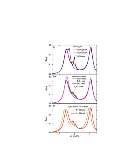
Figure 1: The HEOM calculated spectral function of an SIAM system, $A(\omega)=A_{\uparrow}(\omega)=A_{\downarrow}(\omega)$, in unit of $(\pi\Gamma)^{-1}$. The parameters adopted are specified in the caption of Table 1. The three panels exhibit the variations of $A(\omega)$, particularly the evolution of the Kondo and Hubbard peaks, versus (a) the applied bias voltage $V_{0}$, (b) the temperature $T$, and (c) the shift of impurity level energy $\epsilon$ by a gate voltage, respectively.

Figure 1 depicts the HEOM calculated spin-$\mu$ spectral function of the impurity,

$$A_{\mu}(\omega)=\frac{1}{\pi}\,{\rm Re}\left\{\int_{0}^{\infty}\!\!dt\,e^{i\omega t}\left\langle\left\{\hat{a}_{\mu}(t),\hat{a}^{\dagger}_{\mu}(0)\right\}\right\rangle_{\rm st}\,\right\}.$$ (30)

The effect of bias voltage $V_{0}$ on $A_{\mu}(\omega)$ is illustrated in Fig. 1(a). Clearly, the equilibrium $A_{\mu}(\omega)$ reproduces correctly the well known features of SIAM, such as the Hubbard peaks at around $\omega=\epsilon$ and $\omega=\epsilon+U$, and the Kondo peak centered at $\omega=\mu^{\rm eq}=0$.Hew93 In Ref. Li12266403, , the equilibrium $A_{\mu}(\omega)$ of SIAM in the Kondo regime has been investigated with the HEOM approach thoroughly and the existence of Kondo resonance is manifested by the correct universal scaling behavior there. In the nonequilibrium situation where an external voltage is applied antisymmetrically to the L and R reservoirs, the Hubbard peaks remain largely unchanged in both position and height. In contrast, the Kondo peak is split by the voltage into two, which appear at $\omega=\frac{V_{0}}{2}$ and $\omega=-\frac{V_{0}}{2}$ and correspond to the shifted reservoir chemical potentials $\mu_{\rm L}$ and $\mu_{\rm R}$, respectively. Obviously, as the bias voltage $V_{0}$ increases from $0$ to $0.2\,$meV, then to $0.7\,$meV, the progressive splitting of Kondo peak is observed in Fig. 1(a). Figure 1(b) plots the calculated $A(\omega)$ of the same SIAM system at various temperatures. Apparently, as the temperature increases over an order of magnitude, the two Hubbard resonance peaks at $\omega=\epsilon$ and $\omega=\epsilon+U$ almost remain intact. In contrast, the split peaks at $\omega=\mu_{L}$ and $\mu_{R}$ vanish quickly at the higher temperature. This clearly highlights the strong electron correlation features in the present nonequilibrium SIAM. To further verify that the split peaks near $\omega=0$ are of Kondo nature, we examine the variation of $A(\omega)$ versus a gate voltage applied to the dot. The gate voltage is considered to shift the impurity level energy $\epsilon$ by $0.1\,$meV, and the corresponding change of calculated $A(\omega)$ is shown in Fig. 1(c). Apparently, as $\epsilon$ drops from $-0.5$ to $-0.6\,$meV by the gate voltage, the two Hubbard resonance peaks at $\omega=\epsilon$ and $\omega=\epsilon+U$ are displaced by $0.1\,$meV. In contrast, the two peaks at $\omega=\pm\frac{V_{0}}{2}$ remain pinned to the reservoir chemical potentials $\mu_{L}$ and $\mu_{R}$, indicating that these two peaks are indeed of Kondo origin.

Usually, the Hubbard peaks at $\omega=\epsilon$ and $\omega=\epsilon+U$ converge more rapidly than the resonance peaks at $\omega=\pm\frac{V_{0}}{2}$ when truncation level $L$ increases. This also reflects the Kondo nature of resonance peaks at $\omega=\pm\frac{V_{0}}{2}$.SM_skw Moreover, there is a long-time oscillatory tail in the real time evolution which is crucial for the appearance of Kondo peaks. We also find that the short-time dynamics of the retarded Green’s function and high-frequency part of $A(\omega)$ converge more rapidly when the truncation level $L$ increases. In other words, in the HEOM framework, one can extract the spectral function at high frequency range at a relatively lower truncation level and relatively shorter evolution time than those at resonance frequencies, without compromising the accuracy.

We then exemplify the numerical tractability of HEOM approach via evaluation of three types of response properties. These include the local charge fluctuation spectrum $S_{Q}(\omega)$, local magnetic susceptibility $\chi_{M}(\omega)$, and differential admittance spectrum $G_{\alpha\alpha^{\prime}}(\omega)$, defined respectively as follows,

$$S_{Q}(\omega) \equiv\int^{\infty}_{-\infty}dt\,e^{i\omega t}\big{\langle}\big{\{}\Delta\hat{Q}(t),\Delta\hat{Q}(0)\big{\}}\big{\rangle}_{\rm st}\,,$$ (31)

$$\chi_{M}(\omega) \equiv i\int_{0}^{\infty}dt\,e^{i\omega t}\,\big{\langle}\big{[}\hat{M}(t),\hat{M}(0)\big{]}\big{\rangle}_{\rm st}\,,$$ (32)

$$G_{\alpha\alpha^{\prime}}(\omega) \equiv-i\int_{0}^{\infty}dt\,e^{i\omega t}\,\big{\langle}\big{[}\hat{I}_{\alpha}(t),\hat{N}_{\alpha^{\prime}}(0)\big{]}\big{\rangle}_{\rm st}\,.$$ (33)

In Eq. (31), $\Delta\hat{Q}(t)=\hat{Q}(t)-\langle\hat{Q}\rangle_{\rm st}$, with $\hat{Q}=\sum_{\mu}\hat{n}_{\mu}$ being the total impurity occupation number operator. Therefore, $\Delta\hat{Q}(t)$ describes the fluctuation of occupation number around the averaged value. For $\chi_{M}(\omega)$ of Eq. (32), $\hat{M}=g\mu_{B}\hat{S}_{z}$ is the impurity magnetization operator, which originates from the electron spin polarization induced by external magnetic field. Here, $g$ is the electron $g$-factor, $\mu_{B}$ is the Bohr magneton, and $\hat{S}_{z}=(\hat{n}_{\uparrow}-\hat{n}_{\downarrow})/2$ is the impurity spin polarization operator. In Eq. (33), $G_{\alpha\alpha^{\prime}}(\omega)$ is just the half-Fourier transform of current-number response function of Eq. (25) or (28). The time $t=0$ in the individual Eqs. (31)–(33) represents the instant at which the external perturbation (magnetic field or bias voltage) is interrogated.

It is worth pointing out that all the three types of response properties satisfy the following symmetry: the real (imaginary) part is an even (odd) function of $\omega$. This is due to the time-reversal symmetry of steady-state correlation functions, i.e., $C_{AB}(t)=[C_{BA}(-t)]^{\ast}$. In particular, for $S_{Q}(\omega)$ of Eq. (31), $\hat{A}=\hat{B}=\Delta\hat{Q}$. Consequently, it can be shown that $S_{Q}(\omega)$ is a real function. For clarity, Figs. 2, 3, and 5 will only exhibit the $\omega\geq 0$ part of the dynamic response properties, while the $\omega<0$ part can be retrieved easily by applying the symmetry relation.

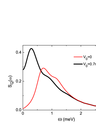
Figure 2: HEOM calculated local charge fluctuation spectrum, $S_{Q}(\omega)$ of Eq. (31), in unit of $e^{2}$. The parameters adopted are the same as those specified in caption of Table 1.

The local charge fluctuation spectrum $S_{Q}(\omega)$ has been studied in the context of shot noise of quantum dot systems.Agu04206601 ; Fli05411 ; Luo07085325 Figure 2 depicts the HEOM calculated $S_{Q}(\omega)$ of the SIAM under our investigation. At equilibrium, the spectrum exhibits a crossover behavior, where the two peaks centered at around $\omega=|\epsilon|=0.5$ meV and $\omega=|\epsilon+U|=1$ meV largely overlap and form a broad peak. The positions of these two peaks correspond to the excitation energies associated with change of impurity occupancy state. In nonequilibrium situation, the crossover peak is observed to move to a lower energy, since the chemical potential of reservoir R is drawn closer to the impurity state by the applied voltage.

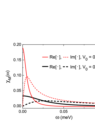
Figure 3: HEOM calculated local magnetic susceptibility, $\chi_{M}(\omega)$ of Eq. (32), in unit of $g^{2}\mu^{2}_{B}/k_{B}T$. The parameters adopted are the same as those specified in caption of Table 1.

The local magnetic susceptibility $\chi_{M}(\omega)$ is a response property of fundamental significance, particularly for strongly correlated quantum impurity systems. It has been studied by various methods such as NRG.Mer12075153 Figure 3 displays the HEOM calculated $\chi_{M}(\omega)$ of the SIAM of our concern. In both equilibrium and nonequilibrium situations, the main characteristic features of $\chi_{M}(\omega)$ appear at around zero energy. Moreover, the magnitude of $\chi_{M}(\omega)$ is found to reduce significantly in presence of applied bias voltage, especially in the low energy range. This is consistent with the diminishing spectral density at around zero-frequency due to the voltage-induced splitting of Kondo peak; see Fig. 1.

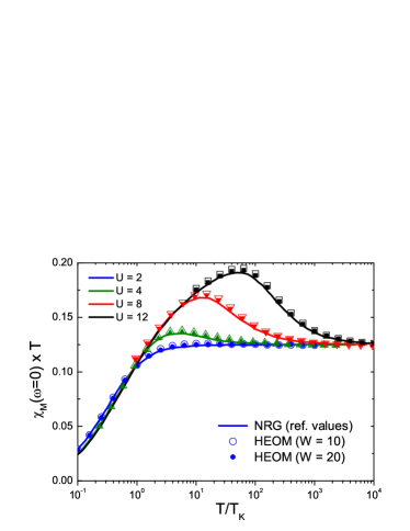
Figure 4: Static local magnetic susceptibility multiplied by temperature, $\chi_{M}(\omega=0)\,T$ (in unit of $g^{2}\mu^{2}_{B}/k_{B}$), versus $T/T_{K}$ for a series of equilibrium symmetric SIAM systems of different $U$. Here, $T_{K}$ is the Kondo temperature, and $U$, $T$, and $W$ are in unit of $\Gamma$. The HEOM results (scattered symbols) are compared with the latest full density matrix NRG calculations (lines) of Ref. Mer12075153, , the Fig. 6 there. The NRG calculations are for very large reservoir bandwidth $W$, while the HEOM results are obtained with relatively smaller bandwidths ($W=10$ and $W=20$) for saving computational cost.

To verify the numerical accuracy of our calculated local magnetic susceptibility, we compare the HEOM approach with the latest high-level NRG method. The comparison is shown in Fig. 4, where the equilibrium static magnetic susceptibilities, $\chi_{M}(\omega=0)$, of various symmetric SIAM systems are calculated to reproduce the Fig. 6 of Ref. Mer12075153, . Apparently, the HEOM and NRG results agree quantitatively with each other.

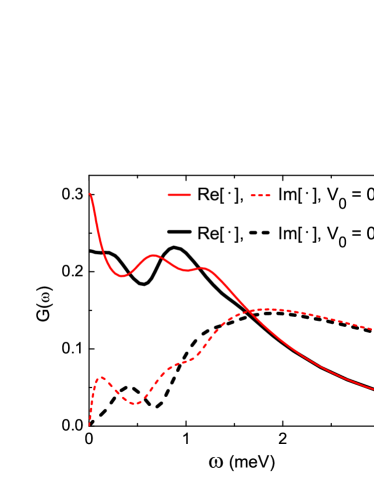
Figure 5: HEOM calculated dynamic admittance, $G(\omega)=\frac{1}{4}[G_{\rm LL}(\omega)+G_{\rm LR}(\omega)-G_{\rm RL}(\omega)-G_{\rm RR}(\omega)]$ with $G_{\alpha\alpha^{\prime}}(\omega)$ defined by Eq. (33), in unit of $e^{2}/h$. The parameters adopted are the same as those specified in caption of Table 1.

The dynamic admittance is one of the most extensively studied response properties of quantum dot systems. The frequency-dependent admittance has been studied by scattering theoryBut93364 ; But934114 ; Pre968130 ; But964793 and nonequilibrium Green’s function method.Win938487 ; Jau945528 ; Ana957632 ; Nig06206804 ; Wan07155336 The HEOM approach has also been used to calculate the dynamic admittance of noninteractingZhe08184112 and interacting quantum dots.Zhe08093016 ; Zhe09124508 This was realized by calculating the transient current in response to a delta-pulse voltage.Zhe08184112 In the following, we revisit the evaluation for dynamic admittance $G(\omega)$ via an alternative route, i.e., by calculating the current-number response functions of Eq. (25).

Figure 5 depicts the HEOM calculated differential admittance of the SIAM under study, $G(\omega)=\frac{1}{4}[G_{\rm LL}(\omega)+G_{\rm LR}(\omega)-G_{\rm RL}(\omega)-G_{\rm RR}(\omega)]=\frac{1}{2}[G_{L}(\omega)-G_{R}(\omega)]$; cf. Eq. (20), with $G_{\alpha\alpha^{\prime}}(\omega)$ defined by Eq. (33). Here we have chosen antisymmetrically applied probe ac bias, $\delta\Delta_{L}(t)=-\delta\Delta_{R}(t)=\frac{1}{2}\delta\Delta(t)$. As discussed extensively in Ref. Zhe09164708, , the characteristic features of $G(\omega)$ appearing at around $\omega=|\epsilon|$ and $\omega=|\epsilon+U|$ correspond to the transitions between Fock states of different occupancy, while the low-frequency features highlight the presence of dynamic Kondo transition. Apparently, the dynamic Kondo transition is suppressed by the applied voltage, which is analogous to the scenario of $\chi_{M}(\omega)$ as shown in Fig. 3.

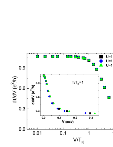
Figure 6: Calculated differential conductance $dI/dV$ of various symmetric SIAMs as a function of scaled voltage $V/T_{K}$. Here, $T_{K}$ is the Kondo temperature calculated by $T_{K}=\frac{1}{2}\sqrt{\Gamma U}\,{\rm exp}(-\pi U/4\Gamma+\pi\Gamma/4U)$, with $\Gamma=\Gamma_{L}+\Gamma_{R}$. Systems of three different combinations of parameters $U$ and $\Gamma$ (in units of meV) are demonstrated, with $T/T_{K}=1$ and $\Gamma_{L}=\Gamma_{R}$. The inset depicts $dI/dV$ versus unscaled voltage. The bandwidths of electrodes are $W_{\rm L}=W_{\rm R}=10\,$meV.

At last we investigate the universal scaling properties of nonequilibrium differential conductance $dI/dV$ (or the zero-frequency admittance). The universal scaling relation of nonequilibrium properties of impurity systems with Kondo correlations have been studied. Kam008154 ; Ros01156802 ; Pus04R513 For instance, Rosch et al. have concluded that the nonequilibrium conductance at high voltages scales universally with $V/T_{K}$; see the inset of Fig. 1 in Ref. Ros01156802, . To demonstrate the high accuracy of our HEOM approach in regimes far from equilibrium, we calculate the conductance of various symmetric SIAMs versus scaled and unscaled voltages, as displayed in Fig. 6. Clearly, while the difference in $dI/dV$–$V$ becomes more accentuated at a larger $V$ (see the inset of Fig. 6), the $dI/dV$–$V/T_{K}$ exhibits a universal scaling relation for systems of different parameters. Such a universal relation holds for all voltages examined (up to $V/T_{K}=30$). Therefore, the HEOM approach reproduces quantitatively the previously predicted universal scaling relation for nonequilibrium conductance at high voltages.

V Concluding remarks

In this work, we develop a hierarchical dynamics approach for evaluation of nonequilibrium dynamic response properties of quantum impurity systems. It is based on a hierarchical equations of motion formalism, in conjunction with a linear response theory established in the hierarchical Liouville space. It provides a unified approach for arbitrary response and correlation functions of local impurity systems, and transport current related response properties.

The proposed hierarchical Liouville-space approach resolves nonperturbatively the combined effects of e-e interactions, impurity-reservoir dissipation, and non-Markovian memory of reservoirs. It provides a unified formalism for equilibrium and nonequilibrium dynamic response properties of quantum impurity systems and can be applied to more complex quantum impurity systems without extra derivation efforts. Moreover, the HEOM results converge rapidly and uniformly with higher-tier ADOs included explicitly and one can often obtain convergent results at a relative low truncation level $L$. With our present code and the computational resources at our disposal, the lowest temperature that can be quantitatively accessed is $T\simeq 0.1\,T_{K}$ for a symmetric SIAM.

For equilibrium properties, our HEOM approach has achieved the same level of accuracy as the latest state-of-the-art NRG method.Li12266403 In this work, the accuracy of HEOM approach for calculations of nonequilibrium properties is validated by reproducing some known numerical results or analytic relations,Mer12075153 ; Ros01156802 ; Mei932601 ; Kon02125304 such as the static local magnetic susceptibility, and the universal scaling relation of high-voltage conductance.

In conclusion, the developed hierarchical Liouville-space approach provides an accurate and universal tool for investigation of general dynamic response properties of quantum impurity systems. In particular, it addresses the nonequilibrium situations and resolves the full frequency dependence details accurately. It is thus potentially useful for exploration of quantum impurity systems and strongly correlated lattice systems (combined with dynamical mean field theory), which are of experimental significance for the advancement of nanoelectronics, spintronics, and quantum information and computation.

Appendix A

In this Supplemental Material, we will discuss some details of the numerical implementation of the proposed HEOM formalism to the nonequilibrium dynamical properties of quantum impurity systems.

$L,M$	$P_{\mu}$	$P_{\uparrow\downarrow}$	$\ \bar{I}$ (nA)
1, 9	0.500 (0.500)	0.001 (0.000)	0.003
2, 9	0.441 (0.462)	0.025 (0.027)	4.654
3, 9	0.439 (0.454)	0.024 (0.025)	4.920
4, 9	0.440 (0.457)	0.024 (0.024)	4.799
4, 10	0.440 (0.457)	0.0237 (0.024)	4.805
4, 11	0.440 (0.457)	0.0237 (0.0238)	4.806
5, 9	0.440 (0.457)	0.024 (0.024)	4.799
5, 10	0.440 (0.457)	0.0237 (0.024)	4.805
5, 11	0.440 (0.457)	0.0237 (0.0238)	4.806

Table 2: Spin-$\mu$ single- and double-occupation probabilities ($P_{\mu}$ and $P_{\uparrow\downarrow}$), and steady-state current of an SIAM with two electrons reservoirs under an antisymmetrically applied bias voltage of $V_{0}=-V=0.7\,$meV. Calculations are done by solving the HEOM truncated at different level $L$ with different number of exponential terms $M$. The parameters are the same as those specified in caption of Table I of the main text. For comparison, the numbers of equilibrium situation of $V_{0}=0$ are shown in the parentheses.

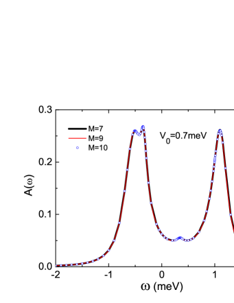
Figure 7: The convergence behavior of HEOM calculated spectral function $A(\omega)$ of SIAM (in unit of $1/\pi\Gamma$) with respect to the number of exponential terms $M$ in spectrum decomposition. Here the truncation level is fixed at $L=4$. The parameters are the same as those specified in caption of Table I of the main text.

(i) In the main text, the spectral function of $\alpha$-reservoir assumes a diagonal and Lorentzian form, i.e., $J_{\alpha\mu\nu}(\omega)=\delta_{\mu\nu}\frac{\Gamma_{\alpha}W^{2}_{\alpha}}{(\omega-\mu_{\alpha})^{2}+W^{2}_{\alpha}}$, with $\Gamma_{\alpha}$ and $W_{\alpha}$ being the linewidth and bandwidth parameters, respectively. Then in the contour integration evaluation of $\tilde{C}^{\sigma;{\rm st}}_{\alpha\mu\nu}(t)=\int_{-\infty}^{\infty}\!d\omega\frac{e^{\sigma i\omega t}J^{\sigma}_{\alpha\mu\nu}(\omega-\mu_{\alpha})}{1+e^{\sigma\beta(\omega-\mu_{\alpha})}}$, a total number of $M=N+1$ poles will be involved, including one Drude pole of the reservoir spectral density and $N$ poles of the Fermi distribution function.

In general, the number $K$ of distinct ADO indexes in the HEOM proposed in the main text amounts to $K=2N_{\alpha}N_{\mu}M$, with $N_{\mu}$ being the number spin-orbitals of system in direct contact to leads. The factor 2 accounts for the two choices of the sign variable $\sigma$, while $N_{\alpha}=2$ for the distinct $\alpha=$ L and R leads.

We have known the fact that overall computational cost increases dramatically with both $L$ and $K$. To minimize the computational cost while maintaining the quantitative accuracy, a highly efficient reservoir spectrum decomposition scheme is needed to optimize the size of $K$. Various decomposition schemes have been developed, including Matsubara spectrum decomposition,Jin08234703 partial fractional decomposition, Cro09073102 Padé spectrum decomposition (PSD), Hu10101106 ; Hu11244106 and hybrid scheme.Zhe09164708 To our knowledge, PSD scheme has the best performance and acquires the same accuracy with the minimal size of $K$ until now. In the present work, the $[N\!-\!1/N]$ Padé spectrum decomposition schemeHu10101106 ; Hu11244106 is used for the efficient construction of the hierarchical Liouville propagator.

There is an overlap between Fermi distribution function $f^{(\sigma)}_{\alpha}(\omega-\mu_{\alpha})$ and bath spectral density $J^{\sigma}_{\alpha\mu\nu}(\omega-\mu_{\alpha})$ in the definition of bath correlation function $\tilde{C}^{\sigma;{\rm st}}_{\alpha\mu\nu}(t)=\int_{-\infty}^{\infty}\!d\omega e^{\sigma i\omega t}f^{(\sigma)}_{\alpha}(\omega-\mu_{\alpha})J^{\sigma}_{\alpha\mu\nu}(\omega-\mu_{\alpha})$. Due to the finite bandwidth of reservoirs in realistic quantum impurity system, the residual between $f^{(\sigma)}_{\alpha}(\omega-\mu_{\alpha})$ and its Padé series expansion (with large enough $N$) at $\omega\gg W_{\alpha}$ will not introduce any approximation. Therefore, the exponential series expansion of bath correlation function with large enough $M$ can efficiently resolves the non-Markovian memory of reservoirs in both equilibrium and nonequilibrium situations.

To obtain quantitatively accurate numerical results, we increase the number of exponential terms $M$ in spectrum decomposition continually until convergent results are arrived in practice.Li12266403

Table 2 lists the probabilities that the impurity is singly occupied by spin-$\mu$ electron ($P_{\mu}=\langle\mu|\bar{\rho}(T,V)|\mu\rangle$ with $\mu=\uparrow$ or $\downarrow$); or doubly occupied ($P_{\uparrow\downarrow}=\langle{\uparrow\downarrow}|\bar{\rho}(T,V)|{\uparrow\downarrow}\rangle$). Here, $\bar{\rho}(T,V)$ is the nonequilibrium steady-state reduced density matrix under temperature $T$ and antisymmetric applied voltage $V$. Calculations are done at different truncation level $L$ and different number of exponential terms $M$ (up to $L=5$ and $M=11$). Apparently, the HEOM results converge rapidly with the increasing $L$, i.e., with higher-tier ADOs included explicitly in HEOM. In particular, the remaining relative deviations between the results of $L=4$ and $L=5$ are less than 0.1%, indicating that the $L=4$ level of truncation is sufficient for the present set of parameters. At the same time, one can observe that $M=9$ is sufficient to yield convergent results here. These are further affirmed by the calculated steady-state current $\bar{I}(V)$ across the impurity, which also converges quantitatively with rather minor residual uncertainty at $L=4$ and $M=9$.

Fig. 7 further illustrates the convergence behavior of $A(\omega)$ of SIAM with respect to the number of exponential terms $M$ at the fixed truncation level $L=4$. Obviously $M=9$ is large enough for the adopted parameters of the numerical examples in the main text.

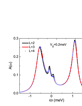
Figure 8: The convergence behavior of HEOM calculated spectral function $A(\omega)$ of SIAM (in unit of $1/\pi\Gamma$) with respect to the truncation level $L=2,3,4$ with the fixed number of exponential terms $M=9$. The parameters are the same as those specified in caption of Table I of the main text.

(ii) The terminal truncation level $L_{max}$ is often too high to reach in practical implementation, and a truncation at a relatively low level $L$ is inevitable. Here we adopt a straightforward truncation scheme, i.e., set all the higher-tier ADOs ($n>L$) zero directly. And we increase the truncation level $L$ continually until the convergent numerical results are obtained. For quantum impurity systems with nonzero e-e interactions, calculations often converge rapidly and uniformly with the increasing truncation level $L$. For weak to medium system-reservoir coupling strength, one can often obtain quantitatively accurate results at a relatively low $L$. HEOM calculated spectral function $A(\omega)$ of SIAM at different truncation level $L=2$, $3$, $4$ with the fixed number of exponential terms in spectrum decomposition ($M=9$) are plotted together in Fig. 8, to illustrate the convergence behavior and gain the feeling on the numerical aspects of the proposed formalism. Obviously, the numerical results converge rapidly and uniformly with the increasing truncation level $L$. Fig. 8 further confirms the fact that $L=4$ level of truncation is sufficient for the set of parameters adopted in the main text. One can also observe that the resonance Hubbard peaks at around $\omega=\epsilon$ and $\omega=\epsilon+U$ converge more easily than the split Kondo peaks at $\omega=\pm\frac{V_{0}}{2}$ with increasing truncation level $L$. This further confirms the strong correlation nature of resonance at $\omega=\pm\frac{V_{0}}{2}$. Moreover, the numerical results at high and far-from-resonance frequency range converge more easily than those at Kondo resonance frequencies.

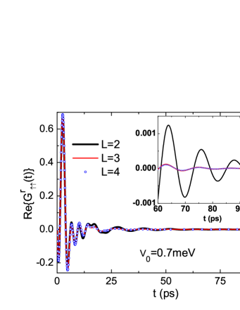
Figure 9: The convergence behavior of HEOM calculated $G^{r}_{\uparrow\uparrow}(t>0)$ of SIAM with respect to the truncation level $L=2,3,4$, with fixed $M=9$. The parameters are the same as those specified in caption of Table I of the main text. The inset magnifies the long time oscillatory tail in real time evolution.

(iii) The hierarchical Liouville-space linear response theory proposed in the main text can be implemented in either time-domain or frequency domain. In the time-domain scheme, one first carry out the real-time evolution under the unperturbed HEOM propagator ${\mbox{\boldmath${\cal G}$}}_{s}(t)$, starting from the initial condition $\tilde{\bm{\rho}}(0)$, i.e.,

$$\tilde{\bm{\rho}}(t)={\mbox{\boldmath${\cal G}$}}_{s}(t)\tilde{\bm{\rho}}(0).$$ (34)

Then the correlation/response functions can be extracted from certain ADOs components $\{\tilde{\rho}^{(n)}_{j_{1}...j_{n}}\!(t)\}$ in $\tilde{\bm{\rho}}(t)$, as in Eq. (20) of the main text. At last the frequency-dependent dynamical properties are obtained straightforwardly by a half Fourier transform.

Fig. 9 depicts the HEOM calculated real part of $G^{r}_{\uparrow\uparrow}(t>0)=-\frac{i}{\hbar}\langle\{\hat{a}_{\uparrow}(t),\hat{a}^{\dagger}_{\uparrow}(0)\}\rangle_{\rm st}$ of SIAM system at different truncation level $L=2$, $3$, $4$. The number of exponential terms in spectrum decomposition is fixed at $M=9$. The imaginary part of $G^{r}_{\uparrow\uparrow}(t>0)$ has the same convergence behavior and is ignored here.

Obviously the short-time dynamics converges more easily than long-time dynamics when the truncation level $L$ increases. This is consistent with the frequency-domain convergence features with respect to truncation level indicated in Fig. 8. This is because that dynamical properties at high and far-from-resonance frequency range are dominated by the short-time evolution.

As illustrated in the inset of Fig. 9, the real time evolution has a long-time oscillatory tail. To obtain quantitative accurate spectral function at high and off-resonant frequencies, one only need evolve relative short time $t$. In contrast, the accurate Kondo peaks can be achieved only when long enough oscillatory evolution is included. Therefore the long-time oscillatory tail is crucial for the Kondo resonance peaks. It can be viewed as another evidence of the existence of Kondo correlation.

Therefore for strongly correlated quantum impurity systems at low temperatures, where Kondo signatures appear at the position of chemical potentials $\mu_{\alpha}$, one must propagate $G^{r}_{\uparrow\uparrow}(t>0)$ to a long enough time to include the significant long-time memory of reservoir. Consequently, it is very time-consuming to obtain quantitative accuracy at the frequencies of Kondo peaks. For the present parameters in the main text, when $V_{0}=0.7\,$meV, $L=4$ and $M=9$, the time evolution needs to be extended over $190\,$ps (costing $10000$ minutes of CPU time) to obtain accurate Kondo peaks.

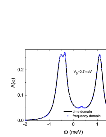
Figure 10: HEOM calculated spectral function $A(\omega)$ of SIAM obtained in both time domain with $t=190\,$ps and frequency domain, in unit of $(\pi\Gamma)^{-1}$. The parameters are the same as those specified in Fig. 9. The truncation level is fixed at $L=4$ and the number of exponential terms in spectrum decomposition is fixed at $M=9$.

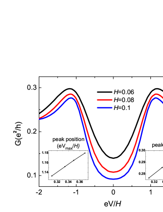
Figure 11: Calculated differential conductance $G=dI/dV$ of a symmetrical SIAM under magnetic fields of different magnitudes ($H$). The other parameters adopted are (in meV): $\Gamma=\Gamma_{\rm L}=\Gamma_{\rm R}=0.1$, $\epsilon=\epsilon_{\uparrow}=\epsilon_{\downarrow}=-0.6$, $U=1.2$, $W_{\rm L}=W_{\rm R}=2$, and $T=0.01$. The insets display the variations of peak position $eV_{\rm max}/H$ and peak height with respect to $[\ln(H/(2T_{K})\sqrt{\pi e/2})]^{-1}$, respectively. Here, the Kondo temperature is evaluated as $T_{K}=\sqrt{\Gamma U/2}\,e^{\,\pi[\epsilon(\epsilon+U)+\Gamma^{2}]/(2\Gamma U)}\approx 0.002508\,$meV.

An alternative numerical scheme is carried out in frequency domain. In frequency-domain scheme one solves the following sparse linear algebra problem at a fixed frequency $\omega$,

$$-i\omega\tilde{\rho}^{(n)}_{j_{1}\cdots j_{n}}(\omega)-\tilde{\rho}^{(n)}_{j_{1}\cdots j_{n}}(0)=-\big{[}i\mathcal{L}_{s}+\sum_{r=1}^{n}\gamma_{j_{r}}\big{]}\tilde{\rho}^{(n)}_{j_{1}\cdots j_{n}}(\omega)$$

$$-i\sideset{}{{}^{\prime}}{\sum}_{j}{\cal A}_{\bar{j}}\,\tilde{\rho}^{(n+1)}_{j_{1}\cdots j_{n}j}(\omega)-i\sum_{r=1}^{n}(-)^{n-r}\,{\cal C}_{j_{r}}\,\tilde{\rho}^{(n-1)}_{j_{1}\cdots j_{r-1}j_{r+1}\cdots j_{n}}(\omega)\,.$$ (35)

where $\tilde{\rho}^{(n)}_{j_{1}\cdots j_{n}}(\omega)$ is the half-Fourier transformation of $\tilde{\rho}^{(n)}_{j_{1}\cdots j_{n}}(t)$. And $\tilde{\rho}^{(n)}_{j_{1}\cdots j_{n}}(0)$ is the initial condition of the corresponding correlation/response function. To obtain the whole spectrum, a full scan for the whole frequency domain is needed.

The equivalence between the time- and frequency-domain schemes is exemplified with Fig. 10, where the spectral function $A(\omega)$ of a SIAM is calculated with both time- and frequency-domain schemes. Apparently, the results of both schemes agree perfectly with each other.

In practice, one can employ a hybrid time- and frequency-domain scheme. The overall profile can be plotted with the time-domain scheme, while the detailed structures of the resonance and Kondo peaks can be exploited with the frequency-domain scheme. This hybrid scheme provides an accurate and efficient method to calculate the full spectrum of a strongly correlated quantum impurity system in the Kondo regime.

We then investigate the effects of external magnetic field on the static differential conductance of an SIAM system in the Kondo regime. The magnetic field causes the Zeeman splitting for the impurity level through an additional interaction Hamiltonian of $\hat{H}_{\rm M}=-H\hat{S}_{z}$. The effects of the magnetic field on the nonequilibrium properties of the SIAM, such as the steady-state differential conductance ($G\equiv dI/dV$), have been explored in the literature.Mei932601 ; Kon01236801 ; Kon02125304 Konik, Saleur, and LudwigKon02125304 have analyzed the asymptotic behavior of the peak position ($eV_{\rm max}/H$) and peak height with increasing $H$ –they vary logarithmically in $H$. Taking the peak position as an example, it has been found that as $H/T_{K}\rightarrow\infty$,Kon02125304

$$\frac{eV_{\rm max}}{H}\propto\left[\ln\left(\frac{H}{2T_{K}}\sqrt{\frac{\pi e}{2}}\right)\right]^{-1}.$$ (36)

Figure 11 depicts the calculated $G$ versus $eV/H$ for various values of $H(\gg T_{K})$. Here, $\mu_{L}$ is fixed at its equilibrium value, while $\mu_{R}$ is shifted by the applied bias voltage. In contrast to Ref. Kon02125304, where zero temperature is considered, the HEOM calculations are done at a low but finite temperature, $T=0.01\,$meV, because of our limited computational resources. The insets of Fig. 11 show clearly that both $eV_{\rm max}/H$ and peak height indeed vary linearly with respect to the quantity at the right-hand side of Eq. (36). Moreover, by linear extrapolation to $H\rightarrow\infty$, the ratio $eV_{\rm max}/H$ approaches a value of around $0.88$, smaller than $1$. Therefore, different from the $T=0$ case where $eV_{\rm max}/H$ is always smaller than $1$, our calculations indicate that, at a finite temperature such a ratio may decrease from above $1$ to a value smaller than $1$. Such a trend has been observed experimentally; see for instance, Fig. 4(b) of Ref. Cro98540, .

In summary, the truncation level and the number of exponential terms in spectrum decomposition are continuously increased until convergent numerical results are obtained. Therefore the proposed HEOM nonequilibrium linear response theory provides an quantitatively accurate numerical tool for arbitrary response and correlation functions of local impurity systems, and transport related response properties. In the frame of our HEOM formalism, one can extract dynamical properties at high and off-resonant frequency range at relative lower truncation level and relative shorter evolution time than those at resonance frequencies, maintaining quantitative accuracy. The hybrid time- and frequency-domain scheme provides an accurate and efficient method to obtain the full spectrum of a quantum impurity system in the Kondo regime.

References

- (1) J. M. Elzerman, R. Hanson, L. H. Willems van Beveren, B. Witkamp, L. M. K. Vandersypen, and L. P. Kouwenhoven, Nature 430, 431 (2004).
- (2) F. H. L. Koppens, C. Buizert, K. J. Tielrooij, I. T. Vink, K. C. Nowack, T. Meunier, L. P. Kouwenhoven, and L. M. K. Vandersypen, Nature 442, 766 (2006).
- (3) R. Hanson and D. D. Awschalom, Nature 453, 1043 (2008).
- (4) J. Gabelli, G. Fève, J. -M. Berroir, B. Plaçais, A. Cavanna, B. Etienne, Y. Jin, and D. C. Glattli, Science 313, 499 (2006).
- (5) G. Fève, A. Mahé, J. -M. Berroir, T. Kontos, B. Plaçais, D. C. Glattli, A. Cavanna, B. Etienne, and Y. Jin, Science 316, 1169 (2007).
- (6) W. Metzner and D. Vollhardt, Phys. Rev. Lett. 62, 324 (1989).
- (7) A. Georges and G. Kotliar, Phys. Rev. B 45, 6479 (1992).
- (8) A. Georges, G. Kotliar, W. Krauth, and M. J. Rozenberg, Rev. Mod. Phys. 68, 13 (1996).
- (9) S. M. Cronenwett, T. H. Oosterkamp, and L. P. Kouwenhoven, Science 281, 540 (1998).
- (10) D. Goldhaber-Gordon, H. Shtrikman, D. Mahalu, D. Abusch-Magder, U. Meirav, and M. A. Kastner, Nature 391, 156 (1998).
- (11) R. Bulla, T. A. Costi, and T. Pruschke, Rev. Mod. Phys. 80, 395 (2008).
- (12) A. Georges and W. Krauth, Phys. Rev. Lett. 69, 1240 (1992).
- (13) M. Imada, A. Fujimori, and Y. Tokura, Rev. Mod. Phys. 70, 1039 (1998).
- (14) R. Bulla, T. A. Costi, and D. Vollhardt, Phys. Rev. B 64, 045103 (2001).
- (15) V. J. Emery, Phys. Rev. Lett. 58, 2794 (1987).
- (16) Y. Yanase, T. Jujo, T. Nomura, H. Ikeda, T. Hotta, and K. Yamada, Phys. Rep. 387, 1 (2003).
- (17) T. A. Maier, M. Jarrell, T. C. Schulthess, P. R. C. Kent, and J. B. White, Phys. Rev. Lett. 95, 237001 (2005).
- (18) K. G. Wilson, Rev. Mod. Phys. 47, 773 (1975).
- (19) W. Hofstetter, Phys. Rev. Lett. 85, 1508 (2000).
- (20) S. R. White, Phys. Rev. Lett. 69, 2863 (1992).
- (21) E. Jeckelmann, Phys. Rev. B 66, 045114 (2002).
- (22) S. Nishimoto and E. Jeckelmann, J. Phys.: Condens. Matter 16, 613 (2004).
- (23) J. E. Hirsch and R. M. Fye, Phys. Rev. Lett. 56, 2521 (1986).
- (24) R. N. Silver, D. S. Sivia, and J. E. Gubernatis, Phys. Rev. B 41, 2380 (1990).
- (25) J. E. Gubernatis, M. Jarrell, R. N. Silver, and D. S. Sivia, Phys. Rev. B 44, 6011 (1991).
- (26) E. Gull, A. J. Millis, A. I. Lichtenstein, A. N. Rubtsov, M. Troyer, and P. Werner, Rev. Mod. Phys. 83, 349 (2011).
- (27) B. Doyon and N. Andrei, Phys. Rev. B 73, 245326 (2006).
- (28) P. Mehta and N. Andrei, Phys. Rev. Lett. 100, 086804 (2008).
- (29) E. Boulat, H. Saleur, and P. Schmitteckert, Phys. Rev. Lett. 101, 140601 (2008).
- (30) C.-H. Chung, K. Le Hur, M. Vojta, and P. Wölfle, Phys. Rev. Lett. 102, 216803 (2009).
- (31) T. A. Costi, Phys. Rev. B 55, 3003 (1997).
- (32) F. B. Anders and A. Schiller, Phys. Rev. Lett. 95, 196801 (2005).
- (33) F. B. Anders, Phys. Rev. Lett. 101, 066804 (2008).
- (34) S. R. White and A. E. Feiguin, Phys. Rev. Lett. 93, 076401 (2004).
- (35) S. G. Jakobs, V. Meden, and H. Schoeller, Phys. Rev. Lett. 99, 150603 (2007).
- (36) R. Gezzi, T. Pruschke, and V. Meden, Phys. Rev. B 75, 045324 (2007).
- (37) J. E. Han and R. J. Heary, Phys. Rev. Lett. 99, 236808 (2007).
- (38) P. Werner, T. Oka, and A. J. Millis, Phys. Rev. B 79, 035320 (2009).
- (39) M. Schiró and M. Fabrizio, Phys. Rev. B 79, 153302 (2009).
- (40) S. Weiss, J. Eckel, M. Thorwart, and R. Egger, Phys. Rev. B 77, 195316 (2008).
- (41) D. Segal, A. J. Millis, and D. R. Reichman, Phys. Rev. B 82, 205323 (2010).
- (42) R. M. Konik, H. Saleur, and A. W. W. Ludwig, Phys. Rev. Lett. 87, 236801 (2001).
- (43) P. Mehta and N. Andrei, Phys. Rev. Lett. 96, 216802 (2006).
- (44) S.-P. Chao and G. Palacios, Phys. Rev. B 83, 195314 (2011).
- (45) J. S. Jin, X. Zheng, and Y. J. Yan, J. Chem. Phys. 128, 234703 (2008).
- (46) X. Zheng, J. S. Jin, S. Welack, M. Luo, and Y. J. Yan, J. Chem. Phys. 130, 164708 (2009).
- (47) Zheng Xiao, Xu Ruixue, Xu Jian, Jin Jinshuang, Hu Jie, and Yan Yijing, Prog. Chem. 24, 1129 (2012).
- (48) Z. H. Li, N. H. Tong, X. Zheng, D. Hou, J. H. Wei, J. Hu, and Y. J. Yan, Phys. Rev. Lett. 109, 266403 (2012).
- (49) G. Stefanucci and C.-O. Almbladh, Phys. Rev. B 69, 195318 (2004).
- (50) J. Maciejko, J. Wang, and H. Guo, Phys. Rev. B 74, 085324 (2006).
- (51) X. Zheng, J. S. Jin, and Y. J. Yan, J. Chem. Phys. 129, 184112 (2008).
- (52) X. Zheng, J. S. Jin, and Y. J. Yan, New J. Phys. 10, 093016 (2008).
- (53) F. Jiang, J. S. Jin, S. K. Wang, and Y. J. Yan, Phys. Rev. B 85, 245427 (2012).
- (54) A. Croy and U. Saalmann, Phys. Rev. B 80, 073102 (2009).
- (55) J. Hu, R. X. Xu, and Y. J. Yan, J. Chem. Phys. 133, 101106 (2010).
- (56) J. Hu, M. Luo, F. Jiang, R. X. Xu, and Y. J. Yan, J. Chem. Phys. 134, 244106 (2011).
- (57) X. Zheng, J. Y. Luo, J. S. Jin, and Y. J. Yan, J. Chem. Phys. 130, 124508 (2009).
- (58) Y. Mo, R. X. Xu, P. Cui, and Y. J. Yan, J. Chem. Phys. 122, 084115 (2005).
- (59) K. B. Zhu, R. X. Xu, H. Y. Zhang, J. Hu, and Y. J. Yan, J. Phys. Chem. B 115, 5678 (2011).
- (60) J. Xu, R. X. Xu, D. Abramavicius, H. D. Zhang, and Y. J. Yan, Chin. J. Chem. Phys. 24, 497 (2011).
- (61) J. Xu, H. D. Zhang, R. X. Xu, and Y. J. Yan, J. Chem. Phys. 138, 024106 (2013).
- (62) R. X. Xu, P. Cui, X. Q. Li, Y. Mo, and Y. J. Yan, J. Chem. Phys. 122, 041103 (2005).
- (63) Q. Shi, L. P. Chen, G. J. Nan, R. X. Xu, and Y. J. Yan, J. Chem. Phys. 130, 084105 (2009).
- (64) G. A. Baker Jr. and P. Graves-Morris, Padé Approximants, Cambridge University Press, New York, 1996, 2nd ed.
- (65) See the Supplemental Material for the numerical details on the HEOM evaluation of nonequilibrium dynamical properties of quantum impurity systems.
- (66) A. C. Hewson, The Kondo Problem to Heavy Fermions, Cambridge University Press, Cambridge, 1993.
- (67) R. Aguado and T. Brandes, Phys. Rev. Lett. 92, 206601 (2004).
- (68) C. Flindt, T. Novotný, and A.-P. Jauho, Physica E 29, 411 (2005).
- (69) J. Y. Luo, X. Q. Li, and Y. J. Yan, Phys. Rev. B 76, 085325 (2007).
- (70) L. Merker, A. Weichselbaum, and T. A. Costi, Phys. Rev. B 86, 075153 (2012).
- (71) M. Büttiker, H. Thomas, and A. Prêtre, Phys. Lett. A 180, 364 (1993).
- (72) M. Büttiker, A. Prêtre, and H. Thomas, Phys. Rev. Lett. 70, 4114 (1993).
- (73) A. Prêtre, H. Thomas, and M. Büttiker, Phys. Rev. B 54, 8130 (1996).
- (74) M. Büttiker, J. Math. Phys. 37, 4793 (1996).
- (75) N. S. Wingreen, A.-P. Jauho, and Y. Meir, Phys. Rev. B 48, 8487 (1993).
- (76) A.-P. Jauho, N. S. Wingreen, and Y. Meir, Phys. Rev. B 50, 5528 (1994).
- (77) M. P. Anantram and S. Datta, Phys. Rev. B 51, 7632 (1995).
- (78) S. E. Nigg, R. López, and M. Büttiker, Phys. Rev. Lett. 97, 206804 (2006).
- (79) J. Wang, B. Wang, and H. Guo, Phys. Rev. B 75, 155336 (2007).
- (80) A. Kaminski, Y. V. Nazarov, and L. I. Glazman, Phys. Rev. B 62, 8154 (2000).
- (81) A. Rosch, J. Kroha, and P. Wölfle, Phys. Rev. Lett. 87, 156802 (2001).
- (82) M. Pustilnik and L. Glazman, J. Phys.: Condens. Matter 16, R153 (2004).
- (83) Y. Meir, N. S. Wingreen, and P. A. Lee, Phys. Rev. Lett. 70, 2601 (1993).
- (84) R. M. Konik, H. Saleur, and A. Ludwig, Phys. Rev. B 66, 125304 (2002).