The geometric mean is a Bernstein function

Abstract.

In the paper, the authors establish, by using Cauchy integral formula in the theory of complex functions, an integral representation for the geometric mean of $n$ positive numbers. From this integral representation, the geometric mean is proved to be a Bernstein function and a new proof of the well known AG inequality is provided.

1. Introduction

We recall some notions and definitions.

Definition 1.1 ([15, 26]).

A function $f$ is said to be completely monotonic on an interval $I$ if $f$ has derivatives of all orders on $I$ and

$$(-1)^{n}f^{(n)}(t)\geq 0$$ (1.1)

for $x\in I$ and $n\geq 0$.

The class of completely monotonic functions on $(0,\infty)$ is characterized by the famous Hausdorff-Bernstein-Widder Theorem below.

Proposition 1.1 ([26, p. 161, Theorem 12b]).

A necessary and sufficient condition that $f(x)$ should be completely monotonic for $0<x<\infty$ is that

$$f(x)=\int_{0}^{\infty}e^{-xt}\operatorname{d\mspace{-2.0mu}}\alpha(t),$$ (1.2)

where $\alpha(t)$ is non-decreasing and the integral converges for $0<x<\infty$.

Definition 1.2 ([18, 20]).

A function $f$ is said to be logarithmically completely monotonic on an interval $I$ if its logarithm $\ln f$ satisfies

$$(-1)^{k}[\ln f(t)]^{(k)}\geq 0$$ (1.3)

for $k\in\mathbb{N}$ on $I$.

It has been proved in [3, 8, 18, 20] that a logarithmically completely monotonic function on an interval $I$ must be completely monotonic on $I$.

Definition 1.3 ([24, 26]).

A function $f:I\subseteq(-\infty,\infty)\to[0,\infty)$ is called a Bernstein function on $I$ if $f(t)$ has derivatives of all orders and $f^{\prime}(t)$ is completely monotonic on $I$.

The class of Bernstein functions can be characterized by

Proposition 1.2 ([24, p. 15, Theorem 3.2]).

A function $f:(0,\infty)\to\mathbb{R}$ is a Bernstein function if and only if it admits the representation

$$f(x)=a+bx+\int_{0}^{\infty}\bigl{(}1-e^{-xt}\bigr{)}\operatorname{d\mspace{-2.0mu}}\mu(t),$$ (1.4)

where $a,b\geq 0$ and $\mu$ is a measure on $(0,\infty)$ satisfying

$$\int_{0}^{\infty}\min\{1,t\}\operatorname{d\mspace{-2.0mu}}\mu(t)<\infty.$$

In [5, pp. 161–162, Theorem 3] and [24, p. 45, Proposition 5.17], it was discovered that the reciprocal of any Bernstein function is logarithmically completely monotonic.

Definition 1.4 ([1]).

If $f^{(k)}(t)$ for some nonnegative integer $k$ is completely monotonic on an interval $I$, but $f^{(k-1)}(t)$ is not completely monotonic on $I$, then $f(t)$ is called a completely monotonic function of $k$-th order on an interval $I$.

It is obvious that a completely monotonic function of first order is a Bernstein function if and only if it is nonnegative on $I$.

Definition 1.5 ([24, p. 19, Definition 2.1]).

If $f:(0,\infty)\to[0,\infty)$ can be written in the form

$$f(x)=\frac{a}{x}+b+\int_{0}^{\infty}\frac{1}{s+x}{\operatorname{d\mspace{-2.0mu}}\mu(s)},$$ (1.5)

then it is called a Stieltjes function, where $a,b\geq 0$ are nonnegative constants and $\mu$ is a nonnegative measure on $(0,\infty)$ such that

$$\int_{0}^{\infty}\frac{1}{1+s}\operatorname{d\mspace{-2.0mu}}\mu(s)<\infty.$$

The set of logarithmically completely monotonic functions on $(0,\infty)$ contains all Stieltjes functions, see [3] or [22, Remark 4.8]. In other words, all the Stieltjes functions are logarithmically completely monotonic on $(0,\infty)$.

In the newly-published paper [7], a new notion “completely monotonic degree” of nonnegative functions was naturally introduced and initially studied.

We also recall that the extended mean value $E(r,s;x,y)$ may be defined as

$$E(r,s;x,y) =\biggl{[}\frac{r(y^{s}-x^{s})}{s(y^{r}-x^{r})}\biggr{]}^{{1/(s-r)}}, rs(r-s)(x-y) \neq 0;$$ (1.6)

$$E(r,0;x,y) =\biggl{[}\frac{y^{r}-x^{r}}{r(\ln y-\ln x)}\biggr{]}^{{1/r}}, r(x-y) \neq 0;$$ (1.7)

$$E(r,r;x,y) =\frac{1}{e^{1/r}}\biggl{(}\frac{x^{x^{r}}}{y^{y^{r}}}\biggr{)}^{{1/(x^{r}-y^{r})}}, r(x-y) \neq 0;$$ (1.8)

$$E(0,0;x,y) =\sqrt{xy}\,, x \neq y;$$ (1.9)

$$E(r,s;x,x) =x, x =y;$$

where $x$ and $y$ are positive numbers and $r,s\in\mathbb{R}$. Because this mean was first defined in [25], so it is also called Stolarsky’s mean. Many special mean values with two variables are special cases of $E$, for example,

$$E(r,2r;x,y) =M_{r}(x,y), (\text{power mean or H\"{o}lder mean})$$

$$E(1,p;x,y) =L_{p}(x,y), (\text{generalized or extended logarithmic mean})$$

$$E(1,1;x,y) =I(x,y), (\text{identric or exponential mean})$$

$$E(1,2;x,y) =A(x,y), (\text{arithmtic mean})$$

$$E(0,0;x,y) =G(x,y), (\text{geometric mean})$$

$$E(-2,-1;x,y) =H(x,y), (\text{harmonic mean})$$

$$E(0,1;x,y) =L(x,y). (\text{logarithmic mean})$$

For more information on $E$, please refer to the monograph [4], the papers [9, 10, 11], and closely-related references therein.

It is easy to see that the arithmetic mean

$$A_{x,y}(t)=A(x+t,y+t)=A(x,y)+t$$

is a trivial Bernstein function of $t\in(-\min\{x,y\},\infty)$ for $x,y>0$.

It is not difficult to see that the harmonic mean

$$H_{x,y}(t)=H(x+t,y+t)=\frac{2}{\frac{1}{x+t}+\frac{1}{y+t}}$$ (1.10)

for $t\in(-\min\{x,y\},\infty)$ and $x,y>0$ with $x\neq y$ meets

$$H_{x,y}^{\prime}(t)=\frac{2\bigl{[}x^{2}+y^{2}+2(x+y)t+2t^{2}\bigr{]}}{(x+y+2t)^{2}}=1+\frac{(x-y)^{2}}{(x+y+2t)^{2}}>1.$$ (1.11)

It is obvious that the derivative $H_{x,y}^{\prime}(t)$ is completely monotonic with respect to $t$. As a result, the harmonic mean $H_{x,y}(t)$ is a Bernstein function of $t$ on $(-\min\{x,y\},\infty)$ for $x,y>0$ with $x\neq y$.

In [21, Remark 6], it was pointed out that the reciprocal of the identric mean

$$I_{x,y}(t)=I(x+t,y+t)=\frac{1}{e}\biggl{[}\frac{(x+t)^{x+t}}{(y+t)^{y+t}}\biggr{]}^{{1/(x-y)}}$$ (1.12)

for $x,y>0$ with $x\neq y$ is a logarithmically completely monotonic function of $t\in(-\min\{x,y\},\infty)$ and that the identric mean $I_{x,y}(t)$ for $t>-\min\{x,y\}$ with $x\neq y$ is also a completely monotonic function of first order (that is, a Bernstein function).

In [17, p. 616], it was concluded that the logarithmic mean

$$L_{x,y}(t)=L(x+t,y+t)$$ (1.13)

is increasing and concave in $t>-\min\{x,y\}$ for $x,y>0$ with $x\neq y$. More strongly, it was proved in [19, Theorem 1] that the logarithmic mean $L_{x,y}(t)$ for $x,y>0$ with $x\neq y$ is a completely monotonic function of first order in $t\in(-\min\{x,y\},\infty)$, that is, the logarithmic mean $L_{x,y}(t)$ is a Bernstein function of $t\in(-\min\{x,y\},\infty)$.

Recently, the geometric mean

$$G_{x,y}(t)=G(x+t,y+t)=\sqrt{(x+t)(y+t)}\,$$ (1.14)

was proved in [23] to be a Bernstein function of $t$ on $(-\min\{x,y\},\infty)$ for $x,y>0$ with $x\neq y$, and its integral representation

$$G_{x,y}(t)=G(x,y)+t+\frac{x-y}{2\pi}\int_{0}^{\infty}\frac{\rho((x-y)s)}{s}e^{-ys}\bigl{(}1-e^{-st}\bigr{)}\operatorname{d\mspace{-2.0mu}}s$$ (1.15)

for $x>y>0$ and $t>-y$ was discovered, where

$$\rho(s) =\int_{0}^{1/2}q(u)\bigl{[}1-e^{-(1-2u)s}\bigr{]}e^{-us}\operatorname{d\mspace{-2.0mu}}u$$ (1.16)

$$=\int_{0}^{1/2}q\biggl{(}\frac{1}{2}-u\biggr{)}\bigl{(}e^{us}-e^{-us}\bigr{)}e^{-s/2}\operatorname{d\mspace{-2.0mu}}u$$

$$\geq 0$$

on $(0,\infty)$ and

$$q(u)=\sqrt{\frac{1}{u}-1}\,-\frac{1}{\sqrt{1/u-1}\,}$$ (1.17)

on $(0,1)$.

Let $a=(a_{1},a_{2},\dotsc,a_{n})$ for $n\in\mathbb{N}$, the set of all positive integers, be a given sequence of positive numbers. Then the arithmetic and geometric means $A_{n}(a)$ and $G_{n}(a)$ of the numbers $a_{1},a_{2},\dotsc,a_{n}$ are defined respectively as

$$A_{n}(a)=\frac{1}{n}\sum_{k=1}^{n}a_{k}$$ (1.18)

and

$$G_{n}(a)=\Biggl{(}\prod_{k=1}^{n}a_{k}\Biggr{)}^{1/n}.$$ (1.19)

It is general knowledge that

$$G_{n}(a)\leq A_{n}(a),$$ (1.20)

with equality if and only if $a_{1}=a_{2}=\dotsm=a_{n}$.

There has been a large number, presumably over one hundred, of proofs of the AG inequality (1.20) in the mathematical literature. The most complete information, so far, can be found in the monographs [2, 4, 12, 13, 14, 16] and a lot of references therein.

In this paper, we establish, by using Cauchy integral formula in the theory of complex functions, an integral representation of the geometric mean

$$G_{n}(a+z)=\Biggl{[}\prod_{k=1}^{n}(a_{k}+z)\Biggr{]}^{1/n},$$ (1.21)

where $a=(a_{1},a_{2},\dotsc,a_{n})$ satisfies $a_{k}>0$ for $1\leq k\leq n$ and

$$z\in\mathbb{C}\setminus(-\infty,-\min\{a_{k},1\leq k\leq n\}].$$

From this integral representation, it is immediately derived that the geometric mean $G_{n}(a+t)$ for $t\in(-\min\{a_{k},1\leq k\leq n\},\infty)$ is a Bernstein function, where $a+t=(a_{1}+t,a_{2}+t,\dotsc,a_{n}+t)$, and a new proof of the AG inequality (1.20) is provided.

2. Lemmas

In order to prove our main results, we need the following lemmas.

Lemma 2.1 (Cauchy integral formula [6, p. 113]).

Let $D$ be a bounded domain with piecewise smooth boundary. If $f(z)$ is analytic on $D$, and $f(z)$ extends smoothly to the boundary of $D$, then

$$f(z)=\frac{1}{2\pi i}\oint_{\partial D}\frac{f(w)}{w-z}\operatorname{d\mspace{-2.0mu}}w,\quad z\in D.$$ (2.1)

Lemma 2.2.

For $z\in\mathbb{C}\setminus(-\infty,-\min\{a_{k},1\leq k\leq n\}]$ with $a=(a_{1},a_{2},\dotsc,a_{n})$ and $a_{k}>0$, the principal branch of the complex function

$$f_{a,n}(z)=G_{n}(a+z)-z,$$ (2.2)

where $a+z=(a_{1}+z,a_{2}+z,\dotsc,a_{n}+z)$, meets

$$\lim_{z\to\infty}f_{a,n}(z)=A_{n}(a).$$ (2.3)

Proof.

By L’Hôspital’s rule in the theory of complex functions, we have

$$\lim_{z\to\infty}f_{a,n}(z)=\lim_{z\to\infty}\biggl{\{}z\biggl{[}G_{n}\biggl{(}1+\frac{a}{z}\biggr{)}-1\biggr{]}\biggr{\}}\\ =\lim_{z\to 0}\frac{G_{n}(1+az)-1}{z}=\lim_{z\to 0}\frac{\operatorname{d\mspace{-2.0mu}}}{\operatorname{d\mspace{-2.0mu}}z}\Biggl{[}\prod_{k=1}^{n}(1+a_{k}z)\Biggr{]}^{1/n}=A_{n}(a),$$

where $1+\frac{a}{z}=\bigl{(}1+\frac{a_{1}}{z},1+\frac{a_{2}}{z},\dotsc,1+\frac{a_{n}}{z}\bigr{)}$ and $1+az=(1+a_{1}z,1+a_{2}z,\dotsc,1+a_{n}z)$. Lemma 2.2 is thus proved. ∎

Lemma 2.3.

Let $a=(a_{1},a_{2},\dotsc,a_{n})$ with $a_{k}>0$ for $1\leq k\leq n$ and let $[a]$ be the rearrangement of the positive sequence $a$ in an ascending order, that is, $[a]=\bigl{(}a_{[1]},a_{[2]},\dotsc,a_{[n]}\bigr{)}$ and $a_{[1]}\leq a_{[2]}\leq\dotsm\leq a_{[n]}$. For $z\in\mathbb{C}\setminus(-\infty,0]$, let

$$h_{n}(z)=G_{n}\bigl{(}[a]-a_{[1]}+z\bigr{)}-z,$$ (2.4)

where $[a]-a_{[1]}+z=\bigl{(}z,a_{[2]}-a_{[1]}+z,\dotsc,a_{[n]}-a_{[1]}+z\bigr{)}$. Then the principal branch of $h_{n}(z)$ satisfies

$$\lim_{\varepsilon\to 0^{+}}\Im h_{n}(-t+i\varepsilon)=\\ \begin{cases}\displaystyle\Biggl{[}\prod_{k=1}^{n}\bigl{|}a_{[k]}-a_{[1]}-t\bigr{|}\Biggr{]}^{1/n}\sin\frac{\ell\pi}{n},&t\in\bigl{(}a_{[\ell]}-a_{[1]},a_{[\ell+1]}-a_{[1]}\bigr{]}\\ 0,&t\geq a_{[n]}-a_{[1]}\end{cases}$$ (2.5)

for $1\leq\ell\leq n-1$.

Proof.

For $t\in(0,\infty)\setminus\bigl{\{}a_{[\ell+1]}-a_{[1]},1\leq\ell\leq n-1\bigr{\}}$ and $\varepsilon>0$, we have

$$h_{n}(-t+i\varepsilon)=G_{n}\bigl{(}[a]-a_{[1]}-t+i\varepsilon\bigr{)}+t-i\varepsilon\\ =\exp\Biggl{[}\frac{1}{n}\sum_{k=1}^{n}\ln\bigl{(}a_{[k]}-a_{[1]}-t+i\varepsilon\bigr{)}\Biggr{]}+t-i\varepsilon\\ =\exp\Biggl{\{}\frac{1}{n}\sum_{k=1}^{n}\bigl{[}\ln\bigl{|}a_{k}-a_{[1]}-t+i\varepsilon\bigr{|}+i\arg\bigl{(}a_{[k]}-a_{[1]}-t+i\varepsilon\bigr{)}\bigr{]}\Biggr{\}}+t-i\varepsilon\\ \to\begin{cases}\displaystyle\exp\Biggl{(}\frac{1}{n}\sum_{k=1}^{n}\ln\bigl{|}a_{[k]}-a_{[1]}-t\bigr{|}+\frac{\ell\pi}{n}i\Biggr{)}+t,t\in\bigl{(}a_{[\ell]}-a_{[1]},a_{[\ell+1]}-a_{[1]}\bigr{)}\\ \displaystyle\exp\Biggl{(}\frac{1}{n}\sum_{k=1}^{n}\ln\bigl{|}a_{[k]}-a_{[1]}-t\bigr{|}+\pi i\Biggr{)}+t,t>a_{[n]}-a_{[1]}\end{cases}\\ =\begin{cases}\displaystyle\Biggl{(}\prod_{k=1}^{n}\bigl{|}a_{[k]}-a_{[1]}-t\bigr{|}\Biggr{)}^{1/n}\exp\bigg{(}\frac{\ell\pi}{n}i\biggr{)}+t,t\in\bigl{(}a_{[\ell]}-a_{[1]},a_{[\ell+1]}-a_{[1]}\bigr{)}\\ \displaystyle\Biggl{(}\prod_{k=1}^{n}\bigl{|}a_{[k]}-a_{[1]}-t\bigr{|}\Biggr{)}^{1/n}\exp(\pi i)+t,t>a_{[n]}-a_{[1]}\end{cases}$$

as $\varepsilon\to 0^{+}$. As a result, we have

$$\lim_{\varepsilon\to 0^{+}}\Im h_{n}(-t+i\varepsilon)=\\ \begin{cases}\displaystyle\Biggl{(}\prod_{k=1}^{n}\bigl{|}a_{[k]}-a_{[1]}-t\bigr{|}\Biggr{)}^{1/n}\sin\frac{\ell\pi}{n},&t\in\bigl{(}a_{[\ell]}-a_{[1]},a_{[\ell+1]}-a_{[1]}\bigr{)};\\ 0,&t>a_{[n]}-a_{[1]}.\end{cases}$$

For $t=a_{[\ell+1]}-a_{[1]}$ for $1\leq\ell\leq n-1$, we have

$$h_{n}(-t+i\varepsilon)=\exp\Biggl{[}\frac{1}{n}\sum_{k\neq\ell+1}^{n}\ln\bigl{(}a_{[k]}-a_{[1]}-t+i\varepsilon\bigr{)}+\frac{1}{n}\ln(i\varepsilon)\Biggr{]}+t-i\varepsilon\\ \begin{aligned} &=\exp\Biggl{[}\frac{1}{n}\sum_{k\neq\ell+1}^{n}\ln\bigl{(}a_{[k]}-a_{[1]}-t+i\varepsilon\bigr{)}\Biggr{]}\exp\biggl{[}\frac{1}{n}\biggl{(}\ln|\varepsilon|+\frac{\pi}{2}i\biggr{)}\biggl{]}+t-i\varepsilon\\ &\to\exp\Biggl{[}\frac{1}{n}\sum_{k\neq\ell+1}^{n}\ln\bigl{(}a_{[k]}-a_{[1]}-t\bigr{)}\Biggr{]}\lim_{\varepsilon\to 0^{+}}\exp\biggl{[}\frac{1}{n}\biggl{(}\ln|\varepsilon|+\frac{\pi}{2}i\biggr{)}\biggl{]}+t\\ &=t\end{aligned}$$

as $\varepsilon\to 0^{+}$. Hence, when $t=a_{[\ell+1]}-a_{[1]}$ for $1\leq\ell\leq n-1$, we have

$$\lim_{\varepsilon\to 0^{+}}\Im h_{n}(-t+i\varepsilon)=0.$$

The proof of Lemma 2.3 is completed. ∎

3. The geometric mean is a Bernstein function

We now turn our attention to establishing an integral representation of the geometric mean $G_{n}(a+z)$ and to showing that the geometric mean is a Bernstein function.

Theorem 3.1.

Let $a=(a_{1},a_{2},\dotsc,a_{n})$ with $a_{k}>0$ for $1\leq k\leq n$ and let $[a]$ denote the rearrangement of the sequence $a$ in an ascending order, that is, $[a]=\bigl{(}a_{[1]},a_{[2]},\dotsc,a_{[n]}\bigr{)}$ and $a_{[1]}\leq a_{[2]}\leq\dotsm\leq a_{[n]}$. For $z\in\mathbb{C}\setminus(-\infty,-\min\{a_{k},1\leq k\leq n\}]$, the principal branch of the geometric mean $G_{n}(a+z)$ has the integral representation

$$G_{n}(a+z)=A_{n}(a)+z-\frac{1}{\pi}\sum_{\ell=1}^{n-1}\sin\frac{\ell\pi}{n}\int_{a_{[\ell]}}^{a_{[\ell+1]}}\Biggl{|}\prod_{k=1}^{n}(a_{k}-t)\Biggr{|}^{1/n}\frac{\operatorname{d\mspace{-2.0mu}}t}{t+z},$$ (3.1)

where $a+z=(a_{1}+z,a_{2}+z,\dotsc,a_{n}+z)$. Consequently, the geometric mean $G_{n}(a+t)$ is a Bernstein function on $(-\min\{a_{k},1\leq k\leq n\},\infty)$.

Proof.

By standard arguments, it is not difficult to see that

$$\lim_{z\to 0^{+}}[zh_{n}(z)]=0\quad\text{and}\quad h_{n}(\overline{z})=\overline{h_{n}(z)},$$ (3.2)

where $h_{n}(z)$ is defined by (2.4).

For any fixed point $z\in\mathbb{C}\setminus(-\infty,0]$, choose $0<\varepsilon<1$ and $r>0$ such that $0<\varepsilon<|z|<r$, and consider the positively oriented contour $C(\varepsilon,r)$ in $\mathbb{C}\setminus(-\infty,0]$ consisting of the half circle $z=\varepsilon e^{i\theta}$ for $\theta\in\bigl{[}-\frac{\pi}{2},\frac{\pi}{2}\bigr{]}$ and the half lines $z=x\pm i\varepsilon$ for $x\leq 0$ until they cut the circle $|z|=r$, which close the contour at the points $-r(\varepsilon)\pm i\varepsilon$, where $0<r(\varepsilon)\to r$ as $\varepsilon\to 0$. See Figure 1.

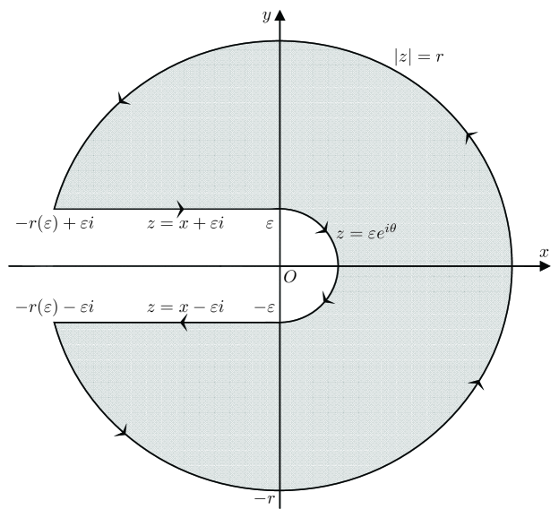
Figure 1. The contour $C(\varepsilon,r)$

By Cauchy integral formula, that is, Lemma 2.1, we have

$$\begin{split}h_{n}(z)&=\frac{1}{2\pi i}\oint_{C(\varepsilon,r)}\frac{h_{n}(w)}{w-z}\operatorname{d\mspace{-2.0mu}}w\\ &=\frac{1}{2\pi i}\biggl{[}\int_{\pi/2}^{-\pi/2}\frac{i\varepsilon e^{i\theta}h\bigl{(}\varepsilon e^{i\theta}\bigr{)}}{\varepsilon e^{i\theta}-z}\operatorname{d\mspace{-2.0mu}}\theta+\int_{\arg[-r(\varepsilon)-i\varepsilon]}^{\arg[-r(\varepsilon)+i\varepsilon]}\frac{ire^{i\theta}h\bigl{(}re^{i\theta}\bigr{)}}{re^{i\theta}-z}\operatorname{d\mspace{-2.0mu}}\theta\\ &\quad+\int_{-r(\varepsilon)}^{0}\frac{h_{n}(x+i\varepsilon)}{x+i\varepsilon-z}\operatorname{d\mspace{-2.0mu}}x+\int_{0}^{-r(\varepsilon)}\frac{h_{n}(x-i\varepsilon)}{x-i\varepsilon-z}\operatorname{d\mspace{-2.0mu}}x\biggr{]}.\end{split}$$ (3.3)

By the limit in (3.2), it follows that

$$\lim_{\varepsilon\to 0^{+}}\int_{\pi/2}^{-\pi/2}\frac{i\varepsilon e^{i\theta}h_{n}\bigl{(}\varepsilon e^{i\theta}\bigr{)}}{\varepsilon e^{i\theta}-z}\operatorname{d\mspace{-2.0mu}}\theta=0.$$ (3.4)

By virtue of the limit (2.3) in Lemma 2.2, we deduce that

$$\begin{split}\lim_{\begin{subarray}{c}\varepsilon\to 0^{+}\\ r\to\infty\end{subarray}}\int_{\arg[-r(\varepsilon)-i\varepsilon]}^{\arg[-r(\varepsilon)+i\varepsilon]}\frac{ire^{i\theta}h_{n}\bigl{(}re^{i\theta}\bigr{)}}{re^{i\theta}-z}\operatorname{d\mspace{-2.0mu}}\theta&=\lim_{r\to\infty}\int_{-\pi}^{\pi}\frac{ire^{i\theta}h_{n}\bigl{(}re^{i\theta}\bigr{)}}{re^{i\theta}-z}\operatorname{d\mspace{-2.0mu}}\theta\\ &=2A_{n}\bigl{(}[a]-a_{[1]}\bigr{)}\pi i,\end{split}$$ (3.5)

where $[a]-a_{[1]}=\bigl{(}0,a_{[2]}-a_{[1]},\dotsc,a_{[n]}-a_{[1]}\bigr{)}$. Utilizing the second formula in (3.2) and the limit (2.5) in Lemma 2.3 results in

$$\quad\int_{-r(\varepsilon)}^{0}\frac{h_{n}(x+i\varepsilon)}{x+i\varepsilon-z}\operatorname{d\mspace{-2.0mu}}x+\int_{0}^{-r(\varepsilon)}\frac{h_{n}(x-i\varepsilon)}{x-i\varepsilon-z}\operatorname{d\mspace{-2.0mu}}x$$

$$=\int_{-r(\varepsilon)}^{0}\biggl{[}\frac{h_{n}(x+i\varepsilon)}{x+i\varepsilon-z}-\frac{h_{n}(x-i\varepsilon)}{x-i\varepsilon-z}\biggr{]}\operatorname{d\mspace{-2.0mu}}x$$

$$=\int_{-r(\varepsilon)}^{0}\frac{(x-i\varepsilon-z)h_{n}(x+i\varepsilon)-(x+i\varepsilon-z)h_{n}(x-i\varepsilon)}{(x+i\varepsilon-z)(x-i\varepsilon-z)}\operatorname{d\mspace{-2.0mu}}x$$

$$=\int_{-r(\varepsilon)}^{0}\frac{(x-z)[h_{n}(x+i\varepsilon)-h_{n}(x-i\varepsilon)]-i\varepsilon[h_{n}(x-i\varepsilon)+h_{n}(x+i\varepsilon)]}{(x+i\varepsilon-z)(x-i\varepsilon-z)}\operatorname{d\mspace{-2.0mu}}x$$

$$=2i\int_{-r(\varepsilon)}^{0}\frac{(x-z)\Im h_{n}(x+i\varepsilon)-\varepsilon\Re h_{n}(x+i\varepsilon)}{(x+i\varepsilon-z)(x-i\varepsilon-z)}\operatorname{d\mspace{-2.0mu}}x$$

$$\to 2i\int_{-r}^{0}\frac{\lim_{\varepsilon\to 0^{+}}\Im h_{n}(x+i\varepsilon)}{x-z}\operatorname{d\mspace{-2.0mu}}x$$

$$=-2i\int^{r}_{0}\frac{\lim_{\varepsilon\to 0^{+}}\Im h_{n}(-t+i\varepsilon)}{t+z}\operatorname{d\mspace{-2.0mu}}t$$

$$\to-2i\int^{\infty}_{0}\frac{\lim_{\varepsilon\to 0^{+}}\Im h_{n}(-t+i\varepsilon)}{t+z}\operatorname{d\mspace{-2.0mu}}t$$

$$=-2i\sum_{\ell=1}^{n-1}\sin\frac{\ell\pi}{n}\int_{a_{[\ell]}-a_{[1]}}^{a_{[\ell+1]}-a_{[1]}}\Biggl{[}\prod_{k=1}^{n}\bigl{|}a_{[k]}-a_{[1]}-t\bigr{|}\Biggr{]}^{1/n}\frac{\operatorname{d\mspace{-2.0mu}}t}{t+z}$$ (3.6)

as $\varepsilon\to 0^{+}$ and $r\to\infty$. Substituting equations (3.4), (3.5), and (3.6) into (3.3) and simplifying generate

$$h_{n}(z)=A_{n}\bigl{(}[a]-a_{[1]}\bigr{)}-\frac{1}{\pi}\sum_{\ell=1}^{n-1}\sin\frac{\ell\pi}{n}\int_{a_{[\ell]}-a_{[1]}}^{a_{[\ell+1]}-a_{[1]}}\Biggl{[}\prod_{k=1}^{n}\bigl{|}a_{[k]}-a_{[1]}-t\bigr{|}\Biggr{]}^{1/n}\frac{\operatorname{d\mspace{-2.0mu}}t}{t+z}.$$ (3.7)

From (2.2) and (2.4), it is easy to obtain that

$$f_{a,n}(z)=h_{n}\bigl{(}z+a_{[1]}\bigr{)}+a_{[1]}.$$

Combining this with (3.7) and changing the variables of integrals, it is immediate to deduce that

$$f_{a,n}(z) =A_{n}\bigl{(}[a]-a_{[1]}\bigr{)}+a_{[1]}$$

$$\quad-\frac{1}{\pi}\sum_{\ell=1}^{n-1}\sin\frac{\ell\pi}{n}\int_{a_{[\ell]}-a_{[1]}}^{a_{[\ell+1]}-a_{[1]}}\Biggl{[}\prod_{k=1}^{n}\bigl{|}a_{[k]}-a_{[1]}-t\bigr{|}\Biggr{]}^{1/n}\frac{\operatorname{d\mspace{-2.0mu}}t}{t+z+a_{[1]}}$$

$$=A_{n}([a])-\frac{1}{\pi}\sum_{\ell=1}^{n-1}\sin\frac{\ell\pi}{n}\int_{a_{[\ell]}}^{a_{[\ell+1]}}\Biggl{[}\prod_{k=1}^{n}|a_{[k]}-t|\Biggr{]}^{1/n}\frac{\operatorname{d\mspace{-2.0mu}}t}{t+z},$$

from which and the facts that

$$A_{n}([a])=A_{n}(a)\quad\text{and}\quad\prod_{k=1}^{n}|a_{[k]}-t|=\prod_{k=1}^{n}|a_{k}-t|,$$

the integral representation (3.1) follows.

Differentiating with respect to $z$ on both sides of (3.1) yields

$$G_{n}^{\prime}(a+z)=1+\frac{1}{\pi}\sum_{\ell=1}^{n-1}\sin\frac{\ell\pi}{n}\int_{a_{[\ell]}}^{a_{[\ell+1]}}\Biggl{[}\prod_{k=1}^{n}|a_{k}-t|\Biggr{]}^{1/n}\frac{\operatorname{d\mspace{-2.0mu}}t}{(t+z)^{2}},$$

which implies that $G_{n}^{\prime}(a+t)$ is completely monotonic, and so the geometric mean $G_{n}(a+t)$ is a Bernstein function. Theorem 3.1 is proved. ∎

4. A new proof of the AG inequality

As an application of the integral representation (3.1) in Theorem 3.1, we can easily deduce the AG inequality (1.20) as follows.

Taking $z=0$ in the integral representation (3.1) yields

$$G_{n}(a)=A_{n}(a)-\frac{1}{\pi}\sum_{\ell=1}^{n-1}\sin\frac{\ell\pi}{n}\int_{a_{[\ell]}}^{a_{[\ell+1]}}\Biggl{[}\prod_{k=1}^{n}|a_{k}-t|\Biggr{]}^{1/n}\frac{\operatorname{d\mspace{-2.0mu}}t}{t}\leq A_{n}(a),$$ (4.1)

from which the inequality (1.20) follows.

From (4.1), it is also immediate that the equality in (1.20) is valid if and only if $a_{[1]}=a_{[2]}=\dotsm=a_{[n]}$, that is, $a_{1}=a_{2}=\dotsm=a_{n}$. The proof of the AG inequality (1.20) is complete.

References

- [1] R. D. Atanassov and U. V. Tsoukrovski, Some properties of a class of logarithmically completely monotonic functions, C. R. Acad. Bulgare Sci. 41 (1988), no. 2, 21–23.
- [2] E. F. Beckenbach and R. Bellman, Inequalities, Springer, Berlin, 1983.
- [3] C. Berg, Integral representation of some functions related to the gamma function, Mediterr. J. Math. 1 (2004), no. 4, 433–439; Available online at http://dx.doi.org/10.1007/s00009-004-0022-6.
- [4] P. S. Bullen, Handbook of Means and Their Inequalities, Mathematics and its Applications (Dordrecht) 560, Kluwer Academic Publishers, Dordrecht, 2003.
- [5] C.-P. Chen, F. Qi, and H. M. Srivastava, Some properties of functions related to the gamma and psi functions, Integral Transforms Spec. Funct. 21 (2010), no. 2, 153–164; Available online at http://dx.doi.org/10.1080/10652460903064216.
- [6] T. W. Gamelin, Complex Analysis, Undergraduate Texts in Mathematics, Springer, New York-Berlin-Heidelberg, 2001.
- [7] B.-N. Guo and F. Qi, A completely monotonic function involving the tri-gamma function and with degree one, Appl. Math. Comput. 218 (2012), no. 19, 9890–9897; Available online at http://dx.doi.org/10.1016/j.amc.2012.03.075.
- [8] B.-N. Guo and F. Qi, A property of logarithmically absolutely monotonic functions and the logarithmically complete monotonicity of a power-exponential function, Politehn. Univ. Bucharest Sci. Bull. Ser. A Appl. Math. Phys. 72 (2010), no. 2, 21–30.
- [9] B.-N. Guo and F. Qi, A simple proof of logarithmic convexity of extended mean values, Numer. Algorithms 52 (2009), no. 1, 89–92; Available online at http://dx.doi.org/10.1007/s11075-008-9259-7.
- [10] B.-N. Guo and F. Qi, The function : Logarithmic convexity and applications to extended mean values, Filomat 25 (2011), no. 4, 63–73; Available online at http://dx.doi.org/10.2298/FIL1104063G.
- [11] B.-N. Guo and F. Qi, The function : Ratio’s properties, Available online at http://arxiv.org/abs/0904.1115.
- [12] G. H. Hardy, J. E. Littlewood, and G. Pólya, Inequalities, 2nd ed., Cambridge University Press, Cambridge, 1952.
- [13] J.-C. Kuang, Chángyòng Bùděngshì (Applied Inequalities), 3rd ed., Shāndōng Kēxué Jìshù Chūbǎn Shè (Shandong Science and Technology Press), Ji’nan City, Shandong Province, China, 2004. (Chinese)
- [14] D. S. Mitrinović, Analytic Inequalities, Springer, New York-Heidelberg-Berlin, 1970.
- [15] D. S. Mitrinović, J. E. Pečarić, and A. M. Fink, Classical and New Inequalities in Analysis, Kluwer Academic Publishers, 1993.
- [16] D. S. Mitrinović and P. M. Vasić, Sredine, Matematička Biblioteka 40, Beograd, 1969.
- [17] F. Qi, A new lower bound in the second Kershaw’s double inequality, J. Comput. Appl. Math. 214 (2008), no. 2, 610–616; Availbale online at http://dx.doi.org/10.1016/j.cam.2007.03.016.
- [18] F. Qi and C.-P. Chen, A complete monotonicity property of the gamma function, J. Math. Anal. Appl. 296 (2004), no. 2, 603–607; Available online at http://dx.doi.org/10.1016/j.jmaa.2004.04.026.
- [19] F. Qi and S.-X. Chen, Complete monotonicity of the logarithmic mean, Math. Inequal. Appl. 10 (2007), no. 4, 799–804; Available online at http://dx.doi.org/10.7153/mia-10-73.
- [20] F. Qi and B.-N. Guo, Complete monotonicities of functions involving the gamma and digamma functions, RGMIA Res. Rep. Coll. 7 (2004), no. 1, Art. 8, 63–72; Available online at http://rgmia.org/v7n1.php.
- [21] F. Qi, S. Guo, and S.-X. Chen, A new upper bound in the second Kershaw’s double inequality and its generalizations, J. Comput. Appl. Math. 220 (2008), no. 1-2, 111–118; Available online at http://dx.doi.org/10.1016/j.cam.2007.07.037.
- [22] F. Qi, C.-F. Wei, and B.-N. Guo, Complete monotonicity of a function involving the ratio of gamma functions and applications, Banach J. Math. Anal. 6 (2012), no. 1, 35–44.
- [23] F. Qi, X.-J. Zhang, and W.-H. Li, Some Bernstein functions and integral representations concerning harmonic and geometric means, available online at http://arxiv.org/abs/1301.6430.
- [24] R. L. Schilling, R. Song, and Z. Vondraček, Bernstein Functions, de Gruyter Studies in Mathematics 37, De Gruyter, Berlin, Germany, 2010.
- [25] K. B. Stolarsky, Generalizations of the logarithmic mean, Math. Mag. 48 (1975), 87–92.
- [26] D. V. Widder, The Laplace Transform, Princeton University Press, Princeton, 1946.