MPP-2013-13

SISSA 04/2013/FISI

Spontaneous CP violation in $\boldsymbol{A_{4}\times SU(5)}$ with Constrained Sequential Dominance 2

Stefan Antusch^⋆ , Stephen F. King^† , Martin Spinrath^‡ ,

^⋆ Department of Physics, University of Basel,

Klingelbergstr. 82, CH-4056 Basel, Switzerland

^⋆ Max-Planck-Institut für Physik (Werner-Heisenberg-Institut),

Föhringer Ring 6, D-80805 München, Germany

^† School of Physics and Astronomy, University of Southampton,

SO17 1BJ Southampton, United Kingdom

^‡ SISSA/ISAS and INFN,

Via Bonomea 265, I-34136 Trieste, Italy

We revisit a two right-handed neutrino model with two texture zeros, namely an indirect model based on $A_{4}$ with the recently proposed new type of constrained sequential dominance (CSD2), involving vacuum alignments along the $(0,1,-1)^{T}$ and $(1,0,2)^{T}$ directions in flavour space, which are proportional to the neutrino Dirac mass matrix columns. In this paper we construct a renormalizable and unified indirect $A_{4}\times SU(5)$ model along these lines and show that, with spontaneous CP violation and a suitable vacuum alignment of the phases, the charged lepton corrections lead to a reactor angle in good agreement with results from Daya Bay and RENO. The model predicts a right-angled unitarity triangle in the quark sector and a Dirac CP violating oscillation phase in the lepton sector of $\delta\approx 130^{\circ}$, while providing a good fit to all quark and lepton masses and mixing angles.

1 Introduction

The lepton mixing angles have the distinctive feature that the atmospheric angle $\theta_{23}$ and the solar angle $\theta_{12}$, are both rather large [1]. Direct evidence for the reactor angle $\theta_{13}$ was first provided by T2K, MINOS and Double Chooz [4, 2, 3]. Subsequently Daya Bay [5], RENO [6], and Double Chooz [7] Collaborations have measured $\sin^{2}(2\theta_{13})$:

$$\begin{array}[]{cc}\text{Daya Bay: }&\sin^{2}(2\theta_{13})=0.089\pm 0.011\text{(stat.)}\pm 0.005\text{(syst.)}\ ,\\ \text{RENO: }&\sin^{2}(2\theta_{13})=0.113\pm 0.013\text{(stat.)}\pm 0.019\text{(syst.)\ ,}\\ \text{Double Chooz: }&\sin^{2}(2\theta_{13})=0.109\pm 0.030\text{(stat.)}\pm 0.025\text{(syst.)}\ .\\ \end{array}$$ (1.4)

This rules out the hypothesis of exact tri-bimaximal (TB) mixing [8], and many alternative proposals have recently been put forward [9], although there are relatively few examples which also include unification [10, 11, 12, 13]. For example, an attractive scheme based on trimaximal (TM) mixing remains viable [14], sometimes referred to as TM₂ mixing since it maintains the second column of the TB mixing matrix and hence preserves the solar mixing angle prediction $\sin\theta_{12}\approx 1/\sqrt{3}$. However there is another variation of TM mixing which also preserves this good solar mixing angle prediction by maintaining the first column of the TB matrix, namely TM₁ mixing [15].

Although there were models of TM₂ mixing which can account for the smallness of the reactor angle [16], the first model in the literature for TM₁ mixing, which also fixed the value of the reactor angle, was proposed in [17]. The model discussed in [17] was actually representative of a general strategy for obtaining TM₁ mixing using sequential dominance (SD) [18] and vacuum alignment. The strategy of combining SD with vacuum alignment is familiar from the constrained sequential dominance (CSD) approach to TB mixing [19] where a neutrino mass hierarchy is assumed and the dominant and subdominant flavons responsible for the atmospheric and solar neutrino masses are aligned in the directions of the third and second columns of the TB mixing matrix, namely $\langle\phi_{1}^{\nu}\rangle\propto(0,1,-1)^{T}$ and $\langle\phi_{2}^{\nu}\rangle\propto(1,1,1)^{T}$. The new idea was to maintain the usual vacuum alignment for the dominant flavon, $\langle\phi_{1}^{\nu}\rangle\propto(0,1,-1)^{T}$ as in CSD, but to replace the effect of the subdominant flavon vacuum alignment by a different one, namely either $\langle\phi_{120}\rangle\propto(1,2,0)^{T}$ or $\langle\phi_{102}\rangle\propto(1,0,2)^{T}$, where such alignments may be naturally achieved from the standard ones using orthogonality arguments.

We referred to this new approach as CSD2 and showed that it leads to TM₁ mixing and a reactor angle which, at leading order, is predicted to be proportional to the ratio of the solar to the atmospheric neutrino masses, $\theta_{13}=\frac{\sqrt{2}}{3}\,\frac{m^{\nu}_{2}}{m^{\nu}_{3}}$. The model was proposed before the results from Daya Bay and RENO, and the prediction turned out to be rather too small compared to the results in Eq. (1.4). More generally it has been shown that any type I seesaw model with two right-handed neutrinos and two texture zeros in the neutrino Yukawa matrix (as in Occam’s razor) is not compatible with the experimental data for the case of a normal neutrino mass hierarchy [21]. However this conclusion ignores the effect of charged lepton corrections, and so an “Occam’s razor” model which includes such corrections may become viable.

In the present paper we construct a fully renormalisable unified $A_{4}\times SU(5)$ model in which the neutrino sector satisfies the CSD2 conditions, and show that, with spontaneous CP violation and a suitable vacuum alignment of the phases, the charged lepton corrections can correct the reactor angle, bringing it into agreement with results from Daya Bay and RENO. We shall use here similar techniques as in [22], where spontaneous CP violation with flavon phases determined by the vacuum alignment was discussed for the first time, in order to ensure that the charged lepton mixing angle correction (typically about $\sim 3^{\circ}$) adds constructively to the $\theta_{13}^{\nu}$ angle from the neutrino sector (typically about $\sim 5^{\circ}-6^{\circ}$) leading to $\theta_{13}\sim 8^{\circ}-9^{\circ}$, within the range of the measured value from Daya Bay and RENO. In fact the present model is more ambitious, since it describes all quark and lepton masses and mixing angles, including predictions for all the CP violating phases.

We demonstrate the viability of the model by performing a global fit to the charged lepton masses and the quark masses and mixing parameters. For the neutrino mixing angles we make a parameter scan and find very good agreement with the experimental data. We emphasise that the present $A_{4}\times SU(5)$ model represents one of the first unified “indirect” family symmetry models in the literature that has been constructed to date that is consistent with all experimental data on quark and lepton mass and mixing parameters where “indirect” simply means that the family symmetry is completely broken by the vacuum alignment. For a review see [23].

We emphasise that the idea of spontaneous CP violation has a long history [24]. However, in explicit flavour models using this idea only the positions of the phases in the mass matrices was predicted, but not the phases of the flavon fields themselves (see e.g. [25]). Spontaneous CP violation with calculable flavon phases from vacuum alignment was first discussed in [22] and demonstrated in example models based on $A_{4}$ and $S_{4}$. In this paper we shall use a similar approach where the $A_{4}$ model is formulated in the real $SO(3)$ basis (see e.g. [26]) and where we only consider the real representations $\mathbf{1}$ and $\mathbf{3}$. In such a framework, one can either use a “simple” CP symmetry under which the components of the scalar fields transform trivially as $\phi_{i}\rightarrow\phi_{i}^{*}$, or a “generalised” CP symmetry which intertwines CP with $A_{4}$ (see e.g. [27] and references therein). In the latter case, in our basis, the triplet fields would transform as $\phi_{i}\rightarrow U_{3}\phi_{i}^{*}$, where $U_{3}$ interchanges the second and third component. When complex $\mathbf{1}^{\prime}$ and $\mathbf{1}^{\prime\prime}$ representations are used in a model, the $U_{3}$ transformation then takes care of the fact that under CP the two complex singlets are interchanged with each other. However, as already mentioned above, in our model this will make no difference. CP symmetry leads to real coupling constants in a suitable field basis (after “unphysical” phases have been absorbed by field redefinitions). CP is subsequently spontaneously broken by the flavon vacuum alignment, which is controlled by additional Abelian symmetries $\mathbb{Z}_{3}$ and $\mathbb{Z}_{4}$, resulting in calculable complex flavon phases as in [22].

The layout of the rest of the paper is as follows: in the next section we discuss the general strategy we will adopt in our model. After a brief review of CSD2 we discuss charged lepton sector corrections to TM₁ mixing before we describe the method which we use to fix the flavon vevs. In section 3 we describe our model, the field content and symmetries and the resulting Yukawa and mass matrices. The justification for the chosen vacuum alignment including phases is given in section 4. In the subsequent sections we comment on the Higgs mass and then we give the numerical results from our global fit and scans. In section 7 we summarize and conclude and in the appendix we define our notations and conventions and give the messenger sector of our model.

2 The strategy

Let us now describe our general idea in somewhat more detail, before we present an explicit GUT model example in the next section. As outlined in the introduction, we are combining three ingredients which finally result in a highly predictive unified flavour model. These ingredients are:

• CSD2 for the neutrino mixing angles $\theta_{ij}^{\nu}$,

• charged lepton mixing contributions as they are typical in GUTs,

• spontaneous CP violation with aligned phases.

We now briefly describe these three concepts and the resulting new class of models.

CSD2 in the neutrino sector

In models with CSD2 [17], the neutrino mass matrix is dominated by two right-handed neutrinos with mass matrix $M_{R}={\rm diag}(M_{A},M_{B})$ and couplings to the lepton doublets $A=(0,a,-a)^{T}$ and $B=(b,0,2b)^{T}$ such that the neutrino Yukawa matrix takes the form $Y_{\nu}=(A,B)$, in left-right convention. A summary of the used conventions is given in the Appendix.

After the seesaw mechanism is implemented, CSD2 leads to the following light effective neutrino Majorana mass matrix:

$$M_{\nu}=m_{a}\begin{pmatrix}0&0&0\\ 0&1&-1\\ 0&-1&1\end{pmatrix}+m_{b}\begin{pmatrix}1&0&2\\ 0&0&0\\ 2&0&4\end{pmatrix}=m_{a}\begin{pmatrix}\epsilon\,\text{e}^{\operatorname{\text{i}}\alpha}&0&2\epsilon\,\text{e}^{\operatorname{\text{i}}\alpha}\\ 0&1&-1\\ 2\epsilon\,\text{e}^{\operatorname{\text{i}}\alpha}&-1&1+4\epsilon\,\text{e}^{\operatorname{\text{i}}\alpha}\end{pmatrix},$$ (2.1)

where $m_{a}=\frac{v_{u}^{2}a^{2}}{M_{A}}$, $m_{b}=\frac{v_{u}^{2}b^{2}}{M_{B}}$, and where $\alpha$ is the relative phase difference between $m_{a}$ and $m_{b}$. We define $\epsilon=|m_{b}|/|m_{a}|$, and assume $\epsilon\ll 1$ leading to a normal mass hierarchy in accordance with SD. As discussed in Appendix A we use here different conventions than in the original CSD2 paper [17] which are more convenient in the context of $SU(5)$ GUTs.

Only three parameters, e.g. $m_{a}$, $\epsilon$ and $\alpha$, govern the neutrino masses and mixing parameters. For the mixing parameters, the predicted values are, to leading order in $\epsilon$ (from [17] with adapted conventions):

$$s_{23}^{\nu} \approx\frac{1}{\sqrt{2}}-\frac{\epsilon}{\sqrt{2}}\cos\alpha\;, \delta_{13}^{\nu} \approx\pi-\alpha+\epsilon\frac{5}{2}\sin\alpha\;,$$ (2.2)

$$s_{13}^{\nu} \approx\frac{\epsilon}{\sqrt{2}}\;, \alpha_{2} \approx-\alpha+2\epsilon\sin\alpha\;,$$ (2.3)

$$s_{12}^{\nu} \approx\frac{1}{\sqrt{3}}\;.$$ (2.4)

The mixing scheme resulting from CSD2 can be identified as trimaximal mixing of type 1 (i.e. TM₁ [15]) but with a predicted value of the neutrino 1-3 mixing, $\theta^{\nu}_{13}=\frac{\sqrt{2}}{3}\frac{m^{\nu}_{2}}{m^{\nu}_{3}}\sim 5^{\circ}-6^{\circ}$. With neutrino mass $m^{\nu}_{1}=0$, only one Majorana CP phase is physical. Without charged lepton corrections, $\delta_{13}^{\nu}$ would be identical with the leptonic Dirac CP phase $\delta$. Let us also note that CSD2 predicts a deviation of $\theta_{23}^{\nu}$ from $45^{\circ}$, depending on the phase $\alpha$.

Charged lepton mixing contribution in GUTs

In GUT models the charged lepton Yukawa matrix is generically non-diagonal in the flavour basis, due to the close link between the charged lepton and the down-type quark Yukawa matrices, which typically provides the main origin of the flavour mixing in the quark sector. With the Cabibbo angle $\theta_{C}$ being the largest mixing in the quark sector, the mixing in $Y_{e}$ is often dominated by a 1-2 mixing $\theta^{e}_{12}$ as well, such that the relevant part of (the hierarchical matrix) $Y_{e}$ can be written as

$$Y_{e}\approx\begin{pmatrix}0&c\,\text{e}^{\operatorname{\text{i}}\beta}&0\\ *&d&0\\ 0&*&*\end{pmatrix}\;,$$ (2.5)

where $c$, $d$, and $\beta$ are real and where the entries marked by a ’$*$’ are not relevant for our discussion here. With $c\ll d$ one can read off to leading order the values for the complex 1-2 mixing angle (for more details see also Appendix A) that are

$$\theta_{12}^{e}\approx\left|\frac{c}{d}\right|\text{ and }\delta^{e}_{12}=\begin{cases}-\beta&\text{for }c/d>0\\ -\beta+\pi&\text{for }c/d<0\end{cases}\;.$$ (2.6)

Since we will have $c/d<0$ in our example GUT model in the next section, let us consider this case also in the following discussion.

In explicit GUT models, $\theta^{e}_{12}$ is typically related to the Cabibbo angle by group theoretical Clebsch factors from GUT breaking, as has been discussed recently, e.g. in [10, 11]. In many GUT models, in particular in those where the muon and the strange quark mass at the GUT scale is predicted by such a Clebsch factor as $m_{\mu}/m_{s}=3$ [28], but also if the Yukawa matrices $Y_{e}$ (and $Y_{d}$) are (nearly) symmetric with a zero in the (0,0)-element [10], $\theta_{12}^{e}$ is predicted as

$$\theta_{12}^{e}\approx\frac{\theta_{C}}{3}\;.$$ (2.7)

In the example GUT model in the next section we will see explicitly how such a prediction arises in an $SU(5)$ GUT.

The leptonic mixing parameters, defined via $U_{\text{PMNS}}=U_{e}U_{\nu}^{\dagger}$, are a combination of the mixing from the neutrino and the charged lepton sectors. Making use of the fact that, to leading order, $\theta_{23}^{e}=\theta_{13}^{e}=\delta_{12}^{\nu}=\delta_{23}^{\nu}=0$, and using the CSD2 expressions from above for the neutrino sector, and general formulae for the charged lepton mixing contributions of [29, 19, 30]

$$s_{23}\text{e}^{-\operatorname{\text{i}}\delta_{23}} =s_{23}^{\nu}\text{e}^{-\operatorname{\text{i}}\delta_{23}^{\nu}}-\theta_{23}^{e}c_{23}^{\nu}\text{e}^{-\operatorname{\text{i}}\delta_{23}^{e}}\;,$$ (2.8)

$$s_{13}\text{e}^{-\operatorname{\text{i}}\delta_{13}} =\theta_{13}^{\nu}\text{e}^{-\operatorname{\text{i}}\delta_{13}^{\nu}}-\theta_{12}^{e}s_{23}^{\nu}\text{e}^{-\operatorname{\text{i}}(\delta_{23}^{\nu}+\delta_{12}^{e})}\;,$$ (2.9)

$$s_{12}\text{e}^{-\operatorname{\text{i}}\delta_{12}} =s_{12}^{\nu}\text{e}^{-\operatorname{\text{i}}\delta_{12}^{\nu}}-\theta_{12}^{e}c_{23}^{\nu}c_{12}^{\nu}\text{e}^{-\operatorname{\text{i}}\delta_{12}^{e}}\;,$$ (2.10)

we obtain (up to $\mathcal{O}(\epsilon)$)

$$\theta_{23} \approx 45^{\circ}-\epsilon\cos\alpha\;,$$ (2.11)

$$\theta_{13} \approx\frac{\epsilon}{\sqrt{2}}-\cos(\beta-\alpha)\,\frac{\theta_{12}^{e}}{\sqrt{2}}\;,$$ (2.12)

$$\theta_{12} \approx 35.3^{\circ}+\cos\beta\,\frac{\theta_{12}^{e}}{\sqrt{2}}\;,$$ (2.13)

where $\epsilon\approx\frac{2}{3}\frac{m^{\nu}_{2}}{m^{\nu}_{3}}\approx 8.4^{\circ}$. When the phases $\alpha$ and $\beta$ are fixed by the vacuum alignment, and when also $\theta_{12}^{e}$ is predicted from the GUT structure, as both will be the case in our model, all three mixing angles and also the CP phases $\delta$ and $\alpha_{2}$, are predicted. Thus, the resulting models of this type can be highly predictive.

We would like to note here already that in the explicit GUT model in the next section, we will construct a vacuum alignment such that $\alpha=\pi/3$, leading to

$$\theta_{23}\approx 45^{\circ}-\frac{\epsilon}{2}\approx 41^{\circ}\>,$$ (2.14)

close to the best fit value for the normal hierarchy case from global fits to the neutrino data [31]. The alignment of $\beta$ will satisfy $\beta=\alpha+\pi$, such that the neutrino and charged lepton contributions to $\theta_{13}$ simply add up, leading to (with $\theta_{12}^{e}=\theta_{C}/3$)

$$\theta_{13}\approx\frac{\epsilon}{\sqrt{2}}+\frac{\theta_{C}}{3\sqrt{2}}\approx 8^{\circ}-9^{\circ}\;,$$ (2.15)

in agreement with the recent measurements. With these values of $\alpha$ and $\beta$, it also turns out that $\theta_{12}$ is predicted somewhat smaller than $35^{\circ}$, namely

$$\theta_{12}\sim 33^{\circ}\;.$$ (2.16)

This value of $\theta_{12}$ could be distinguished from the tribimaximal value by a future reactor experiment with $\sim 60$ km baseline [32].

Spontaneous CP violation with aligned phases

Finally, the third ingredient is spontaneous CP violation with aligned phases of the flavon vevs, using the method proposed in [22]. To give a brief summary of this method, let us note that phase alignment can very simply be achieved using discrete symmetries when the flavon vevs effectively depend on one parameter, i.e. when the direction of the vevs is given by the form of the potential. This remains true even in the presence of “generalised” CP transformations as long as these CP transformations fix the phases of the involved coupling constants. Working example models with $A_{4}$ and $S_{4}$ family symmetry can be found in [22]. Note that $S_{4}$ is in agreement only with “simple” CP, while the “generalised” CP transformation for $A_{4}$ interchanges the complex singlet representations [27]. In both cases all the coupling constants are forced to be real in a suitable field basis.

To illustrate the phase alignment, let us consider a case with a flavon field $\xi$ which is a singlet under the family symmetry and singly charged under a $\mathbb{Z}_{n}$ shaping symmetry (with $n\geq 2$). Then typical terms in the flavon superpotential, which “drive” the flavon vev non-zero, have the form

$$P\left(\frac{\xi^{n}}{\Lambda^{n-2}}\mp M^{2}\right).$$ (2.17)

The field $P$ is the so-called “driving superfield”, meaning that the $F$-term $|F_{P}|^{2}$ generates the potential for $\xi$ which enforces a non-zero vev. $\Lambda$ is the (real and positive) suppression scale of the effective operator, and $M$ here is simply a (real) mass scale. From the potential for $\xi$,

$$|F_{P}|^{2}=\left|\frac{\xi^{n}}{\Lambda^{n-2}}\mp M^{2}\right|^{2},$$ (2.18)

the vev of $\xi$ has to satisfy

$$\xi^{n}=\pm\,\Lambda^{n-2}M^{2}\;.$$ (2.19)

Since the right side of the equation is real, we obtain that

$$\arg(\langle\xi\rangle)=\left\{\begin{array}[]{ll}\frac{2\pi}{n}q\;,\quad q=1,\dots,n&\mbox{\vphantom{$\frac{f}{f}$} for ``$-$'' in Eq.~{}(\ref{eq:flavonpotentialZn}),}\\ \frac{2\pi}{n}q+\frac{\pi}{n}\;,\quad q=1,\dots,n&\mbox{\vphantom{$\frac{f}{f}$} for ``$+$'' in Eq.~{}(\ref{eq:flavonpotentialZn}).}\end{array}\right.$$ (2.20)

For example, with a $\mathbb{Z}_{3}$ shaping symmetry and a “$+$” in Eq. (2.17), only multiples of $\pi/3$ are allowed for $\arg(\langle\xi\rangle)$. We will use this method for the relevant flavons to constrain their phases. In the ground state, one of the vacua (with a fixed phase) is selected, which finally determines also the two phases $\alpha$ and $\beta$ relevant for the predictions in the lepton sector.

Furthermore, we note that we will also use the phase alignment to generate the CP violation in the quark sector, predicting a right-angled unitarity triangle, which is in excellent agreement with the present data (making use of the quark phase sum rule from [33]).

We now turn to an explicit GUT model, where the above described strategy is applied.

3 The model

In the following we will construct an $A_{4}\times SU(5)$ model with CSD2 [17] in the neutrino sector. The model follows the strategy described in the previous section, such that the charged lepton mixing contribution to $\theta_{13}$ adds up constructively with the 1-3 mixing in the neutrino sector to $\theta_{13}\sim 8^{\circ}-9^{\circ}$, with the phases fixed by the “discrete vacuum alignment” mechanism [22].

	$T_{1}$	$T_{2}$	$T_{3}$	$F$	$N_{1}$	$N_{2}$	$H_{5}$	$\bar{H}_{5}$	$H_{45}$	$\bar{H}_{45}$	$H_{24}$	$S$
$SU(5)$	$\mathbf{10}$	$\mathbf{10}$	$\mathbf{10}$	$\mathbf{\bar{5}}$	$\mathbf{1}$	$\mathbf{1}$	$\mathbf{5}$	$\mathbf{\bar{5}}$	$\mathbf{45}$	$\mathbf{\overline{45}}$	$\mathbf{24}$	$\mathbf{1}$
$A_{4}$	$\mathbf{1}$	$\mathbf{1}$	$\mathbf{1}$	$\mathbf{3}$	$\mathbf{1}$	$\mathbf{1}$	$\mathbf{1}$	$\mathbf{1}$	$\mathbf{1}$	$\mathbf{1}$	$\mathbf{1}$	$\mathbf{1}$
$U(1)_{R}$	1	1	1	1	1	1	0	0	0	0	0	2
$\mathbb{Z}_{4}$	3	3	3	0	0	2	2	0	0	2	1	2
$\mathbb{Z}_{4}$	3	3	3	0	2	2	2	0	2	0	1	2
$\mathbb{Z}_{3}$	1	2	0	0	1	2	0	0	0	0	2	0
$\mathbb{Z}_{3}$	1	1	0	0	2	0	0	0	1	2	2	0
$\mathbb{Z}_{3}$	0	2	2	1	0	2	2	0	1	1	2	1
$\mathbb{Z}_{3}$	0	0	0	2	0	0	0	0	1	2	1	0

Table 1: The matter and Higgs fields in our model and their quantum numbers.

	$SU(5)$	$A_{4}$	$U(1)_{R}$	$\mathbb{Z}_{4}$	$\mathbb{Z}_{4}$	$\mathbb{Z}_{3}$	$\mathbb{Z}_{3}$	$\mathbb{Z}_{3}$	$\mathbb{Z}_{3}$
$\phi_{102}$	$\mathbf{1}$	$\mathbf{3}$	0	0	0	1	0	1	1
$\phi_{23}$	$\mathbf{1}$	$\mathbf{3}$	0	2	0	2	1	0	1
$\phi_{1}$	$\mathbf{1}$	$\mathbf{3}$	0	1	3	1	0	0	1
$\phi_{2}$	$\mathbf{1}$	$\mathbf{3}$	0	0	3	0	0	0	0
$\phi_{3}$	$\mathbf{1}$	$\mathbf{3}$	0	1	1	0	0	0	1
$\phi_{111}$	$\mathbf{1}$	$\mathbf{3}$	0	3	3	0	0	0	0
$\phi_{211}$	$\mathbf{1}$	$\mathbf{3}$	0	0	0	2	1	1	0
$\xi_{u}$	$\mathbf{1}$	$\mathbf{1}$	0	0	0	0	2	1	0
$\xi_{1}$	$\mathbf{1}$	$\mathbf{1}$	0	0	0	1	2	0	0
$\xi_{2}$	$\mathbf{1}$	$\mathbf{1}$	0	0	0	2	0	2	0
$\theta_{2}$	$\mathbf{1}$	$\mathbf{1}$	0	0	1	0	0	0	0
$\theta_{102}$	$\mathbf{1}$	$\mathbf{1}$	0	0	0	1	0	0	2
$\rho_{111}$	$\mathbf{1}$	$\mathbf{1}$	0	3	3	0	0	0	0
$\tilde{\rho}_{111}$	$\mathbf{1}$	$\mathbf{1}$	0	3	3	0	0	0	0
$\rho_{23}$	$\mathbf{1}$	$\mathbf{1}$	0	0	0	2	1	0	1
$\rho_{102}$	$\mathbf{1}$	$\mathbf{1}$	0	0	0	1	0	1	1

Table 2: The flavon field content of our model.

The matter and the Higgs sector of the model is summarised in Table 1 while the required flavons are shown in Table 2. The superpotential after integrating out the heavy messenger fields, see Appendix B, and suppressing order one coefficients reads

$$\mathcal{W}_{N} =\xi_{1}N_{1}^{2}+\xi_{2}N_{2}^{2}\;,$$ (3.1)

$$\mathcal{W}_{\nu} =\frac{1}{\Lambda}(H_{5}F)(\phi_{23}N_{1})+\frac{1}{\Lambda}(H_{5}F)(\phi_{102}N_{2})\;,$$ (3.2)

$$\mathcal{W}_{d} =\frac{1}{\Lambda^{3}}\theta_{2}\bar{H}_{5}F(T_{1}\phi_{2})H_{24}+\frac{1}{\Lambda^{3}}\theta_{102}\bar{H}_{5}F(T_{2}\phi_{102})H_{24}+\frac{1}{\Lambda^{2}}F(T_{2}\phi_{23})\bar{H}_{45}H_{24}+\frac{1}{\Lambda}\bar{H}_{5}F(T_{3}\phi_{3})\;,$$ (3.3)

$$\mathcal{W}_{u} =\frac{1}{\Lambda^{2}}T_{1}^{2}H_{5}\xi_{u}\xi_{1}+\frac{1}{\Lambda^{2}}T_{1}T_{2}H_{5}\xi_{u}^{2}+\frac{1}{\Lambda^{2}}T_{2}^{2}H_{5}\xi_{1}^{2}+\frac{1}{\Lambda}T_{2}T_{3}H_{5}\xi_{1}+T_{3}^{2}H_{5}\;,$$ (3.4)

where $\Lambda$ denotes the messenger scale. The flavon potential, which gives rise to the vevs of the fields $\phi_{i}$, $\xi_{i}$ and $\theta_{i}$ will be discussed separately in the next section. Note that the flavons of type $\phi$ which enter the Yukawa couplings will be aligned with real vevs while the flavons of type $\theta$ and $\xi$ will generally acquire complex vevs with precisely determined phases. The above superpotential gives rise to the flavour structures in the neutrino sector, in the down-type quark and charged lepton sectors, and in the up-type quark sector.

Neutrino sector: From the flavon potential, to be discussed in the next section, the two triplet flavons entering the neutrino Yukawa sector are aligned along the directions

$$\langle\phi_{23}\rangle\sim\begin{pmatrix}0\\ 1\\ -1\end{pmatrix},\ \ \ \ \langle\phi_{102}\rangle\sim\begin{pmatrix}1\\ 0\\ 2\end{pmatrix}\;,\quad$$ (3.5)

where both alignments are real. Inserting the above vacuum alignments, the real vev $\langle\xi_{1}\rangle$ and the vev $\langle\xi_{2}\rangle$ with a phase of $-\pi/3$ into the superpotential leads to a Dirac Yukawa matrix and a right-handed heavy Majorana mass matrix of the form:

$$Y_{\nu}=\begin{pmatrix}0&b\\ a&0\\ -a&2b\end{pmatrix}\text{ and }\;\;M_{R}=\begin{pmatrix}M_{A}&0\\ 0&M_{B}\end{pmatrix}.$$ (3.6)

where $M_{A}$, $a$ and $b$ are real and $M_{B}$ has a complex phase of $-\pi/3$. The (type-I) seesaw formula leads to a simple effective light neutrino mass matrix of the form given in eq. (2.1) where the relative phase difference $\alpha$ between $m_{a}$ and $m_{b}$ is now fixed to be $\pi/3$. This form of $M_{\nu}$ gives $\theta^{\nu}_{13}\sim 5^{\circ}-6^{\circ}$ for the 1-3 mixing in the neutrino sector, which will finally add up with the charged lepton mixing contribution.

Down-type quark and charged lepton sector: Turning to the down quark and charged lepton sector, two further triplet flavons enter:

$$\langle\phi_{2}\rangle \sim\begin{pmatrix}0\\ 1\\ 0\end{pmatrix}\;,\quad\langle\phi_{3}\rangle\sim\begin{pmatrix}0\\ 0\\ 1\end{pmatrix}\;,$$ (3.7)

where $\langle\phi_{2}\rangle$ is aligned to be real. The phase of $\langle\phi_{3}\rangle$ will turn out to be unphysical. Furthermore the singlet $\theta_{2}$ with a phase of $\pi/2$ and the singlet $\theta_{102}$ with a phase of $4\pi/3$ enters. Plugging in the vevs of the flavon fields leads to the following structure of the Yukawa matrices (in left-right convention) for the down-type quarks and charged leptons:

$$Y_{d}=\begin{pmatrix}0&\operatorname{\text{i}}\epsilon_{2}&0\\ \bar{\omega}\epsilon_{102}&\epsilon_{23}&2\bar{\omega}\epsilon_{102}-\epsilon_{23}\\ 0&0&\epsilon_{3}\end{pmatrix}\text{ and }Y_{e}=\begin{pmatrix}0&-3/2\bar{\omega}\epsilon_{102}&0\\ -3/2\operatorname{\text{i}}\epsilon_{2}&9/2\,\epsilon_{23}&0\\ 0&\left(-3\bar{\omega}\epsilon_{102}-9/2\,\epsilon_{23}\right)&\epsilon_{3}\end{pmatrix}\;,$$ (3.8)

where $\bar{\omega}=\text{e}^{4\pi\operatorname{\text{i}}/3}$, cf. section 2. The $\epsilon_{i}$ are proportional to the order one couplings which we have not written down explicitly and possible Higgs mixing angles. For the sake of simplicity we only show here the proportionality to the dimensionful quantities

$$\epsilon_{2}\sim\frac{v_{24}}{\Lambda^{3}}|\langle\theta_{2}\rangle\langle\phi_{2}\rangle|\text{, }\epsilon_{102}\sim\frac{v_{24}}{\Lambda^{3}}|\langle\theta_{102}\rangle\langle\phi_{102}\rangle|\text{, }\epsilon_{23}\sim\frac{v_{24}}{\Lambda^{2}}|\langle\phi_{23}\rangle|\text{, }\epsilon_{3}\sim\frac{1}{\Lambda}|\langle\phi_{3}\rangle|\text{,}$$ (3.9)

where $v_{24}$ is the vev of $H_{24}$. We also note that we do not use the common Georgi-Jarlskog relation $m_{\mu}/m_{s}=3$ [28] at the GUT scale but rather $m_{\mu}/m_{s}=9/2$ [34, 35]. The reason for this is that recent lattice results, see, e.g. [36] suggest a much smaller error for the strange quark mass than the PDG quotes. And since we are in the small $\tan\beta$ regime and no large SUSY threshold corrections can correct the second generation GUT scale Yukawa coupling ratios we have to use the more realistic relation mentioned above. Explicitly, from the vevs of $H_{24}$ and $\bar{H}_{5}$ we get a relative factor of $-3/2$ for $\epsilon_{2}$ and $\epsilon_{102}$ and the $9/2$ from $H_{24}$ and $\bar{H}_{45}$. For the third generation we use $b-\tau$ Yukawa unification which is possible for small $\tan\beta$ due to the large RGE effects induced by the top mass.

For the 1-2 mixing in the charged lepton sector, we nevertheless obain $\theta_{12}^{e}\approx\theta_{C}/3$, where $\theta_{C}\approx 0.23$ is the Cabibbo angle. The corresponding phase $\delta_{12}^{e}$ is chosen (see section 2 and appendix A for conventions), such that the charged lepton mixing angle correction $\theta_{12}^{e}$ is in phase with the neutrino reactor angle $\theta_{13}^{\nu}$ and the two angles add together constructively to yield the physical reactor angle $\theta_{13}$.

Up-type quark sector: Finally the up-type quark sector only involves singlet flavons with real vevs and gives a real symmetric Yukawa matrix of the form,

$$Y_{u}=\begin{pmatrix}a_{u}&b_{u}&0\\ b_{u}&c_{u}&d_{u}\\ 0&d_{u}&e_{u}\end{pmatrix}\;,$$ (3.10)

where the dependence on $\Lambda$ and the flavon vevs reads

$$a_{u}\sim\frac{|\langle\xi_{u}\rangle\langle\xi_{1}\rangle|}{\Lambda^{2}}\text{, }b_{u}\sim\frac{|\langle\xi_{u}\rangle|^{2}}{\Lambda^{2}}\text{, }c_{u}\sim\frac{|\langle\xi_{1}\rangle|^{2}}{\Lambda^{2}}\text{, }d_{u}\sim\frac{|\langle\xi_{u}\rangle|}{\Lambda}\text{.}$$ (3.11)

Note that $e_{u}$ is coming from a renormalisable coupling and we have not explicitly written down all coefficients. For instance, $\Lambda$ is only a simplified notation for the various messenger masses as given in Appendix B, and hence $a_{u}^{2}\ll|b_{u}c_{u}|$ as in our numerical fit in Section 6 is possible. The zero texture in the quark sector means that we can successfully apply the quark phase sum rule of [33] due to our choice of phases.

4 The vacuum alignment

We have in total seven flavon fields which transform as triplets under $A_{4}$, see Table 2, pointing in the following directions in flavour space,

$$\langle\phi_{1}\rangle\sim\begin{pmatrix}1\\ 0\\ 0\end{pmatrix}\;,\quad\langle\phi_{2}\rangle \sim\begin{pmatrix}0\\ 1\\ 0\end{pmatrix}\;,\quad\langle\phi_{3}\rangle\sim\begin{pmatrix}0\\ 0\\ 1\end{pmatrix}\;,\quad$$ (4.1)

$$\langle\phi_{211}\rangle\sim\begin{pmatrix}-2\\ 1\\ 1\end{pmatrix}\;,\quad\langle\phi_{111}\rangle \sim\begin{pmatrix}1\\ 1\\ 1\end{pmatrix}\;,\quad\langle\phi_{23}\rangle\sim\begin{pmatrix}0\\ 1\\ -1\end{pmatrix}\;.$$ (4.2)

Apart from $\langle\phi_{1}\rangle$ and $\langle\phi_{3}\rangle$, the vevs of the above listed flavons will be aligned real using the phase alignment mechanism proposed in [22]. The phases of $\langle\phi_{1}\rangle$ and $\langle\phi_{3}\rangle$ have no physical implications and hence will be set real for definiteness. The first three vevs form a basis in flavour space, while the second three alignments are proportional to the (real) columns of the tri-bimaximal mixing matrix. In our model, instead of $\phi_{111}$ (which is used in the CSD [18, 19] models), we require the following (real) alignment,

$$\langle\phi_{102}\rangle\sim\begin{pmatrix}1\\ 0\\ 2\end{pmatrix}\;,$$ (4.3)

in the neutrino sector, similar to a recently proposed flavon alignment [17] but with the phase fixed as explicitly shown and discussed below.

The principal assumption of our model is that CP is conserved above the flavour breaking scale, and is spontaneously broken by the CP violating phases of flavon fields. With this assumption we can not only reproduce the correct mixing angles but can also make definite testable predictions for the CP violating phases in the lepton sector. In order to do this we will fix the phases of the following flavon vevs to

$$\alpha_{111}=0\;,\quad\alpha_{211}=0\;,\quad\alpha_{23}=0\;,\quad\alpha_{2}=0\;,\quad\alpha_{102}=0\;,$$ (4.4)

where $\alpha_{i}$ stands for the phase of $\langle\phi_{i}\rangle$. Furthermore we have some singlet flavons with non-vanishing vevs of which some will have non-trivial phases. In this choice we have also ignored possible signs which means that the phases are fixed up to $\pm\pi$. We can fix the phases by using appropriate $\mathbb{Z}_{n}$ shaping symmetries as described in our previous paper [22], see also section 2.

	$SU(5)$	$A_{4}$	$U(1)_{R}$	$\mathbb{Z}_{4}$	$\mathbb{Z}_{4}$	$\mathbb{Z}_{3}$	$\mathbb{Z}_{3}$	$\mathbb{Z}_{3}$	$\mathbb{Z}_{3}$
$O_{1;2}$	$\mathbf{1}$	$\mathbf{1}$	2	3	2	2	0	0	2
$O_{1;3}$	$\mathbf{1}$	$\mathbf{1}$	2	2	0	2	0	0	1
$O_{2;3}$	$\mathbf{1}$	$\mathbf{1}$	2	3	0	0	0	0	2
$O_{111;211}$	$\mathbf{1}$	$\mathbf{1}$	2	1	1	1	2	2	0
$O_{111;23}$	$\mathbf{1}$	$\mathbf{1}$	2	3	1	1	2	0	2
$O_{23;211}$	$\mathbf{1}$	$\mathbf{1}$	2	2	0	2	1	2	2
$O_{2;102}$	$\mathbf{1}$	$\mathbf{1}$	2	0	1	2	0	2	2
$O_{211;102}$	$\mathbf{1}$	$\mathbf{1}$	2	0	0	0	2	1	2
$O_{1;23}$	$\mathbf{1}$	$\mathbf{1}$	2	1	1	0	2	0	1
$A_{1}$	$\mathbf{1}$	$\mathbf{3}$	2	2	2	1	0	0	1
$A_{2}$	$\mathbf{1}$	$\mathbf{3}$	2	0	2	0	0	0	0
$A_{3}$	$\mathbf{1}$	$\mathbf{3}$	2	2	2	0	0	0	1
$A_{111}$	$\mathbf{1}$	$\mathbf{3}$	2	2	2	0	0	0	0
$P$	$\mathbf{1}$	$\mathbf{1}$	2	0	0	0	0	0	0

Table 3: The driving field content of our model. Note that we only show here one $P$ field. Indeed one has to introduce as many $P$ fields as operators to fix the phases of the flavon fields. Since they will have all the same quantum numbers they will mix and we can go to a basis where the terms to fix the phase for each flavon is separated from the others. This was discussed in the appendix of [22].

The method can be understood easily for the $A_{4}$ singlet flavon vevs. Their superpotential reads

$$\mathcal{W} =\frac{P}{\Lambda}(\xi_{1}^{3}-M^{3})+\frac{P}{\Lambda}(\xi_{2}^{3}+M^{3})+\frac{P}{\Lambda}(\xi_{u}^{3}-M^{3})$$

$$+\frac{P}{\Lambda^{2}}(\theta_{2}^{4}-M^{4})+\frac{P}{\Lambda}(\theta_{102}^{3}-M^{3})+\frac{P}{\Lambda}(\rho_{102}^{3}-M^{3})+\frac{P}{\Lambda}(\rho_{23}^{3}-M^{3})\;,$$ (4.5)

where $M$ is a generic mass scale which we assume to be positive. The list of the driving fields is given in Table 3. The $F$ terms for $P$ will then fix the flavon vevs of the singlets up to a discrete choice. Note that for the sake of simplicity we have only introduced one $P$ field. Indeed, we need one $P$ field for every singlet. Since they all have the same quantum numbers they will mix and we can go to a basis where all terms are disentangled as in the equation above, see the appendix of [22]. For the singlet flavons here we choose $\langle\xi_{1,u}\rangle$ and $\langle\rho_{102,23}\rangle$ to be real, $\langle\theta_{2}\rangle$ to be imaginary, $\langle\theta_{102}\rangle$ to have a phase of $4\pi/3$ and $\langle\xi_{2}\rangle$ to have a phase of $-\pi/3$.

We come now back to the phases of the triplet flavon vevs which can be fixed in the same way after the direction in flavour space is fixed. Note that the phases $\alpha_{1}$ and $\alpha_{3}$ are not fixed in our model. This is also not necessary. The flavon $\phi_{1}$ does not couple to the matter sector and hence its phase does not appear in the mass matrices. It will only be used in orthogonality relations where the phase of the vev does not matter. The flavon $\phi_{3}$ couples nevertheless to the matter sector. But as we have seen before it determines the 3-3 element of the down-type quark and charged lepton Yukawa matrix and its phase can be absorbed in the right-handed fields such that this phase renders unphysical.

In this section we will use an explicit notation for the contraction of the $A_{4}$ indices. We use the standard “$SO(3)$ basis” for which the singlet of ${\bf 3\otimes 3}$ is given by the $SO(3)$-type inner product ’$\cdot$’. The two triplets of ${\bf 3\otimes 3}$ are constructed from the usual (antisymmetric) cross product ’$\times$’ and the symmetric star product ’$\star$’ (see, for example, [26]).

We start with the alignment of the triplet flavons $\phi_{i}$, $i=1,2,3$, which can be aligned via

$$\mathcal{W}=A_{i}\cdot(\phi_{i}\star\phi_{i})+O_{i;j}(\phi_{i}\cdot\phi_{j})+\frac{P}{\Lambda^{2}}\left((\phi_{2}\cdot\phi_{2})^{2}-M^{4}\right)\;.$$ (4.6)

Solving the $F$-term conditions of $A_{i}$ aligns the flavons in one of the three standard directions and the $F$-term conditions of $O_{i;j}$ makes them orthogonal to each other. By convention we let them point in the directions as given in eq. (4.1). For $\alpha_{2}$ we choose the value $0$ ($\alpha_{1}$ and $\alpha_{3}$ remain undetermined). In Appendix B we will discuss the messenger sector of our model. After integrating out heavy messenger fields we end up only with the effective operators written here and in the following.

We now turn to the flavons $\phi_{23}$, $\phi_{111}$ and $\phi_{211}$: For $\phi_{111}$ we use a slight modification of the alignment in the recent $SU(5)\times T^{\prime}$ model [13] without auxiliary flavons,

$$\mathcal{W} =A_{111}\cdot\left(\phi_{111}\star\phi_{111}+\phi_{111}\rho_{111}+\phi_{111}\tilde{\rho}_{111}\right)+\frac{P}{\Lambda^{2}}\left((\phi_{111}\cdot\phi_{111})^{2}-M^{4}\right)$$

$$+\frac{P}{\Lambda^{2}}\left(\rho_{111}^{4}+\rho_{111}^{2}\tilde{\rho}_{111}^{2}+\tilde{\rho}_{111}^{4}-M^{4}\right)\;.$$ (4.7)

It gives the desired alignment and $\langle\phi_{111}\rangle$ can be chosen to be real.

Starting from this the other two alignments can be realised by

$$\begin{split}\mathcal{W}&=O_{1;23}(\phi_{1}\cdot\phi_{23})+O_{111;23}(\phi_{111}\cdot\phi_{23})+O_{111;211}(\phi_{111}\cdot\phi_{211})+O_{23;211}(\phi_{23}\cdot\phi_{211})\\ &\quad+\frac{P}{\Lambda}\left((\phi_{211}\star\phi_{211})\cdot\phi_{211}-M^{3}\right)+\frac{P}{\Lambda}\left((\phi_{23}\cdot\phi_{23})\rho_{23}-M^{3}\right)\;.\end{split}$$ (4.8)

The orthogonality gives the desired directions and $\langle\phi_{211}\rangle$ can be chosen to be real. The phase of $\langle\phi_{23}\rangle$ is a bit peculiar. Above we have fixed $\langle\rho_{23}\rangle$ to be real and hence also $\langle\phi_{23}\rangle$ can be chosen to be real. In the first operator the vev of $\phi_{1}$ enters again and independent of the phases a $(0,1,-1)$ alignment is always orthogonal to a $(1,0,0)$ alignment.

Now we have everything together for the last missing non-trivial alignment

$$\mathcal{W}=O_{211;102}(\phi_{102}\cdot\phi_{211})+O_{2;102}(\phi_{102}\cdot\phi_{2})+\frac{P}{\Lambda}\left((\phi_{102}\cdot\phi_{102})\rho_{102}-M^{3}\right)\;.$$ (4.9)

The direction is again fixed by orthogonality conditions. The vev of $\phi_{102}$ can be chosen to be real (remember that also $\langle\rho_{102}\rangle$ is real).

5 The Higgs mass

In our model we assume $b-\tau$ Yukawa coupling unification at the GUT scale. This happens in the MSSM only for large $\tan\beta$ via SUSY threshold corrections or small $\tan\beta$ due to large RGE corrections by the top mass. We have decided for the second solution such that we can also neglect SUSY threshold corrections in our fit later on.

Nevertheless, the MSSM with small $\tan\beta$ prefers very light Higgs masses which is in conflict with the recent discovery of a Higgs-like particle with a mass of about 126 GeV [37].

A possible solution to this problem is given by the NMSSM, for a review see [38] where the Higgs can have the right mass even for small $\tan\beta$. In fact our symmetries forbid a $\mu$-term because the combinations $H_{5}\bar{H}_{5}$ and $H_{45}\bar{H}_{45}$ are charged under the shaping symmetries. But we have checked that we can add a singlet field $S$ which couples simultaneously to this two combinations. For convenience we have listed the field $S$ in Table 1.

An explicit $S^{3}$ term in the superpotential is forbidden in the limit of unbroken $U(1)_{R}$ symmetry (i.e. before SUSY breaking) and by the shaping symmetries but is needed to stabilize the Higgs potential in the scale invariant NMSSM. But we note that there are still various possibilities to stabilize the potential for $S$. This could be done, for instance, by introducing an additional $U(1)^{\prime}$ gauge group where the potential is stabilized by the $U(1)^{\prime}$ $D$-terms. For a description of this and references, see the review article [38]. We only note that it is straightforward to introduce such a $U(1)^{\prime}$ in our model by charging the Higgs and matter fields appropriately which does not alter the flavour sector. Alternatively, the $S^{3}$ term could be generated non-perturbatively, breaking the shaping symmetries in an $F$-theory framework, see, for instance, [39]. We will not go here into more detail on this model building aspect and only like to note that our flavour model is compatible with some NMSSM variants and hence we can have a realistic Higgs mass.

6 The fit and numerical results

Here we will present the results of a numerical $\chi^{2}$-fit of the high energy parameters of the Yukawa matrices to the low energy charged lepton and quark masses and quark mixing parameters. Afterwards we will present the predictions for neutrino masses and mixing.

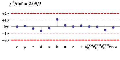
Figure 1: Pictorial representation of the deviation of our predictions from low energy experimental data for the charged lepton Yukawa couplings and quark Yukawa couplings and mixing parameters. The deviations of the charged lepton masses are given in 1% while all other deviations are given in units of standard deviations $\sigma$.

Parameter	Value
$a_{u}$	$-3.01\cdot 10^{-5}$
$b_{u}$	$-2.66\cdot 10^{-4}$
$c_{u}$	$-2.57\cdot 10^{-3}$
$d_{u}$	$3.09\cdot 10^{-2}$
$e_{u}$	$2.05$
$\epsilon_{2}$	$-3.57\cdot 10^{-5}$
$\epsilon_{102}$	$3.17\cdot 10^{-5}$
$\epsilon_{23}$	$1.62\cdot 10^{-4}$
$\epsilon_{3}$	$1.24\cdot 10^{-2}$
$\tan\beta$	$1.49$

Table 4: Values of the effective parameters of the quark and charged lepton Yukawa matrices and $\tan\beta$ for $M_{\text{SUSY}}=750$ GeV. The numerical values are determined from a $\chi^{2}$-fit to experimental data with a $\chi^{2}$ per degree of freedom of 2.05/3.

Quantity (at $m_{t}(m_{t})$)	Experiment	Model	Deviation
$y_{\tau}$ in $10^{-2}$	1.00	$1.00$	$-0.277$
$y_{\mu}$ in $10^{-4}$	5.89	$5.89$	$0.097$
$y_{e}$ in $10^{-6}$	2.79	$2.79$	$-0.016$
$y_{b}$ in $10^{-2}$	$1.58\pm 0.05$	$1.64$	$1.088$
$y_{s}$ in $10^{-4}$	$2.99\pm 0.86$	$2.95$	$-0.226$
$y_{d}$ in $10^{-6}$	$15.9^{+6.8}_{-6.6}$	$11.7$	$-0.639$
$y_{t}$	$0.936\pm 0.016$	$0.939$	$0.159$
$y_{c}$ in $10^{-3}$	$3.39\pm 0.46$	$3.40$	$0.223$
$y_{u}$ in $10^{-6}$	$7.01^{+2.76}_{-2.30}$	$7.59$	$0.209$
$\theta_{12}^{\text{CKM}}$	$0.2257^{+0.0009}_{-0.0010}$	$0.2257$	$0.026$
$\theta_{23}^{\text{CKM}}$	$0.0415^{+0.0011}_{-0.0012}$	$0.0409$	$-0.488$
$\theta_{13}^{\text{CKM}}$	$0.0036\pm 0.0002$	$0.0036$	$-0.002$
$\delta_{\text{CKM}}$	$1.2023^{+0.0786}_{-0.0431}$	$1.1975$	$-0.113$

Table 5: Fit results for the quark Yukawa couplings and mixing and the charged lepton Yukawa couplings at low energy compared to experimental data. The values for the Yukawa couplings are extracted from [43] and the CKM parameters from [44]. Note that the experimental uncertainty on the charged lepton Yukawa couplings are negligible small and we have assumed a relative uncertainty of 1 % for them. The $\chi^{2}$ per degree of freedom is 2.05/3. A pictorial representation of the agreement between our predictions and experiment can be found as well in Fig. 1.

For the RGE running of the Yukawa matrices we have used the REAP package [40] and calculated with it the masses and mixing angles at low energies. Note that we have used the RGEs of the MSSM. Possible RGE effects due to including a variant of the NMSSM are neglected. On the one hand we can expect this effect to be flavour blind leading only to a rescaling of the GUT scale parameters and on the other hand, in the scale-invariant NMSSM for example, the RGE effects come from the coupling $\lambda$ which can be small [41] although $\tan\beta$ given there is preferred to be larger than 10. For small $\tan\beta$ the coupling $\lambda$ has to be rather large to be in agreement with recent Higgs data, see, e.g. [42]. Furthermore, SUSY threshold corrections are negligibly small due to the small $\tan\beta$ and hence are not included in the fit.

For the charged lepton and quark masses and their errors at the top scale $m_{t}(m_{t})$ we have taken the values from [43] and for the CKM parameters the PDG values [44]. Note that the experimental errors for the charged lepton masses are tiny and we have estimated the theoretical uncertainty from higher order effects to 1 %, and we will assume this as their errors instead.

The Yukawa matrices depend on nine real parameters (five from the up-type quarks and four from the down-type quarks and charged leptons). Furthermore we have included $\tan\beta$ as a free parameter in the fit. The unification of the $b$ and the $\tau$ Yukawa coupling at the GUT scale depends strongly on this parameter. On the contrary, the masses and mixing angles depend only very weakly on the SUSY scale which we have therefore fixed to $M_{\text{SUSY}}=750$ GeV.

The fit results are summarised in Figure 1 and Tables 4 and 5. We have fitted ten parameters to thirteen observables with a $\chi^{2}$ of 2.05 and hence we can say that our model describes the data very well. Note that we followed here the strategy of our previous paper [33] where we have found that for Yukawa matrices with negligibly small 1-3 mixings we find the correct value for the CKM phase and the Cabibbo angle $\theta_{C}$ with $\theta_{12}^{d}\approx\epsilon_{2}/\epsilon_{23}\lesssim\theta_{C}$ and $\theta_{12}^{u}\approx b_{u}/c_{u}\approx\theta_{C}/2$ if these two angles have a relative phase difference of 90^∘.

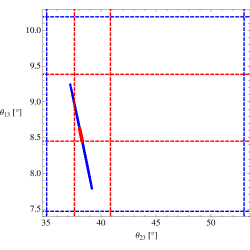
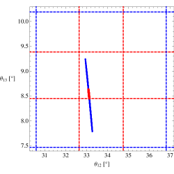
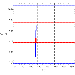
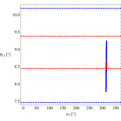
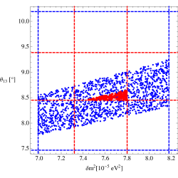
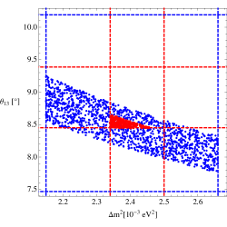
Figure 2: The correlations between $\theta_{13}$ and the other two mixing angles and the two physical phases in PCSD2. The regions compatible with the 1$\sigma$ (3$\sigma$) ranges of the mass squared differences and the mixing angles, taken from [31], are depicted by the red (blue) points and delimited by dashed lines in corresponding colours. The 1$\sigma$ region for the Dirac CP phase is shown in black.

We turn our discussion now to the neutrino sector. Here we did not fit the parameters to the observables because here we are more interested in the allowed ranges and correlations between different observables which help in distinguishing this model from other models.

The effective neutrino mass matrix from eq. (2.1) depends on three parameters. The neutrino mass scale $m_{a}$ the perturbation parameter $\epsilon$ and the relative phase $\alpha$. The phase $\alpha$ in our model is $\pi/3$ as discussed in section 2. Hence, only two real parameters $m_{a}$ and $\epsilon$ completely determine all observables in the neutrino sector.

We have varied these two parameters randomly and the results are shown in Figure 2 where we have used as constraint the fit results of the Bari group [31]. The blue dots agree with all experimental data within 3$\sigma$ while the red dots agree even within 1$\sigma$. The dashed lines in the plots label the corresponding allowed ranges of the observables on the axes. The 1$\sigma$ range of the leptonic Dirac phase $\delta$ is shown in black because it is not measured directly and the fit results should be taken with a grain of salt. In the scan we also did not include it as a constraint.

We are everywhere in good agreement with the experimental data and we find clear correlations. Especially, noteworthy is the value for $\theta_{23}$ which lies around $38.5^{\circ}$. We also make precise predictions for the CP violating phases. One of the Majorana phases is unphysical because one neutrino remains massless. The Dirac CP phase has a value of $\delta\approx 130^{\circ}$ and the physical Majorana phase is $\alpha_{2}\approx 315^{\circ}$. The Jarlskog determinant $J_{\text{CP}}$ is around 0.025 and the effective neutrino mass for neutrinoless double beta decay $m_{ee}$ is of the order of $3\times 10^{-3}$ eV, beyond the reach of current experiments.

7 Summary

We have constructed a unified $A_{4}\times SU(5)$ model featuring the new type of constrained sequential dominance CSD2 proposed recently in [17]. The $A_{4}\times SU(5)$ model, with the CSD2 vacuum alignments $(0,1,1)^{T}$ and $(1,0,2)^{T}$, provides an excellent fit to the present data on quark and lepton masses and mixings, including the measured value of the leptonic mixing angle $\theta_{13}$ from Daya Bay and RENO, with testable predictions for the yet unknown parameters of the leptonic mixing matrix.

The main idea of the present model is that, with a strong normal hierarchical spectrum (with $m^{\nu}_{1}=0$ by construction since there are only two right-handed neutrinos) the 1-3 angle in the neutrino sector, $\theta_{13}^{\nu}$, is related to a ratio of neutrino masses by $\theta_{13}^{\nu}=\frac{\sqrt{2}}{3}\frac{m^{\nu}_{2}}{m^{\nu}_{3}}$, leading to $\theta^{\nu}_{13}\sim 5^{\circ}-6^{\circ}$. In addition, the reactor angle receives another contribution from mixing in the charged lepton sector. The charged lepton mixing induces a correction to $\theta_{13}$ of $\sim 3^{\circ}$ which adds up constructively with $\theta^{\nu}_{13}$ to give

$$\theta_{13}\sim 8^{\circ}-9^{\circ}\;,$$ (7.1)

within the range of the measured value from Daya Bay and RENO. The constructive addition of the neutrino and charged lepton mixing angles is achieved by assuming high energy CP invariance which is spontaneously broken by flavon fields whose phases are controlled using Abelian $\mathbb{Z}_{3}$ and $\mathbb{Z}_{4}$ symmetries as proposed in [22]. We emphasise that in our approach one can either use a “simple” CP symmetry, under which the components of the scalar fields transform trivially as $\phi_{i}\rightarrow\phi_{i}^{*}$, or a “generalised” CP symmetry (see e.g. [27] and references therein) where, in our basis, the triplet fields would transform as $\phi_{i}\rightarrow U_{3}\phi_{i}^{*}$, with $U_{3}$ interchanging the second and third component of a triplet representation.

The resulting unified flavour model is highly predictive, as described in section 6, since only two parameters determine the neutrino mass matrix, while the charged lepton corrections are fixed by the GUT framework: In particular, for the Dirac CP phase $\delta$, for the one physical Majorana CP phase $\alpha_{2}$ and for the atmospheric angle $\theta_{23}$ we obtain the predictions

$$\delta\approx 130^{\circ}\;,\quad\alpha_{2}\approx 315^{\circ}\quad\mbox{and}\quad\theta_{23}\approx 38.5^{\circ}\;.$$ (7.2)

The predictions for $\delta$ and $\theta_{23}$ will be tested by the ongoing and future neutrino oscillation experiments. In addition, for $\theta_{12}$, we predict a value of

$$\theta_{12}\sim 33^{\circ}\;,$$ (7.3)

which is slightly smaller than the tribimaximal mixing value but may be tested by a future reactor experiment with $\sim 60$ km baseline, which could measure $\theta_{12}$ with much improved precision [32]. Furthermore, in the quark sector, we obtain a right-angled unitarity triangle (with $\alpha\approx 90^{\circ}$) from the same vacuum alignment techniques for the phases [22], realizing the phase sum rule of [33].

In summary, we have presented a highly predictive new unified model for fermion masses and mixing, which, in fact, represents the first unified indirect family symmetry model in the literature that has been constructed to date that is consistent with all experimental data on quark and lepton mass and mixing angles, and makes definite predictions for CP phases in both the quark and lepton sectors.

Appendix A Conventions and Notations

In this section we want to summarize briefly our conventions and define some notation used throughout the main text. We will follow mainly the notation of [30]. The only difference is a sign in the Majorana phases.

The Yukawa couplings follow the left-right convention

$$\mathcal{L}_{\text{Yuk}}=-Y_{ij}\overline{\psi_{L}^{i}}\psi_{R}^{j}H+H.c.\,,$$ (A.1)

and for the effective light neutrino mass matrix we use the convention

$$\mathcal{L}_{\nu}=-\frac{1}{2}\bar{L}_{i}(M_{\nu})_{ij}L^{c}_{j}+H.c.\,,$$ (A.2)

where $L$ is the lepton doublet.

In the quark sector we define the CKM matrix by

$$U_{\text{CKM}}=U_{u}U_{d}^{\dagger}=R_{23}U_{13}R_{12}\;,$$ (A.3)

where $U_{u}$ ($U_{d}$) is a unitary matrix diagonalising $Y_{u}Y_{u}^{\dagger}$ ($Y_{d}Y_{d}^{\dagger}$) and

$$U_{12}=\begin{pmatrix}c_{12}&s_{12}\text{e}^{-\operatorname{\text{i}}\delta_{12}}&0\\ -s_{12}\text{e}^{\operatorname{\text{i}}\delta_{12}}&c_{12}&0\\ 0&0&1\end{pmatrix}\;,$$ (A.4)

and similar for $U_{23}$ and $U_{13}$. We use $c_{12}$ and $s_{12}$ as abbreviations for $\cos\theta_{12}$ and $\sin\theta_{12}$. The matrices $R_{23}$ and $R_{12}$ are $U_{23}$ and $U_{12}$ with the complex phases set to zero. In this case $\delta_{13}$ coincides with the CKM phase $\delta_{\text{CKM}}$.

For the PMNS matrix we use

$$U_{\text{PMNS}}=U_{e}U_{\nu}^{\dagger}=R_{23}U_{13}R_{12}\text{ diag}(\text{e}^{-\operatorname{\text{i}}\alpha_{1}/2},\text{e}^{-\operatorname{\text{i}}\alpha_{2}/2},1)\;,$$ (A.5)

where the neutrino mass matrix is diagonalized via

$$U_{\nu}M_{\nu}M_{\nu}^{\dagger}U_{\nu}^{\dagger}=\text{diag}(m_{1}^{2},m_{2}^{2},m_{3}^{2})\;.$$ (A.6)

and $U_{\nu}^{\dagger}=U^{\nu}_{23}U^{\nu}_{13}U^{\nu}_{12}$ (note the Hermitian conjugation). This conventions imply a complex conjugation of the neutrino mass matrix $M_{\nu}$ compared to our previous CSD2 paper [17] and also the sign of the Majorana phases here is different.

Appendix B The Renormalizable Superpotential

	$SU(5)$	$A_{4}$	$U(1)_{R}$	$\mathbb{Z}_{4}$	$\mathbb{Z}_{4}$	$\mathbb{Z}_{3}$	$\mathbb{Z}_{3}$	$\mathbb{Z}_{3}$	$\mathbb{Z}_{3}$
$\Sigma_{1}$, $\bar{\Sigma}_{1}$	$\mathbf{5}$, $\bar{\mathbf{5}}$	$\mathbf{1}$, $\mathbf{1}$	1, 1	2, 2	0, 0	1, 2	2, 1	2, 1	0, 0
$\Sigma_{2}$, $\bar{\Sigma}_{2}$	$\mathbf{5}$, $\bar{\mathbf{5}}$	$\mathbf{1}$, $\mathbf{1}$	1, 1	0, 0	0, 0	2, 1	0, 0	1, 2	0, 0
$\Sigma_{3}$, $\bar{\Sigma}_{3}$	$\mathbf{5}$, $\bar{\mathbf{5}}$	$\mathbf{1}$, $\mathbf{1}$	1, 1	3, 1	3, 1	0, 0	0, 0	2, 1	0, 0
$\Upsilon_{1}$, $\bar{\Upsilon}_{1}$	$\mathbf{10}$, $\overline{\mathbf{10}}$	$\mathbf{3}$, $\mathbf{3}$	1, 1	1,3	3, 1	1, 2	2, 1	2, 1	1, 2
$\Upsilon_{2}$, $\bar{\Upsilon}_{2}$	$\mathbf{10}$, $\overline{\mathbf{10}}$	$\mathbf{3}$, $\mathbf{3}$	1, 1	3, 1	3, 1	0, 0	1, 2	0, 0	1, 2
$\Upsilon_{3}$, $\bar{\Upsilon}_{3}$	$\mathbf{10}$, $\overline{\mathbf{10}}$	$\mathbf{3}$, $\mathbf{3}$	1, 1	3, 1	2, 2	1, 2	1, 2	0, 0	0, 0
$\Xi_{1}$, $\bar{\Xi}_{1}$	$\mathbf{5}$, $\bar{\mathbf{5}}$	$\mathbf{3}$, $\mathbf{3}$	1, 1	3, 1	3, 1	1, 2	1, 2	0, 0	0, 0
$\Xi_{2}$, $\bar{\Xi}_{2}$	$\mathbf{5}$, $\bar{\mathbf{5}}$	$\mathbf{3}$, $\mathbf{3}$	1, 1	3, 1	3, 1	0, 0	1, 2	0, 0	1, 2
$\Xi_{3}$, $\bar{\Xi}_{3}$	$\mathbf{5}$, $\bar{\mathbf{5}}$	$\mathbf{3}$, $\mathbf{3}$	1, 1	3, 1	2, 2	1, 2	1, 2	0, 0	0, 0
$\Omega_{1}$, $\bar{\Omega}_{1}$	$\mathbf{10}$, $\overline{\mathbf{10}}$	$\mathbf{1}$, $\mathbf{1}$	1, 1	3, 1	3, 1	1, 2	2, 1	2, 1	0, 0
$\Omega_{2}$, $\bar{\Omega}_{2}$	$\mathbf{10}$, $\overline{\mathbf{10}}$	$\mathbf{1}$, $\mathbf{1}$	1, 1	3, 1	3, 1	1, 2	0, 0	1, 2	0, 0
$\Omega_{3}$, $\bar{\Omega}_{3}$	$\mathbf{10}$, $\overline{\mathbf{10}}$	$\mathbf{1}$, $\mathbf{1}$	1, 1	3, 1	3, 1	2, 1	2, 1	1, 2	0, 0
$\Gamma_{1}$, $\bar{\Gamma}_{1}$	$\mathbf{1}$, $\mathbf{1}$	$\mathbf{1}$, $\mathbf{1}$	0, 2	0, 0	0, 0	2, 1	0, 0	0, 0	1, 2
$\Gamma_{2}$, $\bar{\Gamma}_{2}$	$\mathbf{1}$, $\mathbf{1}$	$\mathbf{1}$, $\mathbf{1}$	0, 2	0, 0	0, 0	2, 1	0, 0	2, 1	2, 1
$\Gamma_{3}$, $\bar{\Gamma}_{3}$	$\mathbf{1}$, $\mathbf{1}$	$\mathbf{1}$, $\mathbf{1}$	0, 2	0, 0	0, 0	1, 2	2, 1	0, 0	2, 1
$\Gamma_{4}$, $\bar{\Gamma}_{4}$	$\mathbf{1}$, $\mathbf{1}$	$\mathbf{1}$, $\mathbf{1}$	0, 2	0, 0	0, 0	2, 1	1, 2	0, 0	0, 0
$\Gamma_{5}$, $\bar{\Gamma}_{5}$	$\mathbf{1}$, $\mathbf{1}$	$\mathbf{1}$, $\mathbf{1}$	0, 2	0, 0	0, 0	1, 2	0, 0	1, 2	0, 0
$\Gamma_{6}$, $\bar{\Gamma}_{6}$	$\mathbf{1}$, $\mathbf{1}$	$\mathbf{3}$, $\mathbf{3}$	0, 2	0, 0	0, 0	1, 2	2, 1	2, 1	0, 0
$\Gamma_{7}$, $\bar{\Gamma}_{7}$	$\mathbf{1}$, $\mathbf{1}$	$\mathbf{1}$, $\mathbf{1}$	0, 2	2, 2	2, 2	0, 0	0, 0	0, 0	0, 0
$\Gamma_{8}$, $\bar{\Gamma}_{8}$	$\mathbf{1}$, $\mathbf{1}$	$\mathbf{1}$, $\mathbf{1}$	0, 2	0, 0	2, 2	0, 0	0, 0	0, 0	0, 0
$\Gamma_{9}$, $\bar{\Gamma}_{9}$	$\mathbf{1}$, $\mathbf{1}$	$\mathbf{1}$, $\mathbf{1}$	0, 2	0, 0	0, 0	0, 0	1, 2	2, 1	0, 0

Table 6: The messenger field content of our model. Every line represents a messenger pair which receives a mass larger than the GUT scale and no cross terms are allowed. In the main text we labelled the messenger mass scale generically with $\Lambda$.

In this appendix we discuss the full renormalizable superpotential including the messenger fields which after being integrated out give the effective operators as discussed before.

We start with the superpotential bilinear in the fields which is in our case only the mass terms for the messengers

$$\mathcal{W}^{\text{ren}}_{\Lambda}=M_{\Sigma_{i}}\Sigma_{i}\bar{\Sigma}_{i}+M_{\Upsilon_{i}}\Upsilon_{i}\bar{\Upsilon}_{i}+M_{\Xi_{i}}\Xi_{i}\bar{\Xi}_{i}+M_{\Omega_{i}}\Omega_{i}\bar{\Omega}_{i}+M_{\Gamma_{i}}\Gamma_{i}\bar{\Gamma}_{i}\;.$$ (B.1)

The full list of messenger fields is given in Table 6 where every line is a messenger pair which receives a mass larger than the GUT scale so that they can be integrated out to give the desired effective operators. To simplify the notation before we have introduced the messenger scale $\Lambda$ as shorthand which is related to the individual messenger masses with order one coefficients.

Note that in the superpotential bilinear in the fields no $\mu$-term for the Higgs fields appears. This term is forbidden by symmetries and in combination with a NMSSM like mechanism helps to increase the Higgs mass to the experimentally determined value. A possible singlet field $S$ with couplings $S(H_{5}\bar{H}_{5}+H_{45}\bar{H}_{45})$ would not appear anywhere else in the superpotential with the symmetries and field content as specified in Tables  1, 2, 3 and 6.

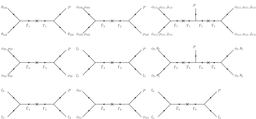
Figure 3: The supergraphs before integrating out the messengers for the flavon sector (only diagrams are shown which give non-renormalizable contributions).

The next step in our discussion of the renormalizable superpotential is the flavon sector. The full potential for this sector reads (dropping for the sake of simplicity order one coefficients)

$$\mathcal{W}^{\text{ren}}_{\text{flavon}} =O_{1;2}\phi_{1}\phi_{2}+O_{1;3}\phi_{1}\phi_{3}+O_{2;3}\phi_{2}\phi_{3}+O_{111;211}\phi_{111}\phi_{211}+O_{111;23}\phi_{111}\phi_{23}$$

$$+O_{23;211}\phi_{23}\phi_{211}+O_{2;102}\phi_{2}\phi_{102}+O_{211;102}\phi_{211}\phi_{102}+O_{1;23}\phi_{1}\phi_{23}$$

$$+A_{1}\phi_{1}\phi_{1}+A_{2}\phi_{2}\phi_{2}+A_{3}\phi_{3}\phi_{3}+A_{111}\left(\phi_{111}^{2}+\phi_{111}\rho_{111}+\tilde{\phi}_{111}\rho_{111}\right)$$

$$+P\Gamma_{9}\xi_{u}+\bar{\Gamma}_{9}\xi_{u}^{2}+P\Gamma_{8}^{2}+\bar{\Gamma}_{8}\phi_{2}^{2}+\bar{\Gamma}_{8}\theta_{2}^{2}+P\Gamma_{7}^{2}+\bar{\Gamma}_{7}(\phi_{111}^{2}+\rho_{111}^{2}+\tilde{\rho}_{111}^{2})$$

$$+P\phi_{211}\Gamma_{6}+\phi_{211}^{2}\bar{\Gamma}_{6}+P\xi_{2}\Gamma_{5}+\xi_{2}^{2}\bar{\Gamma}_{5}+P\xi_{1}\Gamma_{4}+\xi_{1}^{2}\bar{\Gamma}_{4}+P\rho_{23}\Gamma_{3}+(\phi_{23}^{2}+\rho_{23}^{2})\bar{\Gamma}_{3}$$

$$+P\rho_{102}\Gamma_{2}+(\phi_{102}^{2}+\rho_{102}^{2})\bar{\Gamma}_{2}+P\theta_{102}\Gamma_{1}+\theta_{102}^{2}\bar{\Gamma}_{1}\;.$$ (B.2)

The first three lines of this superpotential have already been discussed in the flavon alignment section 4 while the last four lines are needed to fix the phases of the various flavon vevs. For instance, the messenger pair $\Gamma_{1}$ and $\bar{\Gamma}_{1}$ gives after integrating out the effective operator $1/\Lambda P\theta_{102}^{3}$ where in this case $\Lambda$ stands for $M_{\Gamma_{1}}$ multiplied by real order one couplings. This operator fixes the phase of $\langle\theta_{102}\rangle$ up to a discrete choice as discussed before.

We will not list here all of the effective operators because they have already appeared in our superpotential for the flavon alignment and they can also be read off from the diagrams in Figure 3 after contracting the messenger propagators to points.

Figure 4: The supergraphs before integrating out the messengers for the down-type quark and charged lepton sector.

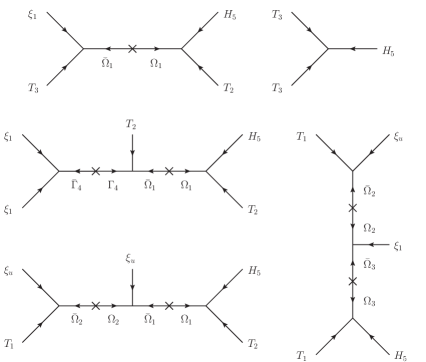
Figure 5: The supergraphs before integrating out the messengers for the up-type quark sector.

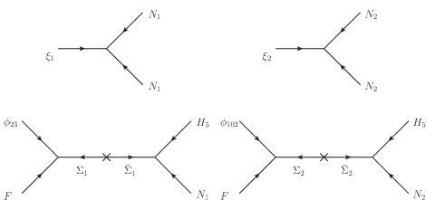
Figure 6: The supergraphs before integrating out the messengers for the neutrino sector.

For the renormalizable couplings including the matter and Higgs fields we find the renormalizable superpotential (again dropping order one coefficients)

$$\mathcal{W}^{\text{ren}}_{d} =T_{3}\bar{H}_{5}\bar{\Sigma}_{3}+F\phi_{3}\Sigma_{3}+T_{2}\phi_{23}\bar{\Upsilon}_{1}+\bar{H}_{45}\Upsilon_{1}\bar{\Xi}_{1}+FH_{24}\Xi_{1}+T_{2}\phi_{102}\bar{\Upsilon}_{2}+\bar{H}_{5}\Upsilon_{2}\bar{\Xi}_{2}$$

$$+\theta_{102}\Xi_{2}\bar{\Xi}_{1}+T_{1}\phi_{2}\bar{\Upsilon}_{3}+\bar{H}_{5}\Upsilon_{3}\bar{\Xi}_{3}+\theta_{2}\Xi_{3}\bar{\Xi}_{1}\;,$$ (B.3)

$$\mathcal{W}^{\text{ren}}_{u} =T_{1}H_{5}\Omega_{3}+\xi_{1}\Omega_{2}\bar{\Omega}_{3}+T_{1}\xi_{u}\bar{\Omega}_{2}+\Omega_{2}\xi_{u}\bar{\Omega}_{1}+T_{2}\Gamma_{4}\bar{\Omega}_{1}$$

$$+\bar{\Gamma}_{4}\xi_{1}^{2}+T_{2}H_{5}\Omega_{1}+T_{3}\xi_{1}\bar{\Omega}_{1}+T_{3}^{2}H_{5}\;,$$ (B.4)

$$\mathcal{W}^{\text{ren}}_{\nu} =\xi_{1}N_{1}^{2}+\xi_{2}N_{2}^{2}+F\phi_{23}\Sigma_{1}+N_{1}H_{5}\bar{\Sigma}_{1}+F\phi_{102}\Sigma_{2}+N_{2}H_{5}\bar{\Sigma}_{2}\;.$$ (B.5)

After integrating out the heavy messenger fields we end up with the non-renormalizable operators as discussed in section 3, cf. also Figures 4-6.

In addition to the renormalizable operators discussed so far there are six more operators allowed by the symmetries which are

$$\mathcal{W}^{\text{ren}}_{\text{neg}}=T_{1}\Gamma_{9}\bar{\Omega}_{1}+T_{2}\Gamma_{9}\bar{\Omega}_{3}+\Xi_{1}\bar{\Xi}_{3}\phi_{2}+\Gamma_{9}\Omega_{1}\bar{\Omega}_{2}+\Gamma_{4}\bar{\Omega}_{2}\Omega_{3}+\Gamma_{1}\Xi_{1}\bar{\Xi}_{2}\;.$$ (B.6)

The first two operators contribute effectively to the $T_{1}T_{2}H_{5}\xi_{u}^{2}$ operator already present and for the sake of simplicity we have not shown them in Figure 5. The third operator generates the dimension six operator $FT_{2}\bar{H}_{45}H_{24}\phi_{2}\phi_{23}$ which gives a contribution to the 2-2 element of the down-type quark and charged lepton Yukawa matrix. In fact the correction has the same phase and the same $SU(5)$ Clebsch–Gordan coefficient as the leading order coefficient so that we can safely neglect it. The last three operators finally give, after integrating out the heavy messengers, dimension seven and eight operators which give only small corrections (in our model we have discussed operators up to dimension six). The dimension seven operators, for instance, are induced by $\Gamma_{9}\Omega_{1}\bar{\Omega}_{2}$ which gives corrections to the $1-3$ and $2-3$ elements of the up-type quark Yukawa matrix which are very small compared to all other elements which are generated at maximum by a dimension five operator.

References

- [1] J. Beringer et al. [Particle Data Group Collaboration], Phys. Rev. D 86 (2012) 010001.
- [2] P. Adamson et al. [MINOS Collaboration], Phys. Rev. Lett. 107 (2011) 181802 [arXiv:1108.0015].
- [3] Y. Abe et al. [DOUBLE-CHOOZ Collaboration], Phys. Rev. Lett. 108 (2012) 131801 [arXiv:1112.6353].
- [4] K. Abe et al. [T2K Collaboration], arXiv:1106.2822.
- [5] F. P. An et al. [DAYA-BAY Collaboration], Phys. Rev. Lett. 108 (2012) 171803 [arXiv:1203.1669]; Y. Wang, talk at What is ? INVISIBLES12 and Alexei Smirnov Fest (Galileo Galilei Institute for Theoretical Physics, Italy, 2012); available at http://indico.cern.ch/conferenceTimeTable.py?confId=195985.
- [6] J. K. Ahn et al. [RENO Collaboration], Phys. Rev. Lett. 108 (2012) 191802 [arXiv:1204.0626].
- [7] M. Ishitsuka, talk at Neutrino 2012 (Kyoto TERRSA, Japan, 2012); available at http://kds.kek.jp/conferenceTimeTable.py?confId=9151.
- [8] P. F. Harrison, D. H. Perkins and W. G. Scott, Phys. Lett. B 530 (2002) 167 [hep-ph/0202074].
- [9] H. -J. He and F. -R. Yin, Phys. Rev. D 84 (2011) 033009 [arXiv:1104.2654 [hep-ph]]; Z.-Z. Xing, arXiv:1106.3244; N. Qin and B. Q. Ma, Phys. Lett. B 702 (2011) 143 [arXiv:1106.3284]; Y. j. Zheng and B. Q. Ma, arXiv:1106.4040; S. Zhou, arXiv:1106.4808; T. Araki, arXiv:1106.5211; N. Haba, R. Takahashi, arXiv:1106.5926; D. Meloni, arXiv:1107.0221; S. Morisi, K. M. Patel and E. Peinado, arXiv:1107.0696; W. Chao, Y.-J. Zheng, arXiv:1107.0738; H. Zhang, S. Zhou, arXiv:1107.1097; X. Chu, M. Dhen, T. Hambye, arXiv:1107.1589; P. S. B. Dev, R. N. Mohapatra, M. Severson, arXiv:1107.2378; R. d. A. Toorop, F. Feruglio, C. Hagedorn, arXiv:1107.3486; S. F. King and C. Luhn, JHEP 1109 (2011) 042 [arXiv:1107.5332 [hep-ph]]; Q. H. Cao, S. Khalil, E. Ma and H. Okada, arXiv:1108.0570; S. F. Ge, D. A. Dicus and W. W. Repko, arXiv:1108.0964; F. Bazzocchi, arXiv:1108.2497; H. -J. He and X. -J. Xu, Phys. Rev. D 86 (2012) 111301 [arXiv:1203.2908 [hep-ph]]; S. F. King, Phys. Lett. B 718 (2012) 136 [arXiv:1205.0506 [hep-ph]].
- [10] S. Antusch and V. Maurer, Phys. Rev. D 84 (2011) 117301 [arXiv:1107.3728 [hep-ph]]; S. Antusch, C. Gross, V. Maurer and C. Sluka, Nucl. Phys. B 866 (2013) 255 [arXiv:1205.1051 [hep-ph]].
- [11] D. Marzocca, S. T. Petcov, A. Romanino and M. Spinrath, JHEP 1111 (2011) 009 [arXiv:1108.0614 [hep-ph]].
- [12] S. F. King, C. Luhn and A. J. Stuart, Nucl. Phys. B 867 (2013) 203 [arXiv:1207.5741 [hep-ph]]; C. Hagedorn, S. F. King and C. Luhn, Phys. Lett. B 717 (2012) 207 [arXiv:1205.3114 [hep-ph]]; I. K. Cooper, S. F. King and C. Luhn, JHEP 1206 (2012) 130 [arXiv:1203.1324 [hep-ph]]; I. de Medeiros Varzielas and G. G. Ross, arXiv:1203.6636 [hep-ph].
- [13] A. Meroni, S. T. Petcov and M. Spinrath, Phys. Rev. D 86 (2012) 113003 [arXiv:1205.5241 [hep-ph]].
- [14] N. Haba, A. Watanabe and K. Yoshioka, Phys. Rev. Lett. 97 (2006) 041601 [hep-ph/0603116]; X. G. He and A. Zee, Phys. Lett. B 645 (2007) 427 [hep-ph/0607163]; W. Grimus and L. Lavoura, JHEP 0809 (2008) 106 [arXiv:0809.0226]; H. Ishimori, Y. Shimizu, M. Tanimoto and A. Watanabe, Phys. Rev. D 83 (2011) 033004 [arXiv:1010.3805]; Y. Shimizu, M. Tanimoto and A. Watanabe, arXiv:1105.2929; X. G. He and A. Zee, arXiv:1106.4359.
- [15] C. S. Lam, Phys. Rev. D 74 (2006) 113004 [hep-ph/0611017]; C. H. Albright and W. Rodejohann, Eur. Phys. J. C 62 (2009) 599 [arXiv:0812.0436]; C. H. Albright, A. Dueck and W. Rodejohann, Eur. Phys. J. C 70 (2010) 1099 [arXiv:1004.2798].
- [16] S. F. King and C. Luhn, JHEP 1109 (2011) 042 [arXiv:1107.5332 [hep-ph]]; I. K. Cooper, S. F. King and C. Luhn, JHEP 1206 (2012) 130 [arXiv:1203.1324 [hep-ph]]; C. Hagedorn, S. F. King and C. Luhn, Phys. Lett. B 717 (2012) 207 [arXiv:1205.3114 [hep-ph]].
- [17] S. Antusch, S. F. King, C. Luhn and M. Spinrath, Nucl. Phys. B 856 (2012) 328 [arXiv:1108.4278 [hep-ph]].
- [18] S. F. King, Phys. Lett. B 439 (1998) 350 [hep-ph/9806440]; S. F. King, Nucl. Phys. B 562 (1999) 57 [hep-ph/9904210]; S. F. King, Nucl. Phys. B 576 (2000) 85 [hep-ph/9912492]; S. F. King, JHEP 0209 (2002) 011 [hep-ph/0204360]; S. Antusch, S. Boudjemaa, S. F. King, JHEP 1009 (2010) 096 [arXiv:1003.5498].
- [19] S. F. King, JHEP 0209 (2002) 011 [hep-ph/0204360]; S. F. King, JHEP 0508 (2005) 105 [hep-ph/0506297].
- [20] S. F. King, Phys. Lett. B 675 (2009) 347 [arXiv:0903.3199].
- [21] K. Harigaya, M. Ibe and T. T. Yanagida, Phys. Rev. D 86 (2012) 013002 [arXiv:1205.2198 [hep-ph]].
- [22] S. Antusch, S. F. King, C. Luhn and M. Spinrath, Nucl. Phys. B 850 (2011) 477 [arXiv:1103.5930 [hep-ph]].
- [23] S. F. King and C. Luhn, arXiv:1301.1340 [hep-ph].
- [24] A detailed review and references can be found in: G. C. Branco, R. G. Felipe and F. R. Joaquim, arXiv:1111.5332 [hep-ph].
- [25] G. G. Ross, L. Velasco-Sevilla and O. Vives, Nucl. Phys. B 692 (2004) 50 [hep-ph/0401064].
- [26] S. F. King and M. Malinsky, Phys. Lett. B 645 (2007) 351 [hep-ph/0610250].
- [27] F. Feruglio, C. Hagedorn and R. Ziegler, arXiv:1211.5560 [hep-ph]; M. Holthausen, M. Lindner and M. A. Schmidt, arXiv:1211.6953 [hep-ph].
- [28] H. Georgi and C. Jarlskog, Phys. Lett. B 86 (1979) 297.
- [29] S. Antusch and S. F. King, Phys. Lett. B 631 (2005) 42 [hep-ph/0508044].
- [30] S. Antusch, S. F. King and M. Malinsky, Nucl. Phys. B 820 (2009) 32 [arXiv:0810.3863 [hep-ph]].
- [31] G. L. Fogli, E. Lisi, A. Marrone, D. Montanino, A. Palazzo and A. M. Rotunno, Phys. Rev. D 86 (2012) 013012 [arXiv:1205.5254 [hep-ph]].
- [32] H. Minakata, H. Nunokawa, W. J. C. Teves and R. Zukanovich Funchal, Phys. Rev. D 71 (2005) 013005 [hep-ph/0407326]; A. Bandyopadhyay, S. Choubey, S. Goswami and S. T. Petcov, Phys. Rev. D 72 (2005) 033013 [hep-ph/0410283].
- [33] S. Antusch, S. F. King, M. Malinsky and M. Spinrath, Phys. Rev. D 81 (2010) 033008 [arXiv:0910.5127 [hep-ph]].
- [34] S. Antusch and M. Spinrath, Phys. Rev. D 79 (2009) 095004 [arXiv:0902.4644 [hep-ph]].
- [35] S. Antusch and M. Spinrath, Phys. Rev. D 78 (2008) 075020 [arXiv:0804.0717 [hep-ph]].
- [36] A. Juttner [on behalf of the FLAG Collaboration], arXiv:1109.1388 [hep-ph].
- [37] G. Aad et al. [ATLAS Collaboration], Phys. Lett. B 716 (2012) 1 [arXiv:1207.7214 [hep-ex]]; S. Chatrchyan et al. [CMS Collaboration], Phys. Lett. B 716 (2012) 30 [arXiv:1207.7235 [hep-ex]].
- [38] U. Ellwanger, C. Hugonie and A. M. Teixeira, Phys. Rept. 496 (2010) 1 [arXiv:0910.1785 [hep-ph]].
- [39] J. C. Callaghan and S. F. King, arXiv:1210.6913 [hep-ph].
- [40] S. Antusch, J. Kersten, M. Lindner, M. Ratz and M. A. Schmidt, JHEP 0503 (2005) 024 [hep-ph/0501272].
- [41] K. Kowalska, S. Munir, L. Roszkowski, E. M. Sessolo, S. Trojanowski and Y. -L. S. Tsai, arXiv:1211.1693 [hep-ph].
- [42] T. Cheng, J. Li, T. Li and Q. -S. Yan, arXiv:1304.3182 [hep-ph]; N. D. Christensen, T. Han, Z. Liu and S. Su, arXiv:1303.2113 [hep-ph].
- [43] Z.-z. Xing, H. Zhang, S. Zhou, Phys. Rev. D77 (2008) 113016. [arXiv:0712.1419 [hep-ph]].
- [44] K. Nakamura et al. (Particle Data Group), J. Phys. G 37 (2010) 075021.
- [45] H. Leutwyler, Nucl. Phys. Proc. Suppl. 94 (2001) 108-115. [hep-ph/0011049].