Spitzer Transits of the Super-Earth GJ1214b and Implications for its Atmosphere

Abstract

We observed the transiting super-Earth exoplanet GJ1214b using Warm Spitzer at 4.5 $\mu$m wavelength during a 20-day quasi-continuous sequence in May 2011. The goals of our long observation were to accurately define the infrared transit radius of this nearby super-Earth, to search for the secondary eclipse, and to search for other transiting planets in the habitable zone of GJ1214. We here report results from the transit monitoring of GJ1214b, including a re-analysis of previous transit observations by Désert et al. (2011). In total, we analyse 14 transits of GJ1214b at 4.5 $\mu$m, 3 transits at 3.6 $\mu$m, and 7 new ground-based transits in the I+z band. Our new Spitzer data by themselves eliminate cloudless solar composition atmospheres for GJ1214b, and methane-rich models from Howe & Burrows (2012). Using our new Spitzer measurements to anchor the observed transit radii of GJ1214b at long wavelengths, and adding new measurements in I+z, we evaluate models from Benneke & Seager (2012) and Howe & Burrows (2012) using a $\chi^{2}$ analysis. We find that the best-fit model exhibits an increase in transit radius at short wavelengths due to Rayleigh scattering. Pure water atmospheres are also possible. However, a flat line (no atmosphere detected) remains among the best of the statistically acceptable models, and better than pure water atmospheres. We explore the effect of systematic differences among results from different observational groups, and we find that the Howe & Burrows (2012) tholin-haze model remains the best fit, even when systematic differences among observers are considered.

1 Introduction

The mass and radius of the nearby transiting super-Earth GJ1214b (Charbonneau et al., 2009) imply that it must have a significant atmosphere (Rogers & Seager, 2010). That inference motivated an extensive effort to detect the atmosphere, by seeking wavelength variations of the transit depth. A wide variety of compositions are possible for super-Earth atmospheres (Miller-Ricci & Fortney, 2010; Benneke & Seager, 2012; Howe & Burrows, 2012), from hydrogen-dominated to heavy-element-rich. Most current observations of the transits (Bean et al., 2010, 2011; Crossfield et al., 2011; Désert et al., 2011; Berta et al., 2011, 2012; de Mooij et al., 2012) have rejected hydrogen-dominated atmospheres for GJ1214b, but Croll et al. (2011) concluded in favor of a low molecular weight atmosphere. The infrared (IR) spectral region is particularly important for such studies, because strong water vapor bands increase the transit depth in the IR significantly as compared to the optical. This is especially true for hydrogen-dominated atmospheres, because of the increased atmospheric scale height. The intrinsically strong IR water vapor opacity makes hydrogen-dominated atmospheres opaque in the IR over several scale heights, in spite of their relative paucity of heavy elements. Also, strong bands of methane and carbon monoxide fall within the Warm Spitzer bandpasses at 3.6- and 4.5 $\mu$m, respectively. Considering that GJ1214b’s M-dwarf host star is bright in the IR, transit observations of GJ1214b using Warm Spitzer become particularly relevant to the characterization of its atmosphere.

In May 2011, we observed the GJ1214 system quasi-continuously for 20 days, using Spitzer’s IRAC instrument at 4.5 $\mu$m. Our investigation had three goals: 1) to improve the transit parameters of the system and constrain the properties of the planet’s transmission spectrum, 2) to search for the secondary eclipse, and 3) to search for other transiting planets in this system, to the outer edge of the habitable zone.

Our observations included minor interruptions for data downloads. But, an unplanned 42-hour data loss also occurred during the 20-day sequence, caused by a combination of spacecraft and Deep Space Network (DSN) downlink anomalies. We therefore re-observed GJ1214 for an additional 42-hours in November, 2011, using the IRAC 3.6 $\mu$m band. Consequently, we have multiple transits at both Warm Spitzer wavelengths, and these data provide a particularly powerful constraint on the IR transit depth. Moreover, since our 4.5 $\mu$m transits were observed nearly consecutively, we have an excellent basis for evaluating the degree to which stellar activity (e.g., star spots) affect the inferred transit depth.

A global analysis of these GJ1214 data is being published by Gillon et al. (2012), including a search for other transiting planets in this system. In this paper, we focus on the implications of our observations for understanding the nature of GJ1214b’s atmosphere, and we investigate the wavelength-dependent transit radius of GJ1214b in detail. Our analysis includes the degree to which star spots - even those not occulted by the planet - contribute to possible bias in the measured radius of the planet. Anchored by our improved precision for these infrared transits of GJ1214b, we add 7 new ground-based transits in the I+z band, and we re-analyze the totality of published wavelength-dependent transit depths for GJ1214b, exploiting recent advances in super-Earth model atmospheres (Benneke & Seager, 2012; Howe & Burrows, 2012).

Sec. 2 describes the details of our observations, and Sec. 3 explains our procedure to extract precise photometry from the data. In Sec. 4 we fit to the photometry, extracting the transit radius for the planet in the warm Spitzer and I+z bands, and we derive improved system parameters. Sec. 5 considers the possible effect of star spots on our results. Sec. 6 discusses implications for the atmosphere of GJ1214b.

2 Observations

2.1 Spitzer

We observed GJ1214 for 20 consecutive days using Warm Spitzer at 4.5 $\mu$m, beginning on April 29, 2011 at 03-46 UTC. We used subarray mode with an exposure time of 2 seconds per frame. The observations contain several $\sim 3$-hour interruptions for data download, and one unanticipated 42-hour gap where data were irretrievably lost. The data loss occurred because the DSN incurred anomalous delays in downloading data at that time. When the Spitzer observatory was designed, long observing campaigns of exoplanet photometry were not envisioned. Spitzer’s onboard flight software was designed to automatically delete data after a certain period of time, to make room in memory for new observations. The DSN anomaly consequently caused the onboard software to delete data before downlink (the flight software has now been corrected so that this will not recur).

To compensate for the data loss, we were awarded 42 hours of continuous observations that began on November 6, 2011, at 11-54 UTC. We elected to acquire these data in Spitzer’s 3.6 $\mu$m bandpass, to complement the 4.5 $\mu$m data from May 2011. We again used 2-second exposure times in subarray mode. In total, our data comprise 791,808 exposures at 4.5 $\mu$m, and 74,624 exposures at 3.6 $\mu$m.

2.2 TRAPPIST

In order to help define the possible effects of stellar activity on the Spitzer transits, to further cross-check our analysis versus Gillon et al. (2012), and to add additional information relevant to the atmosphere of GJ1214b, we observed 7 transits using the TRAPPIST facility (Gillon et al., 2011; Jehin et al., 2011), over the period 2011 March 11 - May 18. The TRAPPIST observations and photometry are described by Gillon et al. (2012), but we summarize the data here. The observations were made using the 60-cm robotic telescope in a slightly defocused mode. An I+z filter gave transmission from 750 to 1100 nm. Differential photometry on the 25-sec exposure images was done (by M.G.) using IRAF/DAOPHOT. In our analysis, we use the same version of the photometry as Gillon et al. (2012), but we perform an independent analysis and transit fitting.

3 Spitzer Photometry

3.1 Aperture Photometry

Our analysis utilizes the Basic Calibrated Data (BCD) files produced by version S18.18.0 of the Spitzer pipeline. Two dimensional (2D) Gaussian centering produces the least scatter in our final photometry (Stevenson et al., 2010; Agol et al., 2010). Knutson et al. (2012) found that flux-weighted centering gives superior results for Spitzer data in studies of exoplanetary phase curves over long time scales. We tried flux-weighted centering for our transit analysis, but it did not result in significant improvement over our 2D Gaussian centering.

In the case of the 4.5 $\mu$m photometry we center a circular aperture of constant radius on the star. We calculate the stellar flux within the aperture, including analytic approximations for the partial coverage of pixels at the boundary of the aperture. We vary the radius of the aperture from 2.0 to 5.0 pixels, in 0.5-pixel increments, and thereby produce seven versions of the photometry at each wavelength. After decorrelation (see below), we chose to use an aperture radius of 2.5 pixels for 4.5 $\mu$m, based on the global scatter in the decorrelated photometry.

In the case of the 3.6 $\mu$m photometry, we examined constant radius photometry– for the same seven radii as in the 4.5 $\mu$m section– and variable radius aperture photometry. The variable radius photometry improves the precision by 41% over constant aperture photometry by varying the aperture radius as a function of the ‘noise-pixel’ calculations per frame (Mighell, 2005; Knutson et al., 2012; Lewis et al., 2013). Therefore we adopt the noise pixel method for our 3.6 $\mu$m photometry, and subsequent intra-pixel decorrelation (see below).

The noise pixel method estimates the effective width of the pixel response function, accounting for undersampling, by calculating the variance of the flux per frame, weighted by the square of the mean flux:

$$\tilde{\beta}_{i}=\frac{\left(\Sigma I_{j}\right)^{2}}{\Sigma\left(I_{j}\right)^{2}},$$ (1)

where $\tilde{\beta}_{i}$ is the noise pixel parameter for the stellar image in frame $i$, $I_{j}$ is the intensity of pixel $j$, and the summations extend over all pixels wherein the stellar intensity is significant. Using the $\sqrt{\tilde{\beta}_{i}}$ as the aperture radius collects an optimum amount of light for photometry. The average aperture radius from using this formulation on our 3.6 $\mu$m data is 2.60 pixels.

3.2 Decorrelation

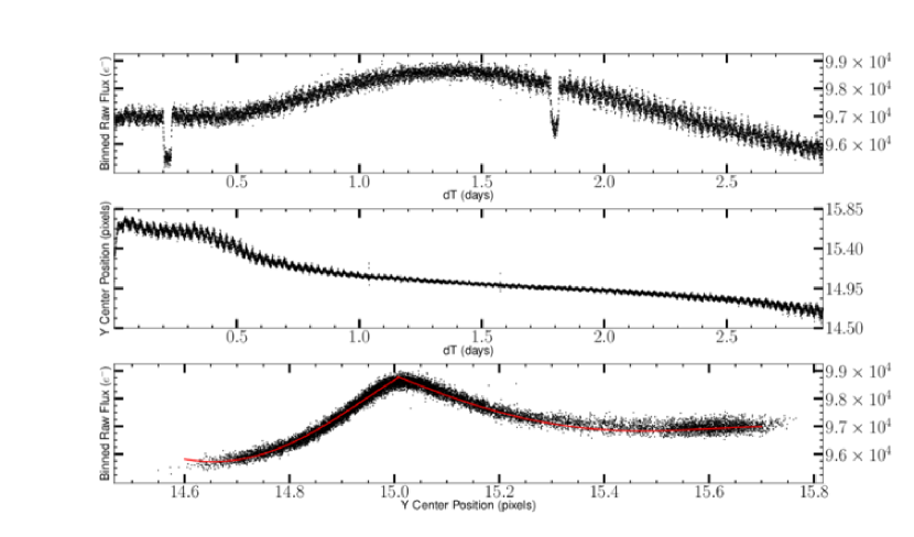
Figure 1: The top panel illustrates raw data for the first 2.9-day portion of our 4.5 $\mu$m photometry, containing two transits. Each data point is aperture photometry before decorrelation, binned by every 10 data points. The middle panel shows the Y-center position as a function time; that which we correlate with the flux to remove the intra-pixel effect, and related systematic noise sources. The lower panel shows the same photometric values, except with the transit regions excluded, plotted versus the Y-pixel position of the stellar image. Note the different spatial dependence of the photometry on each side of pixel center. The red curves are the 4th order polynomial fits that we use to initiate the decorrelation process (see text).

Upon producing photometry, we immediately see Spitzer’s well-known intra-pixel sensitivity effect, that must be decorrelated and removed from the data. A portion of the raw 4.5 $\mu$m photometry (before decorrelation) is illustrated in Figure 1. Because the transits of GJ1214b are substantially larger than the intra-pixel signature, we first mask off the transits from the first stage of decorrelation. Our 4.5 $\mu$m data comprise seven distinct re-acquisitions of GJ1214, with interruptions for data download. Therefore our first stage of decorrelation is done separately for each of the seven re-acquisitions. That inital decorelation fits two polynomials to the data for each re-acquisition. (There are seven sections of the data defined by the data downloads and re-acquisitions.) One polynomial fit is applied to those data points wherein the image centroid lies at Y-coordinate greater than the center of the pixel, and another polynomial fit is applied to those data wherein the image lies at Y-coordinate less than the center of the pixel. Our rationale for this two-parameter fit is based on visual inspection of the photometry, that shows different behavior above the center-of-pixel than below center (see lower panel of Figure 1). The polynomials are fourth order in Y and second order in X, because the photometric variations as a function of Y are more pronounced than with X. Also, visual examination of the variation with Y indicated that lower order polynomials (e.g., quadratic) would not represent the variations optimally. After finding the best fit polynomials, we divide them into the data, including the in-transit data. We only used this step to determine initial conditions for an iterative weighting function method (see below).

We follow the polynomial decorrelation with a second procedure that is itself a two-pass iterative process. We first remove a preliminary transit model from the polynomial-decorrelated data, and apply a Gaussian weighting function (Ballard et al., 2010; Lewis et al., 2013; Knutson et al., 2012) to correct the intra-pixel signatures.

The kernel of the Gaussian weighting uses a $\sigma$ of 0.005 pixels in Y, and 0.01 pixels in X for the 4.5 $\mu$m data, that we determined by trial and error - evaluating the noise level of the final decorrelated photometry. A separate Gaussian weighting was applied to each section of the data between downloads, but the same kernel size was used for all data sections at 4.5 $\mu$m.

For the 3.6 $\mu$m data, we applied a noise-pixel, Gaussian weighting function that uses a variable $\sigma$ in $Y$, $X$, and $\tilde{\beta}$ (noise-pixel value). This varied the weights in the Gaussian kernel to accommodate the necessary number of neighboring points that influence the strength of the correlation between center position and flux, as discussed in Lewis et al. (2013) and Knutson et al. (2012).

Because of effects near the pixel boundary, we chose to subdivide the 3.6 $\mu$m data into 2 sections, encompassing the 2 transits in the data. The pixel boundary effects occured well out of phase of both transits. After examining the global scatter and $\sigma~{}vs.~{}N^{-0.5}$ (bin size) slope residuals, we found that decorrelating after subdividing the 3.6 $\mu$m data set to within $\pm 0.05$ of each transit produced the best noise levels, and resulted in more conservative uncertainty estimates on the transit parameters, by $\sim 10$%. Moreover, this phase range coincides with similar subdivisions in the 4.5 $\mu$m data.

After dividing by the results of the Gaussian weighting, we solve for and subtract an improved transit model, and again apply a second stage weighting function decorrelation. We experimented with a third iteration of this process, but it did not produce significant improvement. Unlike the first (polynomial) stage of decorrelation, the Gaussian weighting function was applied to the totality of the data (i.e., all re-acquisitions) using a single Gaussian kernel. The initial polynomial stage of the decorrelation process may seem unnecessary, since the weighting function alone could remove structure in the data on both large and small spatial scales. However, we find that the polynomials speed up the iterative process by providing a fast start to the iteration. Our final photometry has a standard deviation of $3.7\times 10^{-3}$, which is only 15% greater than the photon noise. Moreover, red noise is minimal and the precision for binned data improves nearly as the square-root of the bin size, as we demonstrate below.

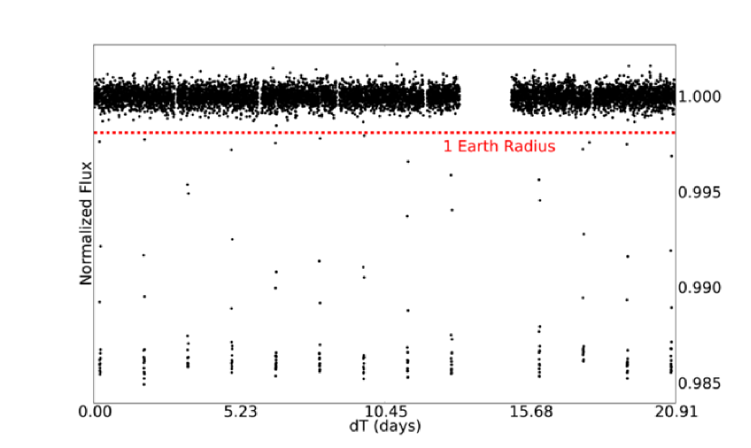
Figure 2: Overview of our 4.5 $\mu$m photometry, after decorrelation and binned in 100 two-second exposures per plotted point. The dashed line shows the transit depth that corresponds to one Earth radius. The 13 transits of GJ1214b are apparent. See Gillon et al. (2012) for an analysis of other possible transiting planets in this system.

Figure 2 shows an overview of our 4.5 $\mu$m photometry, after decorrelation; more detailed depictions are discussed and shown below.

4 Model Fitting for Transit Parameters

We analyze all available Sptizer transits, including a re-analysis of the transits reported by Désert et al. (2011), and TRAPPIST transits using the I+z filter (Gillon et al., 2012). We use three methodologies to determine the best-fit transit parameters for each dataset and wavelength. All three methods use only the data within a phase interval of $\pm 0.05$ around the center of each transit– except for the TRAPPIST transits, which used all of the available data from Gillon et al. (2012).

The first method solves for the best-fit transit parameters of all transits simultaneously at each wavelength. The second method fits each transit individually and independently, then calculates the average of the transit parameters at each wavelength, weighting the individual results by the inverse of their variance. The third method phases and bins all of the transits at each wavelength into a single transit, and fits to those phased & binned data. All 3 methods included a total of 3 transits at 3.6 $\mu$m, 14 transits at 4.5 $\mu$m, and 7 transits in the I+z band. Comparing these three methods gives an indication of the consistency of our results, and we do indeed find good consistency, as noted below.

We now describe the details of those fitting procedures.

4.1 Spitzer 4.5 $\mu$m Transits

We use the formulation of Mandel & Agol (2002) to generate transit curves and fit them to the observed data, thereby extracting the essential parameters of the transit. The 14 Spitzer transits at 4.5 $\mu$m comprise our most extensive and highest quality data. Our simultaneous fit holds the orbital period fixed at the value measured by Bean et al. (2011) $\left(1.58040481\pm 1.210^{-7}\right)$, and uses a Levenberg-Marquardt algorithm to minimize the $\chi^{2}$ for each transit. Although we are minimizing $\chi^{2}$, we do not accept that particular set of transit parameters as our best-fit values. Instead, we explore parameter space using a Markov Chain Monte Carlo (MCMC) method, and also using a residual-permutation (‘prayer-bead’) method. Our best-fit values are taken from the medians of the posterior distributions generated in this exploration of parameter space (see Sec. 4.4).

Our fit extracts a correction to the transit center time (as might be caused by ephemeris error), as well as $a/R_{*}$, $i$, $R_{p}/R_{*}$, and a linear limb-darkening coefficient. We hold the quadratic limb darkening coefficient at zero because Bayesian Information Criterion (Liddle, 2007) analysis supports a linear law, which gives an adequate account of the minimal limb darkening that is characteristic of infrared transits. Moreover, our derived linear limb darkening coefficients at 3.6 and 4.5 microns (c0 =0.158 and 0.128 respectively, see Table 4) are reasonably consistent with the values predicted by Claret & Bloemen (2011) (c0= 0.147 and 0.155) for a model atmosphere having T=3500K (that temperature being their closest match to GJ1214).

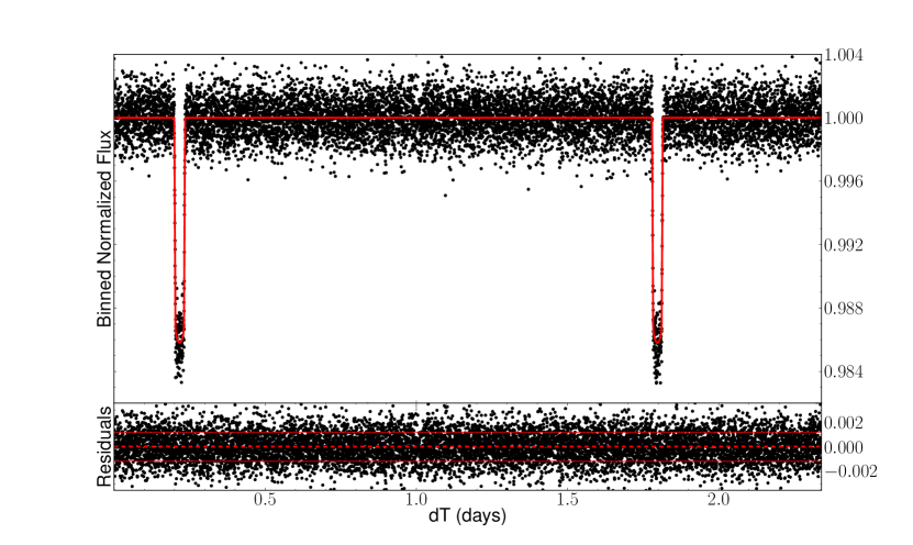
Figure 3: Expansion of a two-transit portion of the 4.5 $\mu$m photometry (Figure 2), with the best-fit transit curves overlaid, binned by every 10 data points. The red lines in the lower panel show a $\pm 1\sigma$ envelope.

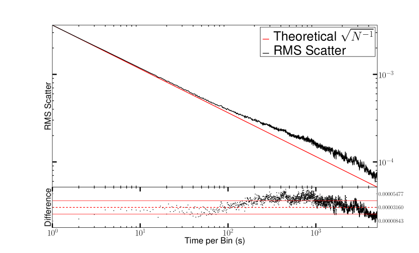
Figure 4: Standard deviation of the residuals (data minus the ‘simultaneous’ fit, in units of the stellar flux) for all 14 transits at 4.5 $\mu$m, versus bin size. The red lines in the lower panel show a $\pm 1\sigma$ envelope.

Figure 3 zooms in on a portion of the simultaneous fit for the first two 4.5 $\mu$m transits, and Figure 4 shows the standard deviation of residuals (data minus simultaneous fit) when binned over different time intervals. Note that we find very little red noise in these data, indicating the success of our multi-stage intra-pixel decorrelation. Note also that our decorrelation process will tend to remove slow variations in the stellar brightness. Hence the apparently constant flux seen in Figure 2 should not be interpreted as evidence for stellar quiesence. (The possible effects of stellar activity on our results are discussed in Sec. 5).

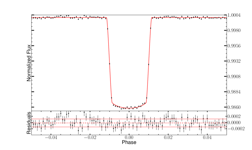
Figure 5: Phased & binned transit of GJ1214b at 4.5 $\mu$m from our 13 Spitzer transits, plus the transit observed by Désert et al. (2011).

In addition, we bin all 14 4.5 $\mu$m transits, including that of Désert et al. (2011), into bins of width $0.001$ in phase, using a running standard deviation for the weights in a weighted mean– phasing them all to a common epoch determined from the simultaneous fit. As before, we include only data within a phase range $\pm 0.05$ of transit center, and we fit to the phased & binned transit using the same Levenberg-Marquardt algorithm described above. Figure 5 shows the resulting fit in comparison to the phased & binned data.

The best-fit Spitzer transit parameters for each 4.5 $\mu$m transit fitted individually are given in Table 1; the individual 3.6 $\mu$m transits (Sec. 4.2) are given in Table 2, and the individual TRAPPIST results (Sec. 4.3) are given in Table 3. Results using the combining methods are summarized in Sec. 4.5.

4.2 Spitzer 3.6 $\mu$m Transits

Our 42-hour ‘replacement’ observations contain two transits at 3.6 $\mu$m, one near the beginning of these data and one near the end. The photometry for these transits was decorrelated using the same methodology described above for 4.5 $\mu$m. In contrast to the 4.5 $\mu$m case, our 3.6 $\mu$m photometry exhibits noticeable red noise. Fortunately, this red noise is most significant in the long interval between the two transits. We limited the effect of this red noise by limiting the range of the data included in our decorrelations and fits. The omitted data did not occur near the transits, nevertheless we tried to develop objective criteria for the range of data that were used.

After comparing the $\sigma~{}vs.~{}N^{-0.5}$ and global $\sigma$, or RMS scatter, of various sized data slices, we determined that trimming the 3.6 $\mu$m data set into a phase range of $\pm 0.05$ around the center of each transit minimized the RMS scatter and the residual of the $\sigma~{}vs.~{}N^{-0.5}$ slope, which minimized the red noise for these transits; and was fortuitously the same range as the $\pm 0.05$ in phase that we adopted for our 4.5 $\mu$m fits.

We repeated all of the methodology described in this section on the Désert et al. (2011) 3.6 $\mu$m transit data, and we found that the slope of $\sigma~{}vs.~{}N^{-0.5}$ was insensitive to the range of data analyzed. As a result, we use the entire Désert et al. (2011) 3.6 $\mu$m data set.

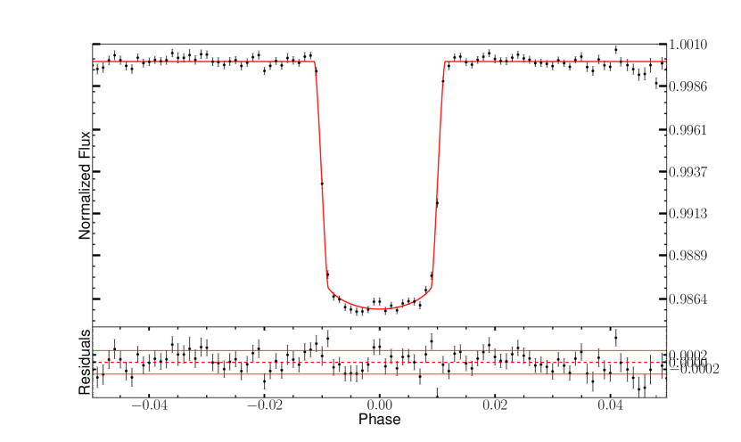
Figure 6: Phased & binned transit of GJ1214b at 3.6 $\mu$m from our two Spitzer transits, plus the transit observed by Désert et al. (2011).

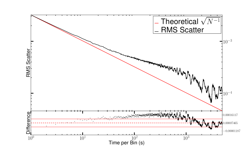
Figure 7: Standard deviation of the residuals (data minus the ‘simultaneous’ fit, in units of the stellar flux) for our two transits at 3.6 $\mu$m plus the Désert et al. (2011) transit, versus bin size. The extra scatter in this figure, compared to Figure 4 above, is related to the number of data points binned overall. There are almost an order of magnitude less points at 3.6 $\mu$m than 4.5 $\mu$m.

As in the 4.5 $\mu$m case, we fit to all 3 of the 3.6 $\mu$m transits using 3 methods: simultaneously, individually, and phased & binned. Figure 6 shows all 3 of the 3.6 $\mu$m transits phased & binned, overlaid with a best-fit curve. Figure 7 illustrates the standard deviation of the 3.6 $\mu$m residuals as a function of bin size for our fits to the simultaneous transit parameters.

4.3 TRAPPIST I+z Transits

For the TRAPPIST data set, we used all 7 distinct epochs of the GJ1214b transiting system provided by Gillon et al. (2012). Three of these epochs overlapped with the Spitzer 4.5 $\mu$m data set. Gillon et al. (2012) used the I+z filter on the TRAPPIST telescope because it supplied a near uniform filter profile from 0.7 - 1.0 $\mu$m.

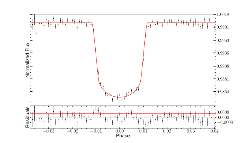
Figure 8: Phased & binned transit of GJ1214b in the I+z band, from TRAPPIST, observed by Gillon et al. (2012).

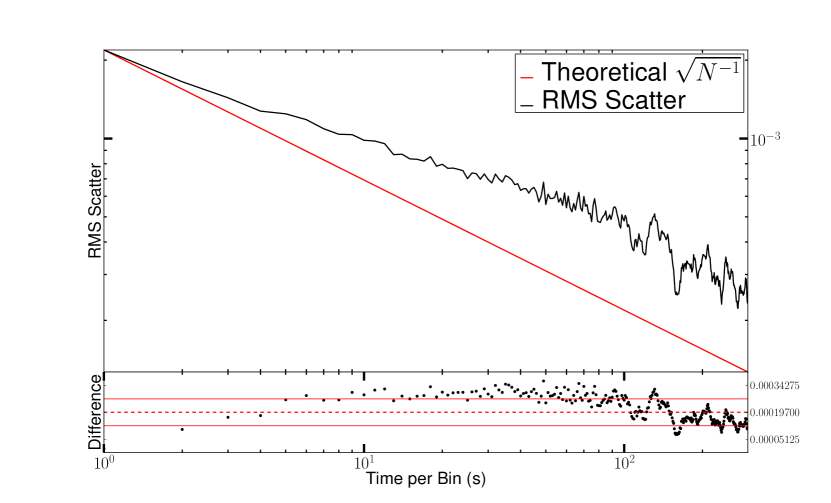
Figure 9: Standard deviation of the residuals (data minus the ‘simultaneous’ fit, in units of the stellar flux) for our seven transits in the I+z band on TRAPPIST. The extra scatter in this figure, compared to Figure 4 & 7 above, is related to the number of data points binned overall. We were only able to bin out to 300 data points ber bin because the most extensive TRAPPIST transit comprised 300 data points.

We determined the physical parameters using all three methods discussed above: a simultanous fit, individual fits, and a fit to phased & binned data. Similar to the Spitzer data sets, we fit a Mandel & Agol (2002) transit model using a Levenberg-Marquardt routine. In contrast to the Spitzer data sets, we fit the TRAPPIST data using a Mandel & Agol (2002) model that included quadratic limb darkening, which accounted for the excess stellar limb-darkening observed in the shorter wavelength transit data. The fit to the phased & binned TRAPPIST data is shown as Figure 8. To analyze the quality of the fit, Figure 9 shows the $\sigma~{}vs.~{}N^{-0.5}$ for the simultaneous fit of the TRAPPIST data set.

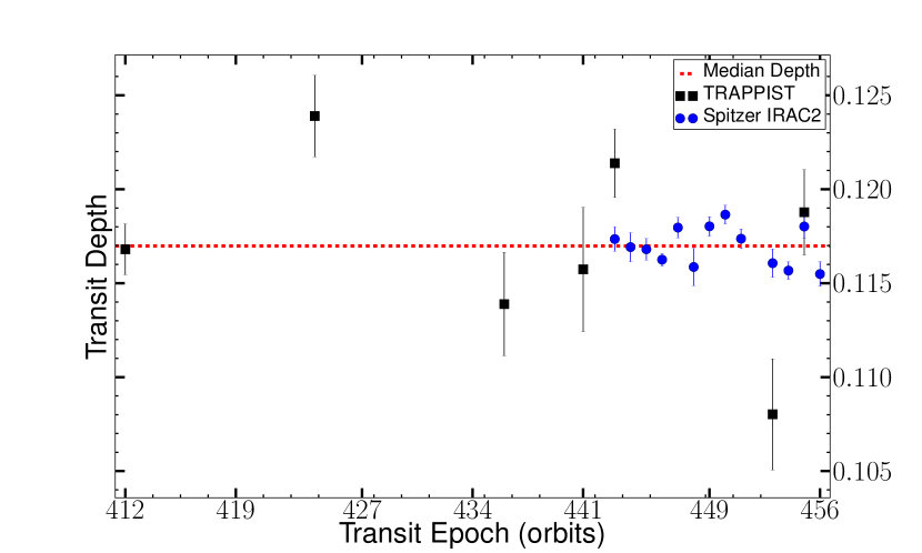
Figure 10: Ratio of planet to stellar radius versus epoch for our 4.5 $\mu$m transits, shown in comparison to transits from TRAPPIST. The red dotted line shows the median value of our 4.5 $\mu$m transits.

The results for the planet-to-star radius ratios, and related error bars, in the I+z band are plotted on Figure 10 for comparison to our 13 Spitzer transits at 4.5 $\mu$m, and listed in Tables 3 & 4. Further information about the data reduction process for the TRAPPIST data set is included in Gillon et al. (2012).

4.4 Errors

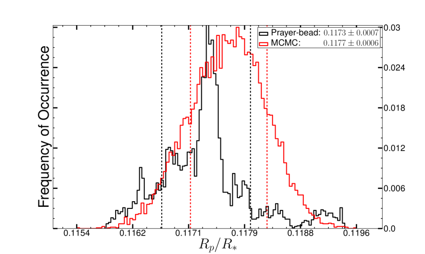
Figure 11: Histograms (posterior distributions) of ${R_{p}}/{R_{*}}$ for the individual fit to the first of our 4.5 $\mu$m transits, showing results from both the MCMC and prayer-bead methods; with dashed lines for the 1$\sigma$ threshold of each distribution.

We used two methods to estimate uncertainties for our derived transit parameters: MCMC and prayer-bead. In both methods the errors - as well as the best-fit values - follow from the posterior distributions. We adopted the prayer-bead method for our quoted results because it explicitly includes the effect of red noise (Désert et al., 2011b). Figure 11 shows the distributions for $R_{p}/R_{*}$ for one of our 4.5 $\mu$m individual fits, showing a broader distribution for the prayer-bead method.

In implementing the prayer-bead method, we permute the residuals only within the adopted phase range of the fit ($\pm 0.05$ in phase). At each permutation, we find the best-fit transit parameters using the Levenberg-Marquardt method, and we add those best-fit values to the posterior distributions of each parameter. We adopt the median of the posterior distribution as the best fit value, following Désert et al. (2011b).

A potential additional source of error is associated with the decorrelation, that is not explicitly propagated into the stage of fitting the photometry. However, we are not concerned about this for two reasons. First, the 4.5 $\mu$m data are so extensive, and the intra-pixel effect is so modest at that wavelength, that we believe those errors in decorrelation have negligible effect. Second, our procedure accounts for imperfect decorrelation at both Spitzer wavelengths, in an implicit fashion. Imperfections in decorrelation create red noise, and that red noise contributes to errors on the derived transit parameters using the prayer-bead method.

In addition to random error, systematic differences may exist between our results and other investigators. We discuss one source of possible systematic difference in Sec. 4.5; the implications of these differences for the nature of GJ1214b’s atmosphere is discussed in Sec. 6.

4.5 System Parameters

As noted above, we estimated the system parameters using three methods: 1) simultaneous fitting of all transits at a given wavelength, 2) averaging system parameters from the individual fits to each transit at a given wavelength, and 3) fitting to phased & binned combinations of transits at a given wavelength. We included the transits observed by Désert et al. (2011) in all three methods. We also fit the TRAPPIST transits using all three methods (see Table 4). Table 1 lists the individual fits to the 4.5 $\mu$m data; Table 2 gives the individual fit results at 3.6 $\mu$m and Table 3 lists the individual fit results for the TRAPPIST transits in the I+z band.

Since our different fitting methods (summarized in Table 4) are simply different ways of accounting for the same data, they should give consistent results as far as the best-fit parameters are concerned. Beyond best-fit consistency, we find that comparison of these methods can provide a basis for caution concerning the errors on the derived parameters. For example, our 4.5 $\mu$m results from the simultaneous fit give ${R_{p}}/{R_{*}}=0.11710\pm 0.00017$, whereas averaging the individual fits, weighted by the inverse of their variances, gives ${R_{p}}/{R_{*}}=0.11699\pm 0.00026$. Although the best-fit values agree well, the larger error from averaging the individual fits may indicate potential variations from transit-to-transit.

Table 5 summarizes our results for the ${R_{p}}/{R_{*}}$ parameter that potentially reveals information about the atmosphere of GJ1214b into one concise Table. For the discussion that follows, we adopt the results from the phased & binned method, because we feel that the high precision of these combined transit curves allows the most reliable solution.

We explored further comparison with two other precise measurements of $R_{p}/R_{*}$: Bean et al. (2011) and Berta et al. (2012). We choose these investigations for more in-depth comparison because the former is the highest precision ground-based measurement of GJ1214b, and the latter is a precise space-borne measurement. We investigated to what extent differences in $R_{p}/R_{*}$ arise from the different transit solutions, with different values for orbital transit parameters such as $a/R_{*}$ and orbital inclination. Because these orbital parameters should not vary with wavelength, we force our solutions to adopt the values as derived by Bean et al. (2011) and Berta et al. (2012). Our resultant retrievals for $R_{p}/R_{*}$ are included in Table 5. On average, constraining our orbital parameters to have the values found by either Bean et al. (2011) or Berta et al. (2012) results in decreasing our $R_{p}/R_{*}$ value at 4.5 $\mu$m by about $0.0010$, but with less difference at 3.6 $\mu$m or I+z.

Arguably, we should adopt these constrained values as our principal result. However, the low limb darkening that prevails at Spitzer wavelengths, in combination with the high precision we achieve from our large dataset, motivates us to rely primarily on our own orbital parameters. Nevertheless, we explore the implications of adopting the Bean et al. (2011) and Berta et al. (2012) orbital parameters in Sec. 6.

5 Transit-to-Transit Variability and Star Spots

A star spot crossing during transit appears as an anomalous spike or bump in the transit light curve (e.g., Deming et al., 2011). Our photometry shows no evidence that the planet crossed even one significant star spot during our thirteen 4.5 $\mu$m transits. Nevertheless, spots are common on M-dwarf stars, and uncrossed star spots could still affect the transit (Sing et al., 2009; Désert et al., 2011b).

TRAPPIST photometery of GJ1214 out of transit, but over the same time period as our 4.5 $\mu$m Spitzer observations, shows essentially no variation in the I-band (Gillon et al., 2012), to a limit of about 0.2%. Nevertheless, other investigations have found that GJ1214 exhibits rotationally-modulated signatures of star spots, so we consider the potential impact of such variation on our results. As we will demonstrate below, even allowing for more photometric variation than Gillon et al. (2012) observed, star spots have negligible effect on our results.

Berta et al. (2011) found that GJ1214 shows a photometric variation of 1% amplitude (2% peak-to-peak) in the I-band (0.715-1.0 $\mu$m) with a rotation period of $\sim\,53$ days, based on MEarth data (Nutzman & Charbonneau, 2008), spanning three years of observations. Using PHOENIX model atmospheres (Allard & Hauschildt, 1995), we calculate that the Berta et al. (2011) amplitude of variation could be produced by two star spots, each covering as much as 2% of the sky-projected stellar disk, separated in longitude by 180^∘. Based on Doppler imaging studies of active dwarf stars (Rice & Strassmeier, 1998), we adopt a temperature contrast (spot vs. photosphere) $\Delta T/T=0.1$, thus $T_{spot}\sim 2700K$. Note that this is the same as adopted by Berta et al. (2011). We use limb darkening coefficients for both the photosphere and the star spot, calculated from our transit fitting at 4.5 $\mu$m ($c_{0}=0.11$, $c_{1}=0.0$). On this basis, we determined that a 1% variation of the stellar light curve in the I-band translates to 0.42% variation in Spitzer photometry at 4.5 $\mu$m.

We developed a numerical tile-the-star model to calculate the effect of unocculted star spots on the transit depth. We created a synthetic time-series of 2D images of GJ1214, at 4.5 $\mu$m, and projected two circular star spots on its surface at the equator, separated by 180^∘ of longitude. This arrangement of spots in opposite hemispheres produces an appropriate quasi-sinusoidal effect in the total stellar light.

We accounted for variation in the spots projected area as the star rotates, but we ignored the Wilson depression effect. The PHOENIX model with $T=3000K$, $[M/H]=+0.3$, $log(g)=5.0$ and $\alpha=0.0$ represented GJ1214; and, the PHOENIX model with $T=2700K$, $[M/H]=+0.3$, $log(g)=5.0$, $\alpha=0.0$ represented the star spot. We multiplied Spitzer’s 4.5 $\mu$m filter profile by the spectral models and integrated over wavelength to calculate the expected 4.5 $\mu$m flux variations due to stellar rotation with the spots fixed in longitude. Both the star and spots are affected by limb darkening as determined by our fitted Mandel & Agol (2002) model parameters.

It is easy to show that the effect of unocculted star spots on the planetary radius derived from the transit is given as:

$$\left(\frac{R_{p}}{R_{*}}\right)^{2}_{spotted}=\frac{F_{ot}-F_{it}}{F_{ot}}=\frac{\left(\frac{R_{p}}{R_{*}}\right)^{2}_{spotless}I_{ph}}{(1-\epsilon)I_{ph}+\epsilon I_{spot}}$$ (2)

with $\epsilon=\frac{A_{spot}}{\pi R_{*}^{2}}$, and where $ot$ indexes out of transit, $it$ indexes in transit. $I$ indicates the intensity of the stellar disk, $I_{ph}$ being the intensity of the photosphere, and $I_{spot}$ being the intensity of the spot.

Using this equation together with flux variations from our tile-the-star model, we calculated the potential variation in transit depth as a function of time. This quasi-sinusoidal variation has an unknown phase because we do not know the longitudes of any real star spots on GJ1214. Nevertheless, the amplitude of variation in $R_{p}/R_{*}$ from this model is $9.6\times 10^{-5}$, which is negligible compared to the observed scatter in our measurements (see Figure 11). Moreover, as noted above, the photometric variations of GJ1214, observed concurrently with our transit data (Gillon et al., 2012), were much less than from Berta et al. (2011). We therefore conclude that star spots play a negligible role on the observed variations and/or possible bias of our inferred radii for GJ1214b. However, we cannot exclude the possibility that increased star spots during Bean et al. (2011) and Berta et al. (2012) observations are responsible for some of the differences between our results.

6 The Atmosphere of GJ1214b

There are numerous transit observations in the literature that bear on the nature of the atmosphere of GJ1214b (Charbonneau et al., 2009; Bean et al., 2010, 2011; Désert et al., 2011; Berta et al., 2011, 2012; Croll et al., 2011; Sada et al., 2010; Carter et al., 2011; Kundurthy et al., 2011; de Mooij et al., 2012; Murgas et al., 2012; Narita et al., 2012). Nevertheless, the improved precision we have been able to achieve in the Spitzer bands, together with the new TRAPPIST results in the I+z-band, and recent advances in modeling the atmosphere of GJ1214b (Benneke & Seager, 2012; Howe & Burrows, 2012), motivate us to re- examine the nature of GJ1214b’s atmosphere.

In the following sub-sections we review the methodology for comparing observations and models (Sec. 6.1), we briefly preview what our Spitzer observations alone can reveal concerning the atmosphere of GJ1214b (Sec. 6.2), and we then compare the totality of all published observations to existing models, using a $\chi^{2}$ analysis (Sec. 6.3). Since planetary radii derived by different observational groups can differ systematically, we discuss the effect of one particular systematic difference in Sec. 6.4, and we summarize our conclusions concerning the atmosphere of GJ1214b in Sec. 6.5.

6.1 Comparing Models to Observations

To compare transmission models for GJ1214b with the observations, we need to integrate the models– multiplied by the filter profiles– over the observed bandpasses. Let $F_{ot}(\lambda)$ be the out of transit flux measured from the star as a function of wavelength. Similarly let $F_{it}(\lambda)$ be the in-transit flux as a function of wavelength. Consider the simplified case where limb darkening can be neglected (arguably applicable in the infrared), and include the fact that there is a wavelength-dependent observational sensitivity, $S(\lambda)$. In that case:

$$F_{it}(\lambda)=S(\lambda)I_{*}(\lambda)(\pi R_{*}^{2}-\pi R_{p}(\lambda)^{2}),$$ (3)

where $I_{*}(\lambda)$ is the intensity emergent from the stellar atmosphere at wavelength $\lambda$. The out of transit flux is:

$$F_{ot}(\lambda)=S(\lambda)I_{*}(\lambda)\pi R_{*}^{2}.$$ (4)

With realistic spectral resolution, the observed quantities are integrals over the observational bandpass, and the transit depth $d$ is:

$$d=\int[{F_{ot}(\lambda)-F_{it}(\lambda)}]d\lambda/\int{F_{ot}(\lambda)}d\lambda,$$ (5)

Thus:

$$d=\int S(\lambda)I_{*}(\lambda)R_{p}(\lambda)^{2}d\lambda/\int S(\lambda)I_{*}(\lambda)R_{*}^{2}d\lambda.$$ (6)

When we seek to evaluate a model of the planet’s transit radius as a function of wavelength ($R_{p}(\lambda)$), it is necessary to include the wavelength dependence of the stellar intensity as well as the observational sensitivity. The latter is commonly incorporated in numerous studies of both transits and secondary eclipses, but the necessity of including the stellar intensity is less widely appreciated, especially the possible effect of line structure in the stellar spectrum. For example, if the stellar spectrum contains water vapor absorption that overlaps to some degree with planetary water vapor features, then the apparent transit depth will be reduced compared to the case where the star is purely a continuum source. Stellar intensity weighting is particularly important for M-dwarf host stars like GJ1214, because their spectrum varies strongly with wavelength in the optical and near-IR. Unfortunately, that weighting is also considerably uncertain for M-dwarf stars, particularly at the very interesting blue wavelengths where the planet may exhibit scattering from haze (Benneke & Seager, 2012; Howe & Burrows, 2012).

To compare models of $R_{p}(\lambda)/R_{*}$ to observations, we calculate the value of $d$ using Eq. (6), and infer $R_{p}/R_{*}$ as $\sqrt{d}$. This procedure is valid even at wavelengths where appreciable limb darkening prevails.

Although we use a PHOENIX model atmosphere to perform the weighting over the observed bandpass, this model is not ultimately satisfactory for this purpose. For example, in the green bandpass ($0.46\;\mu$m) where a transit was observed by de Mooij et al. (2012), the PHOENIX model has essentially no flux (many orders of magnitude below the peak flux), whereas the real star has sufficient flux to produce a transit having good signal-to-noise (de Mooij et al., 2012). The reason is that the model includes only LTE thermal emission from the star, and does not incorporate the various emission signatures of magnetic activity. Therefore we can use the PHOENIX model only in the red-optical and infrared. Our default procedure is to hold the stellar intensity constant for wavelengths shortward of 1000 nm (i.e., we set $I_{*}(\lambda)=I_{*}(1000)$ for $\lambda\leq 1000$ nm), but we verified that using other prescriptions shortward of this limit (e.g., blackbody spectra) do not greatly influence our present results. However, as the precision of observations improves, it will eventually be necessary to have an accurate spectrum for the host star at all wavelengths.

6.2 Implications from Spitzer

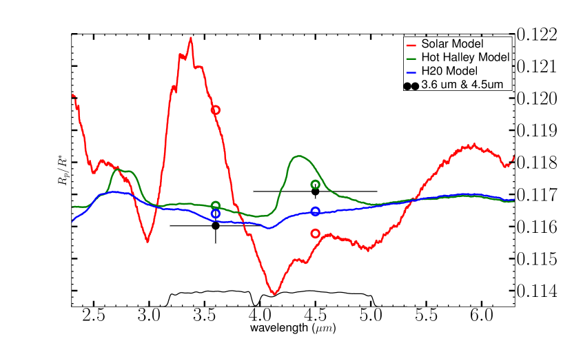
Figure 12: Comparison between our Spitzer results and three recent models for the atmosphere of GJ1214b, from Benneke & Seager (2012): a cloudless solar model, a comet-like model, and a water vapor model.

Prior to an exhaustive analysis of all data versus all models, we mention what our new Spitzer data alone immediately reveal and/or constrain concerning the atmosphere of GJ1214b. We (BB & SS) generated three new model atmospheres for GJ1214b at an equilibrium temperature of 546 K, based on the methodology of Benneke & Seager (2012). The models are: 1) a H-rich solar abundance model, 2) a ‘Hot-Halley’ composition model which begins with solar composition and adds minor molecular constituents from accreted icy material (Benneke & Seager, 2012), and 3) a pure water vapor atmosphere. Figure 12 shows the result of integrating these three models over the Spitzer observational bandpasses, and including the stellar intensity using a PHOENIX model having Teff/log(g)/[M/H] = 3000 K/5.0/0.3. Based on this comparison, the solar composition model is eliminated based on the Spitzer data alone. The water vapor model is preferred over the hot Halley model, based on the $\chi^{2}$ analysis described below. Moreover, we expect that methane-rich models having large scale heights (not illustrated) will be rejected by the Spitzer data, due to the relative lack of an enhanced radius in the 3.6 $\mu$m band - that contains the strong $\nu_{3}$ band of methane.

6.3 A $\chi^{2}$ Analysis

To gain further quantitative insight, we weighted the three models from Benneke & Seager (2012) discussed above, as well as all of the models given by Howe & Burrows (2012) over the observed bandpasses of all extant transit observations of GJ1214, including the TRAPPIST and warm Spitzer data reported here. We fit the models to the data using a $\chi^{2}$ analysis, as described below. Berta et al. (2012) applied a similar $\chi^{2}$ analysis to data from Hubble/WFC3, but not to the complete set of data that we do here, and in particular not including our new and precise results in the warm Spitzer bands. The utility of $\chi^{2}$ is well known to be problematic when combining data from different observational groups. However, $\chi^{2}$ is at least an objective way to compare different models, and we explicitly consider one cause of observer-to-observer systematic differences in Sec. 6.4.

To evaluate and compare possible models of the planetary atmosphere, we fit each model to the data by adding an adjustable constant (i.e., wavelength-independent offset) to the modeled values of $R_{p}/R_{*}$. We choose the constant to minimize the $\chi^{2}$ of the difference between the adjusted model and the data. Adding this constant is equivalent to increasing (or decreasing) the size of the opaque (i.e., solid) portion of the planet by a small amount. That effectively varies the surface gravity of the planet, and would strictly speaking be inconsistent with the model that is being adjusted. However, the planetary radius at a given atmospheric pressure level is not known at a level of accuracy comparable to the adjustments we are making. Moreover, the requisite adjustments in the model output (typically, $0.0005$ in $R_{p}/R_{*}$), correspond to less than 1% differences in surface gravity. We therefore find this procedure to be a valid and useful tool for testing models versus the observations, and we note that a similar procedure was used by Berta et al. (2012). We fit the three models shown in Figure 12 (Benneke & Seager, 2012), together with all of the models from Howe & Burrows (2012), and we calculate $\chi^{2}$ values for each fit. We also fit a flat line to the data, i.e., a planetary radius that does not vary with wavelength - indicating no signature of the atmosphere.

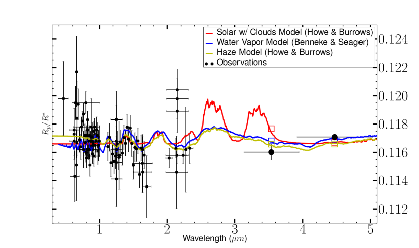
Figure 13: Comparison between all published observations of GJ1214b, including our Spitzer and TRAPPIST transits, and recent models. Three models having the lowest $\chi^{2}$ are illustrated: a water vapor model from Benneke & Seager (2012) (blue curve), a solar abundance model with very high cloud tops (at 0.1 mbars, red curve), and a model with 1-percent water vapor, and a thick tholin haze of 0.1 $\mu$m particles extending to very high altitude (1 $\mu$bar, yellow curve). The latter two models are from Howe & Burrows (2012).

Several of the best fitting models are shown in Figure 13, compared to the entirety of published radii for this planet. In total, there are 97 observations of $R_{p}/R_{*}$ versus wavelength on Figure 13. The water atmosphere from Figure 12, and two models from Howe & Burrows (2012), are also included on Figure 13. For the Figure, the models are overplotted monochromatically, without integrating over the bandpass. However, the $\chi^{2}$ values are calculated by integrating the model over the bandpass of each observation as described above, and adopting the observed errors from each source. In the case of multi-band analyses (Kundurthy et al., 2011), we use the total bandpass from multiple filters. For the three overplotted models we also show the values for the integrals over the Spitzer bandpasses, as open symbols.

With 96 degrees of freedom, models can only be rejected at the 99.9% confidence level if they have a $\chi^{2}$ exceeding 144.6. Among the possible models, The pure water atmosphere from Benneke & Seager (2012) yields $\chi^{2}=142.7$ for 96 degrees of freedom. The hot Halley and solar composition models from Benneke & Seager (2012) have $\chi^{2}$ values of 167.9 and 1054.7 respectively, and are unlikely descriptions of GJ1214b’s atmosphere. The solar composition model in particular is strongly rejected unless high clouds are included (see below). In this respect, we note that some discussion of a solar composition atmosphere has occurred with respect to transit observations near 2 $\mu$m (Croll et al., 2011; Bean et al., 2011). We here emphasize that a cloudless solar composition model is incompatible with the Spitzer data alone, as well as with the totality of the observations over all wavelengths. The issue of the transit depth near 2 $\mu$m - while an important datum - is not crucial to rejecting a solar composition atmosphere.

Our improvement in the observed Spitzer precision at 3.6 $\mu$m - overlapping the strong $\nu_{3}$ band of methane, prompts us to investigate the methane-composition models of Howe & Burrows (2012). All of their methane compositions have $\chi^{2}$ above 184.6 (the value for 1% methane). However, a solar composition model having high clouds (down to pressures of 0.1 mbars) produces an acceptable $\chi^{2}=145.5$. This model is plotted as the red line on Figure 13; it predicts an increase in radius in the difficult-to-observe regions near 2.7 and 3.3 $\mu$m. The best fit to the data is the yellow line on Figure 13, having $\chi^{2}=119.8$. This model, from Howe & Burrows (2012), contains a dense haze of small (0.1 $\mu$m) tholin particles, extending to very high altitudes (1 $\mu$bar). It was disfavored by Howe & Burrows (2012), but our methodology is different in that we incorporate a marginally additive constant when fitting the models. However, we point out that also among the acceptable models is a flat line (not illustrated on Figure 13). This null hypothesis (no atmosphere detected) yields $\chi^{2}=137.0$.

6.4 Systematic Differences Between Observers

One further check on the acceptable models is to focus on the difference between our precise Spitzer radii and very precise radii derived at other wavelengths, i.e., by Bean et al. (2011) and Berta et al. (2012). As noted at the end of Sec. 4.5, we fix the variable orbital parameters ($a/R_{*}$ and $i$) at the values derived by Bean et al. (2011) and Berta et al. (2012) and derive a lower value of $R_{p}/R_{*}$ at 4.5 $\mu$m by about 0.001 (Table 5). Using that alternative value in our $\chi^{2}$ analysis is one way of evaluating the possible effect of observer-to-observer differences in radii. This procedure increases the $\chi^{2}$ values of most models, but by varying amounts. Interestingly, the two least affected models are the flat line, whose $\chi^{2}$ increases by $\delta\chi^{2}=+1.6$, and the tholin-haze model. The water model from Benneke & Seager (2012) has $\delta\chi^{2}=+8.4$, and their hot Halley model has $\delta\chi^{2}=+19.8$. The scattering tholin-haze model from Howe & Burrows (2012) remains as the lowest absolute $\chi^{2}$, and has $\delta\chi^{2}=-2.3$, i.e. it becomes more likely, not less likely. We conclude that, even when systematic differences among observational groups are considered, a scattering atmosphere is currently the best estimate for GJ1214b. However, we are unable to explore the vast phase space of other possible sources of systematic error. Hence we also conclude that the null hypothesis (no atmosphere detected) remains among the most favored models, especially when systematic errors are considered.

6.5 Summary of Implications for the Atmosphere of GJ1214b

We have obtained new radii for GJ1214b in the I+z band using TRAPPIST, and very precise radii at 3.6- and 4.5 $\mu$m using Warm Spitzer in a long series of new observations. Our $\chi^{2}$ analysis indicates that the best-fit model for the atmosphere of GJ1214b contains a haze of small particles extending to high altitudes, although pure water vapor models remain a possibility. However, a flat line is among the best-fitting models, particularly when observer-to-observer systematic differences are considered. Therefore we extend the conclusion of Berta et al. (2012) concerning the flatness of the transmisison spectrum from 1.1- to 1.7 $\mu$m to include our new high-precision Spitzer measurements at 3.6- and 4.5 $\mu$m. The atmosphere of GJ1214b is not unequivocally detected at this point in time.


This work is based on observations made with the Spitzer Space Telescope, which is operated by the Jet Propulsion Laboratory, California Institute of Technology under a contract with NASA. Support for this work was provided by NASA through an award issued by JPL/Caltech. We thank the Spitzer staff for their hard work and dedication in implementing these difficult observations, and the anonymous referee for a careful review of this paper.

Table 1: Results of fitting to 13 individual transits of GJ1214b at 4.5 $\mu$m, plus the transit observed by Désert et al. (2011).

Epoch	$T_{c}-2450000(BJD_{TDB})$	$i$	$a/{R_{*}}$	${R_{p}}/{R_{*}}$	$c_{0}$
211	$5314.214114\pm 0.000085$	$88.81\pm 0.39$	$14.92\pm 0.40$	$0.11726\pm 0.00105$	$0.133\pm 0.074$
443	$5680.867846\pm 0.000059$	$89.30\pm 0.33$	$15.51\pm 0.28$	$0.11735\pm 0.00064$	$0.097\pm 0.046$
444	$5682.448272\pm 0.000067$	$88.89\pm 0.37$	$14.98\pm 0.39$	$0.11692\pm 0.00077$	$0.208\pm 0.047$
445	$5684.028698\pm 0.000056$	$89.88\pm 0.36$	$15.72\pm 0.27$	$0.11681\pm 0.00057$	$0.126\pm 0.041$
446	$5685.609139\pm 0.000048$	$89.11\pm 0.23$	$15.24\pm 0.24$	$0.11625\pm 0.00034$	$0.118\pm 0.029$
447	$5687.189632\pm 0.000065$	$88.23\pm 0.26$	$14.11\pm 0.41$	$0.11796\pm 0.00054$	$0.059\pm 0.051$
448	$5688.769880\pm 0.000094$	$89.42\pm 0.36$	$15.38\pm 0.30$	$0.11586\pm 0.00100$	$0.170\pm 0.067$
449	$5690.350385\pm 0.000052$	$88.34\pm 0.23$	$14.33\pm 0.36$	$0.11803\pm 0.00052$	$0.098\pm 0.050$
450	$5691.930794\pm 0.000067$	$88.22\pm 0.25$	$14.24\pm 0.43$	$0.11865\pm 0.00049$	$0.033\pm 0.033$
451	$5693.511181\pm 0.000058$	$88.81\pm 0.25$	$14.95\pm 0.29$	$0.11737\pm 0.00053$	$0.130\pm 0.046$
453	$5696.671937\pm 0.000073$	$88.68\pm 0.37$	$14.75\pm 0.41$	$0.11606\pm 0.00075$	$0.189\pm 0.047$
454	$5698.252258\pm 0.000047$	$88.93\pm 0.28$	$15.14\pm 0.30$	$0.11567\pm 0.00047$	$0.056\pm 0.029$
455	$5699.832550\pm 0.000068$	$88.24\pm 0.28$	$14.17\pm 0.43$	$0.11802\pm 0.00062$	$0.070\pm 0.058$
456	$5701.413161\pm 0.000059$	$89.61\pm 0.30$	$15.41\pm 0.23$	$0.11549\pm 0.00066$	$0.205\pm 0.042$

Table 2: Results of fitting to two individual transits of GJ1214b at 3.6 $\mu$m, plus the transit observed by Désert et al. (2011).

Epoch	$T_{c}-2450000(BJD_{TDB})$	$i$	$a/{R_{*}}$	${R_{p}}/{R_{*}}$	$c_{0}$
210	$5312.633724\pm 0.000072$	$89.998\pm 0.324$	$15.659\pm 0.160$	$0.11665\pm 0.00082$	$0.200\pm 0.061$
564	$5872.096721\pm 0.000094$	$89.144\pm 0.383$	$15.331\pm 0.354$	$0.11619\pm 0.00121$	$0.114\pm 0.065$
565	$5873.677187\pm 0.000062$	$89.221\pm 0.296$	$15.418\pm 0.281$	$0.11584\pm 0.00066$	$0.135\pm 0.049$

Table 3: Results of fitting to 7 individual transits of GJ1214b in the I+z-band, observed by TRAPPIST (Gillon et al., 2012).

Epoch	$T_{c}-2450000(BJD_{TDB})$	$i$	$a/{R_{*}}$	${R_{p}}/{R_{*}}$	$c_{0}$	$c_{1}$
412	$5631.875656\pm 0.000092$	$88.035\pm 0.365$	$13.743\pm 0.443$	$0.11680\pm 0.00135$	$0.237\pm 0.094$	$0.073\pm 0.177$
424	$5650.840034\pm 0.000152$	$87.805\pm 0.384$	$13.215\pm 0.515$	$0.12389\pm 0.00216$	$0.331\pm 0.176$	$0.110\pm 0.220$
436	$5669.805222\pm 0.000110$	$88.990\pm 0.436$	$14.945\pm 0.562$	$0.11389\pm 0.00275$	$0.422\pm 0.170$	$0.267\pm 0.345$
441	$5677.706878\pm 0.000170$	$88.965\pm 0.412$	$14.923\pm 0.550$	$0.11573\pm 0.00331$	$0.428\pm 0.198$	$0.008\pm 0.370$
443	$5680.867699\pm 0.000131$	$88.336\pm 0.397$	$14.049\pm 0.486$	$0.12138\pm 0.00182$	$0.012\pm 0.153$	$0.602\pm 0.298$
453	$5696.672075\pm 0.000135$	$89.873\pm 0.671$	$14.932\pm 0.741$	$0.10802\pm 0.00296$	$0.646\pm 0.142$	$0.141\pm 0.242$
455	$5699.832535\pm 0.000143$	$88.360\pm 0.460$	$14.516\pm 0.641$	$0.11877\pm 0.00228$	$0.343\pm 0.138$	$0.005\pm 0.268$

Table 4: Results of fitting to composite transits, i.e.: simultaneous fits, averaging individual transits, and fitting to phased & binned transits.

Method / Channel	$T_{c}-2450000(BJD_{TDB})$	$i$	$a/{R_{*}}$	${R_{p}}/{R_{*}}$	$c_{0}$	$c_{1}$
Simultaneous 3.6 $\mu$m	$4966.524895\pm 0.000047$	$89.566\pm 0.139$	$15.607\pm 0.104$	$0.11607\pm 0.00030$	$0.156\pm 0.022$	fixed at 0.0
Simultaneous 4.5 $\mu$m	$4966.524918\pm 0.000030$	$88.794\pm 0.061$	$15.049\pm 0.095$	$0.11710\pm 0.00017$	$0.110\pm 0.014$	fixed at 0.0
Simultaneous TRAPPIST I+z	$4966.524881\pm 0.000063$	$88.240\pm 0.230$	$14.011\pm 0.288$	$0.11873\pm 0.00111$	$0.320\pm 0.097$	$0.187\pm 0.176$
Averaged individual 3.6 $\mu$m	$4966.524898\pm 0.000076$	$89.469\pm 0.221$	$15.564\pm 0.080$	$0.11616\pm 0.00019$	$0.148\pm 0.021$	fixed at 0.0
Averaged individual 4.5 $\mu$m	$4966.524925\pm 0.000027$	$88.803\pm 0.127$	$15.090\pm 0.137$	$0.11699\pm 0.00026$	$0.110\pm 0.015$	fixed at 0.0
Averaged individual TRAPPIST I+z	$4966.524968\pm 0.000077$	$88.437\pm 0.057$	$14.207\pm 0.239$	$0.11793\pm 0.00182$	$0.324\pm 0.068$	$0.146\pm 0.073$
Phased & binned 3.6 $\mu$m	$4966.524156\pm 0.000043$	$89.469\pm 0.143$	$15.547\pm 0.091$	$0.11602\pm 0.00055$	$0.158\pm 0.035$	fixed at 0.0
Phased & binned 4.5 $\mu$m	$4966.524297\pm 0.000016$	$88.439\pm 0.061$	$14.442\pm 0.093$	$0.11709\pm 0.00022$	$0.128\pm 0.018$	fixed at 0.0
Phased & binned TRAPPIST I+z	$4966.524122\pm 0.000079$	$88.314\pm 0.177$	$14.053\pm 0.259$	$0.11803\pm 0.00079$	$0.263\pm 0.107$	$0.316\pm 0.149$

Table 5: Summary of results for $R_{p}/R_{*}$ derived at different wavelengths using different methods. The phased & binned transit results for $R_{p}/R_{*}$ are given for several cases: our best-fit orbital parameters ($a/R_{*}$, $i$), as well as $R_{p}/R_{*}$ when we force the orbital parameters to have the values determined by Bean et al. (2011) (14.97, 88.94) and Berta et al. (2012) (15.31, 89.30), respectively.

Method	${R_{p}}/{R_{*}}$
Spitzer 4.5 $\mu$m
Simultaneous	$0.1171\pm 0.0002$
Averaged Individual	$0.1170\pm 0.0003$
Phased & binned Best-fit orbital	$0.1171\pm 0.0002$
Bean orbital	$0.1161\pm 0.0003$
Berta orbital	$0.1160\pm 0.0003$
Spitzer 3.6 $\mu$m
Simultaneous	$0.1161\pm 0.0003$
Averaged Individual	$0.1162\pm 0.0001$
Phased & binned
Best-fit orbital	$0.1160\pm 0.0006$
Bean orbital	$0.1163\pm 0.0002$
Berta orbital	$0.1161\pm 0.0002$
TRAPPIST I+z band
Simultaneous	$0.1187\pm 0.0011$
Averaged Individual	$0.1179\pm 0.0018$
Phased & binned
Best-fit orbital	$0.1180\pm 0.0005$
Bean orbital	$0.1177\pm 0.0005$
Berta orbital	$0.1172\pm 0.0005$

References

- Agol et al. (2010) Agol, E., Cowan, N. B., Knutson, H. A., Deming, D., Steffen, J. H., Henry, G. W., & Charbonneau, D., 2010, ApJ, 721, 1861.
- Allard & Hauschildt (1995) Allard, F., & Hauschildt, P. H., 1995, ApJ, 445, 433.
- Ballard et al. (2010) Ballard, S., Charbonneau, D., Deming, D., Knutson, H. A., Christiansen, J. L., Holman, M. J., Fabrycky, D., Seager, S., & A’Hearn, M. F., 2010, PASP, 122, 1341.
- Bean et al. (2010) Bean, J. L., Miller-Ricci Kempton, E., & Homeier, D., 2010, Nature, 468, 669.
- Bean et al. (2011) Bean, J. L., and 9 co-authors, 2011, ApJ, 743, id.92.
- Benneke & Seager (2012) Benneke, B., & Seager, S., 2012, submitted to ApJ, astro-ph/1203.4018.
- Berta et al. (2011) Berta, Z. K., Charbonneau, D., Bean, J., Irwin, J., Burke, C. J., Dësert, J.-M., Nutzman, P. & Falco, E. E., 2011, ApJ, 736, id.12.
- Berta et al. (2012) Berta, Z. K., & 9 co-authors, 2012, ApJ, 747, id.35.
- Carter et al. (2011) Carter, J. A., Winn, J. N., Holman, M. J., Fabrycky, D., Berta, Z. K., Burke, C. J., & Nutzman, P., 2011, ApJ, 730, id.82.
- Charbonneau et al. (2009) Charbonneau, D., and 18 co-authors, 2009, Nature, 462, 891.
- Claret & Bloemen (2011) Claret, A., & Bloemen, S., 2011, A&A, 529, id.A75
- Croll et al. (2011) Croll, B., Albert, L., Jayawardhana, R., Miller-Ricci Kempton, E., Fortney, J. J., Murray, N., & Neilson, Hilding, 2011, ApJ, 736, id.78.
- Crossfield et al. (2011) Crossfield, I. J. M., Barman, T., & Hansen, B. M. S., 2011, ApJ, 736, id.132.
- Deming et al. (2009) Deming, D., and 11 co-authors, 2009, PASP, 121, 883.
- Deming et al. (2011) Deming, D., Sada, P. V., Jackson, B., Peterson, S. W., Agol ,E., Knutson, H. A., Jennings, D. E., Haase, F., & Bays, K., 2011, ApJ, 740, id.33.
- Désert et al. (2011) Dësert, J. M., Bean, J., Miller-Ricci Kempton, E., Berta, Z. K., Charbonneau, D., Irwin, J., Fortney, J. J., Burke, C. J., & Nutzman, P., 2011, ApJ, 731, id.L40.
- Désert et al. (2011b) Dësert, J. M., Sing, D., Vidal-Madjar, A., Hebrard, G., Ehrenreich, D., Lecavelier Des Estangs, A., Parmentier, V., Ferlet, R., & Henry, G. W., 2011, A&A, 526, id.A12.
- Ford (2005) Ford, E. B., 2005, AJ, 129, 1706.
- Gillon et al. (2007) Gillon, M., Demory, B.-O., Barman, T., Bonfils, X., Mazeh, T., Pont, F., Udry, S., Mayor, M., & Queloz, D., 2007, A&A, 471, L51.
- Gillon et al. (2011) Gillon, M., Jehin E., Magain, P., Chantry, V., Hutsemekers, D., Manfroid, J., Queloz, D., & Udry, S., 2011, in ‘Detection and Dynamics of Transiting Exoplanets,’ EPJ Web of Conferences, eds. F. Bouchy, R. Diaz, & C. Moutou, Vol. 11, id.06002.
- Gillon et al. (2012) Gillon, M., Demory, B.-O., Deming, D., Seager, S., et al., 2012, in preparation for A&A.
- Howe & Burrows (2012) Howe, A. R., & Burrows, A. S., 2012, ApJ, 756, 176.
- Jehin et al. (2011) Jehin, E., Gillon, M., Queloz, D., et al., The Messenger, 145, 2.
- Knutson et al. (2012) Knutson, H. A., & 13 co-authors, 2012, ApJ, 754, 22.
- Kundurthy et al. (2011) Kundurthy, P., Agol, E., Becker, A. C., Barnes, R., Williams, B., & Mukadam, A., 2011, ApJ, 731, 123.
- Lewis et al. (2013) Lewis, N. K., & 23 co-authors, 2013, submitted to ApJ.
- Liddle (2007) Liddle, A. R., 2007, MNRAS, 377, L74.
- Mandel & Agol (2002) Mandel, K., & Agol, E., 2002, ApJ, 580, L171.
- Mighell (2005) Mighell, K. J., 2005, MNRAS, 361, 861.
- Miller-Ricci & Fortney (2010) Miller-Ricci Kempton, E., & Fortney, J. J., 2010, ApJ, 716, L74.
- Murgas et al. (2012) Murgas, F., Pallé, E., Cabrera-Lawers, A., Colón, K.D., Martín, E.L., Parviainen, H., 2012, A&A, 554, id.A41.
- Narita et al. (2012) Narita, N., Nagayama, T., Suenaga, T., Fukui, A., Ikoma, M., Nakajima, Y., Nishiyama, S., Tamura, M., submitted to PASJ, astro-ph/1210.3169.
- Nutzman & Charbonneau (2008) Nutzman, P., & Charbonneau, D., 2008, PASP, 120, 317.
- de Mooij et al. (2012) de Mooij, E. J. W., and 10 co-authors, 2012, A&A, 538, id.A46.
- Rice & Strassmeier (1998) Rice, J. B., Strassmeier, K. G., 1998, A&A, 336, 972.
- Rogers & Seager (2010) Rogers, L., & Seager, S., 2010, ApJ, 716, 1208.
- Sada et al. (2010) Sada, P. V., Deming, D., Jackson, B., Jennings, D. E., Peterson, S. W., Haase, F., Bays, K., O’Gorman, E., & Lundsford, A., 2010, ApJ, 720, L215.
- Sing et al. (2009) Sing, D., Dësert, J.-M., Des Estangs, L., Ballester, G. E., Vidal-Madjar, A., Parmentier, V., Hebrard, G., & Henry, G. W., 2009, A&A, 505, 891.
- Stevenson et al. (2010) Stevenson, K. B., & 9 co-authors, 2010, Nature, 464, 1161.