Habitable Zones Around Main-Sequence Stars: New Estimates

Abstract

Identifying terrestrial planets in the habitable zones (HZs) of other stars is one of the primary goals of ongoing radial velocity and transit exoplanet surveys and proposed future space missions. Most current estimates of the boundaries of the HZ are based on 1-D, cloud-free, climate model calculations by Kasting et al. (1993). However, this model used band models which were based on older HITRAN and HITEMP line-by-line databases. The inner edge of the HZ in Kasting et al. (1993) model was determined by loss of water, and the outer edge was determined by the maximum greenhouse provided by a $\rm{CO_{2}}$ atmosphere. A conservative estimate for the width of the HZ from this model in our Solar system is 0.95-1.67 AU.

Here, an updated 1-D radiative-convective, cloud-free climate model is used to obtain new estimates for HZ widths around F, G, K and M stars. New $\rm{H_{2}O}$ and $\rm{CO_{2}}$ absorption coefficients, derived from the HITRAN 2008 and HITEMP 2010 line-by-line databases, are important improvements to the climate model. According to the new model, the water loss (inner HZ) and maximum greenhouse (outer HZ) limits for our Solar System are at $0.99$ AU and $1.70$ AU, respectively, suggesting that the present Earth lies near the inner edge. Additional calculations are performed for stars with effective temperatures between $2600$ K and $7200$ K, and the results are presented in parametric form, making them easy to apply to actual stars. The new model indicates that, near the inner edge of the HZ, there is no clear distinction between runaway greenhouse and water loss limits for stars with T${}_{eff}\lesssim 5000$ K which has implications for ongoing planet searches around K and M stars. To assess the potential habitability of extrasolar terrestrial planets, we propose using stellar flux incident on a planet rather than equilibrium temperature. This removes the dependence on planetary (Bond) albedo, which varies depending upon the host star’s spectral type. We suggest that conservative estimates of the HZ (water loss and maximum greenhouse limits) should be used for current RV surveys and Kepler mission to obtain a lower limit on $\eta_{\oplus}$, so that future flagship missions like TPF-C and Darwin are not undersized. Our model does not include the radiative effects of clouds; thus, the actual HZ boundaries may extend further in both directions than the estimates just given.

1 Introduction

As of November, 2012, more than 800 extra-solar planetary systems have been detected, and $>2000$ additional candidate systems from the Kepler mission are waiting to be confirmed (Batalha et al., 2012). One of the primary goals of the ongoing radial velocity (RV) and transit surveys is to identify a terrestrial mass planet ($0.3-10$M_⊕) in the so-called Habitable Zone (HZ), which is traditionally defined as the circumstellar region in which a terrestrial-mass planet with a $\rm{CO_{2}}$-$\rm{H_{2}O}$-N₂ atmosphere can sustain liquid water on its surface (Huang, 1959; Hart, 1978; Kasting et al., 1993; Underwood et al., 2003; Selsis et al., 2007b; Kaltenegger et al., 2011b; Pierrehumbert & Gaidos, 2011). Several potential HZ planet candidates have already been detected, (Udry et al., 2007; Pepe et al., 2011a; Borucki et al., 2011; Bonfils et al., 2011; Borucki et al., 2012; Vogt et al., 2012; Tuomi et al., 2012a, b) and it is expected that this number will greatly increase as time passes (Batalha et al., 2012). In the near future we may be able to study habitable planets orbiting nearby M stars. These planets are relatively close to their parent stars, leading to shorter orbital periods and an increase in the probability of a transit. NASA’s James Webb Space Telescope (JWST), scheduled to launch in 2018, is considered to be marginally capable of obtaining a transit spectrum of an Earth-like planet orbiting a late M dwarf (Clampin et al., 2007; Kaltengger & Traub, 2009; Deming et al., 2009). Several other surveys are either underway (Nutzman & Charbonneau, 2008, MEARTH) or getting ready to be commissioned (Mahadevan et al., 2012, HPF) in an attempt to discover rocky planets in the HZs of low mass stars.

The HZ limits that were cited in many recent discoveries were obtained from 1-D radiative-convective, cloud-free climate model calculations by Kasting et al. (1993). For our Sun, these authors estimated the boundaries of the HZ to be $0.95$ AU for the inner edge and $1.67$ AU for the outer edge. These values represent the “water loss” and “maximum greenhouse” limits, respectively. Other, less conservative limits for the inner edge are the “runaway greenhouse” and “recent Venus” limits. The latter estimate is empirical, based on the inference that Venus has not had liquid water on its surface for at least the last 1 billion years (Solomon & Head, 1991). For the outer edge, there is a corresponding “early Mars” empirical estimate, based on the inference that Mars did have liquid water on its surface 3.8 billion years ago. (The “1st $\rm{CO_{2}}$ condensation” limit of Kasting et al. (1993), should now be disregarded, as it has been shown that $\rm{CO_{2}}$ clouds generally warm a planet’s climate (Forget & Pierrehumbert, 1997)). Some studies have investigated the effects of clouds on planetary emission spectra of Earth-like planets in a 1D model (Kitzmann et al., 2011a, b), while others studied the habitability of specific systems, particularly Gl 581, in 1D (Wordsworth et al., 2010; Von Paris et al., 2011a; Kaltenegger et al., 2011a) and 3D (Wordsworth et al., 2011; Pierrehumbert, 2011). Several other studies (Underwood et al., 2003; Selsis et al., 2007b) parameterized these results to estimate relationships between HZ boundaries and stellar parameters for stars of different spectral types.

Although these studies provided useful estimates of the HZ width, the Kasting et al. (1993) model has become outdated, for several reasons:

1. Kasting et al. (1993) used ‘band models’ for $\rm{H_{2}O}$ and $\rm{CO_{2}}$ absorption in the thermal-infrared. These coefficients were considered valid up to $\sim 700$ K. These coefficients were later replaced (Mischna et al., 2000) by coefficients generated using the correlated-k technique (Mlawer et al., 1997; Kato et al., 1999). A line-by-line (LBL) radiative transfer model, in this case LBLRTM (Clough & Iocono, 1995), was used to generate detailed spectra for $\rm{H_{2}O}$ and $\rm{CO_{2}}$ at a variety of different temperatures and pressures. Once the detailed spectra were calculated, separate broad-band k-coefficients for both $\rm{H_{2}O}$ and $\rm{CO_{2}}$ were generated by R. Freedman using standard procedures. But these coefficients were only derived for temperatures $<350$ K and should therefore underestimate thermal-IR absorption in warm, moist greenhouse atmospheres. (This prediction was verified by direct experimentation with that model.) Furthermore, the coefficients adopted by Mischna et al. (2000) and used in subsequent climate modeling studies by the Kasting research group were obtained using HITRAN 1996 database and had not been updated since then.

2. Recent studies (Halevy et al., 2009; Wordsworth et al., 2010) have pointed that the Kasting et al. (1993) model may have significantly overestimated absorption of thermal-IR radiation by collision-induced absorption (CIA) bands of $\rm{CO_{2}}$, which may affect the outer edge of the HZ.

3. The Kasting et al. (1993) calculations spanned stellar effective temperatures from $7200$ K to $3700$ K, corresponding approximately to stellar classes F0 to M0. Stellar effective temperature affects the HZ boundaries because the radiation from F stars is bluer relative to that from the Sun, whereas the radiation from K and M stars is redder, and this affects calculated planetary albedos. The HZ limits from Kasting et al. (1993) model do not include M stars with effective temperatures lower than $3700$ K. As pointed out above, such stars are promising candidates for current observational surveys because their HZs are closer to the star. Therefore, potential rocky planets in the HZs will have shorter orbital periods and higher probability of transit.

In this paper we address all the above major issues with the goal of deriving new, improved estimates for the boundaries of the HZ. The outline of the paper is as follows: In §2 we describe our 1-D cloud-free climate model, corresponding model updates and model validation with other studies. In §3 we present results from our climate model and discuss various HZ limits for our Earth. §4 presents HZ boundaries around F, G, K and M spectral stellar spectral types, then provides a generalized expression to calculate HZ boundaries and compares these boundaries with previous studies. We discuss the implications of these new results for currently known exoplanet planetary systems in §5 and present our conclusions in §6.

2 Model description

We used a one-dimensional, radiative-convective, cloud-free climate model based on Kasting (1988) for the inner edge of the HZ (IHZ) and Kasting (1991) for the outer edge of the HZ (OHZ) calculations. Following Kasting et al. (1993), we assumed an Earth-mass planet with an $\rm{H_{2}O}$ (IHZ) or $\rm{CO_{2}}$ (OHZ) dominated atmosphere for our base model. Sensitivity studies for different planetary masses are described in the following section. Both the inner and outer edge calculations relied on so-called “inverse climate modeling”, in which the surface temperature is specified, and the model is used to calculate the corresponding solar flux needed to sustain it. To do this, the atmosphere was divided into $101$ layers, and a specific pressure-temperature profile was assumed. For the inner edge, this consisted of a moist pseudoadiabat extending from the surface up to an isothermal (200 K) stratosphere. Methodology for calculating the pseudoadiabat was taken from Appendix A of Kasting (1988). The surface temperature was varied from 200-2200 K during the course of the calculations. For the outer edge, the surface temperature was fixed at 273 K, and the $\rm{CO_{2}}$ partial pressure was varied from 1 to 37.8 bar (the saturation $\rm{CO_{2}}$ partial pressure at that temperature). A moist $\rm{H_{2}O}$ adiabat was assumed in the lower troposphere, and a moist $\rm{CO_{2}}$ adiabat was used in the upper troposphere when condensation was encountered, following the methodology in Appendix B of Kasting (1991).

$\rm{H_{2}O}$ and $\rm{CO_{2}}$ clouds are neglected in the model, but the effect of the former is accounted for by increasing the surface albedo, as done in previous climate simulations by the Kasting research group (Kasting, 1991; Haqq-Misra et al., 2008). It has been argued that this methodology tends to overestimate the greenhouse effect of dense $\rm{CO_{2}}$ atmospheres (Goldblatt & Zahnle, 2011). By contrast, our neglect of $\rm{CO_{2}}$ clouds may cause us to underestimate the greenhouse effect of such atmospheres (Forget & Pierrehumbert, 1997). Realistically determining the effects of clouds would require a 3-D climate model, as most clouds form in updrafts, which are absent in 1-D models. Some 1-D climate modeling studies include partial cloud coverage (Selsis et al., 2007b) and/or parameterized microphysical cloud model (Colaprete & Toon, 2003; Zsom et al., 2012), but we do not consider them here because we can not model them self-consistently in our model. The effects of clouds on the inner and outer edge boundaries are qualitatively understood, as discussed later in the paper. Testing these predictions quantitatively using 3-D climate models should be a fruitful topic for future research.

Radiative transfer was handled by methods used in recent versions of the Kasting group climate model but with updated absorption coefficients (see next section). A $\delta$ two-stream approximation (Toon et al., 1989) was used to calculate the net absorbed solar radiation for each of the $101$ layers, using separate eight-term, correlated-$k$ coefficients for both $\rm{CO_{2}}$ and $\rm{H_{2}O}$ to parameterize absorption in each of the $38$ solar spectral intervals ranging from $0.2-4.5\mu$m. These terms are convolved with each other in each spectral interval, resulting in 64 separate radiative transfer calculations per interval. The solar flux was averaged over six zenith angles (11.0^∘, 25.3^∘, 39.6^∘, 54^∘, 68.4^∘, 82.8^∘) using Gaussian quadrature. The net outgoing infrared radiation per layer was calculated using separate eight-term correlated-$k$ coefficients for $\rm{H_{2}O}$ and $\rm{CO_{2}}$ in $55$ spectral intervals extending from $0-15,000$ cm^-1. We used double gauss quadrature in place of a standard gaussian scheme (Sykes, 1952; Thomas & Stamnes, 2002) using a code written by Ramirez. Half of the k-coefficients are chosen within the g-space interval 0.95-1.00 for improved resolution of the steeply rising portion of the cumulative distribution function, yielding smoother stratospheric temperature behavior.

These coefficients also needed to be convolved with each other, as in the solar calculation. This produces 8$\times$ 8 $\times$ 55 $=$ 3520 separate thermal-IR radiative transfer calculations at each time step in the climate model. This number is multiplied by a factor of 6 when we include $\rm{CH_{4}}$ in the model, using 6-term sums, and by another factor of 6 when we include C₂H₆. Thus, from a practical standpoint, the utility of this approach diminishes as the number of included greenhouse gases increases.

2.1 Model Updates

The following are the most significant updates to the climate model:

1. We have derived new k- coefficients using a tool called KSPECTRUM. It is a program to produce high-resolution spectrum of any gas mixture, in any thermodynamical conditions, from line-by-line (LBL) databases such as HITRAN 2008 (Rothman et al., 2009) and HITEMP 2010 (Rothman et al., 2010). It is intended to produce reliable spectra, which can then be used to compute k-distribution data sets that may be used for subsequent radiative transfer analysis. The source code and a detailed description of the program is available at http://code.google.com/p/kspectrum/.

   We have produced two sets of coefficients, one using HITRAN 2008 and another using the HITEMP 2010 database. For the HITRAN database we generated a matrix of 8-term absorption coefficients for both $\rm{H_{2}O}$ and $\rm{CO_{2}}$, using KSPECTRUM, for the following range of pressures and temperatures: $p(bar)=[10^{-5},10^{-4},10^{-3},10^{-2},10^{-1},1,10,10^{2}]$ and $T(K)=[100,150,200,250,300,350,400,600]$. In the case of HITEMP, 8-term absorption coefficients were derived only for $\rm{H_{2}O}$, as our IHZ is $\rm{H_{2}O}$-dominated at high temperatures ($\geq 300$ K) with only trace amounts of $\rm{CO_{2}}$ (330 parts per million). The following grid was used to derive the $\rm{H_{2}O}$ HITEMP coefficients: $p(bar)=[10^{-1},1,10,10^{2}]$ and $T(K)=[350,400,600]$. The grid is condensed because of the high number of line transitions in the HITEMP database compared to HITRAN. The computational resources needed to derive absorption coefficients for the entire range of pressure & temperatures would be prohibitively large. Moreover, as discussed further below, we justify the selection of this condensed grid by showing that the differences in coefficients generated from HITRAN and HITEMP become negligible below 350 K.

   In generating the $k-$coefficients, we have used different methodologies for $\rm{CO_{2}}$ and $\rm{H_{2}O}$. For CO2, we truncated the spectral lines at $500$ cm^-1 from the line center. Experimental evidence indicates that the absorption by $\rm{CO_{2}}$ is overestimated if Lorentzian line shapes are used (Burch et al., 1969; Fukabori et al., 1986; Bezard et al., 1990; Halevy et al., 2009). Therefore, we used the prescription of Perrin & Hartmann (1989) for ‘sub-Lorentzian’ absorption in the far wings of the lines when running KSPECTRUM. For $\rm{H_{2}O}$, we truncated the spectral lines $25$ cm^-1 and overlaid a semi-empirical “continuum absorption”. The Lorentz line shape is known to underestimate absorption for $\rm{H_{2}O}$ in the far wings (Halevy et al., 2009), possibly because of the tendency of $\rm{H_{2}O}$ to form dimers. The corresponding continuum absorption is therefore ‘super-Lorenztian’ for $\rm{H_{2}O}$, and we have used the ‘BPS’ formalism of Paynter & Ramaswamy (2011) to parameterize this absorption.

2. We have included Rayleigh scattering by water vapor, as it can become important for wavelengths up to $1\mu$m (which is where the Wien peak occurs for low mass stars). Rayleigh scattering by water was also considered by Kasting (1988); Kasting et al. (1993), but these authors used the scattering coefficient for air because the coefficient for $\rm{H_{2}O}$ was not available, or at least not known to them. The following expression for the scattering crosssection was adopted (Allen, 1976; Vardavas & Carver, 1984; Von Paris et al., 2010):

   $$\sigma_{\mathrm{R,\rm{H_{2}O}}}(\lambda) = 4.577\times 10^{-21}\biggl{(}\frac{6+3D}{6-7D}\biggr{)}\biggl{(}\frac{r^{2}}{\lambda^{4}}\biggr{)}~{}~{}~{}~{}\mathrm{cm^{2}}$$ (1)

   Here, $D$ is the depolarization ratio ($0.17$ for $\rm{H_{2}O}$, Marshall & Smith (1990)), $r$ is the wavelength ($\lambda$)-dependent refractivity which is calculated as $r=0.85r_{\mathrm{dryair}}$ (Edlén, 1996), $r_{\mathrm{dryair}}$ is obtained from Eq.(4) of Bucholtz (1995), and $\lambda$ is in microns. By comparison, Selsis et al. (2007a) used a $\rm{H_{2}O}$ Rayleigh scattering cross-section of $2.32\times 10^{-27}$ cm² at $0.6~{}\mu$m. Evaluating Eq.(1) at $0.6~{}\mu$m gives a value of $2.6\times 10^{-27}$ cm², which is similar to the Selsis et al. (2007a) value.

3. Previous climate model calculations by our group and others (Kasting et al., 1984; Pollack et al., 1987; Kasting, 1991; Forget & Pierrehumbert, 1997; Mischna et al., 2000) parametrized collision-induced absorption (CIA) by $\rm{CO_{2}}$ near $7~{}\mu$m and beyond $20~{}\mu$m by the formulation given in the Appendix of Kasting et al. (1984). This process is an important source of thermal-IR opacity in the types of dense, $\rm{CO_{2}}$-rich atmospheres predicted to be found near the outer edge of the habitable zone. In our model we have updated $\rm{CO_{2}}$-CIA using the parametrization described in Gruszka & Borysow (1997); Baranov et al. (2004); Halevy et al. (2009).

4. The Shomate Equation was used to calculate new heat capacity ($c_{p}$) relationships for $\rm{CO_{2}}$ and $\rm{H_{2}O}$. Notably, at low temperatures, the heat capacity for $\rm{CO_{2}}$ decreased by $\sim 30\%$ relative to values in our previous model. This increased the dry adiabatic lapse rate, $g/c_{p}$ where $g$ is gravity, by an equivalent amount but had surprisingly little effect on computed surface temperatures, apparently because the steeper lapse rate in the upper troposphere was largely compensated by a decrease in tropopause height. See Ramirez et al. (2012a) for further details.

2.2 Model Validation

We have checked the accuracy of our climate model by comparing the output both with published results and with the 1-D line-by-line radiative transfer model SMART (Spectral Mapping Atmospheric Radiative Transfer) developed by D. Crisp (Meadows & Crisp, 1996; Crisp, 1997). SMART is a well-tested model (Robinson et al., 2011) which accesses some of the same databases as does KSPECTRUM; however, its development and implementation are entirely independent. By comparing specific cases of interest with SMART, we can gain confidence that our calculated fluxes are correct, or at least that they are consistent with our assumptions about $\rm{CO_{2}}$ and $\rm{H_{2}O}$ line shapes. For all our climate models that are compared with SMART, we used 70 atmospheric layers (we use 101 layers for all our HZ calculations). We could not use 101 layers in our flux comparisons due to numerical accuracy issues with SMART at high enough vertical resolution, although 70 layers produced a sufficiently accurate result with SMART.

2.2.1 Dense $\rm{CO_{2}}$ atmosphere

Dense $\rm{CO_{2}}$-rich atmospheres have been suggested as warming agents for early Mars (Pollack et al., 1987; Kasting, 1991; Forget & Pierrehumbert, 1997; Tian et al., 2010). Planets close to the outer edge of the HZ may develop dense, $\rm{CO_{2}}$-rich atmospheres as a consequence of outgassing from volcanism, which can only be balanced by surface weathering if the planet’s surface temperature remains above freezing. The $\rm{CO_{2}}$ feedback effect fails at some distance because $\rm{CO_{2}}$ begins to condense out of the atmosphere, lowering the tropospheric lapse rate and reducing the greenhouse effect. $\rm{CO_{2}}$ is also an effective Rayleigh scatterer (2.5 times better than air), and so a dense $\rm{CO_{2}}$ atmosphere is predicted to have a high albedo, which offsets its greenhouse effect (Kasting, 1991). The OHZ boundary can then be taken as this “maximum greenhouse limit” where Rayleigh scattering by $\rm{CO_{2}}$ begins to outweigh the greenhouse effect.

Fig. 1 shows net outgoing long-wave radiation (OLR) versus wavenumber in the range $0-2000$ cm^-1 for a Mars-mass planet with a 2-bar $\rm{CO_{2}}$ atmosphere and a surface temperature of 250 K. The solar constant is assumed to be $75\%$ of its present value ($1360$ Wm^-2), matching the solar flux incident on early Mars ($3.8$ Gyr). The integrated flux over all bands at the top of the atmosphere from our model ($86$ Wm^-2, blue solid curve) matches well with SMART ($88.4$ Wm^-2, dashed red curve). Our model has a coarser spectral resolution than does SMART, and it appears that between $800$ and $1200$ cm^-1 the differences could become important. But this is compensated by the fact that our OLR in these intervals can be considered as a running average of the OLR from SMART. Nevertheless, most of the difference in the OLR arises from significant absorption in the $667$ cm^-1 (15 micron) vibrational band of $\rm{CO_{2}}$ which is closer to the peak of the black-body curve.

A similar study for early Mars conditions with a 2-bar $\rm{CO_{2}}$ atmosphere was considered by Wordsworth et al. (2010). They have also used KSPECTRUM to derive their absorption coefficients and truncated the spectral lines at $500$ cm^-1 from the line center for $\rm{CO_{2}}$, as done here. As our surface albedo for this calculation (0.2) is also the same, we can directly compare the results from both studies. Fig. 2c from Wordsworth et al. (2010) shows that the net OLR from their model is $88.17$ Wm^-2 compared to our $86$ Wm^-2. The differences are due to the different number of atmospheric layers used in these models. Wordsworth et al. (2010) used 22 layers in their model, compared to 70 layers in our SMART comparison climate models. The number of vertical atmospheric layers used in the model affects the OLR because the Toon et al. (1989) algorithm, used in both the models, assumes that each layer is isothermal. With few isothermal layers, more IR radiation is emitted from the upper part of each layer, which is a little hotter than it should be and which has the smallest optical depth, as measured from the top of the atmosphere.

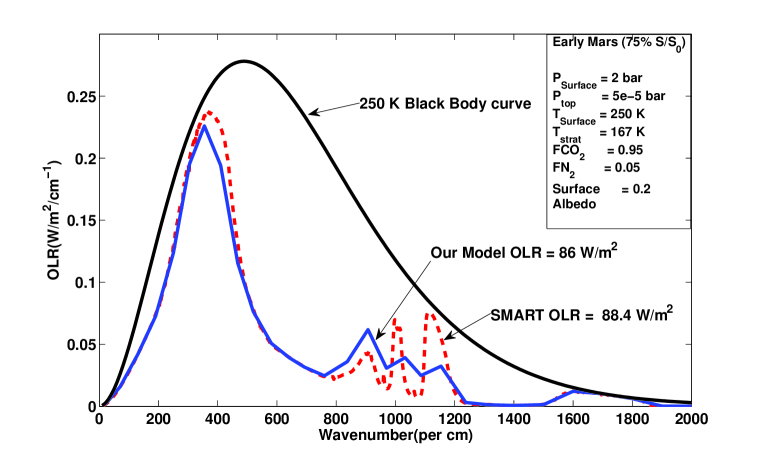
Figure 1: Plot of outgoing long-wave radiation vs. wavenumber for the $0-2000$cm^-1 region comparing our OLR (blue solid curve) to that from SMART (red dashed curve). This calculation is for early Mars conditions, 2 bar $\rm{CO_{2}}$, and constant stratospheric and surface temperatures of 167 and 250 K, respectively. The corresponding 250 K black body curve is shown in black. The integrated flux over all bands at the top of the atmosphere is $86$ Wm^-2 for our model and $88.4$ Wm^-2 for SMART.

2.2.2 Dense $\rm{H_{2}O}$ atmosphere

The inner edge of the HZ in our model is determined by the so-called “moist greenhouse effect”, in which the stratosphere becomes water-dominated, leading to rapid escape of hydrogen to space. Fig. 2 shows the net outgoing IR as a function of wavenumber for a dense $\rm{H_{2}O}$ atmosphere. Here, we assumed an Earth-mass planet with a surface temperature of $400$ K and a surface albedo of $0.3$. The stratospheric temperature is assumed to be constant at $200$ K. The stratosphere becomes tenuous at these high surface temperatures and has little effect on the outgoing IR flux. The background gas is $4$ bar of N₂ and the total surface pressure is $6.5$ bar (These conditions were assumed for specific intercomparison with SMART for this test case). The flux incident at the top of the atmosphere is assumed to be the current solar flux at Earth’s distance from the Sun.

As with the dense $\rm{CO_{2}}$ case, in Fig. 2 we compare our model (solid blue curve) with SMART (dashed red curve) for the dense $\rm{H_{2}O}$ atmosphere. Although both model spectra appear to be in good agreement, the integrated flux over all bands at the top of the atmosphere from our model is $285$ Wm^-2 compared to $297$ Wm^-2 from SMART. The differences arise in the window region of the water vapor ($800-1200$ cm^-1) and also in between $300-600$ cm^-1, where our model absorbs more than SMART. A possible reason is that we are using the BPS continuum, as opposed to the ’CKD’ continuum (Clough et al., 1989) used by SMART. The BPS formalism is based on empirical measurements which take into account the contribution of dimers, resulting in more absorption of outgoing IR radiation (see Paynter & Ramaswamy (2011) Table 3; Shine et al. (2012)).

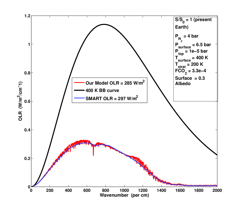
Figure 2: Plot of outgoing long-wave radiation vs. wavenumber for the $0-2000$ cm^-1 region comparing our OLR (blue solid curve) to that from SMART (red dashed curve). This calculation is for a dense $\rm{H_{2}O}$ atmosphere with stratospheric and surface temperatures of 200 K and 400 K, respectively. The corresponding 400 K blackbody curve is shown in black. Both the models appear to be in good agreement. The integrated flux over all bands at the top of the atmosphere is $285$ Wm^-2 for our model and $297$ Wm^-2 for SMART, with differences possibly arising from different formalisms of continuum absorption (BPS versus CKD. See text for details).

3 Results

In the subsections that follow, we estimate HZ boundaries around a star similar to our Sun. We first compare results from our model using HITRAN and HITEMP databases, estimate HZ limits for non-Earth-like planets and discuss the effect of clouds on the HZ boundaries.

3.1 Inner Edge of the HZ (IHZ)

The inner edge of the HZ is calculated by increasing the surface temperature of a fully saturated “Earth” model from $220$ K up to $2200$ K. The effective solar flux $S_{eff}$, which is the value of solar constant required to maintain a given surface temperature, is calculated from the ratio between the net outgoing IR flux $F_{IR}$ and the net incident solar flux $F_{SOL}$, both evaluated at the top of the atmosphere. The total flux incident at the top of the atmosphere is taken to be the present solar constant at Earth’s orbit $1360$ Wm^-2. The planetary albedo is calculated as the ratio between the upward and downward solar fluxes.

The calculated radiative fluxes, planetary albedo and water vapor profile for various surface temperatures are shown in Fig. 3. Absorption coefficients derived from the HITEMP 2010 database, overlaid by BPS formalism (Paynter & Ramaswamy, 2011), were used in generating these results. Fig. 3 shows that $F_{IR}$ increases with surface temperature and then levels out at 291 Wm^-2, as the atmosphere becomes opaque to infrared radiation at all wavelengths. Beyond 2000 K, $F_{IR}$ increases again as the lower atmosphere and surface begin to radiate in the visible and near-IR, where the water vapor opacity is low. $F_{SOL}$ initially increases as a consequence of absorption of near-IR solar radiation by $\rm{H_{2}O}$. It then decreases to a constant value ($264$ Wm^-2) at higher temperatures as Rayleigh scattering becomes important. Planetary albedo (Fig. 3) provides an alternative way of understanding this behavior. It goes through a minimum at a surface temperature of  400 K, corresponding to the maximum in $F_{SOL}$, and then flattens out at a value of 0.193.

The inner edge of the HZ for our Sun can be calculated from Fig. 3. The behavior of $F_{IR}$ and $F_{SOL}$ causes $S_{eff}$ to increase initially and then remain constant at higher temperatures. Two limits for the IHZ boundary can be calculated. The first one is the “moist greenhouse” (or water-loss) limit which is encountered at a surface temperature of $340$ K when $S_{eff}=1.015$. At this limit, the water vapor content in the stratosphere increases dramatically, by more than an order of magnitude, as shown in Fig. 3. This is the relevant IHZ boundary for habitability considerations, although it should be remembered that the actual inner edge may be closer to the Sun if cloud feedback tends to cool the planet’s surface, as expected. The orbital distance corresponding to the cloud-free water loss limit is $d=1/S_{eff}^{0.5}=0.99$ AU for an Earth-like planet orbiting the Sun.

The second IHZ limit is the runaway greenhouse at which the oceans evaporate entirely. The limiting $S_{eff}$ from Fig. 3 is 1.06 which corresponds to a distance of 0.97 AU. Both calculated IHZ limits are significantly farther from the Sun than the values found by Kasting et al. (1993) ($0.95$ AU for the water-loss limit and $0.84$ AU for the runaway greenhouse). The difference is caused by increased atmospheric absorption of incoming solar radiation by $\rm{H_{2}O}$ in the new model. As pointed out by Kasting et al. (1993), a third estimate for the IHZ boundary can be obtained from radar observations of Venus by Magellan spacecraft, which suggest that liquid water has been absent from the surface of Venus for at least 1 Gyr (Solomon & Head, 1991). The Sun at that time was $\sim 92\%$ of the present day luminosity, according to standard stellar evolutionary models (Baraffe et al., 1998; Bahcall et al., 2001, See Table 2). The current solar flux at Venus distance is $1.92$ times that of Earth. Therefore, the solar flux received by Venus at that time was $0.92\times 1.92=1.76$ times that of Earth. This empirical estimate of the IHZ edge corresponds to an orbital distance of $d=(1/1.76)^{0.5}=0.75$ AU for the present day. Note that this distance is greater than Venus’ orbital distance of 0.72 AU because the constraint of surface water was imposed at an earlier time in the planet’s history.

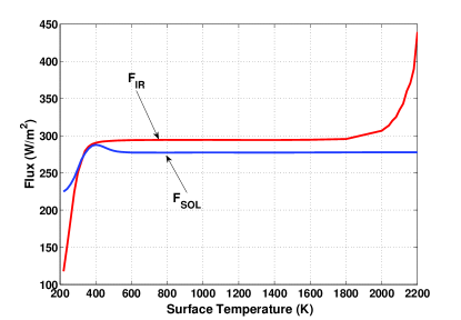
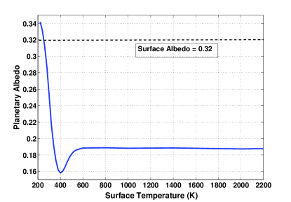
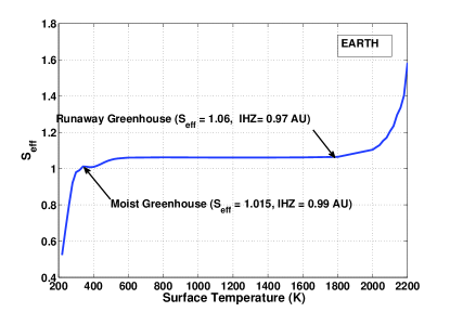
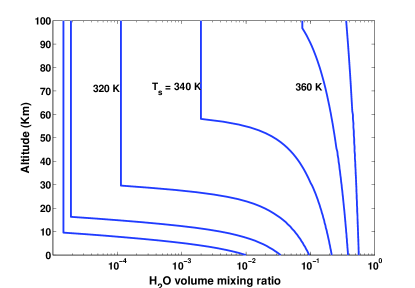
Figure 3: Inner edge of the habitable zone calculations from our updated climate model. Various parameters are shown as a function of surface temperature: (a) Net outgoing IR flux and net incident solar flux (b) planetary albedo (c) Effective solar flux, $S_{eff}=F_{IR}/F_{SOL}$, and (d) water vapor profile. These calculations were performed with the HITEMP 2010 database. The water-loss (moist greenhouse) limit, which is most relevant to habitability, is at 0.99 AU and runaway greenhouse is at 0.97 AU. The corresponding estimates from Kasting et al. (1993) climate model are 0.95 AU for the moist greenhouse and 0.84 AU for the runaway greenhouse.

3.2 Comparison of inner edge results using the HITEMP and HITRAN databases

In Fig. 4 we show $F_{IR}$ as a function of surface temperature (similar to Fig. 3). We wish to compare the outgoing IR calculated from HITRAN & HITEMP databases with and without overlaying the continuum absorption. Fig. 4 shows two significant differences:

1. The limiting value of $F_{IR}$ which leads to a runaway greenhouse happens at a much higher value (440 Wm^-2, black & green curves) when the BPS $\rm{H_{2}O}$ continuum formalism is not implemented, and at a lower $F_{IR}$ (291 Wm^-2, red & blue curves) when the BPS continuum is included in our model. The continuum is based on measurements of absorption in the water vapor window regions (i.e $800-1200$ cm^-1 and $2000-3000$ cm^-1). At high temperatures, the contribution of the continuum absorption in these window regions becomes significant, and this, in turn, decreases the outgoing IR flux.

2. The moist-greenhouse (water loss) limit moves much closer to the Sun (to 0.87 AU) when continuum absorption is not included, as compared to 0.99 AU when it is included in our model. This is a direct consequence of the differences in $F_{IR}$ described above: When $F_{IR}$ increases with the continuum turned off, $S_{eff}$ (ratio of $F_{IR}$ to $F_{SOL}$) increases and the IHZ distance $d=1/S_{eff}^{0.5}$ decreases. The result can be understood physically by noting that in the model where the continuum is absent, the planet needs more effective solar flux to maintain a given surface temperature because more thermal-IR radiation leaks away into space; hence, the IHZ boundary must move inward.

   A similar change can be seen in the runaway greenhouse limit: the ‘No BPS’ model transitions to runaway at a higher $S_{eff}$ than does the ‘with BPS’ model. The corresponding runaway greenhouse limit changes from 0.97 AU (with continuum absorption) to 0.76 AU (without continuum absorption). Fig. 4 also shows that the upturn in $F_{IR}$ beyond 800 K happens at lower surface temperatures when continuum absorption is not included. It should be remembered that this upturn in $F_{IR}$ happens because, as the surface warms, the region in the troposphere over which the temperature profile follows a dry adiabat expands upward, while the moist convective layer in the upper troposphere becomes thinner. Eventually, when the moist convective region (the cloud layer) begins thin enough, radiation emitted from the dry adiabatic portion of the atmosphere begins to escape to space. The dry adiabatic lapse rate is steeper than the moist adiabatic lapse rate by about a factor of 9 ($\sim 10$ K/km vs. 1.1 K/km); hence, the emitted radiation flux is much higher. This can be understood from the integrated form of Schwarzchild’s equation, which shows that the emitted flux is proportional to the temperature gradient. (See, e.g., eq. A4 in Kasting et al. (1984)) Unlike Kasting (1988), we find that the emitted flux increases at all thermal-IR wavelengths shorter than 4 $\mu$m. The amount of visible radiation emitted remains negligible for surface temperatures of 2200 K or below. Without the continuum there are fewer lines to cause absorption in these thermal-IR bands and hence a lower temperature would suffice to cause the upturn. Fig. 4 also shows that the model that includes both HITEMP & continuum (red curve) is the one that absorbs the most outgoing IR radiation (which is the one that was used to derive inner HZ limits in §3.1).

3.3 Outer Edge of the HZ (OHZ)

In determining the outer edge of the HZ, the surface temperature of an Earth-like planet with 1-bar N₂ atmosphere was fixed at 273 K and the atmospheric $\rm{CO_{2}}$ partial pressure, $p\rm{CO_{2}}$, was varied from 1 to 35 bars (the saturation vapor pressure for $\rm{CO_{2}}$ at that temperature). The stratospheric temperature was chosen as follows: The model atmosphere (Mars-like planet) in which the onset of $\rm{CO_{2}}$ condensation occurs has a cold-trap temperature of 154 K at an altitude where the ratio of the saturation vapor pressure to the ambient pressure is unity. We replace the temperature profile above this altitude with a constant temperature of 154 K. This allows us to calculate the solar flux ($S_{eff}$) required to maintain a global mean surface temperature of 273 K as explained in §3.1. Our working hypothesis is that atmospheric $\rm{CO_{2}}$ would accumulate as these planets cooled because of the negative feedback provided by the carbonate-silicate cycle. Results from our model calculations are shown in Fig. 5.

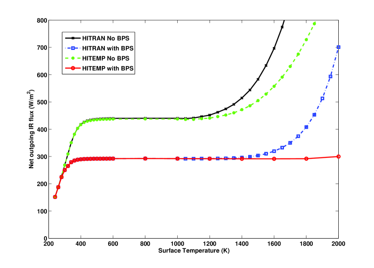
Figure 4: Comparison of outgoing IR radiation ($F_{IR}$) from HITEMP and HITRAN databases, with (blue & red curves) and without (black & green curves) continuum absorption. $F_{IR}$ is lower in the ’with BPS’ case for both the databases because the continuum absorption becomes significant in the water vapor window regions.

The incident solar ($F_{SOL}$) and outgoing IR ($F_{IR}$) fluxes are shown in Fig. 5. $F_{IR}$ decreases initially as $\rm{CO_{2}}$ partial pressure is increased; this is an indication of greenhouse effect of $\rm{CO_{2}}$. At $\sim 10$ bars, $F_{IR}$ asymptotically approaches a constant value as the atmosphere becomes optically thick at all infrared wavelengths. $F_{SOL}$ decreases monotonically with increases in $\rm{CO_{2}}$ partial pressure as a result of increased Rayleigh scattering. Correspondingly, the planetary albedo increases to high values at large $\rm{CO_{2}}$ partial pressures, as shown in Fig. 5. The solar and IR fluxes, acting in opposite directions, create a minimum of $S_{eff}=0.325$ at a $\rm{CO_{2}}$ partial pressure of $\sim 8$ bar (Fig. 5), corresponding to a distance $d=1.70$ AU. This defines the maximum greenhouse limit on the outer edge of the HZ. By comparison, Kasting et al. (1993) model predicted $d=1.67$ AU for the maximum greenhouse limit. As emphasized earlier, radiative warming by $\rm{CO_{2}}$ clouds is neglected here, even though they should be present in this calculation. Therefore, our OHZ limit should be considered as a conservative estimate, that is, the real outer edge is probably farther out.

As with the inner edge model, a more optimistic empirical limit on the OHZ can be estimated based on the observation that early Mars was warm enough for liquid water to flow on its surface (Pollack et al., 1987; Bibring et al., 2006). Assuming the dried up riverbeds and valley networks on martian surface are 3.8 Gyr old, the solar luminosity at that time would have been $\sim 75\%$ of the present value (See Eq.(1) in Gough (1981) and Table 2 in Bahcall et al. (2001)). The present-day solar flux at Mars distance is $0.43$ times that of Earth. Therefore, the solar flux received by Mars at 3.8 Gyr was $0.75\times 0.43=0.32$ times that of Earth. The corresponding OHZ limit today, then, would be $d=(1/0.32)^{0.5}\approx 1.77$ AU.

Note that this distance exceeds the maximum greenhouse limit of 1.70 AU estimated above indicating that to keep early Mars wet, additional greenhouse gases other $\rm{CO_{2}}$ and $\rm{H_{2}O}$ may be required. In fact, Ramirez et al. (2012a) show that a 3-bar atmosphere containing 90 percent $\rm{CO_{2}}$ and 10 percent H₂ could have raised the mean surface temperature of early Mars above the freezing point of water. The warming is caused by the collision-induced absorption due to foreign-broadening by molecular hydrogen. It should be acknowledged that some authors (e.g., Segura et al. (2002, 2008)) do not agree that early Mars must have been warm; however, in our view, these cold early Mars models do not produce enough rainfall to explain valley formation (Ramirez et al., 2012a).

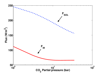
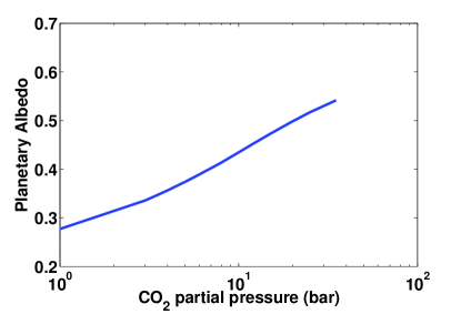
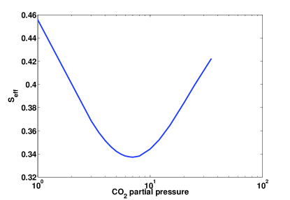
Figure 5: Outer edge of the habitable zone calculations from our climate model, shown as a function of $\rm{CO_{2}}$ partial pressure $p\rm{CO_{2}}$: (a) Net outgoing IR flux and net incident solar flux (b) planetary albedo (c) Effective solar flux. The maximum greenhouse limit, where the atmosphere becomes opaque to outgoing IR radiation, is at 1.70 AU ($S_{eff}=0.343$). The previous estimate from Kasting et al. (1993) climate model was 1.67 AU.

3.4 Effect of clouds on the HZ boundaries

We summarize various cloud-free HZ boundary estimates for Earth in Table 1. Although we updated our radiative transfer model to incorporate new absorption coefficients, this by itself may not yield a significantly better estimate for the width of the habitable zone. The reason is that it is widely acknowledged that the HZ boundaries will be strongly influenced by the presence of clouds. $\rm{H_{2}O}$ clouds should move the inner edge inwards (Kasting, 1988; Selsis et al., 2007b) because their contribution to a planet’s albedo is expected to outweigh their contribution to the greenhouse effect. (A dense $\rm{H_{2}O}$ atmosphere is already optically thick throughout most of the thermal-IR, so adding clouds has only a small effect on the outgoing IR radiation.) Conversely, $\rm{CO_{2}}$ ice clouds are expected to cause warming in a dense CO2 atmosphere because they backscatter outgoing thermal-IR radiation more efficiently than they backscatter incoming visible/near-IR radiation (Forget & Pierrehumbert, 1997). One can demonstrate the nature of these cloud influences using 1-D models, as was done in Selsis et al. (2007b). Making quantitative statements is difficult, however, because the warming or cooling effect of clouds depends on a host of parameters, including their heights, optical depths, particle sizes, and most importantly, fractional cloud coverage. Forget & Pierrehumbert (1997) obtained as much as 70 degrees of warming out of an optical depth 10 $\rm{CO_{2}}$ cloud with $100\%$ cloud cover, but that warming dropped by 30 degrees if fractional cloud cover was reduced to $75\%$. Realistic fractional cloud cover for condensation clouds is closer to $50\%$, because such clouds tend to form on updrafts, and approximately half the air in the troposphere is rising at any one time while the other half is descending.

The best way to incorporate cloud effects in a climate calculation is to use a 3-D general circulation model (GCM). Attempts were made to explain warm early mars using such 3-D models (Forget et al., 2012) but none have yet succeeded. One can, however, do significantly better than in our 1-D model, and so further research in this area is warranted (Abe et al., 2011; Wordsworth et al., 2011).

Table 1: Habitable Zone distances around our Sun from our updated 1-D climate model. For comparison, estimates from Kasting et al. (1993) are also shown.

Inner Habitable Zone                       Outer Habitable Zone
Model	Moist	Runaway	Recent Venus	Maximum	Early Mars
	greenhouse	greenhouse		greenhouse
This paper	0.99 AU	0.97 AU	0.75 AU	1.70 AU	1.77 AU
Kasting et al. (1993)	0.95 AU	0.84 AU	0.75 AU	1.67 AU	1.77 AU

3.5 Habitable Zone Limits for Non-Earth-like planets

In Table 3.5, we show the effect of surface gravities on the HZs of two planets. These planetary gravities were selected to encompass the mass range from Mars (gravity of 3.73 ms^-2) to a roughly 10 M_⊕ super-Earth (gravity of 25 ms^-2). Both planets were assumed to have a 1 bar background N₂ atmosphere. This may be unrealistic because proportionately more nitrogen is put on the smaller planet than the larger one; however, this allows direct comparison with Kasting et al. (1993). Table 3.5 shows that the habitability limits move slightly outward for a Mars-sized planet and inward for a super-Earth. This is because the column depth is larger for a Mars-sized planet, which increases the greenhouse effect (at the inner edge) and albedo (at the outer edge). Since the inner edge moves closer to the star for the super-Earth planet, while the outer edge changed little, we can conclude that, for a given surface pressure, larger planets have somewhat wider habitable zones than do small ones.

[h!] Habitable Zones around our Sun for different planetary parameters.                           Inner Habitable Zone             Outer Habitable Zone Model Moist Runaway Maximum greenhouse greenhouse greenhouse Mars-sized planet^∗ 1.035 AU 1.033 AU 1.72 AU Earth 0.99 AU 0.97 AU 1.70 AU Super-Earth^∗∗ 0.94 AU 0.92 AU 1.67 AU $p\rm{CO_{2}}=5.2\times 10^{-3}$ bar^† 1.00 AU 0.97 AU – $p\rm{CO_{2}}=5.2\times 10^{-2}$ bar 1.02 AU 0.97 AU – $p\rm{CO_{2}}=5.2\times 10^{-1}$ bar 1.02 AU 0.97 AU – $p\rm{CO_{2}}=5.2$ bar 0.99 AU 0.97 AU –

• ^∗ Surface gravity = 3.73 m.s^-2

• ^∗∗ Surface gravity = 25 m.s^-2

• ^† $p\rm{CO_{2}}=5.2\times 10^{-4}$ bar for our standard Earth model. Note that these $\rm{CO_{2}}$ pressures are not actual partial pressures; rather, they represent the surface pressure that would be produced if this amount of $\rm{CO_{2}}$ were placed in the atmosphere by itself. The 330 ppmv of $\rm{CO_{2}}$ in our standard 1-bar atmosphere would produce a surface pressure of $5.2\times 10^{-4}$ bar if the rest of the atmosphere was not present. When lighter gases such as N₂ and O₂ are present, they increase the atmospheric scale height and cause $\rm{CO_{2}}$ to diffuse upward, thereby lowering its partial pressure at the surface.

We also performed sensitivity tests on the inner edge of the HZ by varying the amount of atmospheric $\rm{CO_{2}}$ (the outer edge calculation already factors in this change in $\rm{CO_{2}}$). It is quite possible that some terrestrial planets may have varying amount of $\rm{CO_{2}}$ because of different silicate weathering rates. As shown in Table. 3.5, changes in $p\rm{CO_{2}}$ would not change the runaway greenhouse limit, as it is reached in an $\rm{H_{2}O}$-dominated atmosphere. The moist greenhouse limit does change, as an increase in $p\rm{CO_{2}}$ increases the surface temperature, and hence facilitates water loss. The maximum destabilization occurs at a $p\rm{CO_{2}}=5.2\times 10^{-3}$ bar approximately 10 times the present terrestrial $p\rm{CO_{2}}$ level (the critical distance, shown in bold in Table 3.5, is 1.00 AU).

This suggests that a 10-fold increase in $\rm{CO_{2}}$ concentration relative to today could push Earth into a moist greenhouse state (assuming a fully saturated atmosphere). By contrast, the maximum destabilization occurred at $1000$ times the present $\rm{CO_{2}}$ level in Kasting et al. (1993). At larger $p\rm{CO_{2}}$ values the increase in surface pressure outstrips the increase in the saturation vapor pressure of water, so the atmosphere becomes more stable against water loss (Kasting & Ackerman, 1986). We conclude that planets with few tenths of a bar of $p\rm{CO_{2}}$ have narrower HZs than planets like Earth on which $p\rm{CO_{2}}$ is maintained at lower values by the carbonate-silicate cycle.

4 Habitable Zones around Main-Sequence Stars

The procedure described in the previous section to derive HZs around Sun can be used to estimate HZ boundaries around stars of different spectral types. A similar analysis was done by Kasting et al. (1993) for three stellar effective temperatures (7200 K, 5700 K and 3700 K), which correspond to F0, G0, and M0 spectral types. Selsis et al. (2007b) used a similar model to that of Kasting et al. (1993) and interpolated HZ distances to stars within this range of effective temperatures. Here, we compare our updated model results with these earlier studies and also extend the calculations to lower stellar effective temperatures to include M-dwarfs. Correctly calculating HZs of M-dwarfs is becoming increasingly important, as upcoming instruments such as Penn State’s stabilized fiber-fed near-infrared (NIR) spectrograph Habitable Zone Planet Finder (HPF, Mahadevan et al. (2012)) and proposed missions such as Transiting Exoplanet Survey Satellite (TESS) will specifically search for low-mass planets around M-dwarfs. Furthermore, several rocky planets have already been found in the HZs of M-dwarfs (Bonfils et al., 2011; Vogt et al., 2012), and these objects may be good candidates for space-based characterization missions such as JWST.

4.1 Habitable Zone Boundaries Around F, G, K and M Stars

We considered stellar effective temperatures in the range $2600$ K $\leq T_{eff}\leq 7200$ K, which encompasses F, G, K and M main-sequence spectral types. As input spectra for the HZ boundary calculations we used the “BT$\_$Settl” grid of models (Allard et al., 2003, 2007). These cover the needed wavelength range for climate models (0.23-4.54 $\mu$m), as well as the range of effective temperature ($2600$ K $\leq T_{eff}\leq 70,000$ K) needed to simulate stellar spectra. Our comparison of the BT$\_$Settl models with low-resolution IRTF data, and also high-resolution CRIRES data on Barnard’s star (from the CRIRES$\_$POP library (Lebzelter et al., 2012)), show that the models are quite good in reproducing the gross spectral features and energy distributions of stars, and will provide adequate input for our HZ calculations. For each star, the total energy flux over our climate model’s spectral bands is normalized to 1360 Wm^-2 (the present solar constant for Earth) to simplify intercomparison.

In Fig. 6 we compare the results of our inner and outer edge HZ model calculations for Sun to stars of different spectral types. Unless otherwise specified, we use the HITEMP 2010 database for our inner edge calculations. The planetary albedo, shown in Fig. 6 (inner edge) and Fig. 6 (outer edge), of an Earth-like planet is higher if the host star is an F-star and lower if its primary is an M-star. The reason is that the Rayleigh scattering cross section (which is proportional to $1/\lambda^{4}$) is on average higher for a planet around an F-star, as the star’s Wien peak is bluer compared to the Sun. Second, $\rm{H_{2}O}$ and $\rm{CO_{2}}$ have stronger absorption coefficients in the near-infrared than in the visible, so the amount of starlight absorbed by the planet’s atmosphere increases as the radiation is redder (as is the case for an M-star). Both effects are more pronounced when the atmosphere is dense and full of gaseous absorbers. For a late M-star ($T_{eff}=2600$ K) most of its radiation is peaked around $1$ micron. Therefore, the minimal amount of Rayleigh scattering and the high near-IR absorption by the planet’s atmosphere combine to generate extremely low planetary albedos.

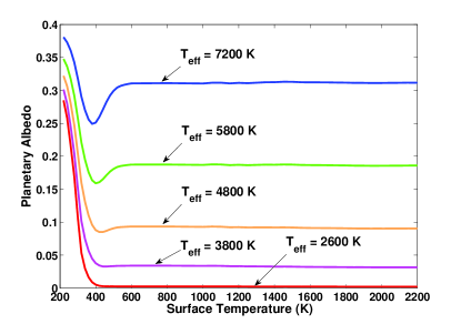
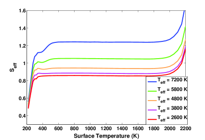
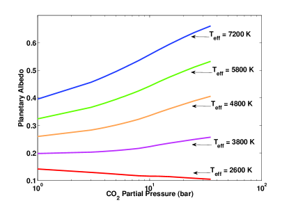
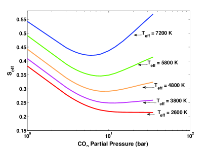
Figure 6: Habitable zone calculations from our climate model for stellar effective temperatures corresponding to F ($T_{eff}=7200$ K), G (Sun), K ($T_{eff}=4800$ K) and M ($T_{eff}=3800$ K and 2600 K) spectral types. The inner edge results are shown in the top row (Figs. 6 & 6) and the outer edge results are shown in the bottom row (Figs. 6 & 6).

The changes in predicted planetary albedo can be translated into critical solar fluxes, as shown in Figs. 6 (inner edge) and 6 (outer edge). As discussed in §3.3, $S_{eff}$ goes through a minimum near the OHZ because the atmosphere becomes optically thick at all infrared wavelengths and, at the same time, the Rayleigh scattering due to $\rm{CO_{2}}$ condensation increases planetary albedo. Note that for a late M-star ($T_{eff}=2600$ K) Rayleigh scattering never becomes an important factor, and hence $S_{eff}$ asymptotically reaches a constant value. The parameter $S_{eff}$ is directly calculated from our climate model and is dependent on the type of star considered. Therefore, we have derived relationships between HZ stellar fluxes ($S_{eff}$) reaching the top of the atmosphere of an Earth-like planet and stellar effective temperatures ($T_{eff}$) applicable in the range $2600$ K $\leq T_{eff}\leq 7200$ K.

$$S_{eff} = S_{eff\odot}+aT_{\star}+bT_{\star}^{2}+cT_{\star}^{3}+dT_{\star}^{4}$$ (2)

where $T_{\star}=T_{eff}-5780$ K and the coefficients are listed in Table 6 for various habitability limits. The corresponding habitable zone distances can be calculated using the relation:

$$d = \biggl{(}\frac{L/L_{\odot}}{S_{eff}}\biggr{)}^{0.5}\mathrm{AU}$$ (3)

where $L/L_{\odot}$ is the luminosity of the star compared to the Sun.

In Fig. 7 we compare HZ fluxes (and distances) calculated using Eqs.(2) $\&$ (3) for the moist greenhouse case, with Selsis et al. (2007b) $0\%$ cloud results for different stellar effective temperatures. As shown in Fig. 7, for low $T_{eff}$, there are large differences at the inner edge (dashed and solid red curves) between the models. This is because the spectrum of low-mass stars shifts towards the longer wavelengths, resulting in more near-IR flux compared to high-mass stars. In both the models the atmosphere of a planet in the inner HZ is $\rm{H_{2}O}$-dominated, and so there is strong absorption in the near-IR. Since our model uses the most recent HITEMP database which has more $\rm{H_{2}O}$ lines in the near-IR, the moist greenhouse limit occurs at a lower flux (farther from the star). Also, Selsis et al. (2007b) assumed $T_{eff}=3700$ K for stars with temperatures below this value. This amplifies the differences, as these low mass stars have their peak fluxes in near-IR. These differences in inner habitable zone boundaries may become important for present and upcoming planet finding surveys around M-dwarfs such as MEARTH (Nutzman & Charbonneau, 2008) and Penn State’s HPF (Mahadevan et al., 2012), whose goal is to discover potentially habitable planets around M-dwarfs.

The luminosity of a main sequence star evolves over time, and consequently the HZ distances (Eq.(3)) also change with time. One can calculate “continuous” HZ (CHZ) boundaries within which a planet remains habitable for a specified length of time (we chose 5 Gyr). In Fig. 7, we show CHZ boundaries as a function of stellar mass for both our model and Selsis et al. (2007b) model, taking into account the stellar evolutionary models of Baraffe et al. (1998) for solar metallicity stars. Noticeable differences between the two models are seen for low mass stars near the inner edge (as also seen in Fig. 7. The large differences in $S_{eff}$ from Fig. 7 do not appear as pronounced in Fig. 7 because it is a log scale and also because the CHZ distance is inversely proportional to the square root of $S_{eff}$ (Eq.(3)).

In order to assess the potential habitability of recently discovered exoplanets, equilibrium temperature ($T_{eq}$) has been used as a metric (Borucki et al., 2011; Batalha et al., 2012). Assuming an emissivity of $0.9$, the ranges of HZ boundaries are taken to be $185$ K $\leq T_{eq}\leq 303$ K (Kasting, 2011b). We would like to stress that the stellar fluxes ($S_{eff}$) provide a better metric for habitability than does $T_{eq}$. This is because $T_{eq}$ involves an assumption about $A_{B}$ ($0.3$, usually) that is generally not valid. This value of $A_{B}$ is good for present Earth around our Sun. For a planet around a late M-star, $A_{B}$ can vary from 0.01 near the inner edge to 0.1 at the outer edge (see Fig. 6), depending on its location. Similarly, $A_{B}$ for an F-star can range in between $0.38-0.51$ for the inner and outer edge, respectively. This changes the corresponding $T_{eq}$, and so a uniform criterion for HZ boundaries based on $T_{eq}$ cannot be determined.

[h!] Coefficients to be used in Eq.(2) to calculate habitable stellar fluxes, and corresponding habitable zones (Eq.(3)), for stars with $2600\leq T_{eff}\leq 7200$ K. An ASCII file containing these coefficients can be downloaded in the electronic version of the paper. Constant Recent Runaway Moist Maximum Early Venus Greenhouse Greenhouse Greenhouse Mars $S_{eff\odot}$ 1.7753 1.0512 1.0140 0.3438 0.3179 $a$ $1.4316\times 10^{-4}$ $1.3242\times 10^{-4}$ $8.1774\times 10^{-5}$ $5.8942\times 10^{-5}$ $5.4513\times 10^{-5}$ $b$ $2.9875\times 10^{-9}$ $1.5418\times 10^{-8}$ $1.7063\times 10^{-9}$ $1.6558\times 10^{-9}$ $1.5313\times 10^{-9}$ $c$ $-7.5702\times 10^{-12}$ $-7.9895\times 10^{-12}$ $-4.3241\times 10^{-12}$ $-3.0045\times 10^{-12}$ $-2.7786\times 10^{-12}$ $d$ $-1.1635\times 10^{-15}$ $-1.8328\times 10^{-15}$ $-6.6462\times 10^{-16}$ $-5.2983\times 10^{-16}$ $-4.8997\times 10^{-16}$

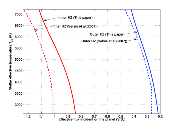
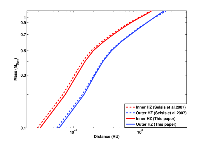
Figure 7: Habitable zone fluxes (panel 7) and corresponding distances (panel 7) from our model (solid lines) compared to Selsis et al. (2007b) results (dashed lines) for different stellar effective temperatures. The inner HZ fluxes from our model (red solid lines) are for the moist greenhouse case and outer edge fluxes (blue solid lines) are for the maximum greenhouse limit, which are compared with $0\%$ cloud cover limit from Table 2 of Selsis et al. (2007b). The corresponding continuous HZ distances for 5 Gyr are shown in panel 7.

5 Discussion

A straightforward application of the calculations presented in the previous sections is to apply them to currently known exoplanetary systems. Fig. 8 shows various habitable zone boundaries (expressed in terms of effective stellar flux) as a function of stellar $T_{eff}$. The orbital parameters of the planets and stellar characteristics were obtained from exoplanets.org (Wright et al., 2011). The green-shaded habitable region is bounded by the moist greenhouse limit (inner edge) and the maximum greenhouse limit (outer edge). Several currently known terrestrial mass exoplanets that have been proposed to be in the HZ by various studies are also shown. An important insight that can be obtained from this figure (and one that cannot be seen in the HZ distance plot, Fig. 7) is that a terrestrial mass planet that lies within the two vertical dashed-lines in the green shaded region is in the HZ irrespective of the type of star it is orbiting. The corresponding flux boundaries for which a rocky planet is ‘definitely’ in the HZ are $0.842$ and $0.42$. Currently, two exoplanets fall within this region, HD 40307g (Tuomi et al., 2012a) and Gl 581g (Vogt et al., 2010, 2012). The detection of planets and orbital parameters for Gl581 is complicated by the low amplitudes of the signal, stellar activity, and possible red noise. We have included a ‘?’ for Gl 581 system of planets in the plot, indicating that there is an active ongoing discussion in the literature about the number of planets in this system and their exact orbital parameters (Vogt et al., 2010; Pepe et al., 2011b; Vogt et al., 2012; Baluev, 2012). Furthermore, for stars with T${}_{eff}\lesssim 5000$ K, there is no clear distinction between runaway greenhouse and the moist-greenhouse limits. The reason is that for these stars, there are more photons available in the IR part of the spectrum, where $\rm{H_{2}O}$ is a good absorber. Therefore a planet with $\rm{H_{2}O}$ dominated atmosphere quickly goes into runaway once it reaches the moist-greenhouse limit. Note that another suggested HZ candidate planet, HD 85512b (Pepe et al., 2011a), receives more than 5 times the stellar flux received by our Earth, placing it even beyond the most liberal (‘recent Venus’) estimate of the inner edge. Hence, it is very likely that this planet is not in the HZ of its star.

A question of importance to the exoplanet community is which HZ limits to choose when identifying potentially habitable planets. For current RV surveys and Kepler mission one should use the most conservative limits (moist greenhouse and maximum greenhouse), because this will give a lower limit on $\eta_{\oplus}$, the fraction of sun-like stars that have at least one planet in the habitable zone (Luinine et al., 2008). If one is interested in designing a future flagship mission, such as Terrestrial Planet Finder (TPF) or Darwin, then using these conservative limits (which results in a lower limit on $\eta_{\oplus}$) ensures that the telescope is not undersized. If, however, one was analyzing data obtained from such a telescope, the most optimistic limits (recent Venus and early Mars) should be used because one would not want to miss out on any potentially habitable planets.

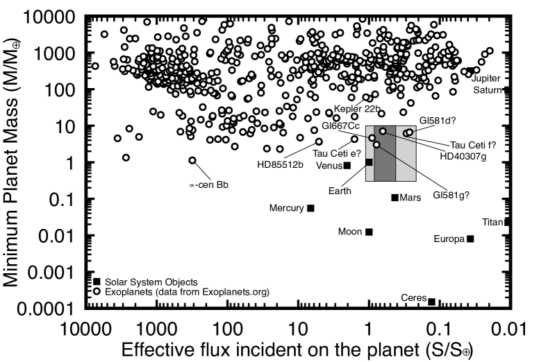
Figure 9: HZ boundaries combining observable stellar and planetary parameters. Terrestrial planets ($0.3$M_⊕ - $10$M_⊕, y-axis limits) within the dark shaded region are in the HZ irrespective of the stellar type. For those planets in the light grey region, one needs to know the stellar type to determine if they are in the HZ. For example, the Earth would not be habitable if it received its current incoming amount of energy from a cooler-type star, but it is (obviously) habitable in its current orbit around a G-type star. For planets such as this, the star’s energy distribution matters when considering habitability.

In Fig. 9, we show the incident stellar flux as a function of planetary mass for the currently known exoplanets. The masses are obtained from exoplanets.org when available. Also shown are habitable zone flux boundaries calculated from Eq.(2) for terrestrial mass planets ($1$M_⊕ - $10$M_⊕). For the outer box (light grey), the upper bound on the flux is taken to be the moist greenhouse limit for a star with $T_{eff}=7200$ K and the lower bound is the maximum greenhouse limit for a star with $T_{eff}=2600$ K. These are indicated by the diagonally opposite points on the green shaded region in Fig. 8. For the inner box (dark grey), the flux limits are the dashed lines in the green shaded region of Fig. 8. The significance of this plot is that terrestrial planets in the inner box must be in the HZ, irrespective of the stellar spectral type. Mars, if it were more massive, would be in the HZ around any main sequence star with $2600\leq T_{eff}\leq 7200$ K. For planets that are outside the dark grey region, but inside the light grey (for example, Earth) one needs to know the host star’s spectral type (or $T_{eff}$) to determine if that planet is in the HZ. Fig. 9 combines observable stellar and planetary parameters to further constrain HZ boundaries for extrasolar planets.

Many of the currently known exoplanets have non-zero eccentricities, which can carry some of them (and their possible moons) in and out of the HZ. The incident stellar flux on these eccentric planets has extreme variations between periastron and apoastron ($[(1+e)/(1-e)]^{2}$). Williams & Pollard (2002) show that, provided that an ocean is present to act as a heat capacitor, it is primarily the time-averaged flux $<S_{eff}^{~{}\prime}>$ that affects the habitability over an eccentric orbit (Kopparapu et al., 2009; Kopparapu & Barnes, 2010). Mathematically:

$$<S_{eff}^{~{}\prime}> = \frac{S_{eff}}{(1-e^{2})^{1/2}}$$ (4)

Here, $S_{eff}$ is the effective flux from circular orbit (Eq.(2)). Planets with high orbital eccentricities ($e\sim\geq 0.1$) have higher average orbital flux. This may help eccentric planets near the outer edge of the HZ maintain habitable conditions. However, obliquity variations can influence the geographical distribution of irradiation (Spiegel et al., 2008, 2009; Dressing et al., 2010) and may change habitable conditions.

Earth itself appears to be perilously close to the moist greenhouse limit ($S_{eff}=1.015$, blue filled circle in Fig. 8). However, this apparent instability is deceptive, because the calculations do not take into account the likely increase in Earth’s albedo that would be caused by water clouds on a warmer Earth. Furthermore, these calculations assume a fully saturated troposphere that maximizes the greenhouse effect. For both reasons, it is likely that the actual HZ inner edge is closer to the Sun than our moist greenhouse limit indicates. Note that the moist greenhouse in our model occurs at a surface temperature of 340 K. The current average surface temperature of the Earth is only 288 K. Even a modest (5-10 degree) increase in the current surface temperature could have devastating affects on the habitability of Earth from a human standpoint. Consequently, though we identify the moist greenhouse limit as the inner edge of the habitable zone, habitable conditions for humans could disappear well before Earth reaches this limit.

Additional uncertainty about habitability of planets around late-K and M stars. ($T_{eff}<=4000$ K) comes from the fact that planets within the HZs of these stars are expected to be tidally locked (Dole, 1964; Peale, 1977; Kasting et al., 1993; Dobrovolskis, 2009). If the planet’s orbital eccentricity is small, this can result in synchronous rotation, in which one side of a planet always faces the star (as the Moon does to the Earth). Climates of synchronously rotating planets are not well approximated by 1-D, globally averaged models. Previous work has shown that such planets may indeed be habitable (Joshi et al., 1997; Joshi, 2003; Edson et al., 2003); however, systematic exploration of synchronously rotating planets in different parts of the HZ has not been attempted. Even before doing these calculations, we can predict that planets near the outer edge of the HZ, with their expected dense $\rm{CO_{2}}$ atmospheres, should be more effective at transporting heat around to their night sides, and hence should have a better chance of being habitable.

Given that survey like HPF and CARMENES will specifically target mid-late M dwarfs, our future work will include estimating the HZ boundaries of individual targets in detail. Ongoing work by our team (Terrien et al., 2012) is yielding low resolution NIR spectra from the infrared Telelescope Facility (IRTF) to be used to derive stellar metallicities as well as yielding more realistic flux distributions and temperatures for use in the modeling. We anticipate having this information for $\sim$ 650 M dwarfs drawn from the J$<10$ Lepine & Gaidos (2011)catalog, and have applied for time to observe $\sim$ 300 more. Estimates of luminosities will be derived using photometric and spectroscopic distances for now (in cases where parallax measurements are absent), but eventually GAIA (Perryman et al., 2001) will yield very precise parallaxes (and by extension precise luminosities) for all these target stars.

Recent discoveries by both the Kepler mission and RV surveys have shown that planets can exist in stable orbits around multiple star systems (Doyle et al., 2011; Welsh et al., 2012; Orosz et al., 2012; Dumusque et al., 2012). The HZs of these stars could potentially host terrestrial planets, which are at the threshold of current detection techniques. Indeed, the discovery of Kepler 47c (Orosz et al., 2012) which is 4.6 times the size of the Earth’s radii in the HZ is a step closer to discovering rocky planets in the HZ of multiple star systems. Dumusque et al. (2012) have recently published a possible detection of a 1.1 Earth mass (minimum) planet in a 3.236 day orbit around $\alpha$ Centauri system. So, this system should now be a prime target for further observations to discover habitable planets. Formation of dynamically stable terrestrial planets in the HZs of multiple star systems has been studied before (Whitmire et al., 1998; Holman & Wiegert, 1999; Haghighipour & Raymond, 2007) and several studies estimated HZ boundaries around these types of systems (Eggl et al., 2012a, b; Kane & Hinkel, 2012) using Kasting et al. (1993) model. Our updated model results from Fig. 8 or Eqs.(2) and (3) could change these estimates significantly.

Our new model results could also directly affect estimates of $\eta_{\earth}$. Recent analysis of Kepler data (Traub, 2012) and RV surveys (Bonfils et al., 2011) concluded that $\eta_{\earth}\sim 0.34-0.4$. These values were based either on the Kasting et al. (1993) model (Traub, 2012) or the Selsis et al. (2007b) results (Bonfils et al., 2011). Our new HZ limits could impact these estimates significantly. In particular, there are large differences between Selsis et al. (2007b) calculations and our model results for low mass stars. The estimate of $\eta_{\earth}$ by Bonfils et al. (2011) is obtained by using Selsis et al. (2007b) relationships for planets orbiting M-stars. Thus, this value may need to be re-evaluated.

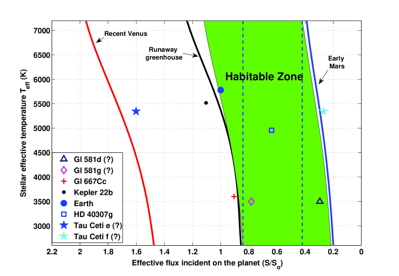
Figure 8: Various cloud-free habitable zone (flux) boundaries for stars with different $T_{eff}$. The boundaries of the green-shaded region are determined by the moist-greenhouse (inner edge, higher flux values) & maximum greenhouse (outer edge, lower flux values). A planet that receives stellar flux bounded by the two dashed vertical lines is in the HZ irrespective of the stellar type. Some of the currently known exoplanets that are thought to be in the HZ by previous studies are also shown. The ‘?’ for Gl 581 and Tau Ceti system of planets imply that there is an ongoing discussion about their existence. For stars with T${}_{eff}\lesssim 5000$ K, there is no clear distinction between runaway and moist-greenhouse limit.

6 Conclusions

We have obtained new estimates for HZs around F, G, K and M main-sequence stars by (1) updating $\rm{H_{2}O}$ and $\rm{CO_{2}}$ absorption coefficients in the Kasting et al. (1993) 1-D radiative-convective cloud-free climate model with the most recent LBL databases: HITRAN 2008 and HITEMP 2010, (2) correcting the $\rm{H_{2}O}$ Rayleigh scattering coefficient, and (3) updating $\rm{CO_{2}}$ collision-induced absorption coefficients. These changes affect the inner and outer edges of the HZ, respectively.

Our revised model predicts that the moist greenhouse limit for our Sun, which defines the inner edge of the HZ, is at 0.99 AU. The outer edge of the HZ, where gaseous $\rm{CO_{2}}$ produces its maximum greenhouse effect, is at 1.70 AU. Although it appears that Earth is perilously close to the inner HZ edge, in reality, cloud feedback and low upper tropospheric relative humidity act to stabilize Earth’s climate. Theoretical studies and observational surveys that depend on these limits should use the updated values. We have also estimated HZ boundaries for M stars with $T_{eff}$ as low as $2600$ K, which are primary targets for ongoing surveys such as Habitable Zone Planet Finder and MEARTH to discover potential habitable planets.

We also showed that the effective stellar flux provides a better criterion in determining the HZ limits, than equilibrium temperature. Accordingly we have derived a generalized expression to calculate these fluxes for stars of different spectral types. Our results show that some of the extrasolar planets that were previously thought to be within the HZ may not be in that region. Thus, our HZ estimates can be used to narrow the target list for eventual characterization missions, such as JWST, to identify potential biomarkers on habitable planets.

Author Contribution: R.K & R.R contributed equally to this work. An interactive webpage to obtain HZs and a FORTRAN code is available here: http://depts.washington.edu/naivpl/content/hz-calculator. The FORTRAN code is also available in the electronic version of the paper.

References

- Abbot et al. (2012) Abbot,D. S., Cowan, N. B., & Ciesla, F. J. 2012. ApJ, 756, article id. 178
- Abe et al. (2011) Abe, Y., Abe-Ouchi, A., Sleep, N. H., & Zahnle, K. J. 2011. Astrobiology, 11, 443
- Allard et al. (2003) Allard, F., Guillot, T., & Ludwig, H. G. et al. 2003, Brown Dwarfs, Proceedings of IAU Symposium, 211, 20-24 May, 2002, University of Hawaii, Honolulu, Hawai
- Allard et al. (2007) Allard, F., Allard, N. F., & Homeier, D. et al. 2007, A&A, 474, L21
- Allen (1976) Allen, C. 1976, Astrophysical Quantities (University of London: The Athlone Press)
- Bahcall et al. (2001) Bahcall, J. N., Pinsonneault, M. H., & Basu, Sarbani. 2001. ApJ, 555, 990
- Baluev (2012) Baluev, R. V. 2012. submitted to MNRAS.
- Baranov et al. (2004) Baranov. Y. I., Lafferty, W. J., & Fraser, G. T. 2004. Journal of Molecular Spectroscopy, 228, 432
- Baraffe et al. (1998) Baraffe, I., Chabrier, G., Allard, F., & Hauschildt, P. 1998, A&A, 337, 403
- Batalha et al. (2012) Batalha, N. M., Rowe, J. F., Bryson, S. T. et al. 2012. submitted to ApJS, arXiv:1202.5852
- Bender et al. (2012) Bender, C. F., Mahadevan, S., Deshpande, R. 2012. ApJ, 751, L31
- Bezard et al. (1990) Bezard, B., Debergh, C., Crisp, D., & Maillard, J. P. 1990, Nature, 345, 508
- Bibring et al. (2006) Bibring, J.-P., Langevin, Y., Mustard, J. F., et al. 2006, Science, 312, 400
- Bonfils et al. (2011) Bonfils, X., Delfosse, X., Udry, S. et al. 2011. submitted A&A, arXiv:1111.5019
- Borucki et al. (2011) Borucki, W. J., Koch, D. G., Basri, G. et al. 2011. ApJ, 736, article id. 19
- Borucki et al. (2012) Borucki, W. J., Koch, D. G., Batalha, N. et al. 2012. ApJ, 745, article id. 120
- Bucholtz (1995) Bucholtz, A. 1995, Appl. Opt., 34, 2765
- Burch et al. (1969) Burch, D. E., Gryvnak, D. A., Patty, R. R., & Bartky, C. E. 1969. Opt. Soc. Am., 59, 267
- Clampin et al. (2007) Clampin, M., Valenti, J., Deming, D. 2007. Detection of Planetary Transits with the James Webb Space Telescope. ExoPTF whitepaper.
- Clough et al. (1989) Clough, S. A., Kneizys, F. X., and Davies, R. W. 1989. Atmospheric Research, 23, 229
- Clough & Iocono (1995) Clough, S. A., & Iacono, M. J. 1995. J. Geophys. Res, 100, 16519
- Colaprete & Toon (2003) Colaprete, A., & Toon, O. B. 2003. Journal of Geophysical Research (Planets), 108, 6-1
- Crisp (1997) Crisp, D. 1997. Geophysical Research Letters, 24, 571
- Deming et al. (2009) Deming, D., Seager, S., Winn, J. et al. 2009. PASP, 121, 952
- Dobrovolskis (2009) Dobrovolskis, A. R. 2009. Icarus, 204, 1
- Dole (1964) Dole, S. H. 1964. Habitable Planets for Man. New York: Blaisdell Publishing. 158 pp
- Doyle et al. (2011) Doyle, L. R., Carter, J. A., Fabrucky, D. C. et al. 2011. Science, 333, 1602
- Dressing et al. (2010) Dressing, C. D., Spiegel, D. S., Scharf, C. A., Menou, K., & Raymond, S. N. 2010. ApJ, 721, 1295
- Dumusque et al. (2012) Dumusque, X., Francesco, P., Christophe, L. et al. 2012. Nature, doi:10.1038/nature11572
- Edlén (1996) Edlén, B. 1966. Metrologia, 2, 71
- Edson et al. (2003) Edson, A., Lee, S., Bannon, P., Kasting, J. F., & Pollard, D. 2011. Icarus, 212, 1
- Eggl et al. (2012a) Eggl, S., Pilat-Lohinger, E., Georgakarakos, N. et al. 2012. ApJ, 752, article id. 74
- Eggl et al. (2012b) Eggl, S., Pilat-Lohinger, E., Funk, B. 2012. arXiv:1210.5411
- Forget & Pierrehumbert (1997) Forget, F., & Pierrehumbert, R.T., 1997. Science, 278, 1273
- Forget et al. (2012) Forget, F., Wordsworth, R. W., Millour, E. et al. 2012. Icarus accepted. arXiv:1210.4216
- Fukabori et al. (1986) Fukabori, M., Nakazawa, T., & Tanaka, M. 1986. JQSRT, 36, 265
- Goldblatt & Zahnle (2011) Goldblatt, C., & Zahnle, K. 2011. Nature, 474, 7349
- Gough (1981) Gough, D. O. 1981. ESA and European Physical Society, ESLAB Symposium on Physics of Solar Variations, 14th, Scheveningen, Netherlands. Solar Physics, 74, 21
- Gruszka & Borysow (1994) Gruszka, M. & Borysow, A. 1994. J. Chem. Phys, 101, 3573
- Gruszka & Borysow (1997) Gruszka, M. & Borysow, A. 1997. Icarus, 129, 172
- Haghighipour & Raymond (2007) Haghighipour, N., & Raymond, S. 2007, ApJ, 666, 436
- Halevy et al. (2009) Halevy, I., Pierrehumbert, R. T., & Schrag, D. P. 2009. Journal of Geophysical Research, 114, D18112
- Haqq-Misra et al. (2008) Haqq-Misra, J. D., Domagal-Goldman, S. D., Kasting, P. J. & Kasting, J. F. 2008. Astrobiology, 8, 1127
- Hart (1978) Hart, M. H. 1978, Icarus, 33, 23
- Holman & Wiegert (1999) Holman, M .J., & Wiegert, P. A. 1999. AJ, 117, 621
- Huang (1959) Huang, S. S. 1959, American Scientist, 47, 397
- Joshi et al. (1997) Joshi, M. M., Haberle R. M., Reynolds R. T. 1997. Icarus, 129, 450
- Joshi (2003) Joshi, M. M. 2003. Astrobiology, 3, 415
- Kaltengger & Traub (2009) Kaltenegger, L., & Traub, W. 2009. ApJ. 698, 519
- Kaltenegger et al. (2011a) Kaltenegger, L., Segura, A., & Mohanty, S. 2011a. ApJ. 733. id. 35
- Kaltenegger et al. (2011b) Kaltenegger, L., & Sasselov, D. 2011b. ApJ, 736, L25
- Kane & Hinkel (2012) Kane, S. R, & Hinkel, N. R. 2012. ApJaccepted. arXiv:1211.2812
- Kasting et al. (1984) Kasting, J. F., Pollack, J. B., Crisp, D. 1984. J. Atmos. Chem., 1, 403
- Kasting & Ackerman (1986) Kasting, J. F., & Ackerman, T. P. 1986. Science, 234, 1383
- Kasting (1988) Kasting, J., F. 1988, Icarus, 74, 472
- Kasting (1991) Kasting, J., F. 1991, Icarus, 94, 1
- Kasting et al. (1993) Kasting, J., F., Whitmire, D., P., & Reynolds. R. T. 1993, Icarus, 101, 108
- Kasting (2011b) Kasting, J. F. 2011b. Joint Meeting of the Exoplanet and Cosmic Origins Program Analysis Groups (ExoPAG and COPAG), April 26, 2011, Baltimore, MD, http://exep.jpl.nasa.gov/exopag/exopagCopagJointMeeting/
- Kato et al. (1999) Kato, S., Ackerman, T. P., Mather, J. H. et al. 1999. J. Quant. Spectrosc. Radiat. Transf., 62, 109
- Kitzmann et al. (2011a) Kitzmann, D., Patzer, A. B. C., Von Paris, P. P., Godolt, M., & Rauer, M. 2011a. A&A. 531, id.A62
- Kitzmann et al. (2011b) Kitzmann, D., Patzer, A. B. C., Von Paris, P. P., Godolt, M., & Rauer, M. 2011b. A&A. 534, id.A63
- Kopparapu et al. (2009) Kopparapu, R., Raymond, S. N., Barnes, R. 2009. ApJ, 695, L181
- Kopparapu & Barnes (2010) Kopparapu, R. & Barnes, R. 2010. ApJ, 716, 1336
- Lebzelter et al. (2012) Lebzelter, T., Seifahrt, A., Uttenthaler, S. et al. 2012. A&A, 539, 25
- Lepine & Gaidos (2011) Lepine, S., & Gaidos, E. 2011. AJ, 142, 15
- Luinine et al. (2008) Lunine, J. I., Fischer, D., Hammel, H. B. 2008. Astrobiology, 8, Issue 5
- Mahadevan et al. (2012) Mahadevan, S., Ramsey, L., Bender, C. et al. 2012.To appear in the proceedings of the SPIE2012 Astronomical Instrumentation and Telescopes conference arXiv:1209.1686
- Manabe & Wetherald (1967) Manabe, S., & Wetherald, R. T. 1967. Journal of Atmospheric Science, 24, 241
- Marshall & Smith (1990) Marshall, B. R., & Smith, R. C. 1990, Appl. Opt., 29, 71
- Meadows & Crisp (1996) Meadows, V. S., & Crisp, D. 1996. Journal of Geophysical Research, 101, 4595
- Mischna et al. (2000) Mischna, M.A., Kasting, J.F., Pavlov, A., Freedman, R., 2000. Icarus, 145, 546
- Mlawer et al. (1997) Mlawer, E. J., Taubman, S. J., Brown, P. D. et al. 1997. J. Geophys. Res., 102, 16663
- Nutzman & Charbonneau (2008) Nutzman, P., & Charbonneau, D. 2008. Publications of the Astronomical Society of the Pacific, 120, 317
- Orosz et al. (2012) Orosz, J. A., Welsh, W. F., Carter, J. A. et al. 2012. Science, 337, 1511
- Paynter & Ramaswamy (2011) Paynter, D. J. & Ramaswamy, V. 2011. Journal of Geophysical Research-Atmospheres, 116, D20302
- Peale (1977) Peale, S. J. 1977. Rotational histories of the natural satellites. In Planetary Satellites , ed. J. A. Burns. Tucson, AZ: University of Arizona Press
- Pepe et al. (2011a) Pepe, F., Lovis, C., Segransan, D. et al. 2011a. A&A, 534, A58
- Pepe et al. (2011b) Pepe, F., Mayor, M., & Lovis, C. et al. 2011b. in: A. Sozzetti, M.G. Lattanzi, A.P. Boss (eds.), The astrophysics of planetary systems: formation, structure, and dynamical evolution, IAU Symp. 276, p. 13
- Perrin & Hartmann (1989) Perrin, M. Y., & Hartmann, J. M. 1989, JQSRT, 42,311
- Perryman et al. (2001) Perryman, M. A. C., de Boer, K. S., Gilmore, G., et al. 2001, A&A, 369, 339
- Pierrehumbert (2010) Pierrehumbert, R. T. 2010. Principles of Planetary Climate, Cambridge University Press
- Pierrehumbert (2011) Pierrehumbert, R. T. 2011. ApJ, 726, L8
- Pierrehumbert & Gaidos (2011) Pierrehumbert, R. T. 2011. ApJ, 734, L13
- Pollack et al. (1987) Pollack, J. B., Kasting, J.F., Richardson, S.M., Poliakoff, K., 1987. Icarus, 71, 203
- Ramirez et al. (2012a) Ramirez, R.M., Zugger, M.E., & Kasting, J.F.,. 2012a. submitted Nature Geoscience
- Ramirez et al. (2012b) Ramirez, R., Kopparapu, R., & Kasting, J. F. 2012b, submitted to Icarus
- Robinson et al. (2011) Robinson, T., Meadows, V., Crisp, D., et al. 2011, Astrobiology, 11, 393
- Rothman et al. (2009) Rothman, L. S., Gordon, I. E., Barber, A., et al. 2008. JQSRT, 110, 533
- Rothman et al. (2010) Rothman, L. S., Gordon, I. E., Barber, A., et al. 2010. JQSRT, 111, 2139
- Segura et al. (2002) Segura, T. L., Toon, O. B., Colaprete, A., & Zahnle, K. 2002. Science, 298, 1977
- Segura et al. (2008) Segura, T. L., Toon, O. B., & Colaprete, A. Journal of Geophysical Research, 113, E11007
- Selsis et al. (2007a) Selsis, F. et al. 2007a. Icarus, 191, 453
- Selsis et al. (2007b) Selsis, F. et al. 2007b. A&A, 476, 137
- Shine et al. (2012) Shine, K. P., Ptashnik, I. V., Radel, G. 2012. Surveys in Geophysics, 33, 535
- Solomon & Head (1991) Solomon, S. C., & Head, J. W. 1991, Science, 252, 252
- Spiegel et al. (2008) Spiegel, D. S., Menou, K., & Scharf, C. A. 2008. ApJ, 681, 1609
- Spiegel et al. (2009) Spiegel, D. S., Menou, K., & Scharf, C. A. 2009. ApJ, 691, 596
- Sykes (1952) Sykes, J. B. 1952. MNRAS, 3, 377
- Terrien et al. (2012) Terrien, R. C. Mahadevan, S. Bender, C. et al. 2012. ApJ, 747, L38
- Thomas & Stamnes (2002) Thomas, G. E., & Stamnes, K. 2002. Radiative Transfer in the Atmosphere and Ocean. Cambridge University Press
- Tian et al. (2010) Tian, F., Claire, M. W., Haqq-Misra, J. D., et al. 2010. Earth and Planetary Science Letters, 295, 412
- Toon et al. (1989) Toon, O., B., McKay, C. P., Ackerman, T., P., & Santhanam, K. 1989, J. Geophys. Res., 94,16287
- Traub (2012) Traub, W. A. 2012. ApJ, 745, article id. 20
- Tuomi et al. (2012a) Tuomi, M., Anglada-Escude, G., Gerlach, E. et al. 2012a. A&A. 549. id.A48
- Tuomi et al. (2012b) Tuomi, M., Jones, H. R. A., Jenkins, J. et al. 2012b. A&A, accepted arXiv:1212.4277
- Udry et al. (2007) Udry, S., Bonfils, X., Delfosse, X. et al. 2007. A&A. 469, L43
- Underwood et al. (2003) Underwood D. R., Jones, B. W., & Sleep, P. N. 2003. International Journal of Astrobiology, 2, 289
- Vardavas & Carver (1984) Vardavas, I. M., & Carver. J. H. Planet. Space Sci., 32, 1307
- Vogt et al. (2010) Vogt, S. S., Butler, R. P., & Rivera, E. J. et al. 2010. ApJ, 723, 954
- Vogt et al. (2012) Vogt, S. S., Butler, P., & Haghighipour, N. 2012. Astronomische Nachrichten, 333, 561
- Von Paris et al. (2010) Von Paris, P. et al. 2010. A&A, 522, A23
- Von Paris et al. (2011a) Von Paris, P., Gebauer, S., Godolt, M., Rauer, H., & Stracke, B. 2011a. A&A, 532, id.A58
- Welsh et al. (2012) Welsh, W., Orosz, J. A., Carter, J. A. et al. 2012. Nature, 481, 475
- Whitmire et al. (1998) Whitmire, D. P., Matese, J. J., Criswell, L. 1998. Icarus, 132, 196
- Williams & Pollard (2002) Williams, D. M., & Pollard, D. 2002. Int. J. Astrobiol., 1, 61
- Wordsworth et al. (2010) Wordsworth, R., Forget, F., & Eyment, V. 2010, Icarus, 210, 2, 992
- Wordsworth et al. (2011) Wordsworth, R. D., Forget, F., Selsis, F. et al. 2011. ApJ, 733, L48
- Wright et al. (2011) Wright, J. T., Fakhouri, O., Marcy, G. W. et al. 2011. PASP, 123, 412
- Zsom et al. (2012) Zsom, A., Kaltenegger, L., & Goldblatt, C. 2012. To appear in Icarus, arXiv:1208.5028