Analysis of the first IPTA Mock Data Challenge by the EPTA timing data analysis working group

Abstract

This is a summary of the methods we used to analyse the first IPTA Mock Data Challenge (MDC), and the obtained results. We have used a Bayesian analysis in the time domain, accelerated using the recently developed ABC-method which consists of a form of lossy linear data compression. The TOAs were first processed with Tempo2, where the design matrix was extracted for use in a subsequent Bayesian analysis. We used different noise models to analyse the datasets: no red noise, red noise the same for all pulsars, and individual red noise per pulsar. We sampled from the likelihood with four different samplers: “emcee”, “t-walk”, “Metropolis-Hastings”, and “pyMultiNest”. All but emcee agreed on the final result, with emcee failing due to artefacts of the high-dimensionality of the problem. An interesting issue we ran into was that the prior of all the 36 (red) noise amplitudes strongly affects the results. A flat prior in the noise amplitude biases the inferred GWB amplitude, whereas a flat prior in log-amplitude seems to work well. This issue is only apparent when using a noise model with individually modelled red noise for all pulsars. Our results for the blind challenges are in good agreement with the injected values. For the GWB amplitudes we found $h_{c}=1.03\pm 0.11[\times 10^{-14}]$, $h_{c}=5.70\pm 0.35[\times 10^{-14}]$, and $h_{c}=6.91\pm 1.72[\times 10^{-15}]$, and for the GWB spectral index we found $\gamma=4.28\pm 0.20$, $\gamma=4.35\pm 0.09$, and $\gamma=3.75\pm 0.40$. We note that for closed challenge $3$ there was quite some covariance between the signal and the red noise: if we constrain the GWB spectral index to the usual choice of $\gamma=13/3$, we obtain the estimates: $h_{c}=10.0\pm 0.64[10^{-15}]$, $h_{c}=56.3\pm 2.42[10^{-15}]$, and $h_{c}=4.83\pm 0.50[10^{-15}]$, with one-sided $2\sigma$ upper-limits of: $h_{c}\leq 10.98[10^{-15}]$, $h_{c}\leq 60.29[10^{-15}]$, and $h_{c}\leq 5.65[10^{-15}]$.

1 Introduction

We describe our attempts to analyse the International Pulsar Timing Array (IPTA) first Mock Data Challenge (MDC). Our analysis methods are implemented in the European Pulsar Timing Array (EPTA) data analysis library, an open source universal pulsar timing data analysis library under construction soon to be released to the public. This library is written in a combination of Python and C, and can interface with the pulsar timing package Tempo2 (Hobbs et al.,, 2006).

In Section 2 we briefly review the different Bayesian analysis techniques that we have employed. In Section 3, we discuss the model and the setup of the analysis with the results presented in Section 4. We conclude with some remarks in Section 5.

2 PTA data analysis

We use the Bayesian analysis method first outlined in van Haasteren et al., (2009), and further developed in van Haasteren & Levin, (2010, hereafter vHL); van Haasteren et al., (2011, hereafter vHL); van Haasteren & Levin, (2012, hereafter vHL). A substantial reduction of the processing time is obtained by applying the ABC-method of van Haasteren, (2012) to the data. We briefly review the likelihood function we use in Section 2.1, and we outline the ABC-method in Section 2.2.

2.1 Review of the likelihood

We consider $k$ pulsars, with $n^{\prime}_{a}$ TOAs for the $a$-th pulsar, where the $n^{\prime}=\sum_{a=1}^{k}n^{\prime}_{a}$ TOAs are described as an addition of a deterministic and a stochastic part. In the observations this distinction is blurred because we cannot fully separate the stochastic contributions from the deterministic contributions. In practice we therefore work with timing residuals that are produced using first estimates $\beta_{0i}$ of the $m$ timing-model parameters $\beta_{i}$ ($i$ between $1$ and $m$); this initial guess is usually assumed to be accurate enough to use a linear approximation of the timing-model (Edwards et al.,, 2006). Here $m=\sum_{a=1}^{k}m_{a}$ is the sum of the number of timing-model parameters of all the individual pulsars. In this linear approximation, the timing-residuals depend on $\xi_{i}=\beta_{i}-\beta_{0i}$ as:

$$\vec{\delta t}^{\prime}=\vec{\delta t}^{\rm prf}+M\vec{\xi},$$ (1)

where $\vec{\delta t}^{\prime}$ are the timing-residuals in the linear approximation to the timing-model, $\vec{\delta t}^{\rm prf}$ is the vector of pre-fit timing-residuals, $\vec{\xi}$ is the vector with timing-model parameters for all $k$ pulsars, and the $(n^{\prime}\times m)$ matrix $M$ is the so-called design matrix (see e.g. §$15.4$ of Press et al.,, 1992, vHLML), which describes how the timing-residuals depend on the model parameters. Take for example a simple timing model which only contains quadratic spindown, the matrix $M$ is a $(n^{\prime}\times 3)$ matrix, with the $j$-th column describing a $(j-1)$-th order polynomial. The elements of $M$ are then: $t_{i}^{j-1}$, with $t_{i}$ the $i$-th TOA.

In their search for a simplified representation of the analytic marginalisation procedure, vHL decomposed the design matrix into an orthogonal basis based on the singular value decomposition $M=U\Sigma V^{*}$, where $U$ and $V$ are $(n^{\prime}\times n^{\prime})$ and $(m\times m)$ orthogonal matrices, and $\Sigma$ is an $(n^{\prime}\times m)$ diagonal matrix. The first $m$ columns of $U$ span the column space of $M$, and the last $n=n^{\prime}-m$ columns of $U$ span the complement. We denote these two subspace bases as $F$ and $G$ respectively: $U=\begin{array}[]{cc}(F&G)\end{array}$. vHL showed that the likelihood can be rewritten as:

$$\int\!\mathrm{d}^{m}\vec{\xi}P(\vec{\delta t}^{\prime}|\vec{\xi},\vec{\phi})=\frac{\exp\left(-\frac{1}{2}\vec{\delta t}^{\prime T}G\left(G^{T}C^{\prime}G\right)^{-1}G^{T}\vec{\delta t}^{\prime}\right)}{\sqrt{(2\pi)^{n}\det\left(G^{T}C^{\prime}G\right)}}{\color[rgb]{0,0,0}.}$$ (2)

2.2 The ABC-method

van Haasteren, (2012) introduced a linear transformation called “the ABC-method” that reduces the dimensionality of the dataset without losing a significant amount of information from a signal of interest. The ABC-method is both a marginalisation over all timing model parameters and a lossy linear data compression method.

The transformation $\vec{x}=H\vec{\delta t}$, with $\vec{x}$ the compressed data called the “generalised residuals”. The likelihood of the generalised residuals is:

$$P(\vec{x}|\vec{\phi})=\frac{\exp\left(-\frac{1}{2}\vec{x}^{T}\left(H^{T}CH\right)^{-1}\vec{x}\right)}{\sqrt{(2\pi)^{l}\det\left(\Sigma_{w}\right)\det\left(H^{T}CH\right)}}.$$ (3)

Although Equation (3) is valid for any $H$, we would like to choose $H$ such that no information about the GWB signal is lost. This is accomplished by taking $H=\Sigma_{w}^{-1/2}W$, with $\Sigma_{w}$ a conservative estimate of the noise (consisting of the TOA uncertainties), and the columns of the $(n\times l)$ matrix $W$ consist of the first $l$ eigenvectors of the matrix $C^{w}=\Sigma_{w}^{-1/2}S\Sigma_{w}^{-1/2}$, with $S$ the covariance matrix of the expected signal.

The ABC-method can be accelerated further by using an interpolation scheme for the compressed covariance matrix. We use the method outlined in van van Haasteren, (2012), which combines linear data compression with a cubic spline interpolation technique. We divided the interval $1.04<\gamma<6.99$ in $118$ sub-intervals, where on each interval the elements of the compressed covariance matrix are approximated by cubic functions that are matched in value and derivative at the boundaries.

3 Setup of the analysis

The basis of our analysis is the likelihood function described by Equation (3). In this section we discuss the approximations we have made in using this expression as our likelihood, and we discuss the model we have used to analyse the closed sets.

3.1 Justification of the model

The following are approximations we have made in the derivation of the likelihood of Equation (3):

1. The timing model has been linearised, which is equivalent to using a Fisher-matrix approximation at the maximum likelihood value of the timing model parameters (Edwards et al.,, 2006).

2. The data has been compressed with the ABC-method, which by design throws away some information.

3. The noise and GWB are assumed to be Gaussian processes.

With regard to item 1, Taylor et al., (2012) have found that the timing solutions of several pulsars in open challenge $2$ and closed challenge $2$ had not yet converged. This invalidates the maximum likelihood expansion, as some pulsars may have appeared to be noisier than they should have been. Item 2 is an approximation which we have full control over, as we use the ABC-method with a fidelity $\mathscr{F}\geq 0.99$ to not throw away too much information. Item 3 is justified by the central limit theorem.

3.2 Model for the data challenge sets

We have modelled all the closed sets of the IPTA Mock Data challenge the same way. In our likelihood, we included:

• Post-fit timing residuals as reported by Tempo2 with “-residuals”

• TOA uncertainties as reported by Tempo2. No variable constant multiplicative fudge factor (“EFAC”) was included.

• A Fisher-matrix approximation to the timing model was used, as obtained through the Tempo2 plugin “-designmatrix”.

• A red timing noise contribution for each pulsar was assumed, with a power-law power spectral density as described in vHLML. The low-frequency cut-off was taken to be $1/20{\rm yr}^{-1}$; the likelihood of the compressed data, Equation (3) is insensitive to this value. There are therefore only two free parameters for such a noise source: the amplitude A, and the spectral index $\gamma$.

• An isotropic stochastic background of gravitational waves, correlated according to the Hellings & Downs correlation curve (Hellings & Downs,, 1983) was assumed, with a power-law spectral density. As for the red timing noise, this signal had two free parameters in our model: the amplitude and the spectral index.

• The priors were uniform for all the spectral index parameters. The spectral indices for both the timing noise and the GWB were bound to the interval $\gamma\in(1,7)$.

• The priors were uniform in $\log A$ for all amplitude parameters ($1/A$ when sampling in $A$), for both the GWB and the timing noise. In units of the GWB, the amplitude parameters were all assumed to lie in the range $A\in(10^{-16},10^{-12})$.

With this way of modelling we had $2\times 36+2=74$ free parameters in our model, plus over $200$ timing model parameters that we analytically marginalised over.

We have also used models in which the timing noise was the same for all pulsars. This reduces the number of parameters to $2+2=4$, which makes even MultiNest (Feroz et al.,, 2009) able to sample the posterior with ease. However, we believe that such a model is unphysical, and we choose to list the $74$ parameter model as our final answers.

3.3 Choice of prior

Tests on the open challenge sets indicate that the prior for the red timing noise amplitude and the GWB amplitude needs to be uniform on a logarithmic scale. A prior uniform in the noise amplitude seems to strongly bias the results. Although it requires a more theoretical explanation, which we will address in a future work, a straightforward explanation can be given in terms of Jeffreys prior. All open and closed challenges have a negligible amount of timing noise in all pulsars, which makes the problem of estimating the timing noise amplitude equivalent to estimating the variance in a zero-mean Gaussian distributed time series. In such a problem, Jeffreys prior is uniform on a logarithmic scale.

For all challenges, using a uniform prior in the noise amplitude strongly biases the GWB amplitude to about $75\%$ of its true value, in the case the timing noise was modelled for each pulsar individually. In the case the timing noise in all pulsars is modelled by one common parameter, this dependence on the prior is not present.

3.4 The data compression setup

The data compression was set up as outlined in van Haasteren, (2012). We used the TOA uncertainties, as obtained from Tempo2, as estimates for the timing noise. The GWB signal estimate used in the ABC compression was $h_{c}=10^{-14}$, $h_{c}=6\times 10^{-14}$, and $h_{c}=10^{-14}$ for the three blind challenges, respectively. These are rough estimates obtained through Equation ($24$) of van Haasteren & Levin, (2012). In applying that equation, we left out J$0437$-$4714$ in closed dataset $2$, as this pulsar seems to contain a lot of high-frequency noise.

3.5 The different samplers

3.5.1 twalk

We initially used the twalk (Christen & Fox,, 2010) to sample our $74$-dimensional parameter space. The twalk is a Markov Chain Monte Carlo (MCMC) sampler that has one convenient property: it does not need to be tuned for most distributions. This is achieved by using four different types of steps, one of which is the “stretch move” also used by the recently introduced and much-celebrated sampler “emcee” (Foreman-Mackey et al.,, 2012). However, twalk is not efficient in many dimensions, since it updates parameters with only a few dimensions at a time.

We ran the twalk for an initial burn-in of $5\times 10^{4}$ steps on all datasets. In this burn-in chain we judged whether or not the chain had come to equilibrium by looking at the log-likelihood values of the chains. We cut off the begin of the chain, and determined the rms variations of all parameters in the rest of the chain.

3.5.2 Metropolis-Hastings

Metropolis-Hastings is quite an efficient sampler, provided that the proposal distributions are tuned well for the problem. The acceptance fraction should approximate $25\%$ (Roberts et al.,, 1997), and mixing should be similar for all parameters. Since we have $74$ dimensions, this is not trivial to get right. We therefore chose to use the results of the twalk algorithm to tune the proposal distribution for a subsequent Metropolis-Hasgings run. We used a Gaussian proposal distribution, centered around the current sample, with a width equal to the parameter rms as determined from the twalk burn-in chain. We found that we needed to multiply all proposal widths with a factor of about $a\approx 0.05$ to obtain an acceptance fraction of $25\%$.

We ran the Metropolis-Hastings algorithm for $2\times 10^{5}$ steps. The autocorrelation of the chain was a few $10$s of samples in this chain, whereas for the twalk it was over $1000$ samples.

3.5.3 Emcee

Goodman and Weare introduced an affine invariant sampler with several convenient properties: fast mixing, only one tunable parameter, invariance to all affine (linear) transformations. This algorithm has been implemented in the Python package “emcee” (Foreman-Mackey et al.,, 2012).

We found that for this particular problem emcee did not perform very well. Many proposed steps were actually rejected because they fell outside of the prior range we set on the spectral indices. Using a sigmoid transformation (arctangent) to remove the hard boundaries on parameter space, effectively having emcee sampling on an unbounded parameter space, did not help: the acceptance fraction remained around $5\%$. This low acceptance fraction prohibited the chain from mixing properly, and we found a well-tuned Metropolis-Hastings algorithm to be more efficient.

3.5.4 MultiNest

MultiNest Feroz et al., (2009) is a Bayesian inference method, based on the ideas of nested sampling (Skilling 2000). MultiNest uses a form of rejection sampling: it repeatedly draws samples from the prior distribution, under the restriction that the likelihood values are above a certain threshold that increases during the run of the analysis.

We found MultiNest to be slow on these $74$-dimensional parameter spaces. Even though the likelihood appears to be uni-modal, most of the proposed samples ended up being rejected near the end of a run. We have tried several different choices of live points: $200$, $500$, $1000$, and $2000$, all with similar results. Efficiency was set to $0.99$. The number of samples required to get reasonable credible regions (no evidence convergence yet) was around $50$M points. This is approximately $10^{3}$ times more samples than was required to have good looking credible regions with Metropolis-Hastings. However, MultiNest did provide an independent check of convergence of our MCMC chains. For our four-dimensional searches MultiNest performance was closer to the MCMC methods.

4 Analysis

4.1 The ABC-method results

The level of compression depends on the signal to noise ratio. We use the conservative approach outlined in van Haasteren, (2012): only use the TOA uncertainties and an (over)estimate of the signal strength. The signal amplitudes we assumed for the three closed datasets were: $h_{c}=10^{-14}$, $h_{c}=6\times 10^{-14}$, $h_{c}=10\times 10^{-14}$. This resulted in a number of generalised residuals that was different for each pulsar in each dataset, because the timing model and the TOA uncertainty differs per pulsar. The result is presented in Table 1.

Pulsar	Closed 1	Closed 2	Closed 3
J0030+0451	10	11	6
J0218+4232	11	4	2
J0437-4715	10	41	19
J0613-0200	10	9	5
J0621+1002	10	3	2
J0711-6830	10	6	4
J0751+1807	11	8	5
J0900-3144	11	6	3
J1012+5307	10	11	6
J1022+1001	11	12	6
J1024-0719	10	13	6
J1045-4509	10	5	3
J1455-3330	10	6	3
J1600-3053	5	13	6
J1603-7202	10	7	5
J1640+2224	9	13	6
J1643-1224	9	8	5
J1713+0747	10	35	17

Pulsar	Closed 1	Closed 2	Closed 3
J1730-2304	10	7	4
J1732-5049	10	6	3
J1738+0333	9	13	6
J1741+1351	12	17	8
J1744-1134	10	18	8
J1751-2857	11	7	4
J1853+1303	11	17	8
J1857+0943	10	12	6
J1909-3744	10	35	16
J1910+1256	11	17	8
J1918-0642	10	6	4
J1939+2134	10	51	25
J1955+2908	10	15	7
J2019+2425	10	7	5
J2124-3358	10	6	3
J2129-5721	10	6	4
J2145-0750	6	9	6
J2317+1439	10	13	6

Table 1: The number of generalised residuals per pulsar after compression for the closed datasets.

4.2 Results

Our results for the GWB in the $74$-dimensional searches are listed in Table 2. We have calculated the errors as being the half-width of the $68\%$ probability density region.

Dataset	$h_{c}$ ($10^{-15}$)	true $h_{c}$	$\gamma$	true $\gamma$
Closed 1	$10.31\pm 1.09$	$10$	$4.28\pm 0.20$	$4.33$
Closed 2	$57.03\pm 3.48$	$60$	$4.35\pm 0.09$	$4.33$
Closed 3	$6.91\pm 1.72$	$5.0$	$3.75\pm 0.40$	$4.33$

Table 2: The inferred parameters of the GWB signal of the closed challenges.

We note that the spectral index of closed $3$ has a highly non-Gaussian shape. If we would list the $95\%$ boundaries instead of the $68\%$ we would obtain: $\gamma=3.97\pm 0.89$, which makes the true value of $4.33$ well within our $95\%$ confidence limit. We therefore conclude that there are no inconsistencies in our results.

4.3 Posterior distributions

In Figure 1—5 we present the marginalised posterior distribution we found in our analysis.

4.4 Computational cost

The analysis of the results consisted of four phases: ABC-method compression, ABC-method interpolation preparation, twalk burn-in, Metropolis-Hastings sampling. For all MDC datasets the computational cost was nearly equivalent, with the cost per analysis step:

• $<5$ minutes for ABC-method compression

• $<10$ minutes for ABC-method interpolation preparation

• $<10$ minutes for the twalk burn-in

• $<15$ minutes for the Metropolis-Hastings sampling

All in all this comes down to almost a full hour on a single machine for each dataset. All calculations were done on a MacBook pro, with $2.70$GHz CPU, all code linked with a standard LAPACK implementation (Ubuntu $12.04$), linked against ATLAS. We did not optimise our code very aggressively: instead of using Cholesky-solve, we calculated the inverse matrices at various points in the calculations, faster (commercial) LAPACK implementations exist, and we did not multi-thread any algorithms.

5 Conclusions

Our Bayesian analysis has yielded results consistent with the injected values of the first IPTA Mock Data Challenge. Our analysis indicates the presence of a stochastic background of gravitational waves in all three data challenge sets, with amplitudes of: $h_{c}=1.03\pm 0.11[\times 10^{-14}]$, $h_{c}=5.70\pm 0.35[\times 10^{-14}]$, and $h_{c}=6.91\pm 1.72[\times 10^{-15}]$. We found for the spectral index for the gravitational wave signal: $\gamma=4.28\pm 0.20$, $\gamma=4.35\pm 0.09$, and $\gamma=3.75\pm 0.40$, with a strong covariance not reflected in these numbers between the signal and the red noise for closed challenge three. If we constrain the GWB spectral index to the usual choice of $\gamma=13/3$, we obtain the estimates: $h_{c}=10.0\pm 0.64[10^{-15}]$, $h_{c}=56.3\pm 2.42[10^{-15}]$, and $h_{c}=4.83\pm 0.50[10^{-15}]$, with one-sided $2\sigma$ upper-limits of: $h_{c}\leq 10.98[10^{-15}]$, $h_{c}\leq 60.29[10^{-15}]$, and $h_{c}\leq 5.65[10^{-15}]$.

Tests on the open challenges have indicated that the prior for the noise and GWB amplitudes needs to be uniform on a logarithmic scale. Future work will include more tests of convergence of the MCMC chain, internal consistency checks.

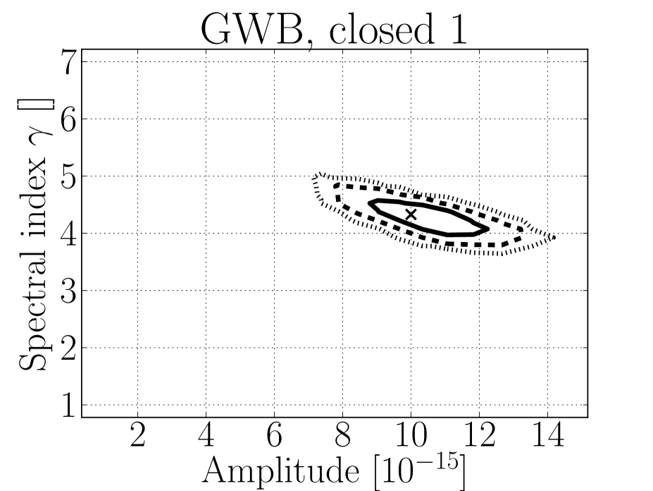
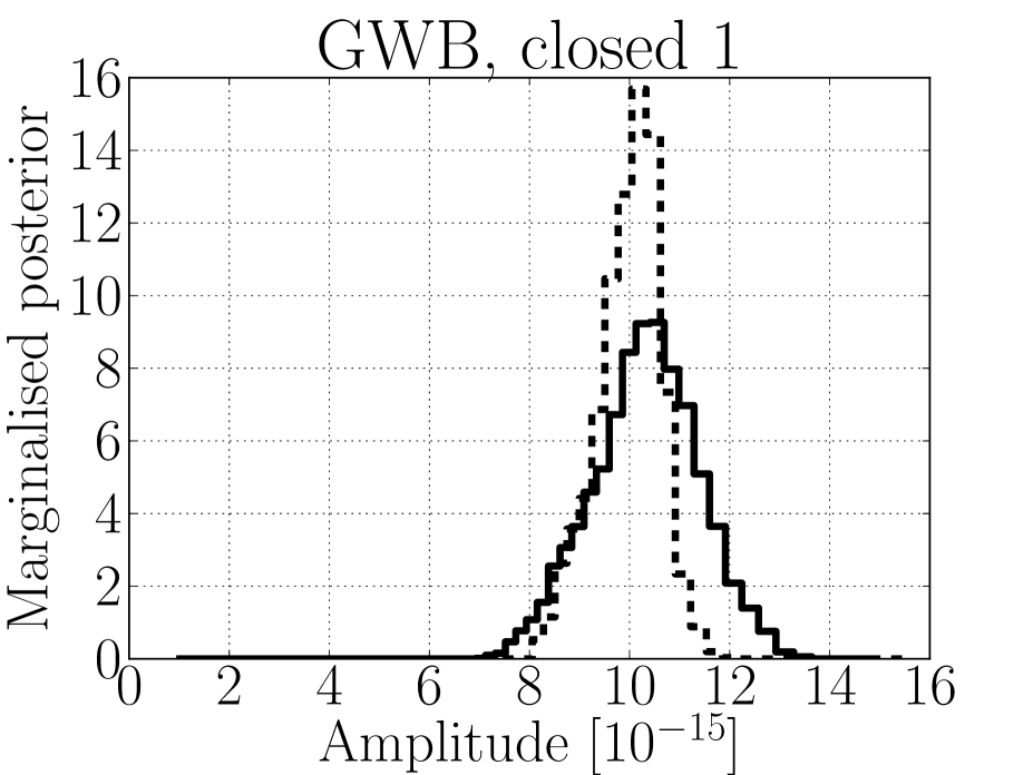
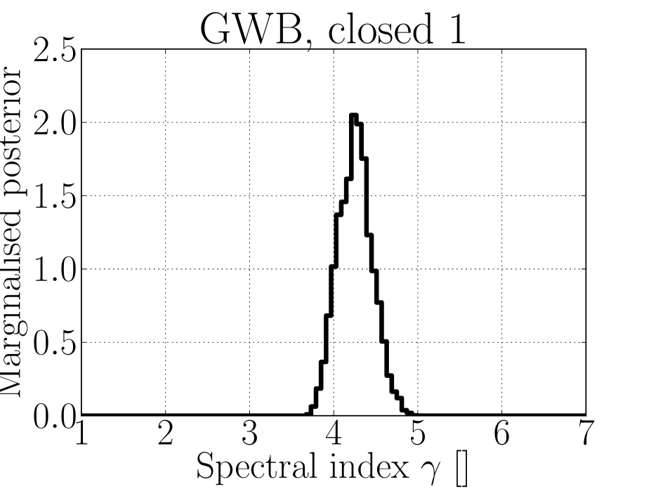
Figure 1: Closed challenge 1, marginalised posterior distributions for a model with $36\times 2+2=74$ free parameters. If we run an MCMC with $\gamma_{\rm GWB}=13/3$ fixed, then we get $h_{c}=10.0\pm 0.64[10^{-15}]$, with a one-sided $2\sigma$ upper-limit of $h_{c}\leq 10.98[10^{-15}]$

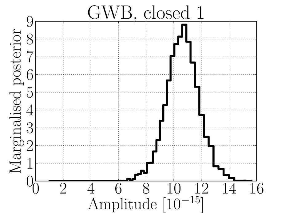
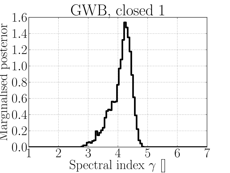
Figure 2: Closed challenge 1, marginalised posterior distributions for a model with $4$ free parameters, where all the pulsars are assumed to have an equal red noise contribution.

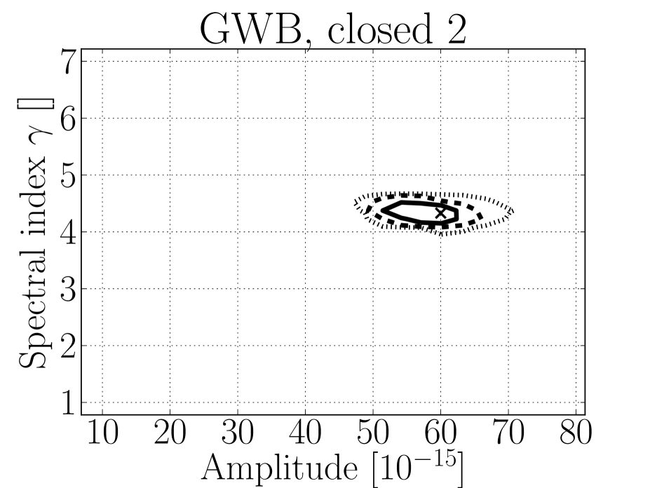
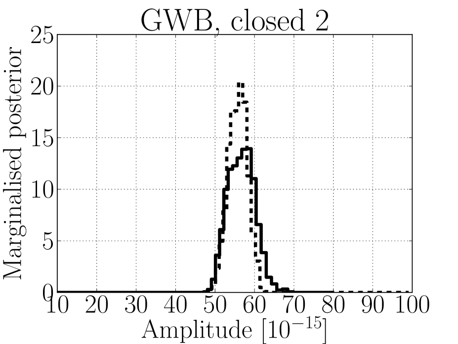
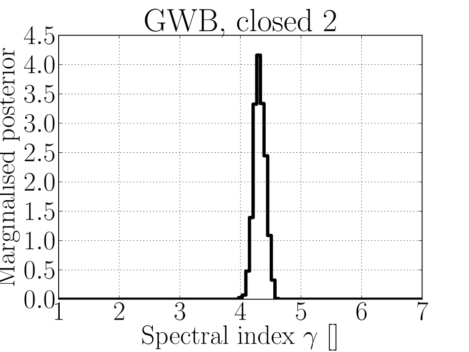
Figure 3: Closed challenge 2, marginalised posterior distributions for a model with $36\times 2+2=74$ free parameters. If we run an MCMC with $\gamma_{\rm GWB}=13/3$ fixed, then we get $h_{c}=56.3\pm 2.42[10^{-15}]$, with a one-sided $2\sigma$ upper-limit of $h_{c}\leq 60.29[10^{-15}]$

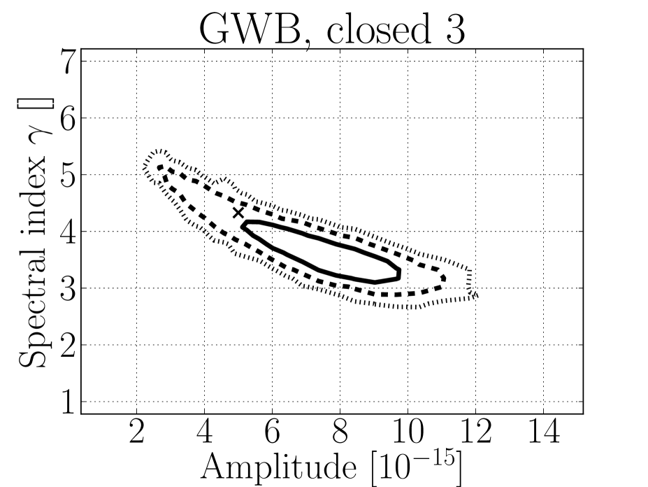
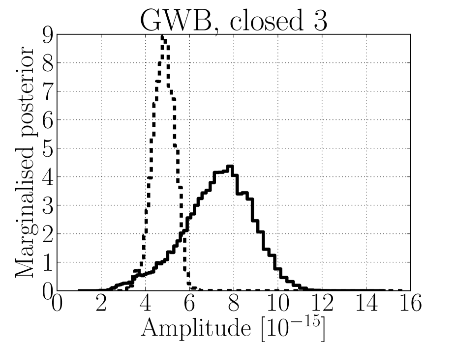
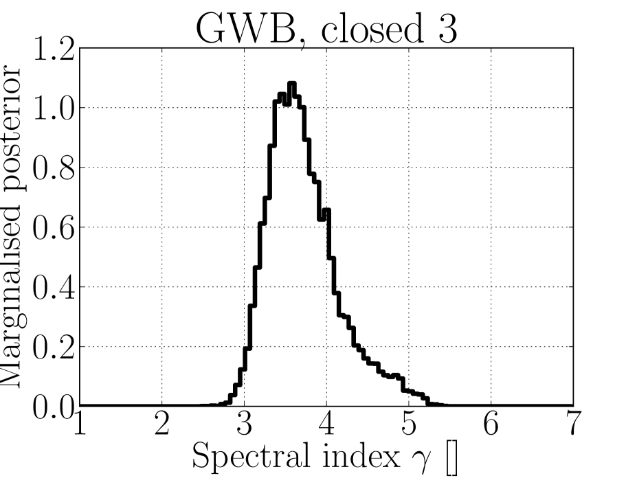
Figure 4: Closed challenge 3, marginalised posterior distributions for a model with $36\times 2+2=74$ free parameters. If we run an MCMC with $\gamma_{\rm GWB}=13/3$ fixed, then we get $h_{c}=4.83\pm 0.50[10^{-15}]$, with a one-sided $2\sigma$ upper-limit of $h_{c}\leq 5.65[10^{-15}]$

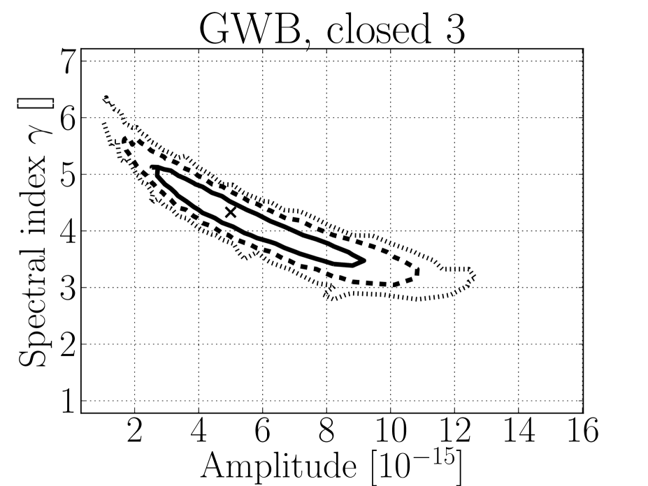
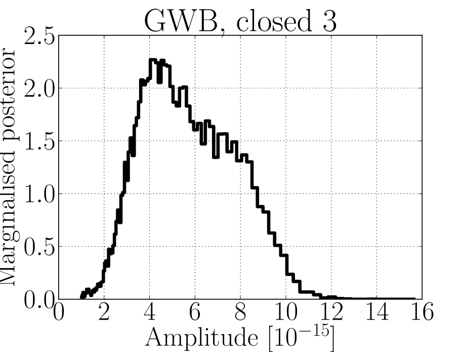
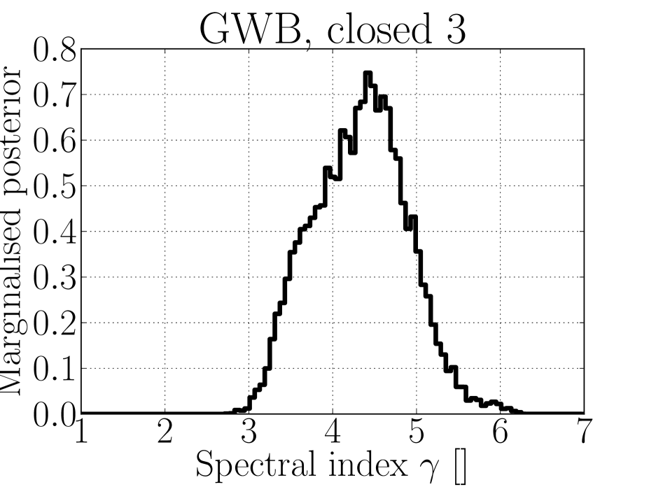
Figure 5: Closed challenge 3, marginalised posterior distributions for a model with $4$ free parameters, where all the pulsars are assumed to have an equal red noise contribution.

References

- Christen & Fox, (2010) Christen, J. A., & Fox, C. 2010. A general purpose sampling algorithm for continuous distributions (the t-walk). Bayesian Anal., 5(Nov.), 263–281.
- Edwards et al., (2006) Edwards, R. T., Hobbs, G. B., & Manchester, R. N. 2006. TEMPO2, a new pulsar timing package - II. The timing model and precision estimates. MNRAS, 372(Nov.), 1549–1574.
- Feroz et al., (2009) Feroz, F., Hobson, M. P., & Bridges, M. 2009. MULTINEST: an efficient and robust Bayesian inference tool for cosmology and particle physics. MNRAS, 398(Oct.), 1601–1614.
- Foreman-Mackey et al., (2012) Foreman-Mackey, D., Hogg, D. W., Lang, D., & Goodman, J. 2012. emcee: The MCMC Hammer. ArXiv e-prints, Feb.
- Hellings & Downs, (1983) Hellings, R.W., & Downs, G.S. 1983. Upper limits on the isotropic gravitational radiation background from pulsar timing analysis. ApJ, 265, L39–L42.
- Hobbs et al., (2006) Hobbs, G. B., Edwards, R. T., & Manchester, R. N. 2006. TEMPO2, a new pulsar-timing package - I. An overview. MNRAS, 369(June), 655–672.
- Press et al., (1992) Press, William, Teukolsky, Saul, Vetterling, William, & Flannery, Brian. 1992. Numerical Recipes in C. 2nd edn. Cambridge, UK: Cambridge University Press.
- Roberts et al., (1997) Roberts, G.O., Gelman, A., & Gilks, W.R. 1997. Weak convergence and optimal scaling of random walk Metropolis algorithms. Ann. of Appl. Prob., 7(1), 110–120.
- Taylor et al., (2012) Taylor, S. R., Gair, J. R., & Lentati, L. 2012. Weighing The Evidence For A Gravitational-Wave Background In The First International Pulsar Timing Array Data Challenge. ArXiv e-prints, Oct.
- van Haasteren, (2012) van Haasteren, R. 2012. Accelerating pulsar timing data analysis. ArXiv e-prints, Oct.
- van Haasteren & Levin, (2010) van Haasteren, R., & Levin, Y. 2010. Gravitational-wave memory and pulsar timing arrays. MNRAS, 401(Feb.), 2372–2378.
- van Haasteren & Levin, (2012) van Haasteren, R., & Levin, Y. 2012. Understanding and analysing time-correlated stochastic signals in pulsar timing. ArXiv e-prints, Feb.
- van Haasteren et al., (2009) van Haasteren, R., Levin, Y., McDonald, P., & Lu, T. 2009. On measuring the gravitational-wave background using Pulsar Timing Arrays. MNRAS, 395(May), 1005–1014.
- van Haasteren et al., (2011) van Haasteren, R., Levin, Y., Janssen, G. H., Lazaridis, K., Kramer, M., Stappers, B. W., Desvignes, G., Purver, M. B., & Lyne, A. G. 2011. Placing limits on the stochastic gravitational-wave background using European Pulsar Timing Array data. MNRAS, 414(July), 3117–3128.