Analytical formulas, general properties and calculation of transport coefficients in the hadron gas: shear and bulk viscosities.

Abstract

Elaborated calculations of the shear and the bulk viscosities in the hadron gas, using the ultrarelativistic quantum molecular dynamics (UrQMD) model cross sections, are made. These cross sections are analyzed and improved. A special treatment of the resonances is implemented additionally. All this allows for better hydrodynamical description of the experimental data. The previously considered approximation of one constant cross section for all hadrons is justified. It’s found that the bulk viscosity of the hadron gas is much larger than the bulk viscosity of the pion gas while the shear viscosity is found to be less sensitive to the hadronic mass spectrum. The maximum of the bulk viscosity of the hadron gas is expected to be approximately in the temperature range ${T=150-190~{}MeV}$ with zero chemical potentials. This range covers the critical temperature values found from lattice calculations. We comment on some important aspects of calculations of the bulk viscosity, which were not taken into account or were not analyzed well previously. Doing this, a generalized Chapman-Enskog procedure, taking into account deviations from the chemical equilibrium, is outlined. Some general properties, features, the physical meaning of the bulk viscosity and some other comments on the deviations from the chemical equilibrium supplement this discussion. Analytical closed-form expressions for the transport coefficients and some related quantities within a quite large class of cross sections can be obtained. Some examples are explicitly considered. Comparisons with some previous calculations of the viscosities in the hadron gas and the pion gas are done.

I Introduction

The bulk and the shear viscosity coefficients are transport coefficients which enter in the hydrodynamic equations, and thus are important for studying of nonequilibrium evolution of any thermodynamic system.

There are two more additional reasons to study the shear viscosity. The first one is the experimentally observed minimum of the ratio of the shear viscosity to the entropy density $\eta/s$ near the liquid-gas phase transition for different substances, which may help in studying of the quantum chromodynamics phase diagram and finding of the location of the critical point Csernai:2006zz ; lacey . Such a minimum was observed in theoretical results in several models, see e. g. chakkap ; Dobado:2009ek . For a counterexample see Chen:2010vf and references therein. The second reason is the calculation of the $\eta/s$ in strongly interacting systems, preferably real ones, to compare physical inputs which provide small values of the $\eta/s$. The conjectured lowest bound $\eta/s=\frac{1}{4\pi}$ adscftbound was violated with different counterexamples. For some reasonable ones see Buchel:2008vz ; Sinha:2009ev . Also see the recent review Cremonini:2011iq . The bulk viscosity, being very sensitive to violation of the equation of state and being connected with fluctuations through the fluctuation-dissipation theorem Callen:1951vq , can have a maximum near a phase transition Kharzeev:2007wb ; Karsch:2007jc ; chakkap ; Dobado:2012zf . In chakkap and Dobado:2012zf sharp maxima were observed in the bulk viscosity $\xi$ and the ratio $\xi/s$ in the linear $\sigma$-model for the vacuum $\sigma$ mass $900~{}MeV$. Decreasing the vacuum $\sigma$ mass the maximum eventually disappears. Any maximum of the $\xi/s$ was not observed in the large-N limit of the linear $\sigma$-model in the Dobado:2012zf . Any maximum of the $\xi$ was not observed in the large-N limit of the ${1+1}$-dimensional Gross-Neveu model FernandezFraile:2010gu (see also Sec. II for comments).

Whether one uses the Kubo formula or the Boltzmann equation one faces nearly the same integral equation for the transport coefficients jeon ; jeonyaffe ; Arnold:2002zm . The preferable way to solve it is the variational (or Ritz) method. Due to its complexity the relaxation time approximation is used often in the framework of the Boltzmann equation. Though this approximation is inaccurate, does not allow to control precision of approximation and can potentially lead to large deviations. The main difficulty in the variational method is in calculation of collision integrals. To calculate any transport coefficient in the lowest order approximation in a mixture with a very large number of components $N^{\prime}$ (like in the hadron gas) one would need to calculate roughly ${N^{\prime}}^{2}$ 12-dimensional integrals if only the elastic collisions are considered. Fortunately, it’s possible to simplify these integrals considerably and perform these calculations in a reasonable time.

This paper contains calculations of the shear and the bulk viscosity coefficients for the hadron gas using the (corrected, see Sec. III) UrQMD cross sections. The calculations are done in the framework of the Boltzmann equation with the classical Maxwell-Boltzmann statistics, without medium effects and with the ideal gas equation of state. The Maxwell-Boltzmann statistics approximation allows one to obtain some relatively simple analytical closed-form expressions. Originally the calculations in the same approximations for the hadron gas but with one constant cross section for all hadrons were done in Moroz:2011vn . The deviations in the worst cases are relatively small. In that paper some analytical formulas of the viscosities for 1-, 2- (explicitly) and N-component (up to solution of the matrix equation) gases with constant cross sections were obtained. Analogical formulas can be written down for quite a large class of non-constant cross sections, in particular, for the ones which appear in the chiral perturbation theory. The final expressions may become somewhat more cumbersome; anyway this is better than numerical integration at least in the speed of the computation. Explicit formulas for the viscosities with the elastic pion-pion isospin averaged cross section and somewhat more general one are obtained in the present paper. The results of the Moroz:2011vn are partially reproduced in the present paper, improving the text and adding more detailed explanations. The presented calculations can be considered as quite precise ones at low temperatures where the elastic collisions dominate and the equation of state is close to the ideal gas equation of state. At higher temperatures the calculations with the total cross section are expected to give the qualitative description.

For comparison the calculations of the viscosities are performed for the pion gas (throughout the paper the chemical potentials are equal to zero if else is not stated). The results are relatively close to the results in prakash ; davesne . There the calculations are made in the same approximations except for the davesne , where the Bose-Einstein statistics is used instead of the Maxwell-Boltzmann one. The discrepancies from the used classical statistics are not large at zero chemical potential and become larger as the chemical potential grows (see Sec. IV for the errors and comments). The comparison is made with the results of the prakash , see fig. 1. The discrepancies up to a factor of $3.5$ for the bulk viscosity and up to a factor of $2.5$ for the shear viscosity come most probably from somewhat different ${\pi\pi}$ elastic plus the quasielastic (through the intermediate $\rho$-resonance) cross section of the prakash (the averaging over the scattering angle is expected to give small errors; see also comments below the formula (128)). The minima of the shear viscosities near ${T=60-70~{}MeV}$ are attributed to the peaks from the $\rho$-resonances in the ${\pi\pi}$ cross sections. It’s not noticeable in the figure for the dash-dotted line. Nonzero values of the bulk viscosities and theirs maxima are solely due to the masses of the pions. The paper prakash implements also the isospin averaged current algebra elastic cross sections. These cross sections can be reproduced in the lowest order in the chiral perturbation theory Scherer:2002tk . They obviously have quite large deviations from the experimental data at high enough energies and wrong $\sqrt{s}$ asymptotic dependence, which can be seen from the comparison of them with the isospin averaged elastic plus the quasielastic experimental cross sections in the prakash . The elastic $\pi\pi$ cross sections are rather close to the constant $5~{}mb$ Bass:1998ca ; Bleicher:1999xi .

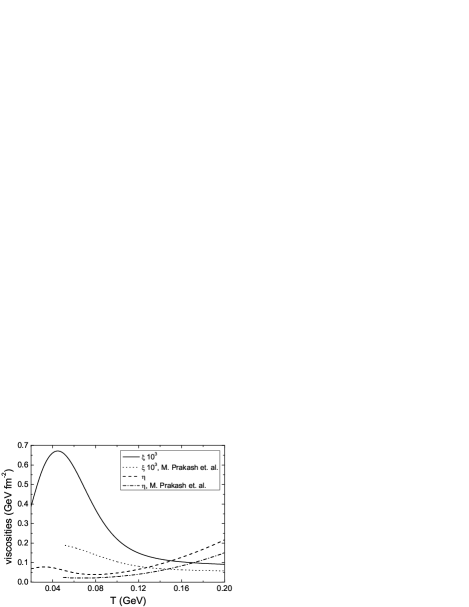
Figure 1: The viscosities of the pion gas as functions of the temperature at zero chemical potentials. The dotted and the dash-dotted lines designate correspondingly the bulk viscosity time $10^{3}$ and the shear viscosity, calculated in the 3-rd order in the prakash . The solid and the dashed lines designate correspondingly the bulk viscosity time $10^{3}$ and the shear viscosity, calculated at the same orders using the (corrected, see Sec. III) UrQMD cross sections.

In several papers the bulk viscosity $\xi$ was calculated for the pion gas, using the chiral perturbation theory (or the unitarized chiral perturbation theory) and some other approaches, with quite large discrepancies between the quantitative results. In fernnicola the calculations were done by the Kubo formula in a rough approximation. There the number-changing ${2\leftrightarrow 4}$ processes were neglected too, and the non-vanishing value of the bulk viscosity is obtained due to a trace anomaly and the pions’ masses. At small temperatures, where the effects of the trace anomaly are small, the magnitude of the bulk viscosity is large in compare to the results of this paper and the prakash ; davesne . For example, at ${T=20~{}MeV}$ (${60~{}MeV}$) it’s larger approximately in 39 (8) times than the bulk viscosity in this paper. The maximal values differ in approximately 24 times. In lumoore the calculations are done in the framework of the Boltzmann equation and have a divergent dependence of the $\xi$ for ${T\rightarrow 0}$ because of remained weak ${2\leftrightarrow 4}$ number-changing processes (at ${T=140~{}MeV}$ the bulk viscosity is nearly 57 times larger than the bulk viscosity calculated in this paper). This dependence should change at low enough temperatures, $T=180~{}MeV$ or higher ones for the pion gas, see Sec. II for explanations. Joining the results of the calculations at low and high temperatures, the function $\xi(T)$ may turn out to be not continuous at the middle temperatures (which is not a physical effect, see Sec. II), and the smooth function $\xi(T)$ is to be obtained through some interpolation. In dobado the bulk viscosity was calculated in the framework of the Boltzmann equation with the ideal gas equation of state and only the elastic collisions taken into account. The Inverse Amplitude Method was used to get the scattering amplitudes of the pions. The quantitative results are close to the results in this paper (discrepancies up to a factor of $2.7$). In chenwang the calculations are done in the framework of the Boltzmann equation for the massless pions. There the bulk viscosity increases rapidly so that the ratio $\xi/s$ increases with the temperature.

Calculations of the shear viscosity in the hadron gas with a large number of components were done in Gorenstein:2007mw , using some approximate phenomenological formula, and in toneev , using the relaxation time approximation. These results are in good agreement with the calculations of this paper. Hence, as long as the ratio $\xi/\eta$ calculated in the toneev for the free massive pion gas is $8-58$ times larger (in the temperature range $0.02~{}GeV<T<0.14~{}GeV$ with the deviations growing as the temperature decreases) than the one calculated in this paper, one can suspect that the difference comes from the bulk viscosity because of the used relaxation time approximation and likely not conserved particle numbers at low temperatures, provided that the SHMC model’s cross sections, used in the toneev , don’t have large deviations from the UrQMD cross sections or the experimental data, which seems to be the case. Also note that the results in the toneev for the free particles and the SHMC model don’t differ very much. These facts may explain why the $\xi/s$ of the hadron gas in the toneev is $3.65-11.3$ times larger (in the temperature range $0.1~{}GeV<T<0.18~{}GeV$) than the $\xi/s$ calculated in this paper. At the low temperature ${T=100~{}MeV}$ and the vanishing chemical potentials it is 11.3 times more (at the same temperature the factor is 8.2 for the case of the pion gas). In nhngr the calculation of the bulk viscosity is done for the hadron gas (with an excluded-volume equation of state) with the masses less than $2~{}GeV$ using some special formula, obtained though some ansatz Kharzeev:2007wb . Its quantitative accuracy has not been clarified. The ratio $\xi/s$ in the nhngr deviates from the $\xi/s$ of this paper up to a factor of 1.8 in the temperature range $0.14~{}GeV<T<0.18~{}GeV$ and is different on $4\%$ at $T=0.14~{}GeV$.

Also the shear viscosity has been calculated using the Kubo formula (or the Green-Kubo formula) in a gas of mesons and their resonances Muronga:2003tb . There the UrQMD simulations are performed to calculate the energy-momentum tensor, used in the calculations by the Kubo formula. The $\eta$ in the Muronga:2003tb is $1.14-1.77$ times smaller then the $\eta$ for the hadron gas in this paper. At $T=0.15~{}GeV$ it is $1.77$ times smaller. In Muroya:2004pu similar calculations, using the URASiMA event generator, are done for the shear viscosity with close results.

The structure of the paper is the following. A misleading viewpoint on the bulk viscosity, connected with the inelastic processes, is commented on in Sec. II together with some properties, features and physical meaning of the bulk viscosity. In that section some questions concerning the deviations from the chemical equilibrium are addressed too. Sec. III contains some comments on the constant cross sections, which are used in approximating calculations, and some other general comments on cross sections. Also it contains a description of the UrQMD cross sections, which are used in the main calculations, together with their analysis, corrections and the consequences of the corrections for the freeze-out temperatures. The applicability of the used through the paper approximations is discussed in Sec. IV. The system of the Boltzmann equations, its solution and formal expressions of the transport coefficients can be found in Sec. V. The numerical calculations for the hadron gas are presented in Sec. VI. In Sec. VII.1 analytical results for the single-component gas are presented. In particular, an analytical expression for the first order single-component shear viscosity coefficient with constant cross section, found before in anderson , is corrected while the bulk viscosity coefficient remains the same. The nonequilibrium distribution function in the same approximation is written down. Also the viscosities with some non-constant cross sections are written down. Some analytical results for the binary mixture with constant cross sections are considered in Sec. VII.2. Integrals of source terms needed for the calculation of the transport coefficients can be found in Appendix A. The general entropy density formula can be found in Appendix B. It is used in the numerical calculations for the hadron gas. Transformations of collision brackets, being the 12-dimensional integrals which enter in the viscosities, and some analytical formulas for them can be found in Appendix C. The closed-form expressions for collision rates, mean free paths and mean free times are included in Appendix D.

II Some features and properties of the bulk viscosity

First, it should be reminded that the transport coefficients are defined as coefficients next to their gradients in the formal expansion of the energy-momentum tensor and the charge density flows over the gradients of the thermodynamic functions or the flow velocity (see e. g. landau6 , Section 136). The Kubo formulas are not definitions of the transport coefficients, as one might think. They may introduce some assumptions. In particular, the Kubo formulas in the form as in the jeon have zero frequency and zero momentum limits, which neglect finite size and finite time effects. Zero momentum limit implies the thermodynamical limit. This limit is needed to avoid possible nonphysical contributions from inappropriate choice of a current and an ensemble Kadanoff . The Kubo formulas in the form as in Muroya:2004pu ; Kubo suppose thermal equilibrium in the initial moment of time $t=-\infty$. So that any infinite space-time scale cannot be connected with the transport coefficients by their definitions.

The Boltzmann equations will be used in what follows. In the case of the elastic collisions they can be derived from the Liouville equation in the approximations $n_{k}r_{kl}^{3}\ll 1$ ($r_{kl}$ is the effective radius of two particle interactions between the particles of the species $k$ and $l$) that is for rarified gases with short-range interactions. Also the linear integral equations for the viscosities and other transport coefficients, derivable from the Boltzmann equation, can be obtained (with some corrections) from the perturbative calculations for quantum field theories at finite temperature (including the inelastic processes) using the Kubo formulas jeon ; Gagnon:2006hi ; Gagnon:2007qt , which justifies application of the Boltzmann equation when the inelastic processes are present.

The bulk viscosity can reveal itself only when there is a nonzero divergence of the flow velocity. This nonequilibrium perturbation should not be confused with another possible independent perturbation (as was done in several papers, some of which are mentioned below; the roots of the misleading viewpoint, perhaps, can be found in landau6 , Section 81). Namely, this is the homogeneous perturbation. It can be both the chemical and the kinetic one. Then it can be generalized and made dependent on the coordinate. It just should not be proportional to any gradient. Then the constraints of the local conservation laws should be imposed on these perturbations. The perturbations for the particle numbers should be such that don’t violate conservation of all charges. Considering the case of homogeneous chemical perturbation in a gas with fixed volume, one concludes that the temperature should change with time, being some energy per particle. So that energy conservation should be obtained varying the temperature. Adding an infinitesimal correction to the temperature one gets a perturbation of the form $Cp_{k}^{\mu}U_{\mu}$. Such perturbations don’t contribute to all collision integrals. To describe purely chemical perturbations they have to be chosen in the form of the momentum-independent terms (except for the $Cp_{k}^{\mu}U_{\mu}$ terms), otherwise there will be contributions from the elastic collision integrals. Such perturbations can be considered as chemical potentials-like ones (being small, one can expand the distribution functions over them and get these momentum-independent terms) with the arguments for maximization of the entropy. To find the evolution of these terms they should be separated. Let’s write this in some formulas. Multicomponent gas distribution functions with the leading perturbations can be represented in the form (detailed definitions can be found in Sec. V.1)

$$f_{k}=f_{k}^{(0)}(1+\tilde{\varphi}_{k})(1+\varphi_{k})\approx f_{k}^{(0)}(1+\tilde{\varphi}_{k}+\varphi_{k}),\quad|\tilde{\varphi}_{k}|\ll 1,\quad|\varphi_{k}|\ll 1,$$ (1)

where $\varphi_{k}$ are the perturbation due to the gradients and $\tilde{\varphi}_{k}$ are the chemical perturbations. Following steps of Sec. V.1, one can get the following linearized equations from the Boltzmann equations:

$$p_{k}^{\mu}(U_{\mu}D+\nabla_{\mu})f^{(0)}_{k}+f^{(0)}_{k}p_{k}^{\mu}(U_{\mu}D+\nabla_{\mu})\tilde{\varphi}_{k}\approx-f_{k}^{(0)}\mathcal{L}_{k}[\varphi_{k}]-f_{k}^{(0)}\mathcal{L}_{k}^{inel}[\tilde{\varphi}_{k}],$$ (2)

where $\mathcal{L}_{k}$ and $\mathcal{L}_{k}^{inel}$ is the sum of the linearized collision integrals (divided on the $-f_{k}^{(0)}$) of all the processes and of the inelastic processes correspondingly. The 2-nd order gradients and the squared 1-st order gradients are neglected in the l. h. s. because they are of the next order and should be cancelled in the next iteration by the next corrections to the distribution functions. Also the smallness of the $\tilde{\varphi}_{k}$ is used. If the spatial covariant gradients $\nabla_{\mu}\tilde{\varphi}_{k}(t=0)$ (at the initial moment of time) are of the same order as the gradients of the thermodynamic functions or the flow velocity, then the $\nabla_{\mu}\tilde{\varphi}_{k}$ terms in the l. h. s. should be retained. The covariant temporal derivatives $D\tilde{\varphi}_{k}$ are needed to describe the temporal evolution of the $\tilde{\varphi}_{k}$. Then the equations (2) can be split onto the separate equations for the $\tilde{\varphi}_{k}$ and the $\varphi_{k}$

$$p_{k}^{\mu}U_{\mu}D\tilde{\varphi}_{k}+p_{k}^{\mu}\nabla_{\mu}\tilde{\varphi}_{k}\approx-\mathcal{L}_{k}^{inel}[\tilde{\varphi}_{k}],$$ (3)

$$p_{k}^{\mu}U_{\mu}Df^{(0)}_{k}+p_{k}^{\mu}\nabla_{\mu}f^{(0)}_{k}\approx-f_{k}^{(0)}\mathcal{L}_{k}[\varphi_{k}].$$ (4)

The equations (2) can be split within the framework of the perturbation theory over the gradients. Let’s consider also the condition $\varphi_{k}\ll\tilde{\varphi}_{k}$ in the (1). Then neglecting the $\varphi_{k}$ in the (1) and repeating the steps of Sec. V.1, one can get the following linearized equations:

$$p_{k}^{\mu}U_{\mu}D\tilde{\varphi}_{k}\approx-\mathcal{L}_{k}^{inel}[\tilde{\varphi}_{k}].$$ (5)

The equations (5) are precise in the homogeneous case (the approximation is only from the linearization). The 1-st order gradients and the $\nabla_{\mu}\tilde{\varphi}_{k}$ are neglected. Then using the (5) and the (2), one can get

$$(p_{k}^{\mu}U_{\mu}D+p_{k}^{\mu}\nabla_{\mu})f^{(0)}_{k}+f^{(0)}_{k}p_{k}^{\mu}\nabla_{\mu}\tilde{\varphi}_{k}\approx-f_{k}^{(0)}\mathcal{L}_{k}[\varphi_{k}].$$ (6)

Solving the system of equations (5) in the local rest frame, one gets the leading exponential fading dependencies on time (in a covariant form this should be an explicit space-time dependence). Such dependencies were obtained in some previous studies, see e. g. Matsui:1985eu ; Song:1996ik . The equations (6) are different from the ones obtained from the common Chapman-Enskog procedure (see e. g. groot , Chap. V) because of the $\nabla_{\mu}\tilde{\varphi}_{k}$ terms. The contributions from the small chemical perturbations can be neglected in the considered order in the transport coefficients because they are multiplied on the 1-st order gradients. The $\nabla_{\mu}\tilde{\varphi}_{k}$ terms can be cancelled, introducing terms proportional to the $\nabla_{\mu}\tilde{\varphi}_{k}(t=0)$ into the $\varphi_{k}$ terms. If the spatial distributions of the $\tilde{\varphi}_{k}(t=0)$ are such that $\nabla_{\mu}\tilde{\varphi}_{k}(t=0)$ are of the 2-nd or a higher order, then the $\nabla_{\mu}\tilde{\varphi}_{k}$ can be neglected. This assumption or approximation is used in the calculations of this paper. In the linear response theory one can also introduce independent small chemical perturbations with the same conclusions for the 1-st order transport coefficients and find evolution of the perturbations with time.

Note that the deviation from the chemical equilibrium itself is not necessarily a source of the bulk viscosity, as is stated in Paech:2006st . If the bulk viscosity is not equal to zero only because of the particles’ masses and they are tended to zero, the bulk viscosity source term and the bulk viscosity tend to zero even if there are inelastic processes (see the end of Sec. V.1). In the Paech:2006st the independent chemical perturbations and the perturbations due to the gradients were just connected through the perturbations of particle numbers, and the bulk viscosity became proportional to the chemical relaxation time. Formally infinite chemical relaxation time doesn’t imply any divergencies in the chemical perturbations $\tilde{\varphi}_{k}$, but rather approximation of conserved particle numbers. Note that the dependence on the strength of the inelastic processes is different for the chemical perturbations and the perturbations due to the gradients. Increasing the strength of the inelastic processes the chemical relaxation time decreases. And the gradients’ relaxation time increases, because the transport coefficients, at least in rarified gases with short-range interactions, roughly speaking, are inversely proportional to the integrated cross sections (in an ideal liquid the gradients’ relaxation time is infinite). What happens with the bulk viscosity if the inelastic processes become weaker is discussed below.

Making the inelastic processes weaker in compare to the elastic ones, the bulk viscosity eventually gets a formal dominant contribution from them because of the approximate zero mode(s) jeon , connected with possible conservation of particle number(s). As long as it’s clear that the bulk viscosity is not responsible for the chemical equilibration, it’s also clear that there may be the approximation of conserved particle numbers if the momentum spectrum, as well as the gradients, can relax by means of only the elastic collisions (which is usually the case) and the elastic processes make a dominant contribution to the collision rates. The question is only at what concrete temperature does this approximation sets in. Let’s make an illustrative example of what nonphysical contributions one can get from formally remained weak inelastic processes. Consider infinitely weak inelastic processes and the perturbation of the flow velocity such that the energy-momentum tensor gets a sizable contribution from the bulk viscosity term, not large in compare to the pressure (cf. (20), (27)) to remain the perturbation theory applicable. Then it’s obvious that this contribution is not physical because it is created by the practically absent processes and the infinitesimal perturbation of the flow velocity. Instead, this system is practically described by the equilibrium thermodynamic functions. This also answers positively the question whether the thermodynamic chemical potential can be introduced for approximately conserved particle number in principle. As far as the author knows, the first correct comment (albeit somewhat inaccurate) on this issue can be found in the jeonyaffe . However, note that in fact there is no divergent mean free paths, corresponding to the inelastic processes (IMFP) in this case. They are cut by the mean free paths, corresponding to the elastic processes (and the overall collision rate have the dominant contribution from the elastic collisions). So that it may be not necessary for the chemical relaxation time to be much larger than any relevant time scale (like the gradients relaxation time or the time of existence of the thermal part of the system) to switch off the inelastic processes. That’s why a criterion based on comparison of collision rates of elastic and inelastic processes can be considered to switch off the inelastic processes. Such a comparison is done in the UrQMD studies of the hadron gas in Bleicher:2002dm (see Sec. IV for farther discussions). According to Goity , the chemical relaxation time of the $2\leftrightarrow 4$ processes in the pion gas is much larger than the thermal relaxation time. And e. g. at $T=180~{}MeV$ the chemical relaxation time is equal to $40~{}fm$, which is larger than the typical lifetime of the thermal part of the expanding fireball (see e. g. Bleicher:2002dm ). So that it’s the inelastic $2\leftrightarrow 4$ processes which should be neglected in the pion gas at $T=180~{}MeV$ or even higher temperatures, which wasn’t done in the lumoore . To show importance of the gradients relaxation time, let’s consider the following possible case. Let’s consider the only perturbation - propagating sound wave, perturbed in a point. It’s possible for the IMFP to be much larger than the gradients relaxation size (on which the wave can be considered as damped) and be much smaller than the system’s size at the same time. Then, the bulk viscosity cannot be defined by the IMFP in this case, because it enters in the sound attenuation constant. Thus, the gradients relaxation size and time are cutting parameters. Note that they exists even in infinite systems considered during infinite time interval.

The bulk viscosity source terms increases substantially if particle numbers are not conserved (cf. (120), (121); in mixtures these particle numbers should also be not small). This reflects additional fluctuations from not conserved particle numbers. Though the inelastic processes have to be effective enough to consider the approximation of not conserved particle numbers. Perhaps, the point at which the bulk viscosities in the different approximations cross can provide a criterion for switching on/off the inelastic processes. If this is not so, then one would have to make some interpolation in the intermediate region. Note that e. g. in the calculations by the Kubo formulas through the direct calculations of the energy-momentum tensor as in the Muronga:2003tb it’s not needed to use the approximation of conserved or not conserved particle numbers (which defines the number of independent thermodynamic chemical potentials, through which the chemical potentials of all particles are expressed, cf. (18)). There the energy-momentum tensor should be a smooth function of time and the thermodynamic functions as long as the inelastic processes fade smoothly. Then the bulk viscosity should be a smooth function of the temperature and particles’ chemical potentials regardless of the number of the independent chemical potentials.

In the Arnold:2006fz a bottleneck for the relaxation to equilibrium characterized by the bulk viscosity due to the weakest processes’ rates is assumed. Instead, there are rather dominant contributions from some test-functions (as is commented in the footnote 13), which should not be specially treated though, except for the ones which are the approximate zero modes making a dominant contribution. A similar dominance is present also in other transport coefficients, in particular, when there is only one type of processes. Although in QCD at high enough temperatures the equilibrium $2\leftrightarrow 2$ elastic collisions rate is parametrically the largest one, $O(\alpha_{s}T)$, because of cancellations the momentum transfer takes place with the rate $O(\alpha_{s}^{2}\ln(1/\alpha_{s})T)$, which is parametrically smaller than the particle number change rate $O(\alpha_{s}^{3/2}T)$ from the effective ”$1\leftrightarrow 2$” processes. This provides an example when the equilibrium collision rates may differ substantially from the relevant collision rates. The ”$1\leftrightarrow 2$” processes provide small chemical relaxation time in compare to the thermal relaxation time, which justifies the approximation of not conserved particle numbers and the enhancement of the bulk viscosity from the source terms at least at small enough $\alpha_{s}$, whereas the contributions to the bulk viscosity from the collision integrals of the ”$1\leftrightarrow 2$” processes are suppressed at small enough $\alpha_{s}$ (the inelastic $2\leftrightarrow 2$ processes are not suppressed, but they are of the order $O(\alpha_{s}^{2}\ln(1/\alpha_{s})T)$). To avoid misunderstanding it may be mentioned that taking the total collision rate of the ”$1\leftrightarrow 2$” processes as formally infinite by taking the corresponding matrix elements as formally infinite ones, one gets zero bulk viscosity and zero mean free paths as long as both the gluons and quarks take part in these processes (see also footnote 24).

In the case of a ${1+1}$-dimensional single-component gas the elastic collisions cannot result in the relaxation of the momentum spectra and, hence, cannot stimulate the system to evolute towards equilibrium. As a result, the exponentially divergent bulk viscosity was obtained in the paper FernandezFraile:2010gu . Considering again the example about the infinitely small perturbation of the flow velocity and assuming also a finite size of the system, it’s again obvious that the weak inelastic processes may make nonphysical contributions (in this case the mean free path is formally cut by the system’s size). If this is the case, then the hydrodynamical description becomes inapplicable, and might use simulations of particles’ collisions or the Boltzmann equations in the approximation without collisions (on a time scale much smaller than the chemical relaxation time). If the ${1+1}$-dimensional description is only an approximate one (that is with small angle elastic scatterings in higher dimensions), the relaxation of the momentum spectrum by the elastic collisions should be considered. And if a $1+1$-dimensional gas has at least two components with different masses, then a nontrivial momentum exchange in the elastic collisions is possible. This results in the possibility of the relaxation of the momentum spectra by only the elastic collisions Cubero .

Let’s summarize this section with formulation of the physical meaning of the bulk viscosity. The bulk viscosity reflects deviation of the value of the pressure from its local equilibrium value (as can be seen from the (27)), appearing when the system expands/compresses, because of the delay in the equilibration. The bulk viscosity is not responsible for the restoration of the chemical or the kinetic equilibria - it’s responsible for the relaxation of the divergence of the flow velocity. If there are inelastic processes, then the particle numbers also get nonequilibrium contributions (cf. (14), (37), (68)) such that the charge is conserved locally (cf. (74)). Though these contributions together with the contribution to the pressure may become nonphysical because of the approximate zero modes (if such ones appear in the calculations). The magnitude of the bulk viscosity changes from theory to theory. Under some quite general assumptions a nonzero value of the bulk viscosity can be connected with violation of the scale invariance due to a nonzero value of the energy-momentum tensor Coleman:1970je ; Callan:1970ze . Of course, the beta function can contribute to the energy-momentum tensor and the bulk viscosity too jeon .

III The hard core interaction model and the UrQMD cross sections

In a non-relativistic classical theory of particle interactions there is a widespread model, used in approximate calculations, called the hard core repulsion model or the model of hard spheres with some radius $r$. For its applications to the high-energy nuclear collisions see Gorenstein:2007mw and references therein. The differential scattering cross section for this model can be inferred from the problem of scattering of point particle on the spherical potential ${U(r)=\infty}$ if ${r\leq a}$ and ${U(r)=0}$ if ${r>a}$ landau1 . In this model the differential cross section is equal to $a^{2}/4$. To apply this result to the gas of hard spheres with the radius $r$ one can notice that the scattering of any two spheres can be considered as the scattering of the point particle on the sphere of the radius $2r$, so that one should take ${a=2r}$. The total cross section $\sigma_{tot}$ is obtained after integration over the angles of the $r^{2}d\Omega$ which results in the $\sigma_{tot}=4\pi r^{2}$. For collisions of hard spheres of different radiuses one should take ${a=r_{k}+r_{l}}$ or replace the $r$ on the $\frac{r_{k}+r_{l}}{2}$:

$$\sigma_{tot,kl}=\pi(r_{k}+r_{l})^{2}.$$ (7)

The relativistic generalization of this model is the constant (not dependent on the scattering energy and angle) differential cross sections model.

The hard spheres model is classical, and connection of its cross sections to cross sections, calculated in any quantum theory, is needed. For particles, having a spin, the differential cross sections averaged over the initial spin states and summed over the final ones will be used. If colliding particles are identical and their differential cross section is integrated over the momentums (or the spatial angle to get the total cross section) then it should be multiplied on the factor $\frac{1}{2}$ to cancel double counting of the momentum states. These factors are exactly the factors $\gamma_{kl}$ next to the collision integrals in the Boltzmann equations (30). The differential cross sections times these factors will be called the classical differential cross sections.

The UrQMD cross sections are used in the numerical calculations of Sec. VI. These cross sections are described in Bass:1998ca ; Bleicher:1999xi . More details can be found in the UrQMD program codes. Below there is some description mainly of what is different or new.

The UrQMD cross sections are averaged over the initial spin states and summed over the final ones. As long as the UrQMD cross sections are total ones (integrated over the scattering angle), the factors $\gamma_{kl}$ are already absorbed into them (in what follows only such cross sections will be considered in this section tacitly). Dividing them on the $4\pi$, one gets the classical differential cross sections, averaged over the scattering angle.

The UrQMD codes (version 1.3) were modified to get accurately tabulated (with a step of ${25~{}MeV}$) cross sections. Resonances’ masses and widths (they are tuned in their uncertainty regions to describe the experimental data better), used in the UrQMD codes, have somewhat different values than the ones in the Bass:1998ca . Influence of variation of these parameters was studied in Gerhard:2012fj . The UrQMD codes implement somewhat different averaging of the c. m. momentums over the resonances’ masses than in the papers Bass:1998ca ; Bleicher:1999xi . It was found that using the resonance dominating cross sections from the papers Bass:1998ca ; Bleicher:1999xi some of these cross sections could have a large rise at small c. m. momentums if constant widths are used in the calculations of the averaged c. m. momentums in the energy dependent widths. So that one should be aware of this fact. The UrQMD codes have a low energy cut-off at ${\sqrt{s}\sim m_{k}+m_{l}+0.01~{}GeV}$ (and a similar one over the c. m. momentum if triggered) for the resonance dominating cross sections, and no large low energy rise was found there.

An important ingredient of the UrQMD model is the Additive Quark Model (AQM), which is used for unknown cross sections. Universality of hadrons, based on jet quenching arguments, is used to support this model. This model describes the experimentally known cross sections well at sufficiently high energies. Application of this model is better than elimination of the corresponding hadrons, which is the same as equating their all cross sections to zero and, hence, exclusion of their contributions from the thermodynamic functions (infinite mean paths, no thermalization).

At this point an interruption should be made to consider some important questions related to different types of the UrQMD cross sections. These different types are used due to several reasons and are the following: the elastic cross section(s) (ECS(s)), the elastic plus the quasielastic cross section(s) (EQCS(s)), the total cross section(s) (TCS(s)) and the previous two types with enhanced in some way resonances’ cross sections (index ”2” is appended in the abbreviations).

Of course, the system of the Boltzmann equations would have a solution with any of these cross sections. Usage of the ECSs is completely self-consistent as long as only the elastic ${2\leftrightarrow 2}$ collision integrals are used in the calculations of the viscosities. However, there are reasons to consider also the EQCSs. Exactly this type of cross sections, being averaged over the isospin, is implemented in prakash . The quasielastic cross sections ${2\rightarrow 1\rightarrow 2}$ can be used as rightful contributions to the ECSs in the approximation that the 4-momentum of the intermediate resonance does not change (the effects of the exclusion of the resonances as independent particles are considered in Sec. VI). The mean free paths of the intermediate resonances without contributions of the decays, being not equal to zero, also introduce some errors, which are neglected. The EQCSs conserve particle numbers, which is consistent with the only elastic collision integrals, implemented in the calculations. There are also some additional arguments for the usage of these cross sections. From the phenomenological considerations one can take into account shortening of the mean free paths (or enlarging of the collision rates) due to creation of the resonances. In other words, there would have to be contributions from the inelastic ${2\leftrightarrow 1}$ collision integrals next to the elastic collision integrals, and they are taken into account approximately by the contributions from the quasielastic cross sections.

Resonances are not just intermediate particles, and they can collide with other particles. They make not negligibly small contribution to the thermodynamic functions and the viscosities. So that they are also included in the calculations as independent particles with their parameters and corresponding ${2\leftrightarrow 2}$ collision integrals. They would have to have shortening of their mean free paths from their decays and contributions from the inelastic ${2\leftrightarrow 1}$ collision integrals too. These contributions may be taken into account from the following collision rate considerations. A resonance’s decay rate can be approximately replaced with just its total width. Then, given a resonance, one would have to redistribute its width (that is not changing the whole collision rate containing the contribution of the decay rate) in such a way that the cross section of the collision of this resonance with a resonance of the same species gets an addition. Using an approximate expression for the collision rates (in the nonrelativistic approximation, applicable in this case) from Appendix D, one easily finds the addition ${\Gamma_{k}/(\sqrt{2}n_{k}\langle\left|\vec{v}_{k}\right|\rangle)}$ (where $\Gamma_{k}$ is the width) to the ${4\pi\sigma^{cl}_{kk}}$. Such cross sections seem to be the most physically preferable ones because they take into account more realistic mean free paths than in the previous case while not violating the conservation of the particle numbers too.

The TCSs are used to take into account even larger shortening of the mean free paths than in the case of the EQCSs. However, such cross sections introduce some inconsistency, implying that the conservation of the particle numbers is violated. As long as there may be contributions from some partial cross sections to the UrQMD ECSs or the EQCSs which were not taken into account (see below), the TCSs can be used as the upper bounds for the ECSs and the EQCSs. However, it’s expected that these bounds are excessively high. If so, the TCSs (rather TCS2s) can be considered not only as the approximation taking into account real mean free paths but also as some measure of deviation from the approximation of only the elastic and the quasielastic collisions with the following arguments. If the TCSs were approximately equal to the ECSs or the EQCSs, or the numbers of particles with large inelastic cross sections were small, then one could expect small errors due to the negligibility of the inelastic collisions.

Continuing the discussion of the details of the UrQMD cross sections, it should be mentioned that the UrQMD TCSs are the most reliable ones. The sum of the partial cross sections is not always equal to the TCSs by their construction. If this is the case, then some partial cross sections are rescaled depending on their reliability.

The magnitudes of the partial cross sections, implemented in the UrQMD codes, are used to determine, what a partial cross section to choose in a given collision, using a random number generator. Among these partial cross sections there are the ECSs. Exactly these ECSs are used in the present calculations. However, if a partial cross section with a string excitation is chosen in a given collision, there is a probability to end up with the elastic collision if the $\sqrt{s}$ is too small. These contributions to the ECSs are not calculated and are not added to the ECSs. Also the string excitations can, possibly, end up with creation of a resonance. Contributions to the EQCSs from the string excitations are taken into account partially (see below).

The ECSs, if not known from the experiment, are taken in the form of some extrapolations, discussed below, or the AQM is used. The normalization on the corresponding TCSs can change the ECSs notably. The meson meson (MM) ECSs are equal to $5~{}mb$. The meson baryon (MB) ECSs are equal to the AQM rescaled experimental ${\pi^{+}p}$ cross sections. But after the normalization they become equal to zero in the resonances dominated energy range (approximately below ${\sqrt{s}=1.7~{}GeV}$). The anti-baryon baryon (${\bar{B}B}$) ECSs are equal to the AQM rescaled experimental ${\bar{p}p}$ cross sections. Other ECSs are equal to the AQM ECSs.

Before discussing the quasielastic cross sections first let’s write for convenience the resonance dominated cross sections formula for a reaction ${2\rightarrow 1\rightarrow any}$. Correcting a typo and rewriting it in a somewhat different form than in Bass:1998ca ; Bleicher:1999xi , one gets

$$\sigma^{ij}_{tot}(\sqrt{s})=\sum_{R}\frac{g_{R}}{g_{i}g_{j}}\frac{\pi}{p_{cm}^{2}}\frac{\Gamma_{R,tot}^{2}b_{R\rightarrow ij}}{(M_{R}-\sqrt{s})^{2}+\Gamma_{R,tot}^{2}/4},\quad b_{R\rightarrow ij}\equiv|\langle j_{i},m_{i},j_{j},m_{j}||J_{R},M_{R}\rangle|^{2}\frac{\Gamma_{R\rightarrow ij}}{\Gamma_{R,tot}},$$ (8)

where $\Gamma_{R\rightarrow ij}$ is the partial energy-dependent width of the decay of the resonance $R$ into particles of types $i$ and $j$ without specification of their isospin projection, $\Gamma_{R,tot}$ is the total energy-dependent width of the decay of the resonance $R$, $g_{i}$ is the spin degeneracy factor, $b_{R\rightarrow ij}$ is the energy-dependent branching ratio. The squared Clebsch-Gordan coefficients allow to specify the branching ratio $b_{R\rightarrow ij}$ for the pair of the particles with concrete isospin projections. The squared Clebsch-Gordan coefficients should be normalized in such a way that they give unity after summation over all isospin projections in a given multiplet. This formula represents contributions from all possible resonances through which the reaction can take place. Now it’s easy to write down the cross sections for the quasielastic ${2\rightarrow 1\rightarrow 2}$ scatterings:

$$\sigma^{ij}_{quasi}(\sqrt{s})=\sum_{R}\frac{g_{R}}{g_{i}g_{j}}\frac{\pi}{p_{cm}^{2}}\frac{\Gamma_{R,tot}^{2}b_{R\rightarrow ij}^{2}}{(M_{R}-\sqrt{s})^{2}+\Gamma_{R,tot}^{2}/4}.$$ (9)

One more multiplier $b_{R\rightarrow ij}$ takes into account the fact that a resonance $R$ decays only into the $ij$ pair and represents the probability of this decay.

The ${K^{-}p}$ TCS is not described by the formula (8) completely, and a partial cross section, attributed to the s-channel strings excitations, is added in the UrQMD model to fit the TCS to the experimental data. In the UrQMD model this s-channel strings cross section is added also to other strange meson nonstrange baryon TCSs when annihilation is possible due to the quark content. From comparison with the experimental data for the ${K^{-}p}$ ECS Beringer (actually it’s believed to be the EQCS because smaller peaks from the resonances are reproduced there) it was found that the half of the s-channel strings cross section is enough to describe well this experimental ${K^{-}p}$ cross section. Then the half of the s-channel strings cross section is added to other strange meson nonstrange baryon EQCSs when annihilation is possible. These contributions from the strings excitations are the most low energetic ones. They are the only contributions from the strings excitations which are added. The next in the energy scale possible contributions to the EQCSs may be in the ${\bar{B}B}$ cross sections. In other pairs the string excitations appear approximately from ${\sqrt{s}=3~{}GeV}$.

There is an important omission, found in the UrQMD codes (present also in the last version 3.3). The function fcgk returns incorrect (two times smaller) values of the squared Clebsch-Gordan coefficients for the resonances dominated cross sections in some cases. The first case is for the pairs of unflavored mesons from the same multiplet with the isospin ${I=1}$. For example, the function fcgk returns $0.5$ for the only possible isospin decomposition of the $\rho^{+}$ to the ${\pi^{+}\pi^{0}}$ pair, because the states ${\pi^{+}\pi^{0}}$ and ${\pi^{0}\pi^{+}}$ are counted as different ones. As a result, the peak from the $\rho$-resonance becomes two times smaller than e. g. in the $\rho^{0}$-resonance isospin decomposition. The second less important case is for the pairs of unflavored mesons with the isospin ${I=1}$ and anti-nucleons. The third even less important case is for the pair ${\bar{K}K^{*}}$ and it’s charge conjugate.

Let’s make some comments on the errors what the above-mentioned omissions cause in some quantities at zero chemical potentials, which in turn demonstrate sensitivity to different changes in the cross sections. The errors in the viscosities with the ECSs are less than $2\%$. The errors in the shear viscosity with the EQCSs (the TCSs) reach $57-63\%$ ($29-32\%$) at $T=0.07~{}GeV$. Outside the temperature range $0.03~{}GeV\leq T\leq 0.14~{}GeV$ the errors reach $11.6\%$ ($5.3\%$). The errors in the bulk viscosity with the EQCSs (the TCSs) reach $14.4-15.4\%$ ($10.6-11.4\%$) at $T=0.07~{}GeV$. Outside the temperature range $0.03~{}GeV\leq T\leq 0.13~{}GeV$ the errors reach $4.8\%$ ($2.1\%$). The errors in the total number of collisions per unit time per unit volume (using the TCSs and including the decay rates) reach $10.2\%$ (at $T=0.07~{}GeV$). Outside the temperature range $0.04~{}GeV\leq T\leq 0.14~{}GeV$ the errors reach $5.1\%$. In view of the errors for the total number of collisions the kinetic freeze-out temperatures found in the UrQMD studies Bleicher:2002dm should decrease, becoming closer to the experimentally extracted ones (see Heinz:2007in and references therein). The chemical freeze-out temperature may change in a less extent. This is because both the inelastic and the quasielastic processes’ cross sections (like of the quasielastic collision of the $\pi^{+}\pi^{0}$ pair and of the reaction $\pi^{+}\pi^{0}\rightarrow K^{+}\bar{K}^{0}$) increase, so that the temperature at which the inelastic processes cease to be dominant may almost not change.

It’s observed that some of the UrQMD detailed balance cross sections (e. g. for the ${\Delta^{+}\Delta^{0}}$ pair) are not symmetric under the particle interchange. This is because the function W3j, calculating the Wigner ${3-j}$ symbols, doesn’t return zero in some cases. Namely, the selection rule for the sum ${J_{1}+J_{2}+J_{3}}$ is not included. In principle, such omission could result in negative values of the essentially non-negative viscosities but, as long as only small fraction of cross sections is affected, this omission has caused only negligibly small errors in the viscosities. But e. g. the error in the ${\Delta^{+}\Delta^{0}}$ TCS is approximately $25\%$.

Also some fixes of the UrQMD cross sections are made. It’s found that the ${K^{+}p}$ UrQMD ECS has large deviations from the experimental data Beringer in the range ${1.6~{}GeV<\sqrt{s}<5~{}GeV}$ (the UrQMD ${K^{+}p}$ cross section reaches ${17~{}mb}$ in the region ${1.9~{}GeV<\sqrt{s}<3.1~{}GeV}$). To fit this cross section to the experimental data it is replaced with the AQM ECS in the range ${3~{}GeV<\sqrt{s}<5~{}GeV}$ and is interpolated smoothly with the sine function in the range ${1.6~{}GeV<\sqrt{s}\leq 3~{}GeV}$ with the cross section being equal to ${12.5~{}mb}$ at ${\sqrt{s}=1.6~{}GeV}$. This replacement is also applied to other MB ECSs, when annihilation is not possible due to the quark content.

The next fix is for the BB ECSs. It’s found that the ${\Lambda p}$ UrQMD ECS has quite large deviations form the experimental data Beringer too. To fit this cross section to the experimental data it is replaced with the AQM ECS in the range ${4~{}GeV<\sqrt{s}<5~{}GeV}$ and interpolated smoothly with the sine function in the range ${2.2~{}GeV<\sqrt{s}\leq 4~{}GeV}$ with the cross section being equal to the AQM TCS at ${\sqrt{s}=2.2~{}GeV}$. This replacement is also applied to other BB ECSs.

Some other found lacks result in negligible errors in the viscosities. However, errors in the corresponding mean free paths and possible other quantities may be not negligible ones. Two of such lacks can be mentioned. The first one is the following. The ${\pi p}$ and ${KN}$ cross sections are fitted to the experimental data. And their charge conjugates are calculated using general formulas and so cause deviations up to $50\%$ for ${\sqrt{s}>1.7~{}GeV}$. The second lack is the following. In some not large energy regions with ${\sqrt{s}<1.7~{}GeV}$ the resonance dominated cross sections are equal to zero for some small numbers of pairs because there is no resonances which could be created by this pair. These regions are replaced by a constant continuously.

Let’s also comment on the deviations from the fixes described in the last four preceding paragraphs. The altogether deviations in the viscosities and the total number of collisions with the TCSs are less than $0.1\%$. The altogether deviations in the viscosities with the ECS or the EQCS are in the range $21-27\%$. The largest contribution is from the MB cross sections’ fixes. At $T\leq 0.12~{}GeV$ the deviations are less than $5\%$ (the temperatures above $T=0.27~{}GeV$ are not studied).

IV Conditions of applicability

Before proceeding forth first the applicability of the Boltzmann equation and of the calculations of the transport coefficients should be clarified.

Although the Boltzmann equations are valid for any perturbations of the distribution functions they should be slowly varying functions of the space-time coordinates to justify that they can be considered as functions of macroscopic quantities like the temperature, the chemical potentials or the flow velocity or, in other words, that one can apply thermodynamics locally. Then one can make the expansion over the independent gradients of the thermodynamic functions and the flow velocity (the Chapman-Enskog method), which vanish in equilibrium. Smallness of these perturbations of the distribution functions in compare to their leading parts ensures the validity of this expansion and that the gradients are small. Because these perturbations are inversely proportional to coupling constants one can say that they are proportional to some product of particles’ mean free paths and the gradients. So that, in other words, the mean free paths should be much smaller than characteristic lengths, on which the macroscopic quantities change considerably.

As is discussed in Sec. II, the inelastic processes may need addition treatment in the calculations of the bulk viscosity. There is a need to specify reasonable conditions when the inelastic processes can be neglected. One could use the following reliable criterion, which takes into account both the particle number densities and the intensity of the interactions:

$$\int_{t_{1}}^{t_{2}}dt\int_{0}^{V(t)}d^{3}x\sum_{n\in~{}\text{all channels}}\widetilde{R}^{inel}_{k^{\prime},n}<1,$$ (10)

where $V(t)$ is the system’s volume, $\sum_{n\in~{}\text{all channels}}\widetilde{R}^{inel}_{k^{\prime},n}$ is the number of reactions of particles of the $k^{\prime}$-th species over all channels per unit time per unit volume (analog of (303)), $t_{1}$ is chosen to satisfy the inequality, and $t_{2}$ is equal to the moment of time at which the divergence of the flow velocity is relaxed (if this time can be estimated reliably with remained inelastic processes) or to the moment of time at which the system becomes practically not interacting (after expansion) because of large cumulative mean free path in compare to the system’s size. Though this criterion is likely to be too strict, and at some higher temperatures the approximation of conserved particle numbers should still work well. The main alternative criterion is based on comparison of collision rates of elastic and inelastic processes (as implemented in the Bleicher:2002dm ). Using this criterion and some other ones, the chemical freeze-out line in the ${T-\mu_{B}}$ plane can be built for the hadron gas, see e. g. Cleymans:2005xv ; Andronic:2005yp . At zero chemical potentials the chemical freeze-out temperature is approximately equal to ${T_{ch.f.}=160-170~{}MeV}$. The remaining question is how good is the approximation of only the elastic collisions at ${T\lesssim 160~{}MeV}$. From the hydrodynamical description of the elliptic flow at RHIC it’s found that $\xi/s\lesssim 0.05$ near the chemical freeze-out Dusling:2011fd . The constant value $\xi/s=0.04$ provides a good description of the elliptic flow both at RHIC and LHC Bozek:2011ph . It seems that the approximation of conserved particle numbers is not implemented in the bulk viscosity formula used in the nhngr . The bulk viscosity obtained from it is very close to the one of this paper. These results support the choice of the approximation of only the elastic collisions at ${T\lesssim 160~{}MeV}$ and show that the deviations are likely no more than in 2-3 times. Anyway, the numerical calculations by the Kubo formula through simulations of collisions are desirable along and around the chemical freeze-out line for more accurate calculations (though the procedure of collisions of particles introduce some errors itself Bass:1998ca , which should be kept in mind).

Errors due to the Maxwell-Boltzmann statistics, used instead of the Bose-Einstein or the Fermi-Dirac ones, were found to be small for the vanishing chemical potentials. According to calculations for the pion gas in davesne , the bulk viscosity becomes $25\%$ larger at ${T=120~{}MeV}$ and $33\%$ larger at ${T=200~{}MeV}$ for the vanishing chemical potential. Although the relative deviations of the thermodynamic quantities of the pion gas at the nonvanishing chemical potential ${\mu=100~{}MeV}$ are not more than $20\%$ the bulk viscosity becomes up to $2.5$ times more. The shear viscosity becomes $15\%$ less at ${T=120~{}MeV}$ and $25\%$ less at ${T=200~{}MeV}$ for the vanishing chemical potential and $33\%$ less at ${T=120~{}MeV}$ and $67\%$ less at ${T=200~{}MeV}$ for the ${\mu=100~{}MeV}$. The corrections to the bulk viscosity of the fermion gas, according to calculations of the bulk viscosity source term, not presented in this paper, are of the opposite sign and approximately of the same magnitude. So that for the hadron gas the error due to the used classical statistics can be even smaller than for the pion gas.

The numerical calculations in Sec. VI of the viscosities with the total cross sections justify the choice of one constant cross section for all hadrons. It’s approximately equal to ${20~{}mb}$, corresponding to the effective radius ${r=0.4~{}fm}$ (as given by the (7)), which is used in the estimations below.

The condition of applicability of the ideal gas equation of state is controlled by the dimensionless parameter $\upsilon n$ which appears in the first correction from the binary collisions in the virial expansion and should be small. Here ${\upsilon=16\pi r^{3}/3}$ is the so called excluded volume parameter and $1/n$ is the mean volume per particle. One finds ${\upsilon n\approx 0.09}$ at ${T=120~{}MeV}$, ${\upsilon n\approx 0.2}$ at ${T=140~{}MeV}$ and ${\upsilon n\approx 1}$ at ${T=180~{}MeV}$ for the vanishing chemical potentials. Along the chemical freeze-out line (its parametrization can be found in Gorenstein:2007mw ) the $\upsilon n$ grows from $0.07$ to $0.49$ with the temperature. From comparison with lattice calculations Borsanyi:2010cj one can find that the corrections to the ideal gas equation of state are small at ${T\lesssim 140~{}MeV}$. One could suspect that even small corrections to the thermodynamic quantities can result in large corrections for the bulk viscosity, though this seems to be not the case. The errors in the bulk viscosity from the scale-violating contributions of the hadrons’ masses are less than the errors from the contributions to the trace of the energy-momentum tensor (for more details see Sec. VI).

One more important requirement, which one needs to justify the Boltzmann equation approach, is that the mean free time should be much larger than $\hbar/\Omega$ (the $\Omega$ is the characteristic single-particle energy) danielewicz or the de Broglie wavelength should be much smaller than the mean free path Arnold:2002zm to distinguish independent acts of collisions and for particles to have well-defined on-shell energy and momentum. This condition gets badly satisfied for high temperatures or densities. The mean free path of the particle species $k^{\prime}$ is given by the formula (319) or the formula (314) if the inelastic processes can be neglected. The wavelength can be written as ${\lambda_{k^{\prime}}\approx\frac{1}{\langle\left|\vec{p}_{k^{\prime}}\right|\rangle}}$, where the averaged modulus of the momentum of the $k^{\prime}$-th species $\langle\left|\vec{p}_{k^{\prime}}\right|\rangle$ is

$$\langle\left|\vec{p}_{k^{\prime}}\right|\rangle=\frac{\int d^{3}p_{k^{\prime}}|\vec{p}_{k^{\prime}}|f^{(0)}_{k^{\prime}}(p_{k^{\prime}})}{\int d^{3}p_{k^{\prime}}f^{(0)}_{k^{\prime}}(p_{k^{\prime}})}=\frac{2e^{-z_{k^{\prime}}}T(3+3z_{k^{\prime}}+z_{k^{\prime}}^{2})}{z_{k^{\prime}}^{2}K_{2}(z_{k^{\prime}})}=\sqrt{\frac{8m_{k^{\prime}}T}{\pi}}\frac{K_{5/2}(z_{k^{\prime}})}{K_{2}(z_{k^{\prime}})},$$ (11)

where ${z_{k^{\prime}}\equiv m_{k^{\prime}}/T}$, $K_{2}(x)$ is the modified Bessel function of the second kind. As it follows from the (11) the largest wavelength is for the lightest particles, the $\pi$-mesons. The elastic collision mean free paths are close to each other for all particle species. Hence, the smallest value of the ratio $\lambda_{k^{\prime}}/l^{el}_{k^{\prime}}$ is for the $\pi$-mesons. Its value is close to the value of the $\upsilon n$ and is exponentially suppressed for small temperatures too. At the temperature ${T=140~{}MeV}$ (${180~{}MeV}$) and the vanishing chemical potentials this ratio is equal to 0.18 (0.7). Along the chemical freeze-out line it grows from $0.12$ to $0.37$ with the temperature.

To go beyond these conditions one can use the Kubo (or Green-Kubo) formulas, for instance. In the jeon the Kubo formulas were used to perform perturbative calculations of the viscosities in the leading order. Basing on this result, an example of effective weakly coupled kinetic theory of quasiparticle excitations with thermal masses and thermal scattering amplitudes was presented in the jeonyaffe . There the function $U(q)$ (appearing because of the temperature dependence of the mass) takes into account the next in the coupling constant correction to the energy-momentum tensor and the equation of state. For further developments see Arnold:2002zm ; Gagnon:2006hi ; Gagnon:2007qt . For some other approaches see Blaizot:1992gn ; Calzetta:1986cq ; Calzetta:1999ps and Arnold:1997gh with references therein.

V Details of calculations

V.1 The Boltzmann equation and its solution

The calculations in this paper go close to the ones in groot though with some differences and generalizations. Let’s start from some definitions. Multi-indices $k,l,m,n$ will be used to denote particle species with certain spin states. Indexes $k^{\prime},l^{\prime},m^{\prime},n^{\prime}$ will be used to denote particle species without regard to their spin states (and run from 1 to the number of the particle species $N^{\prime}$) and $a,b$ to denote conserved quantum numbers. Quantifiers $\forall$ with respect to the indexes are omitted in the text where they may be needed which won’t result in a confusion. Because nothing depends on spin variables one has for every sum over the multi-indexes

$$\sum_{k}...=\sum_{k^{\prime}}g_{k^{\prime}}...,$$ (12)

where $g_{k^{\prime}}$ is the spin degeneracy factor. The following assignments will be used:

$$n\equiv\sum_{k}n_{k} \equiv \sum_{k^{\prime}}n_{k^{\prime}},\quad n_{a}\equiv\sum_{k}q_{ak}n_{k},\quad x_{k}\equiv\frac{n_{k}}{n},\quad x_{k^{\prime}}\equiv\frac{n_{k^{\prime}}}{n},\quad x_{a}\equiv\frac{n_{a}}{n},$$

$$\hat{\mu}_{k} \equiv \frac{\mu_{k}}{T},\quad\hat{\mu}_{a}\equiv\frac{\mu_{a}}{T},\quad z_{k}\equiv\frac{m_{k}}{T},\quad\pi_{k}^{\mu}\equiv\frac{p_{k}^{\mu}}{T},\quad\tau_{k}\equiv\frac{p_{k}^{\mu}U_{\mu}}{T},$$ (13)

where $q_{ak}$ denotes values of conserved quantum numbers of the $a$-th kind of the $k$-th particle species. Everywhere the particle number densities are summed, the spin degeneracy factor $g_{k^{\prime}}$ appears and then gets absorbed into the $n_{k^{\prime}}$ or the $x_{k^{\prime}}$ by the definition. All other quantities with primed and unprimed indexes don’t differ, except for rates, the mean free times and the mean free paths defined in Appendix D, the $\gamma_{kl}$ commented below, the coefficients $A_{k^{\prime}l^{\prime}}^{rs}$, $C_{k^{\prime}l^{\prime}}^{rs}$ and, of course, quantities, whose free indexes set the indexes of the particle number densities $n_{k}$. Also the assignment ${\int\frac{d^{3}p_{k}}{p_{k}^{0}}\equiv\int_{p_{k}}}$ will be used for compactness somewhere.

The particle number flows are

$$N^{\mu}_{k}=\int\frac{d^{3}p_{k}}{(2\pi)^{3}p^{0}_{k}}p^{\mu}_{k}f_{k},$$ (14)

where the assignment ${f_{k}(p_{k})\equiv f_{k}}$ is introduced. The energy-momentum tensor is

$$T^{\mu\nu}=\sum_{k}\int\frac{d^{3}p_{k}}{(2\pi)^{3}p_{k}^{0}}p_{k}^{\mu}p_{k}^{\nu}f_{k}.$$ (15)

The local equilibrium distribution functions are

$$f^{(0)}_{k}=e^{(\mu_{k}-p_{k}^{\mu}U_{\mu})/T},$$ (16)

where $\mu_{k}$ is the chemical potential of the $k$-th particle species, $T$ is the temperature and $U_{\mu}$ is the relativistic flow 4-velocity such that ${U_{\mu}U^{\mu}=1}$ (with a frequently used consequence ${U_{\mu}\partial_{\nu}U^{\mu}=0}$). The local equilibrium is considered as perturbations of independent thermodynamic variables and the flow velocity over a global equilibrium such that they can depend on the space-time coordinate $x^{\mu}$. Additional chemical perturbations could also be considered, but they don’t enter in the first order transport coefficients if they are small, as is discussed in Sec. II. The chemical equilibrium implies that the particle number densities are equal to their global equilibrium values. The global equilibrium is called the time-independent stationary state with the maximal entropy. The global equilibrium of an isolated system can be found by variation of the total nonequilibrium entropy functional landau5 over the distribution functions with condition of the total energy and the total net charges conservation:

$$U[f]=\sum_{k}\int\frac{d^{3}p_{k}d^{3}x}{(2\pi)^{3}}f_{k}(1-\ln f_{k})-\sum_{k}\int\frac{d^{3}p_{k}d^{3}x}{(2\pi)^{3}}\beta p^{0}_{k}f_{k}-\sum_{a,k}\lambda_{a}q_{ak}\int\frac{d^{3}p_{k}d^{3}x}{(2\pi)^{3}}f_{k},$$ (17)

where $\beta,\lambda_{a}$ are the Lagrange coefficients. Equating the first variation to zero, one easily gets the function (16) with ${U^{\mu}=(1,0,0,0)}$, ${\beta=\frac{1}{T}}$ and

$$\mu_{k}=\sum_{a}q_{ak}\mu_{a},$$ (18)

where ${\mu_{a}=\lambda_{a}}$ are the independent chemical potentials coupled to the conserved net charges.

With ${f_{k}=f_{k}^{(0)}}$, substituted in the (14) and the (15), one gets the leading contribution in the gradients expansion of the particle number flow and the energy-momentum tensor:

$$N^{(0)\mu}_{k}=n_{k}U^{\mu},$$ (19)

$$T^{(0)\mu\nu}=\epsilon U^{\mu}U^{\nu}-P\Delta^{\mu\nu},$$ (20)

where the projector

$$\Delta^{\mu\nu}\equiv g^{\mu\nu}-U^{\mu}U^{\nu},$$ (21)

is introduced. The $n_{k}$ is the ideal gas particle number density,

$$n_{k}=U_{\mu}N^{(0)\mu}_{k}=\frac{1}{2\pi^{2}}T^{3}z_{k}^{2}K_{2}(z_{k})e^{\hat{\mu}_{k}},$$ (22)

the $\epsilon$ is the ideal gas energy density,

$$\epsilon=U_{\mu}U_{\nu}T^{(0)\mu\nu}=\sum_{k}\int\frac{d^{3}p_{k}}{(2\pi)^{3}}p_{k}^{0}f_{k}^{(0)}=\sum_{k}n_{k}e_{k},\quad e_{k}\equiv m_{k}\frac{K_{3}(z_{k})}{K_{2}(z_{k})}-T,$$ (23)

and the $P$ is the ideal gas pressure,

$$P=-\frac{1}{3}T^{(0)\mu\nu}\Delta_{\mu\nu}=\sum_{k}\frac{1}{3}\int\frac{d^{3}p_{k}}{(2\pi)^{3}p_{k}^{0}}\vec{p_{k}}^{2}f_{k}^{(0)}=\sum_{k}n_{k}T=nT.$$ (24)

Also the following assignments are used:

$$e \equiv \frac{\epsilon}{n}=\sum_{k}x_{k}e_{k},\quad h_{k}\equiv e_{k}+T,\quad h\equiv\frac{\epsilon+P}{n}=\sum_{k}x_{k}h_{k},$$

$$\hat{e}_{k} \equiv \frac{e_{k}}{T}=z_{k}\frac{K_{3}(z_{k})}{K_{2}(z_{k})}-1,\quad\hat{e}\equiv\frac{e}{T},\quad\hat{h}_{k}\equiv\frac{h_{k}}{T}=z_{k}\frac{K_{3}(z_{k})}{K_{2}(z_{k})},\quad\hat{h}\equiv\frac{h}{T}.$$ (25)

Above $h$ is the enthalpy per particle, $e$ is the energy per particle and $h_{k}$, $e_{k}$ are the enthalpy and the energy per particle of the $k$-th particle species correspondingly, which are well defined in the ideal gas.

In the relativistic hydrodynamics the flow velocity $U^{\mu}$ needs somewhat extended definition. The most convenient condition which can be applied to the $U^{\mu}$ is the Landau-Lifshitz condition landau6 (Section 136). This condition states that in the local rest frame (where the flow velocity is zero though its gradient can have a nonzero value) each imaginary infinitesimal cell of fluid should have zero momentum, and its energy density and the charge density should be related to other thermodynamic quantities through the equilibrium thermodynamic relations (without a contribution of nonequilibrium dissipations). Its covariant mathematical formulation is

$$(T^{\mu\nu}-T^{(0)\mu\nu})U_{\mu}=0,\quad(N^{\mu}_{a}-N^{(0)\mu}_{a})U_{\mu}=0.$$ (26)

The next to leading correction over the gradients expansion to the $T^{\mu\nu}$ can be written as an expansion over the 1-st order Lorentz covariant gradients, which are rotationally and space inversion invariant and satisfy the Landau-Lifshitz condition (26):

$$T^{(1)\mu\nu}\equiv 2\eta\overset{\circ}{\overline{\nabla^{\mu}U^{\nu}}}+\xi\Delta^{\mu\nu}\nabla_{\rho}U^{\rho}=\eta\left(\Delta^{\mu}_{\rho}\Delta^{\nu}_{\tau}+\Delta^{\nu}_{\rho}\Delta^{\mu}_{\tau}-\frac{2}{3}\Delta^{\mu\nu}\Delta_{\rho\tau}\right)\nabla^{\rho}U^{\tau}+\xi\Delta^{\mu\nu}\nabla_{\rho}U^{\rho},$$ (27)

where for any tensor $a_{\mu\nu}$ the symmetrized traceless tensor assignment is introduced:

$$\overset{\circ}{\overline{a_{\mu\nu}}}\equiv\left(\frac{\Delta_{\mu\rho}\Delta_{\nu\tau}+\Delta_{\nu\rho}\Delta_{\mu\tau}}{2}-\frac{1}{3}\Delta_{\mu\nu}\Delta_{\rho\tau}\right)a^{\rho\tau}\equiv\Delta_{\mu\nu\rho\tau}a^{\rho\tau},\quad\Delta^{\mu\nu}_{~{}~{}\rho\tau}\Delta^{\rho\tau}_{~{}~{}\sigma\lambda}=\Delta^{\mu\nu}_{~{}~{}\sigma\lambda}.$$ (28)

The equation (27) is the definition of the shear $\eta$ and the bulk $\xi$ viscosity coefficients. The $\xi\Delta^{\mu\nu}\nabla_{\rho}U^{\rho}$ term in the (27) can be considered as a nonequilibrium contribution to the pressure which enters in the (20).

By means of the projector (21) one can split the space-time derivative $\partial_{\mu}$ as

$$\partial_{\mu}=U_{\mu}U^{\nu}\partial_{\nu}+\Delta_{\mu}^{\nu}\partial_{\nu}=U_{\mu}D+\nabla_{\mu},$$ (29)

where $D\equiv U^{\nu}\partial_{\nu}$, $\nabla_{\mu}\equiv\Delta_{\mu}^{\nu}\partial_{\nu}$. In the local rest frame (where ${U^{\mu}=(1,0,0,0)}$) the $D$ becomes the time derivative and the $\nabla_{\mu}$ becomes the spacial derivative. Then the Boltzmann equations can be written in the form

$$p_{k}^{\mu}\partial_{\mu}f_{k}=(p_{k}^{\mu}U_{\mu}D+p_{k}^{\mu}\nabla_{\mu})f_{k}=C_{k}^{el}[f_{k}]+C_{k}^{inel}[f_{k}],$$ (30)

where $C_{k}^{inel}[f_{k}]$ represents the inelastic or number-changing collision integrals (it is omitted in calculations in this paper if the opposite is not stated explicitly) and $C_{k}^{el}[f_{k}]$ is the elastic ${2\leftrightarrow 2}$ collision integral. The collision integral $C_{k}^{el}[f_{k}]$ has the form of the sum of positive gain terms and negative loss terms. Its explicit form is (cf. jeon ; Arnold:2002zm )

$$C_{k}^{el}[f_{k}] = \sum_{l}\gamma_{kl}\frac{1}{2}\int\frac{d^{3}p_{1l}}{(2\pi)^{3}2p_{1l}^{0}}\frac{d^{3}p^{\prime}_{k}}{(2\pi)^{3}2{p^{\prime}}_{k}^{0}}\frac{d^{3}p^{\prime}_{1l}}{(2\pi)^{3}2{p^{\prime}}_{1l}^{0}}(f^{\prime}_{k}f^{\prime}_{1l}-f_{k}f_{1l})$$ (31)

$$\times |\mathcal{M}_{kl}|^{2}(2\pi)^{4}\delta^{4}(p^{\prime}_{k}+p^{\prime}_{1l}-p_{k}-p_{1l}),$$

where ${\gamma_{kl}=\frac{1}{2}}$ if $k$ and $l$ denote the same particle species without regard to the spin states and ${\gamma_{kl}=1}$ otherwise, ${|\mathcal{M}_{kl}(p^{\prime}_{k},p^{\prime}_{1l};p_{k},p_{1l})|^{2}\equiv|\mathcal{M}_{kl}|^{2}}$ is the square of the dimensionless elastic scattering amplitude averaged over the initial spin states and summed over the final ones. Index $1$ designates that $p_{k}$ and $p_{1k}$ are different variables. Introducing ${W_{kl}\equiv W_{kl}(p^{\prime}_{k},p^{\prime}_{1l};p_{k},p_{1l})}$ as

$$W_{kl}=\frac{|\mathcal{M}_{kl}|^{2}}{64\pi^{2}}\delta^{4}(p^{\prime}_{k}+p^{\prime}_{1l}-p_{k}-p_{1l}),$$ (32)

one can rewrite the collision integral (31) in the form as in groot (Chap. I, Sec. 2)

$$C_{k}^{el}[f_{k}]=(2\pi)^{3}\sum_{l}\gamma_{kl}\int_{p_{1l},{p^{\prime}}_{k},{p^{\prime}}_{1l}}\left(\frac{f^{\prime}_{k}}{(2\pi)^{3}}\frac{f^{\prime}_{1l}}{(2\pi)^{3}}-\frac{f_{k}}{(2\pi)^{3}}\frac{f_{1l}}{(2\pi)^{3}}\right)W_{kl}.$$ (33)

The $W_{kl}$ is related to the elastic differential cross section $\sigma_{kl}$ as groot (Chap. I, Sec. 2)

$$W_{kl}=s\sigma_{kl}\delta^{4}(p^{\prime}_{k}+p^{\prime}_{1l}-p_{k}-p_{1l}),$$ (34)

where ${s=(p_{k}+p_{1l})^{2}}$ is the usual Mandelstam variable. The $W_{kl}$ has properties $W_{kl}(p^{\prime}_{k},p^{\prime}_{1l};p_{k},p_{1l})=W_{kl}(p_{k},p_{1l};p^{\prime}_{k},p^{\prime}_{1l})=W_{lk}(p^{\prime}_{1l},p^{\prime}_{k};p_{1l},p_{k})$ (due to time reversibility and a freedom of relabelling of order numbers of particles taking part in reaction). And e.g. $W_{kl}(p^{\prime}_{k},p^{\prime}_{1l};p_{k},p_{1l})\neq W_{kl}(p^{\prime}_{1l},p^{\prime}_{k};p_{1l},p_{k})$ in the general case. The elastic collision integrals have important properties which one can easily prove groot (Chap. II, Sec. 1):

$$\int\frac{d^{3}p_{k}}{(2\pi)^{3}p^{0}_{k}}C_{k}^{el}[f_{k}]=0,$$ (35)

$$\sum_{k}\int\frac{d^{3}p_{k}}{(2\pi)^{3}p^{0}_{k}}p_{k}^{\mu}C_{k}^{el}[f_{k}]=0.$$ (36)

Also the $C^{el}_{k}[f_{k}]$ vanishes if ${f_{k}=f^{(0)}_{k}}$.

The distribution functions $f_{k}$ solving the system of the Boltzmann equations approximately are sought in the form

$$f_{k}=f^{(0)}_{k}+f^{(1)}_{k}\equiv f^{(0)}_{k}+f^{(0)}_{k}\varphi_{k}(x,p_{k}),$$ (37)

where it’s assumed that $f_{k}$ depend on the $x^{\mu}$ entirely through the $T$, $\mu_{k}$, $U^{\mu}$ or their space-time derivatives. Also it is assumed that ${|\varphi_{k}|\ll 1}$. After substitution of ${f_{k}=f^{(0)}_{k}}$ in the (30) the r. h. s. becomes zero and the l. h. s. is zero only if the $T$, $\mu_{k}$ and $U^{\mu}$ don’t depend on the $x^{\mu}$ (provided they don’t depend on the momentum $p^{\mu}_{k}$). The 1-st order space-time derivatives of the $T$, $\mu_{k}$, $U^{\mu}$ in the l. h. s. should be cancelled by the first nonvanishing contribution in the r. h. s. This means that the $\varphi_{k}$ should be proportional to the 1-st order space-time derivatives of the $T$, $\mu_{k}$, $U^{\mu}$. The covariant time derivatives $D$ can be expressed through the covariant spacial derivatives by means of approximate hydrodynamic equations, valid at the same order in the gradients expansion. Let’s derive them. Integrating the (30) over the $\frac{d^{3}p_{k}}{(2\pi)^{3}p^{0}_{k}}$ with the ${f_{k}=f^{(0)}_{k}}$ in the l. h. s. with the inelastic collision integrals retained and using the (35) and the (14) one would get (which can be justified using explicit form of the inelastic collision integrals)

$$\partial_{\mu}N^{(0)\mu}_{k}=Dn_{k}+n_{k}\nabla_{\mu}U^{\mu}=I_{k},$$ (38)

where $I_{k}$ is the sum of the inelastic collision integrals integrated over the momentum. It is responsible for the nonconservation of the total particle number of the $k$-th particle species and has the property ${\sum_{k}q_{ak}I_{k}=0}$. If ${C^{inel}_{k}[f_{k}]=0}$, then ${I_{k}=0}$ which results in conservation of the total particle numbers of each particle species. Multiplying the (38) on the $q_{ak}$ and summing over $k$ one gets the continuity equations for the net charge flows:

$$\partial_{\mu}N^{(0)\mu}_{a}=Dn_{a}+n_{a}\nabla_{\mu}U^{\mu}=0.$$ (39)

Then integrating the (30) over the $p_{k}^{\mu}\frac{d^{3}p_{k}}{(2\pi)^{3}p^{0}_{k}}$ with the ${f_{k}=f^{(0)}_{k}}$ in the l. h. s. one gets

$$\partial_{\rho}T^{(0)\rho\nu}=\partial_{\rho}(\epsilon U^{\rho}U^{\nu}-P\Delta^{\rho\nu})=0.$$ (40)

There is zero in the r. h. s. even if the inelastic collision integrals are retained because they respect energy conservation too. Note that the Boltzmann equations (30) (without any thermal corrections) permit a self-consistent description only if the energy-momentum tensor and the net charge flows of the ideal gas are used. After the convolution of the (40) with the $\Delta^{\mu}_{\nu}$ one gets the Euler’s equation:

$$DU^{\mu}=\frac{1}{\epsilon+P}\nabla^{\mu}P=\frac{1}{hn}\nabla^{\mu}P.$$ (41)

After the convolution of the (40) with the $U_{\nu}$ one gets equation for the energy density:

$$D\epsilon=-(\epsilon+P)\nabla_{\mu}U^{\mu}=-hn\nabla_{\mu}U^{\mu}.$$ (42)

To proceed farther one needs to expand the l. h. s. of the Boltzmann equations (30) over the gradients of thermodynamic variables and the flow velocity. Let’s choose the $\mu_{a}$ and the $T$ as the independent thermodynamic variables. Then for the $Df^{(0)}_{k}$ one can write the expansion

$$Df^{(0)}_{k}=\sum_{a}\frac{\partial f^{(0)}_{k}}{\partial\mu_{a}}D\mu_{a}+\frac{\partial f^{(0)}_{k}}{\partial T}DT+\frac{\partial f^{(0)}_{k}}{\partial U^{\mu}}DU^{\mu}.$$ (43)

Writing the expansion for the $Dn_{a}$ and the $D\epsilon$ one gets from the (39) and the (42):

$$Dn_{a}=\sum_{b}\frac{\partial n_{a}}{\partial\mu_{b}}D\mu_{b}+\frac{\partial n_{a}}{\partial T}DT=-n_{a}\nabla_{\mu}U^{\mu},$$ (44)

$$D\epsilon=\frac{\partial\epsilon}{\partial T}DT+\sum_{a}\frac{\partial\epsilon}{\partial\mu_{a}}D\mu_{a}=-hn\nabla_{\mu}U^{\mu}.$$ (45)

The solution to the system of equations (44), (45) can be found easily:

$$DT=-RT\nabla_{\mu}U^{\mu},$$ (46)

$$D\mu_{a}=T\sum_{b}\tilde{A}^{-1}_{ab}(RB_{b}-x_{b})\nabla_{\mu}U^{\mu},$$ (47)

where

$$R\equiv\frac{\hat{h}-\sum_{a,b}E_{a}\tilde{A}^{-1}_{ab}x_{b}}{C_{\{\mu\}}-\sum_{a,b}E_{a}\tilde{A}^{-1}_{ab}B_{b}},$$ (48)

and

$$\frac{\partial n_{a}}{\partial\mu_{b}}\equiv\frac{n}{T}\tilde{A}_{ab},\quad\frac{\partial n_{a}}{\partial T}\equiv\frac{n}{T}B_{a},\quad\frac{\partial\epsilon}{\partial T}\equiv nC_{\{\mu\}},\quad\frac{\partial\epsilon}{\partial\mu_{a}}\equiv nE_{a}.$$ (49)

Above it is assumed that the matrix $\tilde{A}_{ab}$ is not degenerate, which is related to the self-consistency of the statistical description of the system. Using the ideal gas formulas (22) and (23) one gets

$$\tilde{A}_{ab}=\sum_{k}q_{ak}q_{bk}x_{k},\quad E_{a}=\sum_{k}q_{ak}x_{k}\hat{e}_{k},\quad B_{a}=E_{a}-\sum_{b}\tilde{A}_{ab}\hat{\mu}_{b},$$ (50)

$$C_{\{\mu\}} = \sum_{k}x_{k}(3\hat{h}_{k}+z_{k}^{2}-\hat{\mu}_{k}\hat{e}_{k})=\sum_{k}x_{k}(3\hat{h}_{k}+z_{k}^{2})-\sum_{a}E_{a}\hat{\mu}_{a}\equiv\widetilde{C}_{\{\mu\}}-\sum_{a}E_{a}\hat{\mu}_{a},$$

and simplified expressions for the $R$ and the $D\hat{\mu}_{a}$

$$R=\frac{\hat{h}-\sum_{a,b}E_{a}\tilde{A}^{-1}_{ab}x_{b}}{\widetilde{C}_{\{\mu\}}-\sum_{a,b}E_{a}\tilde{A}^{-1}_{ab}E_{b}},$$ (51)

$$D\hat{\mu}_{a}=\sum_{b}\tilde{A}^{-1}_{ab}(RE_{b}-x_{b})\nabla_{\mu}U^{\mu}.$$ (52)

For the special case of the vanishing chemical potentials, $\mu_{a}\rightarrow 0$, (for a chargeless system the result is the same) the quantities $n_{a}$, $x_{a}$, $B_{a}$, $E_{a}$ tend to zero because the contributions from particles and anti-particles cancel each other and the chargeless particles don’t contribute. Then from the (46) and the (47) one finds

$$DT|_{\mu_{a}=0}=-\frac{h}{\widetilde{C}_{\{\mu\}}}\nabla_{\mu}U^{\mu},$$ (53)

$$D\mu_{a}|_{\mu_{a}=0}=0.$$ (54)

This means that for the vanishing chemical potentials one can simply exclude them from the distribution functions (if one does not study diffusion or thermal conductivity). In systems with only the elastic collisions each particle has its own charge so that one takes ${q_{ak}=\delta_{ak}}$ and gets

$$\tilde{A}_{kl} = \delta_{kl}x_{k},\quad B_{k}=x_{k}(\hat{e}_{k}-\hat{\mu}_{k}),\quad E_{k}=\hat{e}_{k}x_{k},\quad R=\frac{1}{c_{\upsilon}},$$

$$C_{\{\mu\}} - \sum_{a,b}E_{a}\tilde{A}^{-1}_{ab}B_{b}=\sum_{k}x_{k}(-\hat{h}_{k}^{2}+5\hat{h}_{k}+z_{k}^{2}-1)\equiv\sum_{k}x_{k}c_{\upsilon,k}\equiv c_{\upsilon}.$$ (55)

Then the equation for the $DT$ (46) remains the same with a new $R$ from the (V.1), and the equations (47) become

$$D\mu_{k}=\left(\frac{T}{c_{\upsilon}}(\hat{e}_{k}-\hat{\mu}_{k})-T\right)\nabla_{\mu}U^{\mu}.$$ (56)

Note that in systems with only the elastic collisions the $D\mu_{k}$ does not tend to zero for the vanishing chemical potentials so that the $\mu_{k}$ could not be omitted in the distribution functions in this case. Because the heat conductivity and diffusion are not considered in this paper their nonequilibrium gradients are taken equal to zero, $\nabla_{\nu}P=\nabla_{\nu}T=\nabla_{\nu}\mu_{a}=0$. Using the (46), (47) and (41) the l. h. s. of the (30) can be transformed as

$$(p_{k}^{\mu}U_{\mu}D+p_{k}^{\mu}\nabla_{\mu})f_{k}^{(0)}=-Tf_{k}^{(0)}\pi_{k}^{\mu}\pi_{k}^{\nu}\overset{\circ}{\overline{\nabla_{\mu}U_{\nu}}}+Tf_{k}^{(0)}\hat{Q}_{k}\nabla_{\rho}U^{\rho},$$ (57)

where

$$\hat{Q}_{k}\equiv\tau_{k}^{2}\left(\frac{1}{3}-R\right)+\tau_{k}\sum_{a,b}q_{ak}\tilde{A}^{-1}_{ab}(RE_{b}-x_{b})-\frac{1}{3}z_{k}^{2}.$$ (58)

Using the (28) one can notice that the useful equality ${\pi_{k}^{\mu}\pi_{k}^{\nu}\overset{\circ}{\overline{\nabla_{\mu}U_{\nu}}}=\overset{\circ}{\overline{\pi_{k}^{\mu}\pi_{k}^{\nu}}}\overset{\circ}{\overline{\nabla_{\mu}U_{\nu}}}}$ holds. In systems with only the elastic collisions the $\hat{Q}_{k}$ simplifies in agreement with groot (Chap. V, Sec. 1):

$$\hat{Q}_{k}=\left(\frac{4}{3}-\gamma\right)\tau_{k}^{2}+\tau_{k}((\gamma-1)\hat{h}_{k}-\gamma)-\frac{1}{3}z_{k}^{2}.$$ (59)

where the assignments $\gamma$ from groot is used. It can be expressed through the $c_{\upsilon}$, defined in the (V.1), as ${\gamma\equiv\frac{1}{c_{\upsilon}}+1}$. Introducing symmetric round brackets

$$(F,G)_{k}\equiv\frac{1}{4\pi z_{k}^{2}K_{2}(z_{k})T^{2}}\int_{p_{k}}F(p_{k})G(p_{k})e^{-\tau_{k}}.$$ (60)

and assignments

$$\alpha_{k}^{r}\equiv(\hat{Q}_{k},\tau_{k}^{r}),\quad\gamma_{k}^{r}\equiv(\tau_{k}^{r}\overset{\circ}{\overline{\pi_{k}^{\mu}\pi_{k}^{\nu}}},\overset{\circ}{\overline{\pi_{k\mu}\pi_{k\nu}}}),\quad a^{r}_{k}\equiv(1,\tau_{k}^{r})_{k},$$ (61)

and using explicit expressions of the $a_{k}^{r}$ from Appendix A one finds for the $\alpha_{k}^{0}$ and the $\alpha_{k}^{1}$ in systems with elastic and inelastic collisions

$$\alpha_{k}^{0}=1+\sum_{a,b}q_{ak}\tilde{A}^{-1}_{ab}(RE_{b}-x_{b})-\hat{e}_{k}R,$$ (62)

$$\alpha_{k}^{1}=\hat{h}_{k}+\sum_{a,b}\hat{e}_{k}q_{ak}\tilde{A}^{-1}_{ab}(RE_{b}-x_{b})-(3\hat{h}_{k}+z_{k}^{2})R.$$ (63)

Then using the (62) and the (63) one can show that

$$\sum_{k}q_{ak}x_{k}\alpha_{k}^{0}=0,$$ (64)

$$\sum_{k}x_{k}\alpha_{k}^{1}=0.$$ (65)

Because the gradients $\nabla_{\mu}U^{\mu}$ and $\overset{\circ}{\overline{\nabla_{\mu}U_{\nu}}}$ are independent the (64) and the (65) are direct consequences of the local net charge (39) and the energy-momentum (40) conservations. Quantities $(1,\overset{\circ}{\overline{\pi^{\mu}_{k}\pi^{\nu}_{k}}})$ and $(p_{k}^{\lambda},\overset{\circ}{\overline{\pi^{\mu}_{k}\pi^{\nu}_{k}}})$ vanish automatically because of the special tensorial structure of the $\overset{\circ}{\overline{\pi^{\mu}_{k}\pi^{\nu}_{k}}}$.

The next step is to transform the r. h. s. of the Boltzmann equations (30). After the substitution of the (37) in the r. h. s. of the (30) the collision integral becomes linear and one gets

$$C_{k}^{el}[f_{k}]\approx-f_{k}^{(0)}\sum_{l}\mathcal{L}_{kl}^{el}[\varphi_{k}],$$ (66)

where

$$\mathcal{L}_{kl}^{el}[\varphi_{k}]\equiv\frac{\gamma_{kl}}{(2\pi)^{3}}\int_{p_{1l},{p^{\prime}}_{k},{p^{\prime}}_{1l}}f_{1l}^{(0)}(\varphi_{k}+\varphi_{1l}-\varphi^{\prime}_{k}-\varphi^{\prime}_{1l})W_{kl}.$$ (67)

The unknown functions $\varphi_{k}$ are sought in the form

$$\varphi_{k}=\frac{1}{n\sigma(T)}\left(-A_{k}(p_{k})\nabla_{\mu}U^{\mu}+C_{k}(p_{k})\overset{\circ}{\overline{\pi^{\mu}_{k}\pi^{\nu}_{k}}}\overset{\circ}{\overline{\nabla_{\mu}U_{\nu}}}\right),$$ (68)

where $\sigma(T)$ is some formal averaged cross section, used to come to dimensionless quantities. Then using the (57) and the (66), and the fact that the gradients $\nabla_{\mu}U^{\mu}$ and $\overset{\circ}{\overline{\nabla_{\mu}U_{\nu}}}$ are independent, the Boltzmann equations can be written as independent integral equations:

$$\hat{Q}_{k}=\sum_{l}x_{l}L_{kl}^{el}[A_{k}],$$ (69)

$$\overset{\circ}{\overline{\pi_{k}^{\mu}\pi_{k}^{\nu}}}=\sum_{l}x_{l}L_{kl}^{el}[C_{k}\overset{\circ}{\overline{\pi_{k}^{\mu}\pi_{k}^{\nu}}}],$$ (70)

where the dimensionless collision integrals are introduced:

$$L_{kl}^{el}[\chi_{k}]=\frac{1}{n_{l}T\sigma(T)}\mathcal{L}_{kl}^{el}[\chi_{k}].$$ (71)

In the case of present inelastic processes the l. h. s. of the (69) is set by the source term (58) and the r. h. s. contains the linear inelastic collision integrals. After introduction of inelastic processes the source terms in the (69) become much larger as demonstrated in Sec. VII.1. Using the equations (47) and (46) and the ideal gas formulas (50) one can check that in the zero masses limit the source terms $\hat{Q}_{k}$ (58) tend to zero and ${D\hat{\mu}_{a}=0}$ that is the $\hat{\mu}_{a}$ don’t scale and the distribution functions become scale invariant. The source term of the shear viscosity in the (70) doesn’t depend on the presence of inelastic processes in the system and originates from the free propagation term ${\frac{\vec{p}_{k}}{p_{k}^{0}}\frac{\partial f_{k}}{\partial\vec{r}}}$ in the Boltzmann equation.

V.2 The transport coefficients and their properties

After substitution of the $f_{k}^{(1)}$ with the $\varphi_{k}$ (68) into the (15) and comparison with the (27) one finds the formula for the bulk viscosity

$$\xi=-\frac{1}{3}\frac{T}{\sigma(T)}\sum_{k}x_{k}(\Delta^{\mu\nu}\pi_{\mu k}\pi_{\nu k},A_{k})_{k},$$ (72)

and for the shear viscosity

$$\eta=\frac{1}{10}\frac{T}{\sigma(T)}\sum_{k}x_{k}(\overset{\circ}{\overline{\pi^{\mu}_{k}\pi^{\nu}_{k}}},C_{k}\overset{\circ}{\overline{\pi_{k\mu}\pi_{k\nu}}})_{k},$$ (73)

where the relation ${\Delta^{\mu\nu}_{~{}~{}\sigma\tau}\Delta_{\mu}^{\sigma}\Delta_{\nu}^{\tau}=5}$ is used.

In kinetics the conditions that the nonequilibrium perturbations of the distribution functions does not contribute to the net charge and the energy-momentum densities are used as a convenient choice and are called matching conditions. They reproduce the Landau-Lifshitz condition (26). The matching conditions for the net charge densities can be written as

$$\sum_{k}q_{ak}\int\frac{d^{3}p_{k}}{(2\pi)^{3}p_{k}^{0}}p_{k}^{\mu}U_{\mu}f_{k}^{(0)}\varphi_{k}=0,$$ (74)

and for the energy-momentum density can be written as

$$\sum_{k}\int\frac{d^{3}p_{k}}{(2\pi)^{3}p_{k}^{0}}p_{k}^{\mu}p_{k}^{\nu}U_{\nu}f_{k}^{(0)}\varphi_{k}=0.$$ (75)

For the special tensorial functions $C_{k}\overset{\circ}{\overline{\pi_{k\mu}\pi_{k\nu}}}$ in the (68) they are satisfied automatically and for the scalar functions $A_{k}$ they can be rewritten in the form (the 3-vector part of the (75) is automatically satisfied)

$$\sum_{k}q_{ak}x_{k}(\tau_{k},A_{k})_{k}=0,\quad\sum_{k}x_{k}(\tau_{k}^{2},A_{k})_{k}=0.$$ (76)

The conditions (74) and (75) exclude the nonphysical solutions ${A_{k}^{z.m.}=\sum_{a}C_{a}q_{ak}+C\tau_{k}}$ (which cannot be solutions in inhomogeneous systems and are produced just due to shifts in the $T$, $\mu_{a}$) of the linearized Boltzmann equations for which the collision integrals vanish ($A_{k}^{z.m.}$ are zero modes). From the formula (72) one can see that in the framework of the Boltzmann equation these conditions also eliminate ambiguity in the $\xi$ due to freedom of addition of the $A_{k}^{z.m.}$ to the solution $A_{k}$ of the (69). With help of these matching conditions one can show explicitly essential positiveness of the $\xi$. Namely, using the matching conditions (76), the equation (69) and the identity ${\Delta^{\mu\nu}\pi_{\mu,k}\pi_{\nu,k}=z_{k}^{2}-\tau_{k}^{2}}$, the bulk viscosity (72) can be rewritten as

$$\xi=\frac{T}{\sigma(T)}\sum_{k}x_{k}(\hat{Q}_{k},A_{k})_{k}=\frac{T}{\sigma(T)}\sum_{k}x_{k}\left(\sum_{l}x_{l}L^{el}_{kl}[A_{k}],A_{k}\right)_{k}=\frac{T}{\sigma(T)}[\{A\},\{A\}],$$ (77)

where the square brackets are introduced for sets of equal lengths ${\{F\}=(F_{1},...,F_{k},...)}$, ${\{G\}=(G_{1},...,G_{k},...)}$:

$$[\{F\},\{G\}]\equiv\frac{1}{n^{2}\sigma(T)}\sum_{k,l}\frac{\gamma_{kl}}{(2\pi)^{6}}\int_{p_{k},p_{1l},{p^{\prime}}_{k},{p^{\prime}}_{1l}}f^{(0)}_{k}f^{(0)}_{1l}(F_{k}+F_{1l}-{F^{\prime}}_{k}-{F^{\prime}}_{1l})G_{k}W_{kl}.$$ (78)

Using the time reversibility property of the $W_{kl}$ one can show that the equality

$$(F_{k}+F_{1l}-{F^{\prime}}_{k}-{F^{\prime}}_{1l})G_{k}=\frac{1}{4}(F_{k}+F_{1l}-{F^{\prime}}_{k}-{F^{\prime}}_{1l})(G_{k}+G_{1l}-{G^{\prime}}_{k}-{G^{\prime}}_{1l}),$$ (79)

holds under the integration and the summation in the (78). Then one gets the direct consequence

$$[\{F\},\{G\}]=[\{G\},\{F\}],\quad[\{F\},\{F\}]\geq 0.$$ (80)

This proves the essential positiveness of the $\xi$. Similarly using the (70), the shear viscosity can be rewritten in essentially positive form

$$\eta = \frac{1}{10}\frac{T}{\sigma(T)}\sum_{k}x_{k}\left(\overset{\circ}{\overline{\pi_{k}^{\mu}\pi_{k}^{\nu}}},C_{k}\overset{\circ}{\overline{\pi_{k\mu}\pi_{k\nu}}}\right)_{k}=\frac{1}{10}\frac{T}{\sigma(T)}\sum_{k}x_{k}\left(\sum_{l}x_{l}L^{el}_{kl}[C_{k}\overset{\circ}{\overline{\pi_{k}^{\mu}\pi_{k}^{\nu}}}],C_{k}\overset{\circ}{\overline{\pi_{k\mu}\pi_{k\nu}}}\right)_{k}$$ (81)

$$= \frac{1}{10}\frac{T}{\sigma(T)}[\{C\overset{\circ}{\overline{\pi^{\mu}\pi^{\nu}}}\},\{C\overset{\circ}{\overline{\pi_{\mu}\pi_{\nu}}}\}].$$

The considered variational method allows to find an approximate solution of the integral equations (69) and (70) in the form of a linear combination of test-functions. The coefficients next to the test-functions are found from the condition to deliver extremum to some functional. One could take this functional in the form of some special norm, as in groot . Or one can take somewhat different functional, like in Arnold:2003zc , which is more convenient, and get the same result. This generalized functional can be written in the form

$$F[\chi]=\sum_{k}x_{k}(S_{k}^{\mu...\nu},\chi_{k\mu...\nu})_{k}-\frac{1}{2}[\{\chi^{\mu...\nu}\},\{\chi_{\mu...\nu}\}],$$ (82)

where ${S_{k}^{\mu...\nu}=\hat{Q}_{k}}$ and ${\chi_{k\mu...\nu}=A_{k}}$ for the bulk viscosity and ${S_{k}^{\mu...\nu}=\overset{\circ}{\overline{\pi_{k}^{\mu}\pi_{k}^{\nu}}}}$, ${\chi_{k}^{\mu...\nu}=C_{k}\overset{\circ}{\overline{\pi_{k}^{\mu}\pi_{k}^{\nu}}}}$ for the shear viscosity. Equating to zero the first variation of the (82) over the $\chi_{k\mu...\nu}$ one gets

$$\sum_{k}x_{k}(S_{k}^{\mu...\nu},\delta\chi_{k\mu...\nu})_{k}-[\{\chi^{\mu...\nu}\},\{\delta\chi_{\mu...\nu}\}]=0.$$ (83)

Because the variations $\delta\chi_{k\mu...\nu}$ are arbitrary and independent the generalized integral equations follows then:

$$S_{k}^{\mu...\nu}=\sum_{l}x_{l}L^{el}_{kl}[\chi_{k\mu...\nu}].$$ (84)

The second variation of the (82) is

$$\delta^{2}F[\chi]=-[\{\delta\chi^{\mu...\nu}\},\{\delta\chi_{\mu...\nu}\}]\leq 0,$$ (85)

which means that the solution of the integral equations (69) and (70) is reduced to the variational problem of finding of the maximum of the functional (82). Using the (84), the maximal value of the (82) can be written as

$$F_{max}[\chi]=\frac{1}{2}[\{\chi^{\mu...\nu}\},\{\chi_{\mu...\nu}\}]|_{\chi=\chi_{\max}}.$$ (86)

Then using the (77) and the (81) one can write the bulk and the shear viscosities through the maximal value of the $F[\chi]$

$$\xi=\left.2\frac{T}{\sigma(T)}F_{max}\right|_{S_{k}^{\mu...\nu}=\hat{Q}_{k},\,\chi_{k\mu...\nu}=A_{k}},$$ (87)

$$\eta=\left.\frac{1}{5}\frac{T}{\sigma(T)}F_{max}\right|_{S_{k}^{\mu...\nu}=\overset{\circ}{\overline{\pi_{k}^{\mu}\pi_{k}^{\nu}}},\,\chi_{k}^{\mu...\nu}=C_{k}\overset{\circ}{\overline{\pi_{k}^{\mu}\pi_{k}^{\nu}}}}.$$ (88)

This means that the precise solution of the (84) delivers the maximal values for the transport coefficients.

The approximate solution of the system of the integral equations (69) and (70) are sought in the form

$$A_{k}=\sum_{r=0}^{n_{1}}A_{k}^{r}\tau^{r}_{k},$$ (89)

$$C_{k}=\sum_{r=0}^{n_{2}}C_{k}^{r}\tau^{r}_{k},$$ (90)

where $n_{1}$ and $n_{2}$ set the number of the used test-functions. Test-functions, used in Arnold:2003zc , would cause less significant digit cancellation in numerical calculations but there is a need to reduce the dimension of the 12-dimensional integrals from these test-functions as more as possible to perform the calculations in a reasonable time. The test-functions in the form of just powers of the $\tau_{k}$ seem to be the most convenient for this purpose. Questions concerning the uniqueness and the existence of the solution and the convergence of the approximate solution to the precise one are covered in groot (Chap. IX, Sec. 1-2). As long as particles of the same particle species but with different spin states are undistinguishable their functions $\varphi_{k}$ (68) are equal, and the variational problem is reduced to the variation of the coefficients $A_{k^{\prime}}^{r}$ and $C_{k^{\prime}}^{r}$, and the bulk (77) and the shear (81) viscosities can be rewritten as

$$\xi=\frac{T}{\sigma(T)}\sum_{k^{\prime}=1}^{N^{\prime}}\sum_{r=0}^{n_{1}}x_{k^{\prime}}\alpha_{k^{\prime}}^{r}A_{k^{\prime}}^{r},$$ (91)

$$\eta=\frac{1}{10}\frac{T}{\sigma(T)}\sum_{k^{\prime}=1}^{N^{\prime}}\sum_{r=0}^{n_{2}}x_{k^{\prime}}\gamma_{k^{\prime}}^{r}C_{k^{\prime}}^{r}.$$ (92)

After the substitution of the approximate functions $A_{k^{\prime}}$ (89) and $C_{k^{\prime}}$ (90) into the (82) and equating the first variation of the functional to zero one gets the following matrix equations (with the multi-indexes ${(l^{\prime},s)}$ and ${(k^{\prime},r)}$) for the bulk and the shear viscosities correspondingly

$$x_{k^{\prime}}\alpha_{k^{\prime}}^{r}=\sum_{l^{\prime}=1}^{N^{\prime}}\sum_{s=0}^{n_{1}}A_{l^{\prime}k^{\prime}}^{sr}A_{l^{\prime}}^{s},$$ (93)

$$x_{k^{\prime}}\gamma_{k^{\prime}}^{r}=\sum_{l^{\prime}=1}^{N^{\prime}}\sum_{s=0}^{n_{2}}C_{l^{\prime}k^{\prime}}^{sr}C_{l^{\prime}}^{s},$$ (94)

where the introduced coefficients $A_{k^{\prime}l^{\prime}}^{rs}$ and $C_{k^{\prime}l^{\prime}}^{rs}$ are

$$A_{k^{\prime}l^{\prime}}^{rs}=x_{k^{\prime}}x_{l^{\prime}}[\tau^{r},\tau_{1}^{s}]_{k^{\prime}l^{\prime}}+\delta_{k^{\prime}l^{\prime}}x_{k^{\prime}}\sum_{m^{\prime}=1}^{N^{\prime}}x_{m^{\prime}}[\tau^{r},\tau^{s}]_{k^{\prime}m^{\prime}},$$ (95)

$$C_{k^{\prime}l^{\prime}}^{rs}=x_{k^{\prime}}x_{l^{\prime}}[\tau^{r}\overset{\circ}{\overline{\pi^{\mu}\pi^{\nu}}},\tau_{1}^{s}\overset{\circ}{\overline{\pi_{1\mu}\pi_{1\nu}}}]_{k^{\prime}l^{\prime}}+\delta_{k^{\prime}l^{\prime}}x_{k^{\prime}}\sum_{m^{\prime}=1}^{N^{\prime}}x_{m^{\prime}}[\tau^{r}\overset{\circ}{\overline{\pi^{\mu}\pi^{\nu}}},\tau^{s}\overset{\circ}{\overline{\pi_{\mu}\pi_{\nu}}}]_{k^{\prime}m^{\prime}}.$$ (96)

They are expressed through the collision brackets

$$[F,G_{1}]_{kl}\equiv\frac{\gamma_{kl}}{T^{6}(4\pi)^{2}z_{k}^{2}z_{l}^{2}K_{2}(z_{k})K_{2}(z_{l})\sigma(T)}\int_{p_{k},p_{1l},{p^{\prime}}_{k},{p^{\prime}}_{1l}}e^{-\tau_{k}-\tau_{1l}}(F_{k}-{F^{\prime}}_{k})G_{1l}W_{kl}.$$ (97)

The collision brackets $[F,G]_{kl}$ are obtained from the last formula by the replacement of the $G_{1l}$ on the $G_{k}$. Due to the time reversibility property of the $W_{kl}$ one can replace the $G_{1l}$ on the ${\frac{1}{2}(G_{1l}-{G^{\prime}}_{1l})}$ in the (97). Then one can see that

$$[\tau^{r},\tau^{s}]_{kl}>0.$$ (98)

Also it’s easy to notice the following symmetries

$$[F,G_{1}]_{kl}=[G,F_{1}]_{lk},\quad[F,G]_{kl}=[G,F]_{kl}.$$ (99)

They result in the following symmetric properties ${A_{k^{\prime}l^{\prime}}^{rs}=A_{l^{\prime}k^{\prime}}^{sr}}$, ${C_{k^{\prime}l^{\prime}}^{rs}=C_{l^{\prime}k^{\prime}}^{sr}}$. Also the microscopical particle number and energy conservation laws imply for the $A_{l^{\prime}k^{\prime}}^{sr}$:

$$A_{k^{\prime}l^{\prime}}^{0s}=0,$$ (100)

$$\sum_{k^{\prime}=1}^{N^{\prime}}A_{k^{\prime}l^{\prime}}^{1s}=0.$$ (101)

The (100) together with the $\alpha_{k}^{0}=0$ (161) means that the equations with ${r=0}$ in the (93) are excluded. From the (101) and (65) it follows that each one equation with ${r=1}$ in the (93) can be expressed through the sum of the other ones, reducing the rank of the matrix on 1. To solve the matrix equation (93) one eliminates one equation, for example with ${k^{\prime}=1}$, ${r=1}$. One of coefficients of $A_{l^{\prime}}^{1}$ is independent; for example, let it be $A_{1^{\prime}}^{1}$. Using the (101), the matrix equation (93) can be rewritten as

$$x_{k^{\prime}}\alpha_{k^{\prime}}^{r}=\sum_{l^{\prime}=2}^{N^{\prime}}A_{l^{\prime}k^{\prime}}^{1r}(A_{l^{\prime}}^{1}-A_{1^{\prime}}^{1})+\sum_{l^{\prime}=1}^{N^{\prime}}\sum_{s=2}^{n_{1}}A_{l^{\prime}k^{\prime}}^{sr}A_{l^{\prime}}^{s}.$$ (102)

Then, using the (161) and the (65), the bulk viscosity (91) becomes

$$\xi=\frac{T}{\sigma(T)}\sum_{k^{\prime}=2}^{N^{\prime}}x_{k^{\prime}}\alpha_{k^{\prime}}^{1}(A_{k^{\prime}}^{1}-A_{1^{\prime}}^{1})+\frac{T}{\sigma(T)}\sum_{k^{\prime}=1}^{N^{\prime}}\sum_{r=2}^{n_{1}}x_{k^{\prime}}\alpha_{k^{\prime}}^{r}A_{k^{\prime}}^{r}.$$ (103)

Then the coefficient $A_{1^{\prime}}^{1}$ can be eliminated by shift of other $A_{l^{\prime}}^{1}$ and be implicitly used to satisfy one energy conservation matching condition. The particle number conservation matching conditions are implicitly satisfied by means of the coefficients $A_{k^{\prime}}^{0}$. The first term in the (103) is present only in mixtures. That’s why it is small in gases with close to each other masses of particles of different species (like in the pion gas). In gases with very different masses (like in the hadron gas) contribution of the first term in the (103) can become dominant.

Analytical expressions for some lowest orders collision brackets, which enter in the matrix equations (94) and (102), can be found in Appendix C. Higher orders are not presented because of their bulky form.

VI The numerical calculations

The numerical calculations for the hadron gas involve roughly $2\frac{(N^{\prime}n)^{2}}{2}$ the 12-dimensional integrals, where $N^{\prime}$ is the number of particle species and $n$ is the number of the used test-functions (called the order of the calculations). The 12-dimensional integrals (they are the collision brackets ${[F,G_{1}]_{kl}}$ and ${[F,G]_{kl}}$) can be reduced to 1-dimensional integrals. For constant cross sections they are expressed through special functions, and for other ones numerical methods are used. The details of calculations are described in Appendix C. This allows to perform the calculations with a good precision in a reasonable time. Because the analytical expressions for the collision brackets are bulky the Mathematica package math is used for symbolical and some numerical manipulations.

The calculations of the viscosities are quite reliable at $T\leq 120-140~{}MeV$ (throughout the paper the chemical potentials are equal to zero if else is not stated), as is discussed in Sec. IV. The numerical calculations are done also for temperatures up to ${T=270~{}MeV}$ for the future comparisons and to show the position of the maximum of the bulk viscosity, when it is present only due to the hadrons’ masses. Introduction of the inelastic processes should increase the bulk viscosity, though in the approximation when its nonzero value is maintained only by the hadrons’ masses the maximum may shift not considerably. Taking into account the non-ideal gas equation of state, the maximum may shift to some extent too and become sharper, as can be seen from the speed of sound of the toneev , or a new smaller maximum can appear.

The UrQMD (version 1.3) particle list is used, which doesn’t contain charmed and bottomed particles and consists of 322 particle species including anti-particles. Some thermodynamical quantities of the ideal hadron gas with this mass spectrum are shown in fig. 2 and fig. 3. The $\varepsilon$ and $P$ are given by the (23), (22), (24), and the $s$ is given by (176). The quantity $R$ (51), appearing in the bulk viscosity source term (58) and tending to $1/3$ if the particles’ masses are tended to zero, is equal to the squared speed of sound $R_{ch.-n.}=\upsilon_{s}^{2}=\frac{\partial P}{\partial\varepsilon}$ in the case of the charge-neutral (or chargeless) system (implying equal to zero and not developing chemical potentials). The $R$ is given by the $R_{el.c.}$ (V.1) in the case of only the elastic collisions. The $R_{ch.-n.}$ is quite close to the squared speed of sound of the ideal gas in the toneev . For the intermediate case when there are conserved and not conserved particle numbers it’s observed that the $R$ is above $1/3$.

The new particle list with charmed and bottomed particles (cut on $3~{}GeV$, which results in negligible errors $0.01\%$ or less) from the THERMUS package thermus was used in the calculations at zero chemical potentials in the Moroz:2011vn . The errors in the trace of the energy-momentum tensor because of neglected rhe charmed and bottomed particles grow with the temperature and are equal to $13\%$ ($21\%$) at ${T=140~{}MeV}$ ($270~{}MeV$). The errors in the $R$ are less than $3.2\%$. The errors in the shear viscosity (calculated with one constant cross section for all hadrons) are less than $0.6\%$ and in the bulk viscosity are less than $7.5\%$. An additional study of the mass spectrum dependence of the viscosities can be found in the Moroz:2011vn .

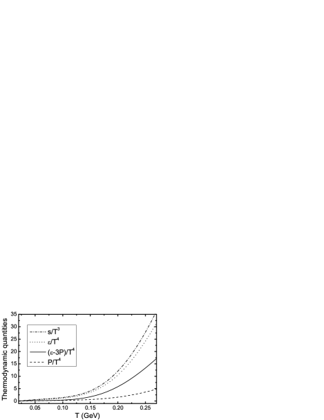
Figure 2: Some scaled thermodynamic quantities (the entropy density $s$, the energy density $\varepsilon$, the pressure $P$) and the trace of the energy-momentum tensor of the ideal gas with the hadron gas mass spectrum including 322 particle species.

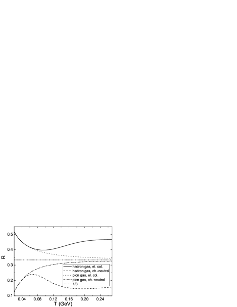
Figure 3: The quantity $R$ (51), appearing in the bulk viscosity source term (58), ate zero chemical potentials. In the case of the charge-neutral (or chargeless) system the $R$ coincides with the squared speed of sound $\upsilon_{s}^{2}=\frac{\partial P}{\partial\varepsilon}$. In the case of only the elastic collisions it is given by the (V.1). It is calculated for the ideal hadron gas in the first and the second cases (solid and dashed lines correspondingly) and the ideal pion gas (doted and dash-dotted lines correspondingly). The value of $1/3$ is shown for convenience (dash-dot-dotted line).

The results for the shear and the bulk viscosities are shown in fig. 4 and fig. 5 correspondingly. They are calculated with the different cross sections (with all corrections and fixes): ECQs, EQCSs, EQCS2s, TCSs, TCS2s. They are described in Sec. III. The bulk viscosity with the TCS2s is not shown because it’s smaller only on $5\%$ or less than the one with the TCSs. Up to 5 (3) test-functions are used in the calculations of the bulk (shear) viscosity. The maximal errors are $11\%$ and are less than $4.2\%$ outside the range $40~{}MeV\leq T\leq 90~{}MeV$. The best convergence is for the case of the ECSs (the errors are less than $2\%$). For quantitative results the recommended cross sections are the EQCS2s, as is commented in Sec. III. For qualitative analysis the TCSs and the TCS2s are more suitable. Also it’s shown that the approximation of one constant cross section for all hadrons is a good one. For the shear viscosity with the EQCSs or the EQCS2s it’s somewhat worse. This can be explained in the following way. There are descending and growing cross sections, and these opposite dependencies compensate approximately each other, so that at some temperatures the cross sections manifest themselves approximately as a constant one. Some EQCSs and EQCS2s have quite steeply descending tails, which explains relatively fast rises in the shear viscosities, because of which one constant cross section doesn’t provides worse approximation. An explanation why the bulk viscosity is approximated well in the same case with one constant cross sections at some temperatures would be somewhat more complicated.

Also the calculations without resonances (the particles with the width larger or equal to $0.2~{}MeV$) are done with the EQCSs to find out the magnitude of their contributions. After the exclusion 26 particle species remain. The bulk viscosity decreases not more than in 2.8 times, and the shear viscosity decreases not more than in 1.6 times (using the TCSs these factors are somewhat smaller).

Note that at $T\approx 160~{}MeV$ the viscosities calculated with the TCS2s are approximately 2 times smaller than the viscosities calculated with the EQCS2s respectively. This reflects the fact that the contribution to the total number of collisions from the inelastic processes is approximately the same as from the elastic plus the quasielastic processes at the freeze-out temperature.

The maximum of the bulk viscosity is, of course, sensitive to the energy dependence of the cross sections, as can be seen from fig. 5. E. g. if the BB and some MB EQCSs were not fixed, as is described in Sec. III, the maximum would be present at $T\approx 190~{}MeV$. After the fixes the BB and some MB EQCSs and EQCS2s have steeply descending tails, and the maximum shifts towards much higher temperatures. Though for the qualitative analysis the TCSs and the TCS2s are more suitable because at $T\gtrsim 160~{}MeV$ the inelastic processes make not small contributions. With these cross sections the bulk viscosity has the maximum at $T\approx 190~{}MeV$. With one constant cross section the maximum is present at $T\approx 200~{}MeV$ with Moroz:2011vn or without charmed and bottomed particles.

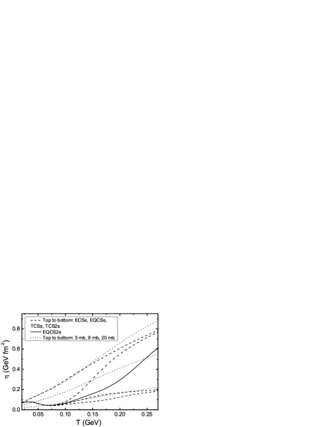
Figure 4: The shear viscosity of the hadron gas, calculated with the ECSs, EQCSs, TCSs, TCS2s (dashed line) and the EQCS2s (solid line). One constant cross section for all hadrons is used in the approximating calculations. Different values are chosen: $5~{}mb$, $8~{}mb$, $20~{}mb$ (dotted line). See text for more details.

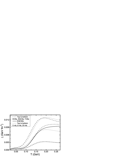
Figure 5: The bulk viscosity of the hadron gas, calculated with the ECSs, EQCSs, TCSs (dashed line) and the EQCS2s (solid line). One constant cross section for all hadrons is used in the approximating calculations. Different values are chosen: $5~{}mb$, $8~{}mb$, $20~{}mb$ (dotted line). See text for more details.

In several papers the viscosities of the hadron gas were studied by the ones of the pion gas. This approximations turn out to be bad while calculating the bulk viscosity. In fig. 6 the ratio of the bulk viscosity of the hadron gas to the one of the pion gas, using different cross sections, is shown. With all the used cross sections the deviations are quite large. Purely pion gas implies the ECSs. The bulk viscosity of the hadron gas with the EQCS2s is divided on the one of the pion gas with the EQCS. This ratio reaches 122 at $T=270~{}MeV$. Considering a closer to the pion gas approximation, excluding the resonances in the hadron gas, this ratio becomes $2.3-2.6$ times smaller at $T=120-140~{}MeV$. The same factor is equal to $2.0-2.1$ for the used TCS2s and the TCSs for the hadron gas and the pion gas correspondingly. Though the resonances should not be excluded. At the same time the corresponding ratios of the particle number densities and the energy densities at $T=140~{}MeV$ are approximately equal to 2 and 3 respectively. Note that the ratios of the viscosities are less sensitive to the corrections discussed in Sec. IV than the viscosities themselves. The ratio of the shear viscosity of the hadron gas to the one of the pion gas is not larger than 1.6, as can be seen in fig. 7. It can even be somewhat smaller than 1 if the TCS2s and the TCS2 are used. This seems to be because the shear viscosity is not much sensitive to the mass spectrum as the bulk viscosity, and the contributions from the hadrons other than pions at high temperatures (where pion numbers don’t dominate) come with somewhat larger (on average) cross sections.

Some simplified explanations of the enlarged bulk viscosity in the hadron gas (to some extent) and the position of its maximum can be made. The bulk viscosity is sensitive to particle’s masses $m\sim T$, and the hadron gas mass spectrum provides such masses at different temperatures. For a fixed $m/T$ and approximately constant cross section the bulk viscosity grows with the temperature, as can be seen from the formula (107), using it as an estimate. Particles with very large masses have relatively small number densities because of the exponential suppression $e^{-m/T}$ so that the maximum is set by particles with not the largest masses at $T\approx 190~{}MeV$, and a relatively slow further descending follows at higher temperatures.

Figure 6: The ratio of the bulk viscosity of the hadron gas to the one of the pion gas. The different cross sections are used: TCS2s/TCSs (dashed line), EQCS2s/EQCSs (solid line), ECSs/ECSs (dotted line). See text for more details.

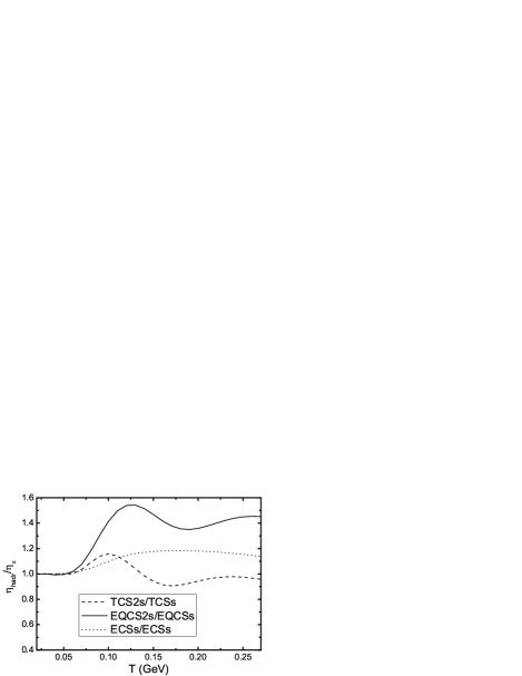
Figure 7: The ratio of the shear viscosity of the hadron gas to the one of the pion gas. The different cross sections are used: TCS2s/TCSs (dashed line), EQCS2s/EQCSs (solid line), ECSs/ECSs (dotted line). See text for more details.

The ratio of the shear viscosity to the entropy density $\eta/s$ and the ratio of the bulk viscosity to the entropy density $\xi/s$ in the hadron gas are shown in fig. 8. The EQCS2s are used. As long as the maximum of the bulk viscosity is not sharp, the ratio $\xi/s$ doesn’t have a maximum and is a descending function of the temperature. The entropy density is calculated by the formula (176) using the ideal gas formulas in the (22) and the (V.1). The ratio of the bulk viscosity to the shear viscosity with the EQCS2s is shown in fig. 9.

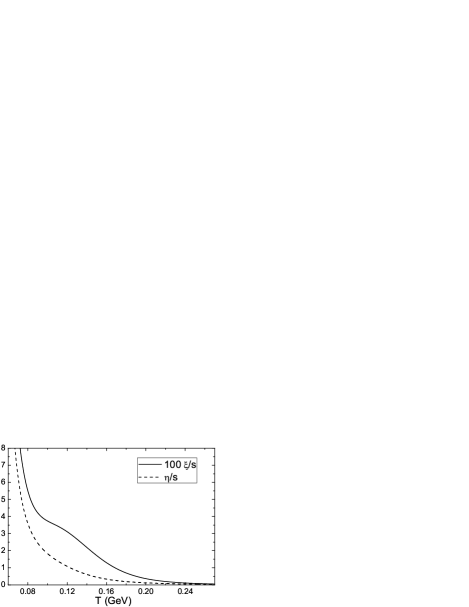
Figure 8: The ratio of the shear viscosity to the entropy density and the ratio of the bulk viscosity times 100 to the entropy density in the hadron gas. The EQCS2s are used.

Figure 9: The ratio of the bulk viscosity times 100 to the shear viscosity in the hadron gas. The EQCS2s are used.

The dependencies from the temperature of the $\eta/s$ and the $\xi/s$ calculated along the chemical freeze-out line are found too and are depicted in fig. 10. The EQCS2s are used. As was discussed in Sec. IV, the calculations with large chemical potentials may contain large deviations, especially in the bulk viscosity, however, in the hadron gas the contributions from the bosons and the fermions may cancel substantially. The calculations along the chemical freeze-out line could have not small deviations for the bulk viscosity because of the inelastic processes. At the considered collision energies the strange particle numbers are not described well by the equilibrium statistical calculations. It’s expected that this is because they don’t reach the chemical equilibrium before the chemical freeze-out takes place. After the introduction of the strange saturation factors $\gamma_{s}$ Becattini:2005xt the experimental data gets described better. As long as the considered chemical perturbations are not quite accurate and are not small they are used in a phenomenological way, being inserted into all particle number densities. Because of all this the calculations along the chemical freeze-out line are less reliable than the ones at zero chemical potentials.

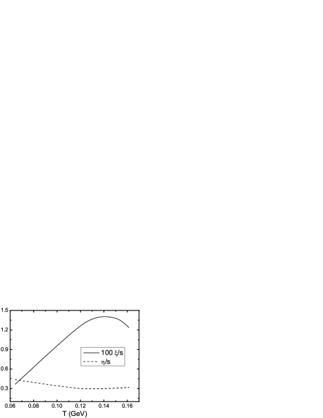
Figure 10: The ratio of the bulk viscosity times 100 to the entropy density and the ratio of the shear viscosity to the entropy density as functions of the freeze-out values of the temperature $T$. All other freeze-out line variables’ values can be found in the Gorenstein:2007mw . The EQCS2s are used.

All variables’ values of the chemical freeze-out line, including the strangeness saturation factor $\gamma_{s}$, are conveniently presented in the Gorenstein:2007mw . The convergence of the calculations (with all the cross section types) is good with the errors less than $4\%$ for both the viscosities. Also it was checked how the results change if the chemical equilibrium is assumed. The entropy density increases up to $36\%$. The shear viscosity increases no more than on $13\%$. The bulk viscosity decreases no more than on $5.1\%$ (though with the ECSs the decrease would be on $44\%$).

VII Analytical results

VII.1 The single-component gas

In the single-component gas, using one test-function, the matrix equations can be easily solved, and the shear (92) and the bulk (103) viscosities become (indexes ”1” of the particle species are omitted)

$$\eta=\frac{1}{10}\frac{T}{\sigma(T)}\frac{(\gamma^{0})^{2}}{C^{00}},$$ (104)

$$\xi=\frac{T}{\sigma(T)}\frac{(\alpha^{2})^{2}}{A^{22}}.$$ (105)

In this approximation the explicit closed-form (expressed through special and elementary functions) relativistic formulas for the bulk and the shear viscosities were obtained in the anderson . There the parameter ${a=2r}$. In groot (Chap. XI, Sec. 1) they are written through the parameter ${\sigma=2r^{2}}$. The results are

$$\eta=\frac{15}{64\pi}\frac{T}{r^{2}}\frac{z^{2}K_{2}^{2}(z)\hat{h}^{2}}{(5z^{2}+2)K_{2}(2z)+(3z^{3}+49z)K_{3}(2z)},$$ (106)

$$\xi=\frac{1}{64\pi}\frac{T}{r^{2}}\frac{z^{2}K_{2}^{2}(z)[(5-3\gamma)\hat{h}-3\gamma]^{2}}{2K_{2}(2z)+zK_{3}(2z)},$$ (107)

where ${\gamma=\frac{1}{c_{\upsilon}}+1=\frac{z^{2}+5\hat{h}-\hat{h}^{2}}{z^{2}+5\hat{h}-\hat{h}^{2}-1}}$. Though the correct result for the shear viscosity is

$$\eta=\frac{15}{64\pi}\frac{T}{r^{2}}\frac{z^{2}K_{2}^{2}(z)\hat{h}^{2}}{(15z^{2}+2)K_{2}(2z)+(3z^{3}+49z)K_{3}(2z)}.$$ (108)

This result is in agreement with the result in prakash ; leeuwen . To get the (108) and the (107) the collision brackets in the $C^{00}$ (96) and the $A^{22}$ (95) can be taken from Appendix C with ${z_{k}=z_{l}=z}$ and the $\gamma^{0}$ and $\alpha^{2}$ can be taken from Appendix A. In the nonrelativistic limit, ${z\gg 1}$, one gets

$$\eta=\frac{5}{64\sqrt{\pi}}\frac{T}{r^{2}}\sqrt{z}\left(1+\frac{25}{16}z^{-1}+...\right),$$ (109)

$$\xi=\frac{25}{256\sqrt{\pi}}\frac{T}{r^{2}}z^{-3/2}\left(1-\frac{183}{16}z^{-1}+...\right).$$ (110)

In the ultrarelativistic limit, ${z\ll 1}$, one gets

$$\eta=\frac{3}{10\pi}\frac{T}{r^{2}}\left(1+\frac{1}{20}z^{2}+...\right),$$ (111)

$$\xi=\frac{1}{288\pi}\frac{T}{r^{2}}z^{4}\left(1+\left(\frac{49}{12}-6\ln 2+6\gamma_{E}\right)z^{2}+6z^{2}\ln z+...\right),$$ (112)

where $\gamma_{E}$ is the Euler’s constant, ${\gamma_{E}\approx 0.577}$.

The perturbation of the distribution function $\varphi$ (68) can be found too:

$$\varphi=\frac{1}{n\sigma(T)}\left(-(A^{0}+A^{1}\tau+A^{2}\tau^{2})\nabla_{\mu}U^{\mu}+C^{0}\overset{\circ}{\overline{\pi^{\mu}\pi^{\nu}}}\overset{\circ}{\overline{\nabla_{\mu}U_{\nu}}}\right),$$ (113)

where the $C^{0}$ is equal to

$$C^{0}=\frac{15}{64\pi}\frac{\sigma(T)}{r^{2}}\frac{z^{2}K_{2}^{2}(z)\hat{h}}{(15z^{2}+2)K_{2}(2z)+(3z^{3}+49z)K_{3}(2z)},$$ (114)

and the $A^{2}$ is equal to

$$A^{2}=\frac{1}{64\pi}\frac{\sigma(T)}{r^{2}}\frac{z^{2}K_{2}^{2}(z)[(5-3\gamma)\hat{h}-3\gamma]}{2K_{2}(2z)+zK_{3}(2z)}.$$ (115)

The $A^{0}$ and the $A^{1}$ are used to satisfy the matching conditions (76) and are equal to

$$A^{0}=A^{2}\frac{a^{2}a^{4}-(a^{3})^{2}}{\Delta_{A}},\quad A^{1}=A^{2}\frac{a^{2}a^{3}-a^{1}a^{4}}{\Delta_{A}},\quad\Delta_{A}\equiv a^{1}a^{3}-(a^{2})^{2},$$ (116)

where the $a^{s}$ can be found in Appendix A. In the nonrelativistic limit ${z\gg 1}$ one has

$$\varphi=\frac{5\pi e^{z-\hat{\mu}}}{32\sqrt{2}T^{3}z^{2}r^{2}}\left(-(\tau^{2}+2z\tau-z^{2})\nabla_{\mu}U^{\mu}+2\overset{\circ}{\overline{\pi^{\mu}\pi^{\nu}}}\overset{\circ}{\overline{\nabla_{\mu}U_{\nu}}}\right).$$ (117)

In the ultrarelativistic limit $z\ll 1$ one has

$$\varphi=\frac{\pi e^{-\hat{\mu}}}{480T^{3}r^{2}}\left(-5z^{2}(\tau^{2}+8\tau-12)\nabla_{\mu}U^{\mu}+36\overset{\circ}{\overline{\pi^{\mu}\pi^{\nu}}}\overset{\circ}{\overline{\nabla_{\mu}U_{\nu}}}\right).$$ (118)

Note that although the shear viscosity diverges for ${T\rightarrow\infty}$ the perturbative expansion over the gradients does not break down because the $\varphi$ does not diverge (it tends to zero, conversely).

The phenomenological formula, coming from the momentum transfer considerations in the kinetic-molecular theory, for the shear viscosity is ${\eta_{ph}\propto ln\langle\left|\vec{p}\right|\rangle}$ (with the coefficient of proportionality of order 1), where $\langle\left|\vec{p}\right|\rangle$ is the average relativistic momentum (11), $l$ is the mean free path. It gives the correct leading $m$ and $T$ parameter dependence of the (108) with a quite precise coefficient. The mean free path can be estimated as ${l\approx 1/(\sigma_{tot}n)}$ (see Appendix D). Choosing the coefficient of proportionality to match the nonrelativistic limit one gets Gorenstein:2007mw

$$\eta_{ph}=\frac{5}{64\sqrt{\pi}}\frac{\sqrt{mT}}{r^{2}}\frac{K_{5/2}(m/T)}{K_{2}(m/T)}.$$ (119)

If the bulk viscosity is expressed as ${\xi_{ph}\propto ln\langle\left|\vec{p}\right|\rangle}$ the coefficient of proportionality is not of order 1. In the nonrelativistic limit it is $25/(512\sqrt{2}z^{2})$ and in the ultrarelativistic limit it is $z^{4}/(864\pi)$. To reproduce these asymptotical dependencies the bulk viscosity should be proportional to the second power of the averaged product of the source term $\hat{Q}$ and the $\tau$ that is to the $(\alpha^{2})^{2}$.

If a system has no charges, then terms proportional to the $\tau_{k}$ in the (58) are absent, and the $R$ quantity gets another form. This results in quite different values of the $\alpha_{k}^{r}$. In particular, for the single-component gas in the case ${z\gg 1}$ one gets

$$\frac{(\alpha^{2})^{2}|_{q_{11}=0}}{(\alpha^{2})^{2}|_{q_{11}=1}}=\frac{4z^{4}}{25}+...,$$ (120)

and in the case ${z\ll 1}$ one gets

$$\frac{(\alpha^{2})^{2}|_{q_{11}=0}}{(\alpha^{2})^{2}|_{q_{11}=1}}=4+....$$ (121)

In both cases these estimates suppose enhancement of the bulk viscosity (105) if the number-changing processes are not negligible.

Although constant cross sections are the most simple and the most universal ones in approximate calculations, let’s write down also formulas for some other simple energy dependencies of cross sections. Using the collision bracket from Appendix C, one gets for the cross section $\sigma s/(2m)^{2}=\sigma\upsilon^{2}/(2z)^{2}$ ($\sigma$ is just a positive dimensional constant here)

$$\eta_{1}=\frac{15T}{32\pi\sigma}\frac{\hat{h}^{2}z^{3}K_{2}^{2}(z)}{9z(3z^{2}+34)K_{2}(2z)+(3z^{4}+157z^{2}+920)K_{3}(2z)},$$ (122)

$$\xi_{1}=\frac{T}{32\pi\sigma}\frac{z^{3}[(5-3\gamma)\hat{h}-3\gamma]^{2}K_{2}^{2}(z)}{(z^{2}+20)K_{3}(2z)+6zK_{2}(2z)},$$ (123)

and for the cross section $\sigma(2m)^{2}/s=\sigma(2z)^{2}/\upsilon^{2}$:

$$\eta_{2}=\frac{15T}{32\pi\sigma}\frac{\hat{h}^{2}z^{2}K_{2}^{2}(z)}{(3z^{2}-2)K_{2}(2z)+z(3z^{2}+1)K_{3}(2z)},$$ (124)

$$\xi_{2}=\frac{T}{32\pi\sigma}\frac{z^{2}[(5-3\gamma)\hat{h}-3\gamma]^{2}K_{2}^{2}(z)}{(zK_{3}(2z)-2K_{2}(2z))}.$$ (125)

Using the low-energy current algebra isospin averaged $\pi\pi$ differential cross section prakash ; Weinberg:1966kf

$$\sigma_{CA}=\frac{1}{3}\frac{s}{64\pi^{2}f_{\pi}^{4}}\left[3-8\frac{m_{\pi}^{2}}{s}+7\frac{m_{\pi}^{4}}{s^{2}}+\left(1-8\frac{m_{\pi}^{2}}{s}+16\frac{m_{\pi}^{4}}{s^{2}}\right)\cos^{2}\Theta\right],$$ (126)

($f_{\pi}=93~{}MeV$ is the pion decay constant) and treating all pions as identical particles at zero chemical potentials, one gets the formulas

$$\eta_{CA}=\frac{360\pi f_{\pi}^{4}}{T}\frac{\hat{h}^{2}zK_{2}^{2}(z)}{9z(93z^{2}+1730)K_{2}(2z)+(69z^{4}+6167z^{2}+47104)K_{3}(2z)},$$ (127)

$$\xi_{CA}=\frac{24\pi f_{\pi}^{4}}{T}\frac{z[(5-3\gamma)\hat{h}-3\gamma]^{2}K_{2}^{2}(z)}{(23z^{2}+1024)K_{3}(2z)+210zK_{2}(2z)},$$ (128)

which are exactly 2 times larger than the 1-st order calculations in the prakash . Taking the scattering angle averaged cross section instead of the (126), one would get approximately the same result for the viscosities (errors are not more than $4\%$). In the low temperature limit, $z\gg 1$, one gets the following expansions for the shear viscosities (122), (124), (127):

$$\eta_{1}=\frac{5}{32\sqrt{\pi}}\frac{T}{\sigma}\sqrt{z}\left(1-\frac{39}{16}z^{-1}+...\right),$$ (129)

$$\eta_{2}=\frac{5}{32\sqrt{\pi}}\frac{T}{\sigma}\sqrt{z}\left(1+\frac{89}{16}z^{-1}+...\right),$$ (130)

$$\eta_{CA}=\frac{120\pi^{3/2}}{23}\frac{f_{\pi}^{4}}{T}z^{-3/2}\left(1-\frac{2049}{368}z^{-1}+...\right),$$ (131)

and in the high temperature limit, $z\ll 1$, respectively:

$$\eta_{1}=\frac{3}{92\pi}\frac{T}{\sigma}z^{2}\left(1-\frac{2}{23}z^{2}+...\right),$$ (132)

$$\eta_{2}=\frac{6}{\pi}\frac{T}{\sigma}z^{-2}\left(1+\frac{1}{20}(9-4\gamma_{E})z^{2}-\frac{1}{5}z^{2}\ln z+...\right),$$ (133)

$$\eta_{CA}=\frac{45\pi}{92}\frac{f_{\pi}^{4}}{T}\left(1-\frac{17}{368}z^{2}+...\right).$$ (134)

In the low temperature limit, $z\gg 1$, one gets the following expansions for the bulk viscosities (123), (125), (128):

$$\xi_{1}=\frac{25}{128\sqrt{\pi}}\frac{T}{\sigma}z^{-3/2}\left(1-\frac{247}{16}z^{-1}+...\right),$$ (135)

$$\xi_{2}=\frac{25}{128\sqrt{\pi}}\frac{T}{\sigma}z^{-3/2}\left(1-\frac{119}{16}z^{-1}+...\right),$$ (136)

$$\xi_{CA}=\frac{150\pi^{3/2}}{23}\frac{f_{\pi}^{4}}{T}z^{-7/2}\left(1-\frac{6833}{368}z^{-1}+...\right),$$ (137)

and in the high temperature limit, $z\ll 1$, respectively:

$$\xi_{1}=\frac{1}{1440\pi}\frac{T}{\sigma}z^{6}\left(1+\frac{1}{30}(109+180\gamma_{E}-180\ln 2)z^{2}+6z^{2}\ln z...\right),$$ (138)

$$\xi_{2}=\frac{1}{36\pi}\frac{T}{\sigma}z^{2}\left(1+\frac{1}{3}(13+12\gamma_{E}-18\ln 2)z^{2}+4z^{2}\ln z+...\right),$$ (139)

$$\xi_{CA}=\frac{\pi}{96}\frac{f_{\pi}^{4}}{T}z^{4}\left(1+\frac{1}{24}(89+144\gamma_{E}-144\ln 2)z^{2}+6z^{2}\ln z+...\right).$$ (140)

Let’s also write down the viscosities with the cross section $\sigma[1+c_{1}\upsilon^{2}/(2z)^{2}+c_{2}(2z)^{2}/\upsilon^{2}]$, unifying the previously considered ones:

$$\eta_{3} = \frac{15}{32\pi\sigma}T\hat{h}^{2}z^{3}K^{2}_{2}(z)/[z(2+306c_{1}-2c_{2}+3(5+9c_{1}+c_{2})z^{2})K_{2}(2z)$$ (141)

$$+ (920c_{1}+(49+157c_{1}+c_{2})z^{2}+3(1+c_{1}+c_{2})z^{4})K_{3}(2z)],$$

$$\xi_{3}=\frac{T}{32\pi\sigma}\frac{z^{3}[(5-3\gamma)\hat{h}-3\gamma]^{2}K^{2}_{2}(z)}{2(1+3c_{1}-c_{2})zK_{2}(2z)+(20c_{1}+(1+c_{1}+c_{2})z^{2})K_{3}(2z)},$$ (142)

where $c_{1}$ and $c_{2}$ are some dimensionless coefficients such that $c_{1}+c_{2}+1\geq 0$ and $c_{1}\geq 0$ to make the cross section non-negative. The last formulas may have badly convergent expansions over the $z$ and the $z^{-1}$ for some values of the $c_{1}$ and the $c_{2}$ so that they ain’t expanded.

VII.2 The binary mixture

The mixture of two species with masses $m_{1}$, $m_{2}$ and the different classical elastic differential constant cross sections $\sigma^{cl}_{11}$, ${\sigma^{cl}_{12}=\sigma^{cl}_{21}}$, $\sigma^{cl}_{22}$ is considered in this section. Using the (92) with ${n_{2}=0}$ and solving the matrix equation (94) one gets for the shear viscosity

$$\eta=\frac{T}{10\sigma(T)}\frac{1}{\Delta_{\eta}}[(x_{1^{\prime}}\gamma_{1}^{0})^{2}C_{2^{\prime}2^{\prime}}^{00}-2x_{1^{\prime}}x_{2^{\prime}}\gamma_{1}^{0}\gamma_{2}^{0}C_{1^{\prime}2^{\prime}}^{00}+(x_{2^{\prime}}\gamma_{2}^{0})^{2}C_{1^{\prime}1^{\prime}}^{00}],$$ (143)

where ${\Delta_{\eta}=C_{1^{\prime}1^{\prime}}^{00}C_{2^{\prime}2^{\prime}}^{00}-(C_{1^{\prime}2^{\prime}}^{00})^{2}}$. The collision brackets for the $C_{k^{\prime}l^{\prime}}^{00}$ (96) can be found in Appendix C and the $\gamma_{k}^{0}$ can be found in Appendix A.

In the important limiting case when one mass is large ${z_{2}\gg 1}$ ($g_{2}$ and $\hat{\mu}_{2}$ are finite so that ${x_{2^{\prime}}\ll 1}$) and another mass is finite one can perform asymptotic expansion of the special functions. Then one has ${x_{1^{\prime}}\propto O(1)}$, ${\gamma_{1}^{0}\propto O(1)}$, ${x_{2^{\prime}}\propto O(e^{-z_{2}}z_{2}^{3/2})}$, ${\gamma_{2}^{0}\propto O(z_{2})}$. The collisions of light and heavy particles dominate over the collisions of heavy and heavy particles in the $C_{2^{\prime}2^{\prime}}^{00}$, and one has ${[\overset{\circ}{\overline{\pi^{\mu}\pi^{\nu}}},\overset{\circ}{\overline{\pi_{\mu}\pi_{\nu}}}]_{21}\propto O(z_{2})}$, ${C_{2^{\prime}2^{\prime}}^{00}\propto O(e^{-z_{2}}z_{2}^{5/2})}$. In the $C_{1^{\prime}1^{\prime}}^{00}$ the collisions of light and light particles dominate, and one gets ${C_{1^{\prime}1^{\prime}}^{00}\propto O(1)}$. And ${[\overset{\circ}{\overline{\pi^{\mu}\pi^{\nu}}},\overset{\circ}{\overline{\pi_{1\mu}\pi_{1\nu}}}]_{12}\propto O(1)}$, ${C_{1^{\prime}2^{\prime}}^{00}\propto O(e^{-z_{2}}z_{2}^{3/2})}$. In the shear viscosity the first nonvanishing contribution is the single-component shear viscosity (108), where one should take ${r^{2}=\sigma^{cl}_{11}}$ and ${z=z_{1}}$. The next correction is

$$\Delta\eta=z_{2}^{5/2}e^{-z_{2}}\frac{3Tg_{2}e^{z_{1}-\hat{\mu}_{1}+\hat{\mu}_{2}}}{64\sqrt{2\pi}(3+3z_{1}+z_{1}^{2})g_{1}\sigma^{cl}_{12}}.$$ (144)

The approximate formula Gorenstein:2007mw

$$\eta=\sum_{k}\eta_{k}x_{k},$$ (145)

where $\eta_{k}$ is given by the (108) or the (119) with mass $m_{k}$ and cross section $\sigma^{cl}_{kk}$, would give somewhat different heavy mass power dependence $O(e^{-z_{2}}z_{2}^{2})$.

Using the (103) with ${n_{1}=1}$ and solving the matrix equation (102) one gets for the bulk viscosity

$$\xi=\frac{T}{\sigma(T)}\frac{(x_{2^{\prime}}\alpha_{2}^{1})^{2}}{A_{2^{\prime}2^{\prime}}^{11}}=\frac{T}{\sigma(T)}\frac{x_{1^{\prime}}x_{2^{\prime}}\alpha_{1}^{1}\alpha_{2}^{1}}{A_{1^{\prime}2^{\prime}}^{11}}.$$ (146)

Using the definition of the $A_{2^{\prime}2^{\prime}}^{11}$ (95) and the fact ${[\tau,\tau_{1}]_{kl}+[\tau,\tau]_{kl}=0}$ (210) one gets ${A_{2^{\prime}2^{\prime}}^{11}=x_{1^{\prime}}x_{2^{\prime}}[\tau,\tau]_{12}}$. Using the (98) one gets ${[\tau,\tau]_{12}>0}$. Then using ${x_{1^{\prime}}\alpha_{1}^{1}+x_{2^{\prime}}\alpha_{2}^{1}=0}$, coming from the (65), the bulk viscosity can be rewritten as

$$\xi=\frac{T}{\sigma(T)}\frac{x_{2^{\prime}}(\alpha_{2}^{1})^{2}}{x_{1^{\prime}}[\tau,\tau]_{12}}=\frac{T}{\sigma(T)}\frac{x_{1^{\prime}}(\alpha_{1}^{1})^{2}}{x_{2^{\prime}}[\tau,\tau]_{12}}>0.$$ (147)

The collision bracket $[\tau,\tau]_{12}$ can be found in Appendix C, and the $\alpha_{k}^{1}$ can be found in Appendix A.

In the limiting case ${z_{2}\gg 1}$ one has ${x_{1^{\prime}}\propto O(1)}$, ${x_{2^{\prime}}\propto O(e^{-z_{2}}z_{2}^{3/2})}$, ${\alpha_{1}^{1}\propto O(e^{-z_{2}}z_{2}^{3/2})}$, ${\alpha_{2}^{1}\propto O(1)}$, ${A_{22}^{11}\propto A_{12}^{11}\propto O(e^{-z_{2}}z_{2}^{1/2})}$, ${[\tau,\tau]_{12}\propto O(z_{2}^{-1})}$. Then for the bulk viscosity one gets

$$\xi=e^{-z_{2}}z_{2}^{5/2}\frac{g_{2}Te^{-\hat{\mu}_{1}+\hat{\mu}_{2}+z_{1}}[2z_{1}^{2}-5-2\hat{h}_{1}^{2}+10\hat{h}_{1}]^{2}}{128\sqrt{2\pi}g_{1}\sigma^{cl}_{12}(z_{1}^{2}+3z_{1}+3)[z_{1}^{2}-1-\hat{h}_{1}^{2}+5\hat{h}_{1}]^{2}}+....$$ (148)

VIII Concluding remarks

The shear and the bulk viscosities of the hadron gas and the pion gas were calculated using the UrQMD cross sections.

The physics of the bulk viscosity is very interesting. In particular, in mixtures it can strongly depend on the mass spectrum. For instance, at the temperature ${T=120~{}MeV}$ (${140~{}MeV}$) and zero chemical potentials the bulk viscosity of the hadron gas is larger in 8.6-15.6 (14.6-40) times than the bulk viscosity of the pion gas. The used UrQMD cross sections have allowed to perform this comparison more accurately.

Also the bulk viscosity can strongly depend on the quantum statistics corrections, the equation of state and the inelastic processes, which can be explained by nontrivial form of its source term(s). It’s a future task to find the universal and optimal criterion for switching on/off the inelastic processes. Numerical calculations of the bulk viscosity along and around the chemical freeze-out line which don’t involve the approximations of conserved or not conserved particle numbers (like in the Muronga:2003tb , though the procedure of collisions of particles introduce some errors itself, which should be kept in mind) are desirable to get more accurate values of the bulk viscosity at these points. This is also needed for a better understanding of the chemical freeze-out itself and connected with it problems and to get a better description of the deviations from the chemical equilibrium.

The transport coefficients are connected with fluctuations through the fluctuation-dissipation theorem. Because of strong dependence of the bulk viscosity on the equation of state one might expect to find its maximum at or near a phase transition point. According to lattice calculations at zero chemical potentials Aoki:2006we , the QCD phase transition is an analytical crossover. Calculations of the Polyakov loop Hidaka:2008dr , the ’t Hooft loop Dumitru:2010mj and some other calculations Ratti:2011au suggest that hadronic degrees of freedom survive partially at some temperatures above the critical one. In the qualitative calculations for the hadron gas with the UrQMD total cross sections the maximum of the bulk viscosity has been found at $T\approx 190~{}MeV$. This value fits in the transition temperature range $T_{c}=185-195~{}MeV$ found from lattice calculations by the hotQCD collaboration, but calculations of the Wuppertal-Budapest collaboration with physical quark masses give the region $T_{c}=150-170~{}MeV$ Borsanyi:2010bp . According to the Wuppertal-Budapest collaboration calculations of thermodynamic functions with physical quark masses Borsanyi:2010cj , the scaled trace of the energy-momentum tensor has its peak at $T\approx 190~{}MeV$. In some other lattice calculations with somewhat different quark masses Cheng:2009zi ; Petreczky:2009ey this peak is somewhat sharper and still is present at $T\approx 190~{}MeV$. According to the lattice calculations in the Borsanyi:2010cj , the squared speed of sound in the charge-neutral hadron gas (implying equal to zero and not developing chemical potentials) has it’s minimum at $T\approx 150~{}MeV$, unlike the ideal gas calculations ($T\approx 190~{}MeV$) or the ones in the toneev ($T\approx 180~{}MeV$). So that one could expect to find the maximum of the bulk viscosity somewhere in the temperature range $T=150-190~{}MeV$, presumably closer to the lowest bound. This range covers the critical temperature values found from the lattice calculations.

The shear viscosity is less dependent on the mass spectrum, the quantum statistics corrections, the equation of state and the inelastic processes. This may be explained by its more trivial source term(s).

Appendix A The values of the $\alpha^{r}_{k}$, $\gamma_{k}^{r}$ and $a_{k}^{r}$

Their definitions are

$$\alpha_{k}^{r}\equiv(\hat{Q}_{k},\tau_{k}^{r}),\quad\gamma_{k}^{r}\equiv(\tau_{k}^{r}\overset{\circ}{\overline{\pi_{k}^{\mu}\pi_{k}^{\nu}}},\overset{\circ}{\overline{\pi_{k\mu}\pi_{k\nu}}}),\quad a^{s}_{k}\equiv(1,\tau_{k}^{s})_{k},$$ (149)

where the round brackets are

$$(F,G)_{k}\equiv\frac{1}{4\pi z_{k}^{2}K_{2}(z_{k})T^{2}}\int_{p_{k}}F(p_{k})G(p_{k})e^{-\tau_{k}}.$$ (150)

Then one can rewrite the $a_{k}^{s}$ as

$$a_{k}^{s}=\frac{1}{z_{k}^{2}K_{2}(z_{k})}\int_{z_{k}}^{\infty}d\tau(\tau^{2}-z_{k}^{2})^{1/2}\tau^{s}e^{-\tau}.$$ (151)

There is a recurrence relation for the $a^{s}_{k}$:

$$a^{s}_{k}=(s+1)a^{s-1}_{k}+z_{k}^{2}a^{s-2}_{k}-(s-2)z_{k}^{2}a^{s-3}_{k}.$$ (152)

It can be derived from the (151) written in the form

$$a_{k}^{s}=\frac{1}{z_{k}^{2}K_{2}(z_{k})}\int_{z_{k}}^{\infty}d\tau(\tau^{2}-z_{k}^{2})^{3/2}\tau^{s-2}e^{-\tau}+z_{k}^{2}a_{k}^{s-2}.$$ (153)

Then after integration by parts the recurrence relation follow. Some values of the $a_{k}^{s}$ are

$$a^{0}_{k}=\frac{1}{z_{k}^{2}}(\hat{h}_{k}-4),$$ (154)

$$a^{1}_{k}=1,$$ (155)

$$a^{2}_{k}=\hat{h}_{k}-1,$$ (156)

$$a^{3}_{k}=3\hat{h}_{k}+z_{k}^{2},$$ (157)

$$a^{4}_{k}=(15+z_{k}^{2})\hat{h}_{k}+2z_{k}^{2},$$ (158)

$$a^{5}_{k}=6(15+z_{k}^{2})\hat{h}_{k}+z_{k}^{2}(15+z_{k}^{2}),$$ (159)

$$a^{6}_{k}=(630+45z_{k}^{2}+z_{k}^{4})\hat{h}_{k}+5z_{k}^{2}(21+z_{k}^{2}).$$ (160)

The $\alpha_{k}^{r}$ can be expressed through the $a^{r}_{k}$ after the integration of the (58) (or the (59) if only the elastic collisions are considered) over the momentum, using the definition (149). For systems with only the elastic collisions some values of the $\alpha_{k}^{r}$ are written below, in agreement with groot (Chap. VI, Sec. 3):

$$\alpha_{k}^{0}=0,$$ (161)

$$\alpha_{k}^{1}=\frac{2(c_{\upsilon}-9)\hat{h}_{k}+3\hat{h}_{k}^{2}-3z_{k}^{2}}{c_{\upsilon}}=\frac{\gamma_{k}-\gamma}{\gamma_{k}-1},$$ (162)

$$\alpha_{k}^{2}=2\hat{h}_{k}-3\frac{c_{\upsilon,k}}{c_{\upsilon}}-3\frac{\hat{h}_{k}+1}{c_{\upsilon}}=(5-3\gamma)\hat{h}_{k}-3\gamma_{k}\frac{\gamma-1}{\gamma_{k}-1},$$ (163)

where the assignments $\gamma$ and $\gamma_{k}$ from groot are used. They can be expressed through the $c_{\upsilon}$ and the $c_{\upsilon,k}$, defined in the (V.1), as

$$\gamma\equiv\frac{1}{c_{\upsilon}}+1,\quad\gamma_{k}\equiv\frac{1}{c_{\upsilon,k}}+1.$$ (164)

The $\gamma_{k}^{r}$ can be rewritten as

$$\gamma_{k}^{r}=\frac{2}{3}\frac{1}{z_{k}^{2}K_{2}(z_{k})}\int_{z_{k}}^{\infty}d\tau(\tau^{2}-z_{k}^{2})^{5/2}\tau^{r}e^{-\tau}.$$ (165)

Then it can be rewritten through the $a_{k}^{r}$:

$$\gamma_{k}^{r}=\frac{2}{3}(a^{r+4}-2z_{k}^{2}a^{r+2}+z_{k}^{4}a^{r}).$$ (166)

Some values of the $\gamma_{k}^{r}$ are

$$\gamma_{k}^{0}=10\hat{h}_{k},$$ (167)

$$\gamma_{k}^{1}=10(6\hat{h}_{k}+z_{k}^{2}),$$ (168)

$$\gamma_{k}^{2}=10(7z_{k}^{2}+\hat{h}_{k}(42+z_{k}^{2})).$$ (169)

Appendix B The entropy density formula

The Gibbs’s potential is defined as

$$\Phi(P,T)\equiv E(S,V)-ST+PV.$$ (170)

The differential of the energy is defined as

$$dE=TdS-PdV+\sum_{k}\mu_{k}dN_{k}=TdS-PdV+\sum_{a}\mu_{a}dN_{a},$$ (171)

where it is rewritten through the independent chemical potentials and the particle net charges $N_{a}$. Then the differential of the $\Phi$ reads:

$$d\Phi=-SdT+VdP+\sum_{a}\mu_{a}dN_{a}.$$ (172)

Because the $\Phi$ is the function of the intrinsic variables $P$, $T$ and the extrinsic $N_{a}$ the only possible form of it in the thermodynamic limit is

$$\Phi=\sum_{a}N_{a}\phi_{a}(P,T),$$ (173)

where $\phi_{a}$ are unknown functions. Then from the (172) one gets ${\frac{\partial\Phi}{\partial N_{a}}=\mu_{a}}$, which means that ${\phi_{a}=\mu_{a}}$. Then substituting the (173) into the (170) one gets the relation

$$\sum_{a}N_{a}\mu_{a}(P,T)=E(S,V)-ST+PV.$$ (174)

Being written for local infinitesimal volume it transforms into the expression

$$\sum_{a}n_{a}\mu_{a}=\epsilon-sT+P,$$ (175)

from where the entropy density $s$ can be found:

$$s=\frac{\epsilon+P}{T}-\sum_{a}n_{a}\hat{\mu}_{a}.$$ (176)

Appendix C The calculation of the collision brackets

The momentum parametrization and the most transformations of the 12-dimensional integrals used below are taken from groot (Chap. XI and XIII). Let’s start from some assignments. The full momentum is

$$P^{\mu}=p^{\mu}_{k}+p^{\mu}_{1l}={p^{\prime}}^{\mu}_{k}+{p^{\prime}}^{\mu}_{1l}={P^{\prime}}^{\mu}.$$ (177)

The ”relative” momentums before collision $Q^{\mu}$ and after collision ${Q^{\prime}}^{\mu}$ are defined as

$$Q^{\mu}=\Delta_{P}^{\mu\nu}(p_{k\nu}-p_{1l\nu}),\quad{Q^{\prime}}^{\mu}=\Delta_{P}^{\mu\nu}({p^{\prime}}_{k\nu}-{p^{\prime}}_{1l\nu}),$$ (178)

with the assignment

$$\Delta_{P}^{\mu\nu}=g^{\mu\nu}-\frac{P^{\mu}P^{\nu}}{P^{2}},$$ (179)

where $P^{2}\equiv P^{\mu}P_{\mu}$. The covariant cosine of the scattering angle can be expressed through the $Q^{\mu}$ and the ${Q^{\prime}}^{\mu}$ as

$$\cos\Theta=-\frac{Q\cdot Q^{\prime}}{\sqrt{-Q^{2}}\sqrt{-{Q^{\prime}}^{2}}},$$ (180)

where $\cdot$ denotes convolution of 4-vectors. One also has ${Q^{2}={Q^{\prime}}^{2}}$ and

$$Q^{2}=4m_{k}^{2}-(1+\alpha_{kl})^{2}P^{2}=-\left(P^{2}-M_{kl}^{2}\right)\left[1-\frac{M_{kl}^{2}}{P^{2}}\left(1-\frac{4\mu_{kl}}{M_{kl}}\right)\right],$$ (181)

where

$$M_{kl}\equiv m_{k}+m_{l},\quad\mu_{kl}\equiv\frac{m_{k}m_{l}}{m_{k}+m_{l}},\quad\alpha_{kl}\equiv\frac{m_{k}^{2}-m_{l}^{2}}{P^{2}}=\mathrm{sign}(m_{k}-m_{l})\sqrt{1-\frac{4\mu_{kl}}{M_{kl}}}\frac{M_{kl}^{2}}{P^{2}}.$$ (182)

The function $\mathrm{sign}(x)$ is equal to 1, if ${x>0}$ and equal to $-1$, if ${x<0}$. Note that not all $P^{\mu}$ and $Q^{\mu}$ are independent:

$$P^{\mu}Q_{\mu}=0,\quad P^{\mu}{Q^{\prime}}_{\mu}=0.$$ (183)

To come from the variables ${(p_{k}^{\mu},p_{1l}^{\mu})}$ to the variables ${(P^{\mu},Q^{\mu})}$ in the measure of integration first one has to come from the ${(p_{k}^{\mu},p_{1l}^{\mu})}$ to the ${(p_{k}^{\mu}+p_{1l}^{\mu},p_{k}^{\mu}-p_{1l}^{\mu})}$ (the determinant is equal to $16$) and then shift the relative momentum $p_{k}^{\mu}-p_{1l}^{\mu}$ on the $\alpha_{kl}P^{\mu}$. Analogically for the ${({p^{\prime}}_{k}^{\mu},{p^{\prime}}_{1l}^{\mu})}$ and the ${({P^{\prime}}^{\mu},{Q^{\prime}}^{\mu})}$. The inverse relations for the $p_{k}^{\mu},p_{1l}^{\mu},{p^{\prime}}_{k}^{\mu},{p^{\prime}}_{1l}^{\mu}$ through the $P^{\mu},Q^{\mu},{Q^{\prime}}^{\mu}$ are

$$p_{k}^{\mu}=\frac{1}{2}(1+\alpha_{kl})P^{\mu}+\frac{1}{2}{Q}^{\mu},$$ (184)

$$p_{1l}^{\mu}=\frac{1}{2}(1-\alpha_{kl})P^{\mu}-\frac{1}{2}{Q}^{\mu},$$ (185)

$${p^{\prime}}_{k}^{\mu}=\frac{1}{2}(1+\alpha_{kl})P^{\mu}+\frac{1}{2}{Q^{\prime}}^{\mu},$$ (186)

$${p^{\prime}}_{1l}^{\mu}=\frac{1}{2}(1-\alpha_{kl})P^{\mu}-\frac{1}{2}{Q^{\prime}}^{\mu}.$$ (187)

There is a need to calculate the following integrals

$$J_{kl}^{(a,b,d,e,f|q,r)}\equiv\frac{\gamma_{kl}}{T^{6}(4\pi)^{2}z_{k}^{2}z_{l}^{2}K_{2}(z_{k})K_{2}(z_{l})\sigma(T)}\int_{p_{k},p_{1l},{p^{\prime}}_{k},{p^{\prime}}_{1l}}e^{-P\cdot U/T}(1+\alpha_{kl})^{q}$$ (188)

$$\times(1-\alpha_{kl})^{r}\left(\frac{P^{2}}{T^{2}}\right)^{a}\left(\frac{P\cdot U}{T}\right)^{b}\left(\frac{Q\cdot U}{T}\right)^{d}\left(\frac{Q^{\prime}\cdot U}{T}\right)^{e}\left(\frac{-Q\cdot{Q^{\prime}}}{T^{2}}\right)^{f}W_{kl}.$$

Let’s start from the case of constant cross sections. After nontrivial transformations, described in more details in groot , one arrives at

$$J_{kl}^{(a,b,d,e,f|q,r)}=\frac{\pi(d+e+1)!!\sigma^{(d,e,f)}_{1kl}}{z_{k}^{2}z_{l}^{2}K_{2}(z_{k})K_{2}(z_{l})}\sum_{q_{1}=0}^{q}\sum_{r_{1}=0}^{r}\sum_{k_{2}=0}^{\frac{d+e}{2}+f+1}\sum_{k_{3}=0}^{\frac{d+e}{2}+f+1}\sum_{h=0}^{[b/2]}(z_{k}+z_{l})^{2(q_{1}+r_{1}+k_{2}+k_{3})}$$

$$\times\left(\frac{z_{k}-z_{l}}{z_{k}+z_{l}}\right)^{q_{1}+r_{1}+2k_{3}}(-1)^{r_{1}+k_{2}+k_{3}+h}(2h-1)!!\binom{b}{2h}\binom{q}{q_{1}}\binom{r}{r_{1}}\binom{\frac{d+e}{2}+f+1}{k_{2}}$$

$$\times\binom{\frac{d+e}{2}+f+1}{k_{3}}I\left(2(a+f-q_{1}-r_{1}-k_{2}-k_{3})+3,b+\frac{d+e}{2}-h+1,z_{k}+z_{l}\right),$$

where

$$\sigma_{1kl}^{(d,e,f)}=\frac{\sigma^{cl}_{kl}}{\sigma(T)}\sum_{g=0}^{\min(d,e)}\sigma^{(f,g)}K(d,e,g),$$ (190)

where ${\sigma^{cl}_{kl}=\gamma_{kl}\sigma_{kl}}$ is the classical elastic differential constant cross section. The $\sigma^{(f,g)}$ is equal to the real, nonzero and non-diverging value (for any non-negative integer $g$)

$$\sigma^{(f,g)}=\frac{2g+1}{2}\int_{-1}^{1}dxx^{f}P_{g}(x)=(2g+1)\frac{f!}{(f-g)!!(f+g+1)!!},$$ (191)

if the difference ${f-g}$ is even and ${g\leq f}$. Above the $P_{\text{g}}(x)$ is the Legendre polynomial. The $K(d,e,g)$ is equal to the real, the nonzero and non-diverging quantity (for any non-negative integer $g$)

$$K(d,e,g)=\frac{d!e!}{(d-g)!!(d+g+1)!!(e-g)!!(e+g+1)!!},$$ (192)

if ${g\leq\min(d,e)}$ and both the ${d-g}$ and the ${e-g}$ are even (which also implies that ${d+e}$ is even). The ${[...]}$ denotes the integer part. The integral $I$ is

$$I(r,n,x)\equiv x^{r+n+1}\int_{1}^{\infty}duu^{r+n}K_{n}(xu).$$ (193)

Also there is the following frequently used combination of the $J$ integrals

$${J^{\prime}}_{kl}^{(a,b,d,e,f|q,r)}\equiv\sum_{u=0}^{f}(-1)^{u}\binom{f}{u}(2z_{k})^{2(f-u)}J_{kl}^{(a+k,b,d+e,0,0|q+2u,r)}-J_{kl}^{(a,b,d,e,f|q,r)}.$$ (194)

The first term in the difference is obtained by the replacement of the $Q^{\prime}$ on the $Q$ everywhere except for the $W_{kl}$. Using this fact, the $J^{\prime}$ can be rewritten in the form

$${J^{\prime}}_{kl}^{(a,b,d,e,f|q,r)}=\frac{\pi(d+e-1)!!\sigma^{(d,e,f)}_{kl}}{z_{k}^{2}z_{l}^{2}K_{2}(z_{k})K_{2}(z_{l})}\sum_{q_{1}=0}^{q}\sum_{r_{1}=0}^{r}\sum_{k_{2}=0}^{\frac{d+e}{2}+f+1}\sum_{k_{3}=0}^{\frac{d+e}{2}+f+1}\sum_{h=0}^{[b/2]}(z_{k}+z_{l})^{2(q_{1}+r_{1}+k_{2}+k_{3})}$$

$$\times\left(\frac{z_{k}-z_{l}}{z_{k}+z_{l}}\right)^{q_{1}+r_{1}+2k_{3}}(-1)^{r_{1}+k_{2}+k_{3}+h}(2h-1)!!\binom{b}{2h}\binom{q}{q_{1}}\binom{r}{r_{1}}\binom{\frac{d+e}{2}+f+1}{k_{2}}$$

$$\times\binom{\frac{d+e}{2}+f+1}{k_{3}}I\left(2(a+f-q_{1}-r_{1}-k_{2}-k_{3})+3,b+\frac{d+e}{2}-h+1,z_{k}+z_{l}\right),$$

where

$$\sigma^{(d,e,f)}_{kl} = \frac{\sigma^{cl}_{kl}}{\sigma(T)}(d+e+1)\left(K(d+e,0,0)\sigma^{(0,0)}-\sum_{g=0}^{\min(d,e)}K(d,e,g)\sigma^{(f,g)}\right)$$ (196)

$$= \frac{\sigma^{cl}_{kl}}{\sigma(T)}\left(1-(d+e+1)\sum_{g=0}^{\min(d,e)}K(d,e,g)\sigma^{(f,g)}\right).$$

There is a recurrence relation for the integral $I$ (193) groot (Chap. XI, Sec. 1):

$$I(r,n,x)=(r-1)(r+2n-1)I(r-2,n,x)+(r-1)x^{r+n-1}K_{n}(x)+x^{r+n}K_{n+1}(x).$$ (197)

For the calculations one needs only the integrals $I(r,n,x)$ with the positive values of the $n$ and the odd values of the $r$. If ${r\geq-2n+1}$, the $I$ integrals can be expressed through the Bessel functions $K_{n}(x)$, using the (197), when ${r=1}$ or ${r=-2n+1}$. Then using the recurrence relation for the $K_{n}(x)$ luke

$$K_{n+1}(x)=K_{n-1}(x)+\frac{2n}{x}K_{n}(x),$$ (198)

the final result can be expressed through a couple of Bessel functions. If ${r\leq-2n-1}$, then the recurrence relation (197) becomes singular if one tries to express the $I(r,n,x)$ through the $I(-2n+1,n,x)$. Using the (197), the $I$ integrals with ${r\leq-2n-1}$ can be expressed through the integrals $G(n,x)$

$$G(n,x)\equiv I(-2n-1,n,x)=x^{-n}\int_{1}^{\infty}duu^{-n-1}K_{n}(xu).$$ (199)

There is a recurrence relation for the $G(n,x)$:

$$G(n,x)=-\frac{1}{2n}(G(n-1,x)-x^{-n}K_{n}(x)).$$ (200)

It can be easily proved by the integration by parts of the (199) and using the following relation for the $K_{n}(x)$ luke

$$\frac{\partial}{\partial x}K_{n}(x)=-\frac{n}{x}K_{n}(x)-K_{n-1}(x).$$ (201)

It is found that collision brackets have the simplest form if they are expressed through $G(n,x)$ with ${n=3}$ or ${n=2}$ and the Bessel functions $K_{3}(x)$ and $K_{2}(x)$ or $K_{2}(x)$ and $K_{1}(x)$. It was chosen to take ${G(x)\equiv G(3,x)}$ and $K_{3}(x)$, $K_{2}(x)$. The $G(x)$ can be expressed through the Meijer function meijer

$$G(x)=\frac{1}{32}G_{1,3}^{3,0}\left((x/2)^{2}\left|\begin{array}[]{c}1\\ -3,0,0\end{array}\right.\right).$$ (204)

The needed scalar collision brackets can be expressed through the $J^{\prime}$ as

$$[\tau^{r},\tau^{s}_{1}]_{kl}=\frac{1}{2^{r+s}}\sum_{u=1}^{r}\sum_{\upsilon=1}^{s}(-1)^{\upsilon}\binom{r}{u}\binom{s}{\upsilon}{J^{\prime}}_{kl}^{(0,r+s-u-\upsilon,u,\upsilon,0|r-u,s-\upsilon)},$$ (205)

$$[\tau^{r},\tau^{s}]_{kl}=\frac{1}{2^{r+s}}\sum_{u=1}^{r}\sum_{\upsilon=1}^{s}\binom{r}{u}\binom{s}{\upsilon}{J^{\prime}}_{kl}^{(0,r+s-u-\upsilon,u,\upsilon,0|r+s-u-\upsilon,0)},$$ (206)

and the needed tensorial collision brackets can be expressed as

$$[\tau^{r}\overset{\circ}{\overline{\pi^{\mu}\pi^{\nu}}},\tau_{1}^{s}\overset{\circ}{\overline{\pi_{1\mu}\pi_{1\nu}}}]_{kl}=\frac{1}{2^{r+s+4}}\sum_{n_{1}=0}^{r}\sum_{n_{2}=0}^{s}\binom{s}{n_{2}}\binom{r}{n_{1}}(-1)^{s-n_{2}}({J^{\prime}}_{kl}^{(2,n_{1}+n_{2},r-n_{1},s-n_{2},0|2+n_{1},2+n_{2})}$$ (207)

$$+ 2{J^{\prime}}_{kl}^{(1,n_{1}+n_{2},r-n_{1},s-n_{2},1|1+n_{1},1+n_{2})}+{J^{\prime}}_{kl}^{(0,n_{1}+n_{2},r-n_{1},s-n_{2},2|n_{1},n_{2})})$$

$$- \frac{1}{2^{r+s+3}}\sum_{n_{1}=0}^{r+1}\sum_{n_{2}=0}^{s+1}\binom{s+1}{n_{2}}\binom{r+1}{n_{1}}(-1)^{s+1-n_{2}}({J^{\prime}}_{kl}^{(1,n_{1}+n_{2},r+1-n_{1},s+1-n_{2},0|1+n_{1},1+n_{2})}$$

$$+ {J^{\prime}}_{kl}^{(0,n_{1}+n_{2},r+1-n_{1},s+1-n_{2},1|n_{1},n_{2})})+\frac{2}{3}[\tau^{r+2},\tau^{s+2}_{1}]_{kl}+\frac{1}{3}z_{l}^{2}[\tau^{r+2},\tau^{s}_{1}]_{kl}$$

$$+ \frac{1}{3}z_{k}^{2}[\tau^{r},\tau^{s+2}_{1}]_{kl}-\frac{1}{3}z_{k}^{2}z_{l}^{2}[\tau^{r},\tau^{s}_{1}]_{kl},$$

$$[\tau^{r}\overset{\circ}{\overline{\pi^{\mu}\pi^{\nu}}},\tau^{s}\overset{\circ}{\overline{\pi_{\mu}\pi_{\nu}}}]_{kl}=\frac{1}{2^{r+s+4}}\sum_{n_{1}=0}^{r}\sum_{n_{2}=0}^{s}\binom{s}{n_{2}}\binom{r}{n_{1}}({J^{\prime}}_{kl}^{(2,n_{1}+n_{2},r-n_{1},s-n_{2},0|4+n_{1}+n_{2},0)}$$ (208)

$$- 2{J^{\prime}}_{kl}^{(1,n_{1}+n_{2},r-n_{1},s-n_{2},1|2+n_{1}+n_{2},0)}+{J^{\prime}}_{kl}^{(0,n_{1}+n_{2},r-n_{1},s-n_{2},2|n_{1}+n_{2},0)})$$

$$- \frac{1}{2^{r+s+3}}\sum_{n_{1}=0}^{r+1}\sum_{n_{2}=0}^{s+1}\binom{s+1}{n_{2}}\binom{r+1}{n_{1}}({J^{\prime}}_{kl}^{(1,n_{1}+n_{2},r+1-n_{1},s+1-n_{2},0|2+n_{1}+n_{2},0)}$$

$$- {J^{\prime}}_{kl}^{(0,n_{1}+n_{2},r+1-n_{1},s+1-n_{2},1|n_{1}+n_{2},0)})+\frac{2}{3}[\tau^{r+2},\tau^{s+2}]_{kl}+\frac{1}{3}z_{k}^{2}[\tau^{r+2},\tau^{s}]_{kl}$$

$$+ \frac{1}{3}z_{k}^{2}[\tau^{r},\tau^{s+2}]_{kl}-\frac{1}{3}z_{k}^{4}[\tau^{r},\tau^{s}]_{kl}.$$

Below some lowest orders collision brackets are presented with the following notations:

$$\widetilde{K}_{1} \equiv \frac{K_{3}(z_{k}+z_{l})}{K_{2}(z_{k})K_{2}(z_{l})},\quad\widetilde{K}_{2}\equiv\frac{K_{2}(z_{k}+z_{l})}{K_{2}(z_{k})K_{2}(z_{l})},\quad\widetilde{K}_{3}\equiv\frac{G(z_{k}+z_{l})}{K_{2}(z_{k})K_{2}(z_{l})},$$

$$Z_{kl} \equiv z_{k}+z_{l},\quad z_{kl}\equiv z_{k}-z_{l}.$$ (209)

For the scalar collision brackets one has:

$$-[\tau,\tau_{1}]_{kl}=[\tau,\tau]_{kl}=\frac{\sigma^{cl}_{kl}}{\sigma(T)}\frac{\pi}{2z_{k}^{2}z_{l}^{2}Z_{kl}^{2}}(P_{s1}^{(1,1)}\widetilde{K}_{1}+P_{s2}^{(1,1)}\widetilde{K}_{2}+P_{s3}^{(1,1)}\widetilde{K}_{3}),$$ (210)

where

$$P_{s1}^{(1,1)}=-2Z_{kl}(z_{kl}^{4}+4z_{kl}^{2}Z_{kl}^{2}-2Z_{kl}^{4}),$$ (211)

$$P_{s2}^{(1,1)}=z_{kl}^{4}(3Z_{kl}^{2}+8)+32z_{kl}^{2}Z_{kl}^{2}+8Z_{kl}^{4},$$ (212)

$$P_{s3}^{(1,1)}=-3z_{kl}^{4}Z_{kl}^{6},$$ (213)

and

$$[\tau,\tau_{1}^{2}]_{kl}=[\tau^{2},\tau_{1}]_{lk}=\frac{\sigma^{cl}_{kl}}{\sigma(T)}\frac{\pi}{4z_{k}^{2}z_{l}^{2}Z_{kl}^{2}}(P_{s11}^{(1,2)}\widetilde{K}_{1}+P_{s12}^{(1,2)}\widetilde{K}_{2}+P_{s13}^{(1,2)}\widetilde{K}_{3}),$$ (214)

where

$$P_{s11}^{(1,2)}=2Z_{kl}(z_{kl}^{5}Z_{kl}+8z_{kl}^{4}+16z_{kl}^{3}Z_{kl}+32z_{kl}^{2}Z_{kl}^{2}+16z_{kl}Z_{kl}^{3}-40Z_{kl}^{4}),$$ (215)

$$P_{s12}^{(1,2)} = -z_{kl}^{5}Z_{kl}(Z_{kl}^{2}+8)-8z_{kl}^{4}(Z_{kl}^{2}+8)-16z_{kl}^{3}Z_{kl}(Z_{kl}^{2}+8)$$ (216)

$$+ 16z_{kl}^{2}Z_{kl}^{2}(Z_{kl}^{2}-16)+8z_{kl}Z_{kl}^{3}(Z_{kl}^{2}-16)-8Z_{kl}^{4}(Z_{kl}^{2}+8),$$

$$P_{s13}^{(1,2)}=z_{kl}^{5}Z_{kl}^{7},$$ (217)

and

$$[\tau,\tau^{2}]_{kl}=[\tau^{2},\tau]_{kl}=\frac{\sigma^{cl}_{kl}}{\sigma(T)}\frac{\pi}{4z_{k}^{2}z_{l}^{2}Z_{kl}^{2}}(P_{s21}^{(1,2)}\widetilde{K}_{1}+P_{s22}^{(1,2)}\widetilde{K}_{2}+P_{s23}^{(1,2)}\widetilde{K}_{3}),$$ (218)

where

$$P_{s21}^{(1,2)}=2Z_{kl}(z_{kl}^{5}Z_{kl}-8z_{kl}^{4}+16z_{kl}^{3}Z_{kl}-32z_{kl}^{2}Z_{kl}^{2}+16z_{kl}Z_{kl}^{3}+40Z_{kl}^{4}),$$ (219)

$$P_{s22}^{(1,2)} = -z_{kl}^{5}Z_{kl}(Z_{kl}^{2}+8)+8z_{kl}^{4}(Z_{kl}^{2}+8)-16z_{kl}^{3}Z_{kl}(Z_{kl}^{2}+8)$$ (220)

$$- 16z_{kl}^{2}Z_{kl}^{2}(Z_{kl}^{2}-16)+8z_{kl}Z_{kl}^{3}(Z_{kl}^{2}-16)+8Z_{kl}^{4}(Z_{kl}^{2}+8),$$

$$P_{s23}^{(1,2)}=z_{kl}^{5}Z_{kl}^{7},$$ (221)

and

$$[\tau^{2},\tau_{1}^{2}]_{kl}=\frac{\sigma^{cl}_{kl}}{\sigma(T)}\frac{\pi}{24z_{k}^{2}z_{l}^{2}Z_{kl}^{2}}(P_{s11}^{(2,2)}\widetilde{K}_{1}+P_{s12}^{(2,2)}\widetilde{K}_{2}+P_{s13}^{(2,2)}\widetilde{K}_{3}),$$ (222)

where

$$P_{s11}^{(2,2)} = -2Z_{kl}[z_{kl}^{6}(Z_{kl}^{2}+2)+6z_{kl}^{4}(11Z_{kl}^{2}-32)-72z_{kl}^{2}Z_{kl}^{2}(Z_{kl}^{2}+8)$$ (223)

$$+ 24Z_{kl}^{4}(Z_{kl}^{2}+96)],$$

$$P_{s12}^{(2,2)} = z_{kl}^{6}(Z_{kl}^{4}+10Z_{kl}^{2}+16)-6z_{kl}^{4}(Z_{kl}^{4}-56Z_{kl}^{2}+256)$$ (224)

$$+ 144z_{kl}^{2}Z_{kl}^{2}(5Z_{kl}^{2}-32)-48Z_{kl}^{4}(13Z_{kl}^{2}+32),$$

$$P_{s13}^{(2,2)}=-z_{kl}^{4}Z_{kl}^{6}[z_{kl}^{2}(Z_{kl}^{2}-6)-6Z_{kl}^{2}],$$ (225)

and

$$[\tau^{2},\tau^{2}]_{kl}=\frac{\sigma^{cl}_{kl}}{\sigma(T)}\frac{\pi}{24z_{k}^{2}z_{l}^{2}Z_{kl}^{2}}(P_{s21}^{(2,2)}\widetilde{K}_{1}+P_{s22}^{(2,2)}\widetilde{K}_{2}+P_{s23}^{(2,2)}\widetilde{K}_{3}),$$ (226)

where

$$P_{s21}^{(2,2)} = -2Z_{kl}[z_{kl}^{6}(Z_{kl}^{2}+2)-36z_{kl}^{5}Z_{kl}+18z_{kl}^{4}(Z_{kl}^{2}+16)+96z_{kl}^{3}Z_{kl}(Z_{kl}^{2}-10)$$ (227)

$$+ 24z_{kl}^{2}Z_{kl}^{2}(Z_{kl}^{2}+56)-48z_{kl}Z_{kl}^{3}(Z_{kl}^{2}+20)-24Z_{kl}^{4}(Z_{kl}^{2}+100)],$$

$$P_{s22}^{(2,2)} = z_{kl}^{6}(Z_{kl}^{4}+10Z_{kl}^{2}+16)+12z_{kl}^{5}Z_{kl}(Z_{kl}^{2}-24)-6z_{kl}^{4}(Z_{kl}^{4}-72Z_{kl}^{2}-384)$$ (228)

$$- 192z_{kl}^{3}Z_{kl}(Z_{kl}^{2}+40)-48z_{kl}^{2}Z_{kl}^{2}(13Z_{kl}^{2}-224)+96z_{kl}Z_{kl}^{3}(7Z_{kl}^{2}-80)$$

$$+ 48Z_{kl}^{4}(13Z_{kl}^{2}+48),$$

$$P_{s23}^{(2,2)}=-z_{kl}^{4}Z_{kl}^{6}[z_{kl}^{2}(Z_{kl}^{2}-6)+12z_{kl}Z_{kl}-6Z_{kl}^{2}].$$ (229)

And for the tensor collision brackets one has:

$$[\overset{\circ}{\overline{\pi^{\mu}\pi^{\nu}}},\overset{\circ}{\overline{\pi_{1\mu}\pi_{1\nu}}}]_{kl}=\frac{\sigma^{cl}_{kl}}{\sigma(T)}\frac{\pi}{72z_{k}^{2}z_{l}^{2}Z_{kl}^{2}}(P_{T11}^{(0,0)}\widetilde{K}_{1}+P_{T12}^{(0,0)}\widetilde{K}_{2}+P_{T13}^{(0,0)}\widetilde{K}_{3}),$$ (230)

where

$$P_{T11}^{(0,0)} = -2Z_{kl}[z_{kl}^{6}(5Z_{kl}^{2}-8)+24z_{kl}^{4}(Z_{kl}^{2}-16)-144z_{kl}^{2}Z_{kl}^{2}(Z_{kl}^{2}+8)$$ (231)

$$+ 48Z_{kl}^{4}(Z_{kl}^{2}+72)],$$

$$P_{T12}^{(0,0)} = z_{kl}^{6}(5Z_{kl}^{4}-40Z_{kl}^{2}-64)-24z_{kl}^{4}(5Z_{kl}^{4}+8Z_{kl}^{2}+128)$$ (232)

$$+ 576z_{kl}^{2}Z_{kl}^{2}(Z_{kl}^{2}-16)-192Z_{kl}^{4}(5Z_{kl}^{2}+16),$$

$$P_{T13}^{(0,0)}=-5z_{kl}^{4}Z_{kl}^{6}[z_{kl}^{2}(Z_{kl}^{2}-24)-24Z_{kl}^{2}],$$ (233)

and

$$[\overset{\circ}{\overline{\pi^{\mu}\pi^{\nu}}},\overset{\circ}{\overline{\pi_{\mu}\pi_{\nu}}}]_{kl}=\frac{\sigma^{cl}_{kl}}{\sigma(T)}\frac{\pi}{72z_{k}^{2}z_{l}^{2}Z_{kl}^{2}}(P_{T21}^{(0,0)}\widetilde{K}_{1}+P_{T22}^{(0,0)}\widetilde{K}_{2}+P_{T23}^{(0,0)}\widetilde{K}_{3}),$$ (234)

where

$$P_{T21}^{(0,0)} = 2Z_{kl}[z_{kl}^{6}(8-5Z_{kl}^{2})+72z_{kl}^{4}(3Z_{kl}^{2}-8)-480z_{kl}^{3}Z_{kl}(Z_{kl}^{2}-4)$$ (235)

$$- 336z_{kl}^{2}Z_{kl}^{2}(Z_{kl}^{2}+8)+240z_{kl}Z_{kl}^{3}(Z_{kl}^{2}+8)+192Z_{kl}^{4}(Z_{kl}^{2}+67)],$$

$$P_{T22}^{(0,0)} = z_{kl}^{6}(5Z_{kl}^{4}-40Z_{kl}^{2}-64)+240z_{kl}^{5}Z_{kl}^{3}-24z_{kl}^{4}(5Z_{kl}^{4}+48Z_{kl}^{2}-192)$$ (236)

$$+ 1920z_{kl}^{3}Z_{kl}(Z_{kl}^{2}-8)-192z_{kl}^{2}Z_{kl}^{2}(17Z_{kl}^{2}-112)+1920z_{kl}Z_{kl}^{3}(Z_{kl}^{2}-8)$$

$$+ 768Z_{kl}^{4}(5Z_{kl}^{2}+6),$$

$$P_{T23}^{(0,0)}=-5z_{kl}^{4}Z_{kl}^{6}[z_{kl}^{2}(Z_{kl}^{2}-24)+48z_{kl}Z_{kl}-24Z_{kl}^{2}].$$ (237)

If ${z_{k}=z_{l}}$, then the $G(x)$ function is eliminated everywhere and the collision brackets simplify considerably.

The constant cross sections are not the only possible ones resulting in the analytical expressions for the collision brackets and, hence, for the transport coefficients. The analytical expressions through the Bessel and the Meijer functions (possibly, relatively simple ones) can be obtained also using some non-constant cross sections. For example, this is possible in the case when cross sections are proportional to integer powers of the $P^{2}$ and/or the $\cos\Theta$. As one can see from the (188), an integer power of the $P^{2}$ would result just in shift of the index $a$ which can be easily taken into account in the (C) or the (C). A power of the $\cos\Theta$ would result in shift of the first index of the $\sigma^{(f,g)}$ (191), and one would get

$$\sigma^{(d,e,f|f^{\prime})}_{kl}=\frac{\sigma^{cl}_{kl}}{\sigma(T)}\left((f^{\prime}+1)^{-1}-(d+e+1)\sum_{g=0}^{\min(d,e)}K(d,e,g)\sigma^{(f+f^{\prime},g)}\right),$$ (238)

instead of the $\sigma^{(d,e,f)}_{kl}$ (196). So that the $J$ or the $J^{\prime}$ integrals just get a different factor. Half-integer powers of the $P^{2}$ can also be taken into account in the same way as the integer powers of the $P^{2}$ however one would need to introduce one more special function through which to express the $I$ integrals with even $r$ using the recurrence relation (197). The convenient choice of this function is found to be

$$G_{2}(n,x)\equiv I(-2n+2,n,x)=x^{-n+3}\int_{1}^{\infty}duu^{-n+2}K_{n}(xu).$$ (239)

Then one can express these functions through the function (the $n=3$ is found to be the convenient choice)

$$G_{2}(x)\equiv G_{2}(3,x)=\frac{\pi}{6}-\frac{1}{4}G_{1,3}^{2,1}\left((x/2)^{2}\left|\begin{array}[]{c}1\\ -\frac{3}{2},\frac{3}{2},0\end{array}\right.\right),$$ (242)

using the recurrence relation

$$G_{2}(n,x)=\frac{1}{2n-3}[K_{n}(x)x^{-n+3}-G_{2}(n-1,x)].$$ (243)

Its derivation is the same as the derivation of the (200). Using the above mentioned prescriptions one can calculate collision brackets for a quite large class of cross sections. Few examples of simple energy dependencies for cross sections are considered below.

Using the cross sections $\sigma_{kl}P^{2}/(T^{2}Z_{kl}^{2})\equiv\sigma_{kl}\upsilon^{2}/Z_{kl}^{2}$, growing with the energy, one finds for the scalar collision brackets ($\sigma_{kl}$ is just a positive dimensional constant here, and ${\sigma^{cl}_{kl}=\gamma_{kl}\sigma_{kl}}$)

$$-[\tau,\tau_{1}]_{kl}=[\tau,\tau]_{kl}=\frac{\sigma^{cl}_{kl}}{\sigma(T)}\frac{8\pi}{z_{k}^{2}z_{l}^{2}Z_{kl}^{2}}(P_{s1}^{(1,1|1)}\widetilde{K}_{1}+P_{s2}^{(1,1|1)}\widetilde{K}_{2}),$$ (244)

where

$$P_{s1}^{(1,1|1)}=\frac{1}{4}Z_{kl}(z_{kl}^{4}-2z_{kl}^{2}Z_{kl}^{2}+Z_{kl}^{4}+48Z_{kl}^{2}),$$ (245)

$$P_{s2}^{(1,1|1)}=-z_{kl}^{4}-z_{kl}^{2}Z_{kl}^{2}+2Z_{kl}^{4},$$ (246)

and

$$[\tau,\tau_{1}^{2}]_{kl}=[\tau^{2},\tau_{1}]_{lk}=-\frac{\sigma^{cl}_{kl}}{\sigma(T)}\frac{4\pi}{z_{k}^{2}z_{l}^{2}Z_{kl}^{3}}(P_{s11}^{(1,2|1)}\widetilde{K}_{1}+P_{s12}^{(1,2|1)}\widetilde{K}_{2}),$$ (247)

where

$$P_{s11}^{(1,2|1)}=Z_{kl}(z_{kl}^{5}+2z_{kl}^{4}Z_{kl}+4z_{kl}^{3}Z_{kl}^{2}-10z_{kl}^{2}Z_{kl}^{3}-5z_{kl}Z_{kl}^{4}+8Z_{kl}^{3}(Z_{kl}^{2}+30)),$$ (248)

$$P_{s12}^{(1,2|1)} = \frac{1}{2}[-z_{kl}^{5}(Z_{kl}^{2}+8)+z_{kl}^{4}Z_{kl}(Z_{kl}^{2}-16)+2z_{kl}^{3}Z_{kl}^{2}(Z_{kl}^{2}-16)$$ (249)

$$- 2z_{kl}^{2}Z_{kl}^{3}(Z_{kl}^{2}+8)-z_{kl}Z_{kl}^{4}(Z_{kl}^{2}+8)+Z_{kl}^{5}(Z_{kl}^{2}+80)],$$

and

$$[\tau,\tau^{2}]_{kl}=[\tau^{2},\tau]_{kl}=\frac{\sigma^{cl}_{kl}}{\sigma(T)}\frac{4\pi}{z_{k}^{2}z_{l}^{2}Z_{kl}^{3}}(P_{s21}^{(1,2|1)}\widetilde{K}_{1}+P_{s22}^{(1,2|1)}\widetilde{K}_{2}),$$ (250)

where

$$P_{s21}^{(1,2|1)}=Z_{kl}(-z_{kl}^{5}+2z_{kl}^{4}Z_{kl}-4z_{kl}^{3}Z_{kl}^{2}-10z_{kl}^{2}Z_{kl}^{3}+5z_{kl}Z_{kl}^{4}+8Z_{kl}^{3}(Z_{kl}^{2}+30)),$$ (251)

$$P_{s22}^{(1,2|1)} = \frac{1}{2}[z_{kl}^{5}(Z_{kl}^{2}+8)+z_{kl}^{4}Z_{kl}(Z_{kl}^{2}-16)-2z_{kl}^{3}Z_{kl}^{2}(Z_{kl}^{2}-16)$$ (252)

$$- 2z_{kl}^{2}Z_{kl}^{3}(Z_{kl}^{2}+8)+z_{kl}Z_{kl}^{4}(Z_{kl}^{2}+8)+Z_{kl}^{5}(Z_{kl}^{2}+80)],$$

and

$$[\tau^{2},\tau_{1}^{2}]_{kl}=-\frac{\sigma^{cl}_{kl}}{\sigma(T)}\frac{\pi}{6z_{k}^{2}z_{l}^{2}Z_{kl}^{4}}(P_{s11}^{(2,2|1)}\widetilde{K}_{1}+P_{s12}^{(2,2|1)}\widetilde{K}_{2}+P_{s13}^{(2,2|1)}\widetilde{K}_{3}),$$ (253)

where

$$P_{s11}^{(2,2|1)} = 2[-z_{kl}^{6}Z_{kl}(5Z_{kl}^{2}+4)+18z_{kl}^{4}Z_{kl}^{3}(Z_{kl}^{2}-2)$$ (254)

$$- 18z_{kl}^{2}Z_{kl}^{5}(Z_{kl}^{2}+70)+6Z_{kl}^{5}(Z_{kl}^{4}+222Z_{kl}^{2}+5120)],$$

$$P_{s12}^{(2,2|1)} = z_{kl}^{6}(-Z_{kl}^{4}+44Z_{kl}^{2}+32)+36z_{kl}^{4}Z_{kl}^{2}(3Z_{kl}^{2}+8)$$ (255)

$$- 36z_{kl}^{2}Z_{kl}^{4}(11Z_{kl}^{2}-8)+12Z_{kl}^{6}(19Z_{kl}^{2}+856),$$

$$P_{s13}^{(2,2|1)}=z_{kl}^{6}Z_{kl}^{8},$$ (256)

and

$$[\tau^{2},\tau^{2}]_{kl}=\frac{\sigma^{cl}_{kl}}{\sigma(T)}\frac{\pi}{6z_{k}^{2}z_{l}^{2}Z_{kl}^{4}}(P_{s21}^{(2,2|1)}\widetilde{K}_{1}+P_{s22}^{(2,2|1)}\widetilde{K}_{2}+P_{s23}^{(2,2|1)}\widetilde{K}_{3}),$$ (257)

where

$$P_{s21}^{(2,2|1)} = 2Z_{kl}[z_{kl}^{6}(5Z_{kl}^{2}+4)+12z_{kl}^{5}Z_{kl}(Z_{kl}^{2}-10)-6z_{kl}^{4}Z_{kl}^{2}(Z_{kl}^{2}-46)$$ (258)

$$- 24z_{kl}^{3}Z_{kl}^{3}(Z_{kl}^{2}+20)-6z_{kl}^{2}Z_{kl}^{4}(Z_{kl}^{2}+182)+12z_{kl}Z_{kl}^{5}(Z_{kl}^{2}+98)$$

$$+ 6Z_{kl}^{4}(Z_{kl}^{4}+226Z_{kl}^{2}+5440)],$$

$$P_{s22}^{(2,2|1)} = z_{kl}^{6}(Z_{kl}^{4}-44Z_{kl}^{2}-32)+24z_{kl}^{5}Z_{kl}(Z_{kl}^{2}+40)+12z_{kl}^{4}Z_{kl}^{2}(5Z_{kl}^{2}-184)$$ (259)

$$- 48z_{kl}^{3}Z_{kl}^{3}(7Z_{kl}^{2}-80)-12z_{kl}^{2}Z_{kl}^{4}(19Z_{kl}^{2}+184)+24z_{kl}Z_{kl}^{5}(13Z_{kl}^{2}+40)$$

$$+ 12Z_{kl}^{6}(19Z_{kl}^{2}+904),$$

$$P_{s23}^{(2,2|1)}=-z_{kl}^{6}Z_{kl}^{8}.$$ (260)

And for the tensor collision brackets one has:

$$[\overset{\circ}{\overline{\pi^{\mu}\pi^{\nu}}},\overset{\circ}{\overline{\pi_{1\mu}\pi_{1\nu}}}]_{kl}=-\frac{\sigma^{cl}_{kl}}{\sigma(T)}\frac{2\pi}{9z_{k}^{2}z_{l}^{2}Z_{kl}^{4}}(P_{T11}^{(0,0|1)}\widetilde{K}_{1}+P_{T12}^{(0,0|1)}\widetilde{K}_{2}+P_{T13}^{(0,0|1)}\widetilde{K}_{3}),$$ (261)

where

$$P_{T11}^{(0,0|1)} = 2[2z_{kl}^{6}Z_{kl}(Z_{kl}^{2}-1)+9z_{kl}^{4}Z_{kl}^{3}(Z_{kl}^{2}-2)$$ (262)

$$- 9z_{kl}^{2}Z_{kl}^{5}(Z_{kl}^{2}+22)+3Z_{kl}^{5}(Z_{kl}^{4}+126Z_{kl}^{2}+2240)],$$

$$P_{T12}^{(0,0|1)} = z_{kl}^{6}(-5Z_{kl}^{4}-14Z_{kl}^{2}+16)-18z_{kl}^{4}Z_{kl}^{2}(3Z_{kl}^{2}-8)$$ (263)

$$- 18z_{kl}^{2}Z_{kl}^{4}(5Z_{kl}^{2}-8)+6Z_{kl}^{6}(13Z_{kl}^{2}+376),$$

$$P_{T13}^{(0,0|1)}=5z_{kl}^{6}Z_{kl}^{8},$$ (264)

and

$$[\overset{\circ}{\overline{\pi^{\mu}\pi^{\nu}}},\overset{\circ}{\overline{\pi_{\mu}\pi_{\nu}}}]_{kl}=\frac{\sigma^{cl}_{kl}}{\sigma(T)}\frac{2\pi}{9z_{k}^{2}Z_{kl}^{4}z_{l}^{2}}(P_{T21}^{(0,0|1)}\widetilde{K}_{1}+P_{T22}^{(0,0|1)}\widetilde{K}_{2}+P_{T23}^{(0,0|1)}\widetilde{K}_{3}),$$ (265)

where

$$P_{T21}^{(0,0|1)} = 2Z_{kl}[-2z_{kl}^{6}(Z_{kl}^{2}-1)+15z_{kl}^{5}Z_{kl}(Z_{kl}^{2}-4)+6z_{kl}^{4}Z_{kl}^{2}(Z_{kl}^{2}+23)$$ (266)

$$- 30z_{kl}^{3}Z_{kl}^{3}(Z_{kl}^{2}+8)-3z_{kl}^{2}Z_{kl}^{4}(7Z_{kl}^{2}+614)+15z_{kl}Z_{kl}^{5}(Z_{kl}^{2}+68)$$

$$+ 6Z_{kl}^{4}(2Z_{kl}^{4}+377Z_{kl}^{2}+8480)],$$

$$P_{T22}^{(0,0|1)} = z_{kl}^{6}(5Z_{kl}^{4}+14Z_{kl}^{2}-16)-60z_{kl}^{5}Z_{kl}(Z_{kl}^{2}-8)+6z_{kl}^{4}Z_{kl}^{2}(29Z_{kl}^{2}-184)$$ (267)

$$- 240z_{kl}^{3}Z_{kl}^{3}(Z_{kl}^{2}-8)-6z_{kl}^{2}Z_{kl}^{4}(85Z_{kl}^{2}+184)+60z_{kl}Z_{kl}^{5}(5Z_{kl}^{2}+8)$$

$$+ 6Z_{kl}^{6}(67Z_{kl}^{2}+2824)),$$

$$P_{T23}^{(0,0|1)}=-5z_{kl}^{6}Z_{kl}^{8}.$$ (268)

Using the descending cross sections $\sigma_{kl}Z_{kl}^{2}/\upsilon^{2}$ one finds for the scalar collision brackets

$$-[\tau,\tau_{1}]_{kl}=[\tau,\tau]_{kl}=\frac{\sigma^{cl}_{kl}}{\sigma(T)}\frac{\pi}{8z_{k}^{2}z_{l}^{2}}(P_{s1}^{(1,1|-1)}\widetilde{K}_{1}+P_{s2}^{(1,1|-1)}\widetilde{K}_{2}+P_{s3}^{(1,1|-1)}\widetilde{K}_{3}),$$ (269)

where

$$P_{s1}^{(1,1|-1)}=2Z_{kl}(-z_{kl}^{4}+8z_{kl}^{2}+8Z_{kl}^{2}),$$ (270)

$$P_{s2}^{(1,1|-1)}=z_{kl}^{4}(Z_{kl}^{2}-8)-8z_{kl}^{2}(3Z_{kl}^{2}+8)-64Z_{kl}^{2},$$ (271)

$$P_{s3}^{(1,1|-1)}=z_{kl}^{2}Z_{kl}^{4}(-z_{kl}^{2}(Z_{kl}^{2}-24)+24Z_{kl}^{2}),$$ (272)

and

$$[\tau,\tau_{1}^{2}]_{kl}=[\tau^{2},\tau_{1}]_{lk}=-\frac{\sigma^{cl}_{kl}}{\sigma(T)}\frac{\pi}{64z_{k}^{2}z_{l}^{2}}(P_{s11}^{(1,2|-1)}\widetilde{K}_{1}+P_{s12}^{(1,2|-1)}\widetilde{K}_{2}+P_{s13}^{(1,2|-1)}\widetilde{K}_{3}),$$ (273)

where

$$P_{s11}^{(1,2|-1)}=Z_{kl}(-2z_{kl}^{5}Z_{kl}+32z_{kl}^{4}+64z_{kl}^{3}Z_{kl}+512z_{kl}^{2}+256z_{kl}Z_{kl}+512Z_{kl}^{2}),$$ (274)

$$P_{s12}^{(1,2|-1)} = z_{kl}^{5}Z_{kl}(Z_{kl}^{2}-16)-16z_{kl}^{4}(Z_{kl}^{2}+8)-32z_{kl}^{3}Z_{kl}(Z_{kl}^{2}+8)$$ (275)

$$- 256z_{kl}^{2}(Z_{kl}^{2}+8)-128z_{kl}Z_{kl}(Z_{kl}^{2}+8)+128Z_{kl}^{2}(Z_{kl}^{2}-16),$$

$$P_{s13}^{(1,2|-1)}=z_{kl}^{3}Z_{kl}^{5}(-z_{kl}^{2}(Z_{kl}^{2}-32)+16z_{kl}Z_{kl}+32Z_{kl}^{2}),$$ (276)

and

$$[\tau,\tau^{2}]_{kl}=[\tau^{2},\tau]_{kl}=\frac{\sigma^{cl}_{kl}}{\sigma(T)}\frac{\pi}{64z_{k}^{2}z_{l}^{2}}(P_{s21}^{(1,2|-1)}\widetilde{K}_{1}+P_{s22}^{(1,2|-1)}\widetilde{K}_{2}+P_{s23}^{(1,2|-1)}\widetilde{K}_{3}),$$ (277)

where

$$P_{s21}^{(1,2|-1)}=2Z_{kl}(z_{kl}^{5}Z_{kl}+16z_{kl}^{4}-32z_{kl}^{3}Z_{kl}+256z_{kl}^{2}-128z_{kl}Z_{kl}+256Z_{kl}^{2}),$$ (278)

$$P_{s22}^{(1,2|-1)} = z_{kl}^{5}Z_{kl}(Z_{kl}^{2}-16)-16z_{kl}^{4}(Z_{kl}^{2}+8)+32z_{kl}^{3}Z_{kl}(Z_{kl}^{2}+8)$$ (279)

$$- 256z_{kl}^{2}(Z_{kl}^{2}+8)+128z_{kl}Z_{kl}(Z_{kl}^{2}+8)+128Z_{kl}^{2}(Z_{kl}^{2}-16),$$

$$P_{s23}^{(1,2|-1)}=z_{kl}^{3}Z_{kl}^{5}(z_{kl}^{2}(Z_{kl}^{2}-32)+16z_{kl}Z_{kl}-32Z_{kl}^{2}),$$ (280)

and

$$[\tau^{2},\tau_{1}^{2}]_{kl}=-\frac{\sigma^{cl}_{kl}}{\sigma(T)}\frac{\pi}{3840z_{k}^{2}z_{l}^{2}}(P_{s11}^{(2,2|-1)}\widetilde{K}_{1}+P_{s12}^{(2,2|-1)}\widetilde{K}_{2}+P_{s13}^{(2,2|-1)}\widetilde{K}_{3}),$$ (281)

where

$$P_{s11}^{(2,2|-1)} = 2Z_{kl}[z_{kl}^{6}(7Z_{kl}^{2}-76)-60z_{kl}^{4}(5Z_{kl}^{2}-32)$$ (282)

$$- 11520z_{kl}^{2}(Z_{kl}^{2}-6)+3840Z_{kl}^{2}(Z_{kl}^{2}+18)],$$

$$P_{s12}^{(2,2|-1)} = z_{kl}^{6}(-7Z_{kl}^{4}+188Z_{kl}^{2}+320)+60z_{kl}^{4}(5Z_{kl}^{4}+80Z_{kl}^{2}-256)$$ (283)

$$+ 23040z_{kl}^{2}(Z_{kl}^{2}-24)+7680Z_{kl}^{2}(7Z_{kl}^{2}-72),$$

$$P_{s13}^{(2,2|-1)}=z_{kl}^{4}Z_{kl}^{6}(z_{kl}^{2}(7Z_{kl}^{2}-300)-300Z_{kl}^{2}),$$ (284)

and

$$[\tau^{2},\tau^{2}]_{kl}=\frac{\sigma^{cl}_{kl}}{\sigma(T)}\frac{\pi}{3840z_{k}^{2}z_{l}^{2}}(P_{s21}^{(2,2|-1)}\widetilde{K}_{1}+P_{s22}^{(2,2|-1)}\widetilde{K}_{2}+P_{s23}^{(2,2|-1)}\widetilde{K}_{3}),$$ (285)

where

$$P_{s21}^{(2,2|-1)} = 2Z_{kl}[-z_{kl}^{6}(7Z_{kl}^{2}-76)-360z_{kl}^{5}Z_{kl}+60z_{kl}^{4}(5Z_{kl}^{2}+64)-11520z_{kl}^{3}Z_{kl}$$ (286)

$$- 3840z_{kl}^{2}(Z_{kl}^{2}-22)+7680z_{kl}Z_{kl}(Z_{kl}^{2}-10)+3840Z_{kl}^{2}(Z_{kl}^{2}+22)],$$

$$P_{s22}^{(2,2|-1)} = z_{kl}^{6}(7Z_{kl}^{4}-188Z_{kl}^{2}-320)+120z_{kl}^{5}Z_{kl}(3Z_{kl}^{2}+16)$$ (287)

$$- 60z_{kl}^{4}(5Z_{kl}^{4}+48Z_{kl}^{2}+512)-3840z_{kl}^{3}Z_{kl}(Z_{kl}^{2}-24)$$

$$- 7680z_{kl}^{2}(7Z_{kl}^{2}+88)+15360z_{kl}Z_{kl}(Z_{kl}^{2}+40)+7680Z_{kl}^{2}(7Z_{kl}^{2}-88),$$

$$P_{s23}^{(2,2|-1)} = z_{kl}^{3}Z_{kl}^{5}[z_{kl}^{3}(300Z_{kl}-7Z_{kl}^{3})-120z_{kl}^{2}(3Z_{kl}^{2}-32)$$ (288)

$$+ 60z_{kl}Z_{kl}(5Z_{kl}^{2}-32)+3840Z_{kl}^{2}].$$

And for the tensor collision brackets one has:

$$[\overset{\circ}{\overline{\pi^{\mu}\pi^{\nu}}},\overset{\circ}{\overline{\pi_{1\mu}\pi_{1\nu}}}]_{kl}=-\frac{\sigma^{cl}_{kl}}{\sigma(T)}\frac{\pi}{5760z_{k}^{2}z_{l}^{2}}(P_{T11}^{(0,0|-1)}\widetilde{K}_{1}+P_{T12}^{(0,0|-1)}\widetilde{K}_{2}+P_{T13}^{(0,0|-1)}\widetilde{K}_{3}),$$ (289)

where

$$P_{T11}^{(0,0|-1)} = 2Z_{kl}[z_{kl}^{6}(7Z_{kl}^{2}-76)-60z_{kl}^{4}(5Z_{kl}^{2}-32)-11520z_{kl}^{2}(Z_{kl}^{2}-6)$$ (290)

$$+ 3840Z_{kl}^{2}(Z_{kl}^{2}+18)],$$

$$P_{T12}^{(0,0|-1)} = z_{kl}^{6}(-7Z_{kl}^{4}+188Z_{kl}^{2}+320)+60z_{kl}^{4}(5Z_{kl}^{4}+80Z_{kl}^{2}-256)$$ (291)

$$+ 23040z_{kl}^{2}(Z_{kl}^{2}-24)+7680Z_{kl}^{2}(7Z_{kl}^{2}-72),$$

$$P_{T13}^{(0,0|-1)}=z_{kl}^{4}Z_{kl}^{6}(z_{kl}^{2}(7Z_{kl}^{2}-300)-300Z_{kl}^{2}),$$ (292)

and

$$[\overset{\circ}{\overline{\pi^{\mu}\pi^{\nu}}},\overset{\circ}{\overline{\pi_{\mu}\pi_{\nu}}}]_{kl}=\frac{\sigma^{cl}_{kl}}{\sigma(T)}\frac{\pi}{5760z_{k}^{2}z_{l}^{2}}(P_{T21}^{(0,0|-1)}\widetilde{K}_{1}+P_{T22}^{(0,0|-1)}\widetilde{K}_{2}+P_{T23}^{(0,0|-1)}\widetilde{K}_{3}),$$ (293)

where

$$P_{T21}^{(0,0|-1)} = 2Z_{kl}[-z_{kl}^{6}(7Z_{kl}^{2}-76)-1800z_{kl}^{5}Z_{kl}+60z_{kl}^{4}(5Z_{kl}^{2}-32)$$ (294)

$$- 3840z_{kl}^{2}(7Z_{kl}^{2}-22)+19200z_{kl}Z_{kl}(Z_{kl}^{2}-4)+7680Z_{kl}^{2}(2Z_{kl}^{2}+11)],$$

$$P_{T22}^{(0,0|-1)} = z_{kl}^{6}(7Z_{kl}^{4}-188Z_{kl}^{2}-320)+600z_{kl}^{5}Z_{kl}(3Z_{kl}^{2}-16)$$ (295)

$$- 60z_{kl}^{4}(5Z_{kl}^{4}-240Z_{kl}^{2}-256)-38400z_{kl}^{3}Z_{kl}^{3}+7680z_{kl}^{2}(17Z_{kl}^{2}-88)$$

$$- 76800z_{kl}Z_{kl}(Z_{kl}^{2}-8)+7680Z_{kl}^{2}(13Z_{kl}^{2}-88),$$

$$P_{T23}^{(0,0|-1)} = z_{kl}^{3}Z_{kl}^{5}[z_{kl}^{3}(300Z_{kl}-7Z_{kl}^{3})-600z_{kl}^{2}(3Z_{kl}^{2}-64)$$ (296)

$$+ 300z_{kl}Z_{kl}(Z_{kl}^{2}-64)+38400Z_{kl}^{2}].$$

Also averaged cross sections with the considered energy dependencies can be written down easily. Below there are only averaged energy insertions:

$$\langle\upsilon^{2}/Z_{kl}^{2}\rangle=Z_{kl}^{-2}\frac{J_{kl}^{(1,0,0,0,0|0,0)}}{J_{kl}^{(0,0,0,0,0|0,0)}}=\frac{Z_{kl}((-z_{kl}^{2}+Z_{kl}^{2}+24)K_{3}(Z_{kl})+4Z_{kl}K_{2}(Z_{kl}))}{Z_{kl}(Z_{kl}^{2}-z_{kl}^{2})K_{3}(Z_{kl})+4z_{kl}^{2}K_{2}(Z_{kl})},$$ (297)

$$\langle Z_{kl}^{2}/\upsilon^{2}\rangle = Z_{kl}^{2}\frac{J_{kl}^{(-1,0,0,0,0|0,0)}}{J_{kl}^{(0,0,0,0,0|0,0)}}$$ (298)

$$= \frac{12z_{kl}^{2}Z_{kl}^{4}G(Z_{kl})+Z_{kl}(Z_{kl}^{2}-z_{kl}^{2})K_{3}(Z_{kl})-4(z_{kl}^{2}+Z_{kl}^{2})K_{2}(Z_{kl})}{Z_{kl}(Z_{kl}^{2}-z_{kl}^{2})K_{3}(Z_{kl})+4z_{kl}^{2}K_{2}(Z_{kl})}.$$

Using these averaged insertions one could reproduce correct asymptotic temperature dependencies of the viscosities however with a somewhat different coefficient in the high-temperature limit.

For complicated forms of cross sections one can calculate numerically the 1- or 2-dimensional integrals (corresponding to the unknown energy and angular dependencies). As long as implemented UrQMD cross sections don’t depend on the scattering angle (being treated as averaged ones over it) one has to calculate only 1-dimensional integrals numerically. For this purpose the $J$ integrals can be represented in the form

$$J_{kl}^{(a,b,d,e,f|q,r)}=\frac{\pi(d+e+1)!!}{z_{k}^{2}z_{l}^{2}K_{2}(z_{k})K_{2}(z_{l})}\sum_{h=0}^{[b/2]}(-1)^{h}(2h-1)!!\binom{b}{2h}Z_{kl}^{2(a+f)+b+(d+e)/2-h+5}$$ (299)

$$\times\int_{1}^{\infty}du\sigma^{(d,e,f)}_{1kl}(Z_{kl}u)(u^{2}+z_{kl}/Z_{kl})^{q}(u^{2}-z_{kl}/Z_{kl})^{r}u^{2(a-f-q-r)+b-h-3(d+e)/2}$$

$$\times(u^{2}-1)^{(d+e)/2+f+1}(u^{2}-z_{kl}^{2}/Z_{kl}^{2})^{(d+e)/2+f+1}K_{(d+e)/2+b-h+1}(Z_{kl}u),$$

where the $\sigma_{1kl}^{(d,e,f)}(Z_{kl}u)$ is generalized to

$$\sigma_{1kl}^{(d,e,f)}(Z_{kl}u)=\frac{\sigma^{cl}_{kl}(Z_{kl}u)}{\sigma(T)}\sum_{g=0}^{\min(d,e)}\sigma^{(f,g)}K(d,e,g),\quad\sigma^{cl}_{kl}(Z_{kl}u)\equiv\gamma_{kl}\sigma_{kl}(Z_{kl}u).$$ (300)

And the $J^{\prime}$ integrals can be represented in the form

$${J^{\prime}}_{kl}^{(a,b,d,e,f|q,r)}=\frac{\pi(d+e-1)!!}{z_{k}^{2}z_{l}^{2}K_{2}(z_{k})K_{2}(z_{l})}\sum_{h=0}^{[b/2]}(-1)^{h}(2h-1)!!\binom{b}{2h}Z_{kl}^{2(a+f)+b+(d+e)/2-h+5}$$ (301)

$$\times\int_{1}^{\infty}du\sigma^{(d,e,f)}_{kl}(Z_{kl}u)(u^{2}+z_{kl}/Z_{kl})^{q}(u^{2}-z_{kl}/Z_{kl})^{r}u^{2(a-f-q-r)+b-h-3(d+e)/2}$$

$$\times(u^{2}-1)^{(d+e)/2+f+1}(u^{2}-z_{kl}^{2}/Z_{kl}^{2})^{(d+e)/2+f+1}K_{(d+e)/2+b-h+1}(Z_{kl}u),$$

where the $\sigma^{(d,e,f)}_{kl}(Z_{kl}u)$ is generalized to

$$\sigma^{(d,e,f)}_{kl}(Z_{kl}u)=\frac{\sigma^{cl}_{kl}(Z_{kl}u)}{\sigma(T)}\left(1-(d+e+1)\sum_{g=0}^{\min(d,e)}K(d,e,g)\sigma^{(f,g)}\right).$$ (302)

To calculate collision brackets faster one can bring all integrated expressions under one integral and simplify the integrand.

Appendix D The collision rates and the mean free paths

The quantity $\frac{W_{k^{\prime}l^{\prime}}}{p_{k^{\prime}}^{0}p_{1l^{\prime}}^{0}{p^{\prime}}_{k^{\prime}}^{0}{p^{\prime}}_{1l^{\prime}}^{0}}d^{3}{p^{\prime}}_{k^{\prime}}d^{3}{p^{\prime}}_{1l^{\prime}}$, which enters in the elastic collision integral (33), represents the probability of scattering per unit time times unit volume for two particles which had momentums $\vec{p}_{k^{\prime}}$ and $\vec{p}_{1l^{\prime}}$ before scattering and momentums in the ranges ${(\vec{p^{\prime}}_{k^{\prime}},\vec{p^{\prime}}_{k^{\prime}}+d\vec{p^{\prime}}_{k^{\prime}})}$ and ${(\vec{p^{\prime}}_{1l^{\prime}},\vec{p^{\prime}}_{1l^{\prime}}+d\vec{p^{\prime}}_{1l^{\prime}})}$ after the scattering. The quantity $g_{k^{\prime}}\frac{d^{3}p_{k^{\prime}}}{(2\pi)^{3}}f_{k^{\prime}}$ represents the number of particles per unit volume, which have momentums in the range ${(\vec{p}_{k^{\prime}},\vec{p}_{k^{\prime}}+d\vec{p}_{k^{\prime}})}$. The number of collisions of particles of the $k^{\prime}$-th species with particles of the $l^{\prime}$-th species per unit time per unit volume is then

$$\widetilde{R}^{el}_{k^{\prime}l^{\prime}}\equiv g_{k^{\prime}}g_{l^{\prime}}\frac{\gamma_{k^{\prime}l^{\prime}}^{2}}{(2\pi)^{6}}\int\frac{d^{3}p_{k^{\prime}}}{p_{k^{\prime}}^{0}}\frac{d^{3}p_{1l^{\prime}}}{p_{1l^{\prime}}^{0}}\frac{d^{3}p^{\prime}_{k^{\prime}}}{{p^{\prime}}_{k^{\prime}}^{0}}\frac{d^{3}p^{\prime}_{1l^{\prime}}}{{p^{\prime}}_{1l^{\prime}}^{0}}f_{k^{\prime}}^{(0)}f_{1l^{\prime}}^{(0)}W_{k^{\prime}l^{\prime}}.$$ (303)

To get the corresponding number of collisions of particles of the $k^{\prime}$-th species with particles of the $l^{\prime}$-th species per unit time per particle of the $k^{\prime}$-th species, $R^{el}_{k^{\prime}l^{\prime}}$, one has to divide the (303) on the $\gamma_{k^{\prime}l^{\prime}}n_{k^{\prime}}$ (recall that ${n_{k^{\prime}}\propto g_{k^{\prime}}}$ by definition), which is the number of particles of the $k^{\prime}$-th species per unit volume divided on the number of particles of the $k^{\prime}$-th species taking part in the given type of reaction (2 for binary elastic collisions, if particles are identical, and 1 otherwise). This rate can be directly obtained averaging the collision rate with fixed momentum $p_{k}$ of the $k$-th particle species

$$\mathcal{R}^{el}_{kl^{\prime}}\equiv g_{l^{\prime}}\gamma_{kl^{\prime}}\int\frac{d^{3}p_{1l^{\prime}}}{(2\pi)^{3}}d^{3}p^{\prime}_{k}d^{3}p^{\prime}_{1l^{\prime}}f_{1l^{\prime}}^{(0)}\frac{W_{kl^{\prime}}}{p_{k}^{0}p_{1l^{\prime}}^{0}{p^{\prime}}_{k}^{0}{p^{\prime}}_{1l^{\prime}}^{0}},$$ (304)

over the momentum with the probability distribution $\frac{d^{3}p_{k}}{(2\pi)^{3}}\frac{f_{k}}{n_{k}}$ (and spin states which is trivial):

$$R^{el}_{k^{\prime}l^{\prime}}\equiv g_{k^{\prime}}g_{l^{\prime}}\frac{\gamma_{k^{\prime}l^{\prime}}}{(2\pi)^{6}n_{k^{\prime}}}\int\frac{d^{3}p_{k^{\prime}}}{p_{k^{\prime}}^{0}}\frac{d^{3}p_{1l^{\prime}}}{p_{1l^{\prime}}^{0}}\frac{d^{3}p^{\prime}_{k^{\prime}}}{{p^{\prime}}_{k^{\prime}}^{0}}\frac{d^{3}p^{\prime}_{1l^{\prime}}}{{p^{\prime}}_{1l^{\prime}}^{0}}f_{k^{\prime}}^{(0)}f_{1l^{\prime}}^{(0)}W_{k^{\prime}l^{\prime}}=\frac{\widetilde{R}^{el}_{k^{\prime}l^{\prime}}}{\gamma_{k^{\prime}l^{\prime}}n_{k^{\prime}}}.$$ (305)

So that to get the mean rate of the elastic collisions per particle of the $k^{\prime}$-th species with all particles in the system one can just integrate the sum of the gain terms in the collision integral (33) over $\frac{d^{3}p_{k}}{(2\pi)^{3}p_{k}^{0}n_{k}}$ and average it over spin:

$$R_{k^{\prime}}^{el}\equiv\sum_{l^{\prime}}R_{k^{\prime}l^{\prime}}^{el}.$$ (306)

One can express the $\widetilde{R}_{k^{\prime}l^{\prime}}^{el}$ through the $J_{kl}^{(0,0,0,0,0|0,0)}$ integrals from Appendix C as

$$\widetilde{R}_{k^{\prime}l^{\prime}}^{el}=\gamma_{k^{\prime}l^{\prime}}\sigma(T)n_{k^{\prime}}n_{l^{\prime}}J_{k^{\prime}l^{\prime}}^{(0,0,0,0,0|0,0)}.$$ (307)

For simplicity let’s consider constant cross sections in what follows. Then the (307) becomes

$$\widetilde{R}_{k^{\prime}l^{\prime}}^{el}=g_{k^{\prime}}g_{l^{\prime}}\gamma_{k^{\prime}l^{\prime}}\frac{2\sigma^{cl}_{k^{\prime}l^{\prime}}T^{6}}{\pi^{3}}[(z_{k^{\prime}}-z_{l^{\prime}})^{2}K_{2}(z_{k^{\prime}}+z_{l^{\prime}})+z_{k^{\prime}}z_{l^{\prime}}(z_{k^{\prime}}+z_{l^{\prime}})K_{3}(z_{k^{\prime}}+z_{l^{\prime}})],$$ (308)

where $\sigma^{cl}_{k^{\prime}l^{\prime}}$ is the classical elastic differential constant cross section of scattering of a particle of the $k^{\prime}$-th species on particles of the $l^{\prime}$-th species. For the case of large temperature or when both masses are small, ${z_{k^{\prime}}\ll 1}$ and ${z_{l^{\prime}}\ll 1}$, one has expansion

$$\widetilde{R}_{k^{\prime}l^{\prime}}^{el}=g_{k^{\prime}}g_{l^{\prime}}\gamma_{k^{\prime}l^{\prime}}\frac{4\sigma^{cl}_{k^{\prime}l^{\prime}}T^{6}}{\pi^{3}}\left(1-\frac{1}{4}(z_{k^{\prime}}^{2}+z_{l^{\prime}}^{2})+...\right).$$ (309)

For the case of small temperature or when both masses are large, ${z_{k^{\prime}}\gg 1}$ and ${z_{l^{\prime}}\gg 1}$, one has expansion

$$\widetilde{R}_{k^{\prime}l^{\prime}}^{el}=g_{k^{\prime}}g_{l^{\prime}}\gamma_{k^{\prime}l^{\prime}}\frac{\sqrt{2}\sigma^{cl}_{k^{\prime}l^{\prime}}T^{6}z_{k^{\prime}}z_{l^{\prime}}\sqrt{z_{k^{\prime}}+z_{l^{\prime}}}e^{-z_{k^{\prime}}-z_{l^{\prime}}}}{\pi^{5/2}}\left(1+\frac{8z_{k^{\prime}}^{2}+19z_{k^{\prime}}z_{l^{\prime}}+8z_{l^{\prime}}^{2}}{8z_{k^{\prime}}z_{l^{\prime}}(z_{k^{\prime}}+z_{l^{\prime}})}+...\right).$$ (310)

For the case when only one mass is large, ${z_{l^{\prime}}\gg 1}$, one has somewhat different expansion

$$\widetilde{R}_{k^{\prime}l^{\prime}}^{el}=g_{k^{\prime}}g_{l^{\prime}}\gamma_{k^{\prime}l^{\prime}}\frac{\sqrt{2}\sigma^{cl}_{k^{\prime}l^{\prime}}T^{6}(z_{k^{\prime}}+1)z_{l^{\prime}}^{3/2}e^{-z_{k^{\prime}}-z_{l^{\prime}}}}{\pi^{5/2}}\left(1+\frac{4z_{k^{\prime}}^{2}+15z_{k^{\prime}}+15}{8z_{k^{\prime}}+8}z_{l^{\prime}}^{-1}...\right).$$ (311)

The $\sigma(T)J_{k^{\prime}l^{\prime}}^{(0,0,0,0,0|0,0)}$ in the (307) can be replaced in the limit of high temperatures with $4\pi\sigma^{cl}_{k^{\prime}l^{\prime}}\langle\left|\vec{v}_{k^{\prime}}\right|\rangle$ and in the limit of low temperatures with $4\pi\sigma^{cl}_{k^{\prime}l^{\prime}}\langle\left|\vec{v}_{k^{\prime}}\right|\rangle\sqrt{1+m_{k^{\prime}}/m_{l^{\prime}}}=4\pi\sigma^{cl}_{k^{\prime}l^{\prime}}\langle\left|\vec{v}_{rel,k^{\prime}l^{\prime}}\right|\rangle$, where $\langle\left|\vec{v}_{k^{\prime}}\right|\rangle$ is the mean modulus of particle’s velocity of the $k^{\prime}$-th species,

$$\langle\left|\vec{v}_{k^{\prime}}\right|\rangle=\frac{\int d^{3}p_{k^{\prime}}\frac{|\vec{p}_{k^{\prime}}|}{p_{k^{\prime}}^{0}}f^{(0)}_{k^{\prime}}(p_{k^{\prime}})}{\int d^{3}p_{k^{\prime}}f^{(0)}_{k^{\prime}}(p_{k^{\prime}})}=\frac{2e^{-z_{k^{\prime}}}(1+z_{k^{\prime}})}{z_{k^{\prime}}^{2}K_{2}(z_{k^{\prime}})}=\sqrt{\frac{8}{\pi z_{k^{\prime}}}}\frac{K_{3/2}(z_{k^{\prime}})}{K_{2}(z_{k^{\prime}})},$$ (312)

and $\langle\left|\vec{v}_{rel,k^{\prime}l^{\prime}}\right|\rangle$ is the mean modulus of the relative velocity, which coincides with the $\langle\left|\vec{v}_{k^{\prime}}\right|\rangle$ for high temperatures. Then the resultant collision rate $R^{el}_{k^{\prime}}$ would reproduce simple nonrelativistic collision rates know in the kinetic-molecular theory. To get the (approximate) mean free time one has just to invert the $R^{el}_{k^{\prime}}$:

$$t^{el}_{k^{\prime}}=\frac{1}{R^{el}_{k^{\prime}}}.$$ (313)

The (approximate) mean free path $l^{el}_{k^{\prime}}$ can be obtained after multiplication of it on the $\langle\left|\vec{v}_{k^{\prime}}\right|\rangle$:

$$l^{el}_{k^{\prime}}=\frac{\langle\left|\vec{v}_{k^{\prime}}\right|\rangle}{R^{el}_{k^{\prime}}}.$$ (314)

For the single-component gas one gets

$$l^{el}_{1^{\prime}}=\frac{\langle\left|\vec{v}_{1^{\prime}}\right|\rangle}{R^{el}_{1^{\prime}1^{\prime}}}=\frac{\pi e^{-z_{1}}(z_{1}+1)}{g_{1}4\sigma^{cl}_{11}T^{3}z_{1}^{3}K_{3}(2z_{1})}.$$ (315)

The nonrelativistic limit of the (315) with the ${g_{1}=1}$ coincides with the same limit of the formula

$$l^{el}_{1}=\frac{\langle\left|\vec{v}_{1}\right|\rangle}{4\pi\sigma^{cl}_{11}n_{1}\langle\left|\vec{v}_{rel}\right|\rangle}=\frac{1}{4\pi\sigma^{cl}_{11}n_{1}\sqrt{2}},$$ (316)

which is the mean free path formula coming from the nonrelativistic kinetic-molecular theory obtained by Maxwell. The ultrarelativistic limit of the (315) with the ${g_{1}=1}$ coincides with the same limit of the formula

$$l_{1}^{el}=\frac{1}{4\pi\sigma^{cl}_{11}n_{1}}.$$ (317)

Analogically one can introduce inelastic rates $R^{inel}_{k}$ of any inelastic processes to occur for the $k^{\prime}$-th particles species. Then the mean free time $t^{inel}_{k^{\prime}}$ in what any inelastic process occurs for the particles of the $k^{\prime}$-th species can be introduced as

$$t^{inel}_{k^{\prime}}=\frac{1}{R^{inel}_{k^{\prime}}}.$$ (318)

The mean free path for the particles of the $k^{\prime}$-th species is obtained through the rate ${R^{el}_{k^{\prime}}+R^{inel}_{k^{\prime}}}$ and can be written as

$$l_{k^{\prime}}=\frac{\langle\left|\vec{v}_{k^{\prime}}\right|\rangle}{R^{el}_{k^{\prime}}+R^{inel}_{k^{\prime}}}.$$ (319)

References

- (1) L. P. Csernai, J. .I. Kapusta, L. D. McLerran, Phys. Rev. Lett. 97, 152303 (2006).
- (2) R. A. Lacey et al., Phys. Rev. Lett. 98, 092301 (2007).
- (3) M. A. Stephanov, K. Rajagopal and E. V. Shuryak, Phys. Rev. D 60, 114028 (1999)
- (4) P. Chakraborty, J.I. Kapusta, Phys.Rev. C 83, 014906 (2011).
- (5) A. Dobado, F. J. Llanes-Estrada and J. M. Torres-Rincon, Phys. Rev. D 80, 114015 (2009)
- (6) J. -W. Chen, C. -T. Hsieh and H. -H. Lin, Phys. Lett. B 701, 327 (2011)
- (7) P. Danielewicz and M. Gyulassy, Phys. Rev. D 31, 53 (1985)
- (8) E. M. Lifschitz and L. P. Pitaevski, Physical kinetics, 2. ed. Pergamon Press, Oxford, 1981 (Landau-Lifschitz. Course of theoretical physics. V.10).
- (9) T. Schafer and D. Teaney, Rept. Prog. Phys. 72, 126001 (2009)
- (10) J. V. Sengers, B. Kamgar-Parsl, J. Phys. Chem., Vol. 13, No. 1 (1984)
- (11) P.K. Kovtun, D.T. Son, and A.O. Starinets, Phys. Rev. Lett. 94 111601 (2005).
- (12) A. Buchel, R. C. Myers and A. Sinha, JHEP 0903, 084 (2009).
- (13) A. Sinha and R. C. Myers, Nucl. Phys. A 830, 295C (2009).
- (14) S. Cremonini, Mod. Phys. Lett. B 25, 1867 (2011)
- (15) H. B. Callen and T. A. Welton, Phys. Rev. 83, 34 (1951).
- (16) D. Kharzeev, K. Tuchin, JHEP 0809, 093 (2008).
- (17) F. Karsch, D. Kharzeev, K. Tuchin, Phys. Lett. B663, 217-221 (2008).
- (18) A. Dobado and J. M. Torres-Rincon, Phys. Rev. D 86, 074021 (2012).
- (19) A.S. Khvorostukhin, V.D. Toneev, D.N. Voskresensky, Nucl. Phys. A845, 106 (2010).
- (20) D. Fernandez-Fraile, Phys. Rev. D 83, 065001 (2011).
- (21) A. Muronga, Phys. Rev. C 69, 044901 (2004)
- (22) L. P. Kadanoff and P. C. Martin, Ann. Phys. 24, 1, 419 (1963)
- (23) S. Jeon, Phys. Rev. D 52, 3591 (1995).
- (24) S. Jeon, L. G. Yaffe, Phys. Rev. D 53. 5799 (1996).
- (25) P. B. Arnold, G. D. Moore and L. G. Yaffe, JHEP 0301, 030 (2003).
- (26) O. N. Moroz, arXiv:1112.0277 [hep-ph]
- (27) M. Prakash, M. Prakash, R. Venugopalan and G. Welke, Phys. Rep. 227, 321 (1993).
- (28) D. Davesne, Phys. Rev. C 53, 3069 (1996).
- (29) S. Scherer, Adv. Nucl. Phys. 27, 277 (2003)
- (30) S. A. Bass, M. Belkacem, M. Bleicher, M. Brandstetter, L. Bravina, C. Ernst, L. Gerland and M. Hofmann et al., Prog. Part. Nucl. Phys. 41, 225 (1998).
- (31) M. Bleicher, E. Zabrodin, C. Spieles, S. A. Bass, C. Ernst, S. Soff, L. Bravina and M. Belkacem et al., J. Phys. G 25, 1859 (1999).
- (32) D. Fernandez-Fraile and A. G. Nicola, Phys. Rev. Lett. 102, 121601 (2009).
- (33) E. Lu, G. D. Moore, Phys. Rev. C 83, 044901 (2011).
- (34) A. Dobado, F. J. Llanes-Estrada, J. M. Torres-Rincon, Phys. Lett. B 702, 43 (2011)
- (35) J.-W. Chen, J. Wang, Phys.Rev. C 79, 044913 (2009).
- (36) M. I. Gorenstein, M. Hauer, O. N. Moroz, Phys. Rev. C77, 024911 (2008).
- (37) J. Noronha-Hostler, J. Noronha, C. Greiner, Phys. Rev. Lett. 103, 172302 (2009)
- (38) S. Muroya and N. Sasaki, Prog. Theor. Phys. 113, 457 (2005)
- (39) J. L. Anderson, A. J. Kox, Physica 89A, 408 (1977).
- (40) L.D. Landau and E.M. Lifshitz, Fluid Mechanics (Pergamon, New York, 1959), Section 136.
- (41) R. Kubo, J. Phys. Soc. Japan 12, 570 (1957); Rep. Prog. Phys. 29, 255 (1966).
- (42) S.R. de Groot, W.A. van Leeuwen, and Ch.G. van Weert, Relativistic Kinetic Theory (North-Holland, Amsterdam, 1980).
- (43) J. S. Gagnon and S. Jeon, Phys. Rev. D 75, 025014 (2007) [Erratum-ibid. D 76, 089902 (2007)].
- (44) J. S. Gagnon and S. Jeon, Phys. Rev. D 76, 105019 (2007).
- (45) T. Matsui, B. Svetitsky, L. D. McLerran, Phys. Rev. D34, 783 (1986).
- (46) C. Song and V. Koch, Phys. Rev. C 55, 3026 (1997).
- (47) K. Paech and S. Pratt, Phys. Rev. C 74, 014901 (2006)
- (48) P. B. Arnold, C. Dogan and G. D. Moore, Phys. Rev. D 74, 085021 (2006)
- (49) M. Bleicher and J. Aichelin, Phys. Lett. B 530, 81 (2002)
- (50) J. L. Goity, Phys. Lett. B 319, 401 (1993).
- (51) P. B. Arnold, G. D. Moore and L. G. Yaffe, JHEP 0011, 001 (2000)
- (52) D. Cubero, J. Casado-Pascual, J. Dunkel, P. Talkner and P. Hänggi, Phys. Rev. Lett. 99, 170601 (2007).
- (53) S. R. Coleman and R. Jackiw, Annals Phys. 67, 552 (1971).
- (54) C. G. Callan, Jr., S. R. Coleman and R. Jackiw, Annals Phys. 59, 42 (1970).
- (55) L. D. Landau and E. M. Lifshitz, Mechanics, 3. ed. Pergamon Press, Oxford, 1988 (Volume 1 of Course of theoretical physics), Section 18.
- (56) J. Gerhard, B. Bauchle, V. Lindenstruth and M. Bleicher, Phys. Rev. C 85, 044912 (2012)
- (57) J. Beringer et al. (Particle Data Group), Phys. Rev. D 86, 010001 (2012); available online http://pdg.lbl.gov/2012/hadronic-xsections/hadron.html
- (58) U. W. Heinz and G. Kestin, Eur. Phys. J. ST 155, 75 (2008)
- (59) J. Cleymans, H. Oeschler, K. Redlich, S. Wheaton, Phys. Rev. C73, 034905 (2006).
- (60) A. Andronic, P. Braun-Munzinger, J. Stachel, Nucl. Phys. A772, 167-199 (2006).
- (61) K. Dusling and T. Schafer, Phys. Rev. C 85, 044909 (2012)
- (62) P. Bozek, J. Phys. G 38, 124043 (2011)
- (63) S. Borsanyi, G. Endrodi, Z. Fodor, A. Jakovac, S. D. Katz, S. Krieg, C. Ratti and K. K. Szabo, JHEP 1011, 077 (2010)
- (64) P. Danielewicz, Ann. Phys. (NY) 152, 239, 305 (1984)
- (65) J. P. Blaizot and E. Iancu, Nucl. Phys. B 390, 589 (1993).
- (66) E. Calzetta and B. L. Hu, Phys. Rev. D 37, 2878 (1988).
- (67) E. A. Calzetta, B. L. Hu and S. A. Ramsey, Phys. Rev. D 61, 125013 (2000).
- (68) P. B. Arnold and L. G. Yaffe, Phys. Rev. D 57, 1178 (1998).
- (69) L. Landau and E. Lifshitz, Statistical Physics, Pergamon Press, London 1959, Section 40.
- (70) P. B. Arnold, G. D. Moore and L. G. Yaffe, JHEP 0305, 051 (2003).
- (71) http://www.wolfram.com
- (72) K. Nakamura et al. [Particle Data Group], J. Phys. G 37, 075021 (2010).
- (73) S. Wheaton and J. Cleymans, Comput. Phys. Commun. 180, 84 (2009).
- (74) F. Becattini, J. Manninen and M. Gazdzicki, Phys. Rev. C 73, 044905 (2006)
- (75) J. Letessier and J. Rafelski, Eur. Phys. J. A 35, 221 (2008)
- (76) W.A. Van Leeuwen, P.H. Polack and S.R. de Groot, Physica 63, 65 (1973).
- (77) S. Weinberg, Astrophys. J. 168, 175 (1971).
- (78) S. Weinberg, Phys. Rev. Lett. 17, 616 (1966).
- (79) Y. Aoki, G. Endrodi, Z. Fodor, S. D. Katz and K. K. Szabo, Nature 443, 675 (2006) [hep-lat/0611014]
- (80) Y. Hidaka and R. D. Pisarski, Phys. Rev. D 78, 071501 (2008)
- (81) A. Dumitru, Y. Guo, Y. Hidaka, C. P. K. Altes and R. D. Pisarski, Phys. Rev. D 83, 034022 (2011)
- (82) C. Ratti, R. Bellwied, M. Cristoforetti and M. Barbaro, Phys. Rev. D 85, 014004 (2012); R. Bellwied, PoS BORMIO 2012, 045 (2012)
- (83) S. Borsanyi et al. [Wuppertal-Budapest Collaboration], JHEP 1009, 073 (2010)
- (84) M. Cheng, S. Ejiri, P. Hegde, F. Karsch, O. Kaczmarek, E. Laermann, R. D. Mawhinney and C. Miao et al., Phys. Rev. D 81, 054504 (2010)
- (85) P. Petreczky, PoS LAT 2009, 176 (2009)
- (86) Y. L. Luke, Integrals of Bessel functions, New York, McGraw-Hill 1962, Section 1.4.3.
- (87) H. Bateman, A. Erdélyi, Higher Transcendental Functions, Vol. I, McGraw Hill, New York 1953, Sections 5.3-5.4.