Convergence in law of the maximum of the two-dimensional discrete Gaussian free field

Abstract

We consider the discrete two-dimensional Gaussian free field on a box of side length $N$, with Dirichlet boundary data, and prove the convergence of the law of the centered maximum of the field.

1 Introduction

The discrete Gaussian free field (GFF) $\{\eta_{v,N}:v\in V_{N}\}$, on the box $V_{N}=([0,N)\cap\mathbb{Z})^{2}$ with Dirichlet boundary data, is the uniquely defined mean zero Gaussian process that takes the value 0 on $\partial V_{N}$ and satisfies the following Markov field condition for all $v\in V_{N}\setminus\partial V_{N}$: $\eta_{v,N}$ is distributed as a Gaussian random variable with variance $1$ and mean equal to the average over its immediate neighbors, given the GFF on $V_{N}\setminus\{v\}$. (For $A\subseteq\mathbb{Z}^{2}$, $\partial A$ designates the boundary vertices of $A$, i.e., $\{v\in A:\mbox{ there exists }u\in\mathbb{Z}^{2}\setminus A\mbox{ with }u\sim v\}$.) One aspect of the GFF that has received intense attention recently is the behavior of its maximum $\eta_{N}^{*}=\max_{v\in V_{N}}\eta_{v,N}$. Of greatest relevance to this paper are the papers [4], where it is proved that $\eta_{N}^{*}/(2\sqrt{2/\pi}\log N)\to 1$ in probability; [7], where it is proved (following partial results in [5]) that, for

$$m_{N}=2\sqrt{2/\pi}\big{(}\log N-\tfrac{3}{8}\log\log N\big{)},$$ (1)

${\mathbb{E}}\eta_{N}^{*}=m_{N}+O(1)$ and $\eta_{N}^{*}-m_{N}$ is a tight sequence of random variables; and [11], where rough asymptotics of the probability $\mathbb{P}(\eta_{N}^{*}\geqslant m_{N}+x)$ are derived for large $x$. Aspects of this model have been treated in both the mathematics and physics literature; we refer the reader to [11] for an extensive discussion of the history of this problem.

Once it has been established that the fluctuations of $M_{N}:=\eta_{N}^{*}-m_{N}$ are of order $1$, it is natural to study the convergence of the laws of $M_{N}$, in particular, whether the laws of $M_{N}$ do indeed converge. Our goal in the current paper is to establish this convergence, as stated in the following theorem.

Theorem 1.1.

The law of the random variable $\eta_{N}^{*}-m_{N}$ converges in distribution to a nondegenerate law $\mu_{\infty}$ as $N\to\infty$.

We will also provide a description of the limit law $\mu_{\infty}$ in Theorems 2.4 and 2.5 of Section 2.

Besides the intrinsic interest in the study of the GFF, we note that it is an example of a logarithmically correlated model. The behavior of the maxima for such models is conjectured to be universal; see, e.g., [8] for (non-rigorous) arguments using a renormalization-group approach and links to the freezing transition of spin-glass systems, and [15] for further information on extreme distributions. On the mathematical side, numerous results and conjectures have been formulated for such models; see [12] for recent progress. Theorem 1.1 above provides a partial answer to [12, Conjecture 12] .

The proof of Theorem 1.1 can be described roughly as follows. We fix a large integer $K$, partition $V_{N}$ into $K^{2}$ boxes of side length $N/K$, and introduce a Gaussian field $X_{v}^{f}$ that we refer to as the fine field and that is a GFF with zero boundary on these sub-boxes – it is constructed by subtracting from the original GFF its conditional expectation, given the sigma-algebra generated by the GFF on the boundary of these sub-boxes. The fine field has the advantage that, due to the Markov property of the GFF, its values in disjoint boxes are independent. We define the coarse field as the difference $X_{v}^{c}=\eta_{v,N}-X_{v}^{f}$. The coarse field is, of course, correlated over the whole box $V_{N}$, but it is relatively smooth; in fact, for fixed $K$ as $N\to\infty$, the field obtained by rescaling the coarse field onto a box of side length $1$ in ${\mathbb{R}}^{2}$ converges to a limiting Gaussian field that possesses continuous sample paths on appropriate subsets of $[0,1]^{2}$ (essentially, away from the boundaries of the sub-boxes).

An important step in our approach is the computation of the tail probabilities of the maximum of the fine field, when restricted to a box of side length $N/K$, together with the computation of the law of the location of the maximum (in the scale $N/K$). These computations are done by building on the tail estimates derived in [11], and using a modified second moment method. Another important step is to show that the maximum of the GFF occurs only at points where the fine field is atypically large. Once these two steps are established, we can describe the limit law of the GFF by an appropriate mixture of random variables whose distributions are determined by the tail of the fine field. The mixture coefficients are determined by an (independent) percolation pattern of potential locations of the maximum and by the limiting coarse field.

The structure of the paper is as follows. We first introduce, in Section 2, the coarse and fine fields alluded to above, and restate Theorem 1.1 in terms of this decomposition (see Theorem 2.4). We then introduce, in Section 3, auxiliary processes (branching random walk (BRW) and the modified branching random walk (MBRW) introduced in [7]), and recall several Gaussian tools and estimates that will be used throughout the paper. The long and technical Section 4 is devoted to the derivation of the limiting tail estimates for the maximum of GFF. Once this is established, approximations of the law of $\eta^{*}_{N}$ by local maxima of the fine field are presented in Section 5, which lead, in Section 6, to the proofs of Theorems 2.4 and 2.5.

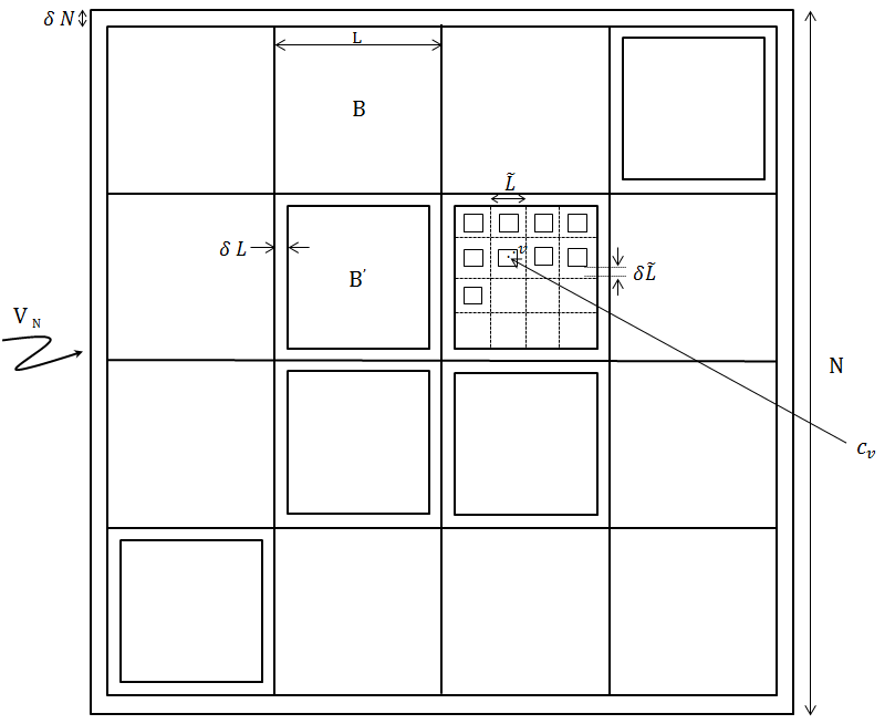
Figure 2: The boxes $B\in\mathcal{B}_{N}$, $B^{\prime}$, $\tilde{B}_{v,N}$

Throughout the paper, we will assume that $N=2^{n}$ for some $n\in\mathbb{Z}_{+}$. This does not affect the structure of the proof of Theorem 1.1, but substantially simplifies the notation in two ways. First, choosing $K$ so that $K$ divides $N$, it allows us to choose the boxes $V_{N}^{K,i}$ (defined at the beginning of the next section) to be of the same size; recall that $N\to\infty$ before $K\to\infty$. One can circumvent the assumption that $K$ divides $N$ by adjusting the size of the outer ring of boxes $V_{N}^{K,i}$ (see Figure 1); this will have no effect on the limit law because the probability that the maximum of $\eta_{v,N}$ lies in the outer ring of boxes tends to zero as $K\to\infty$. The assumption $N=2^{n}$ is also employed at the beginning of Section 4 in order to ensure that the length $L$ of the boxes $B$ defined there is divisible by $(1-\delta)N$, with $\delta>0$ fixed (see Figure 2). This restriction on $N$ is easily circumvented by adjusting slightly the width of the $\delta N$-strip along the perimeter of the box $V_{N}$ (so that both $K$ and $L$ divide $(1-\delta)N$, which allows general $N$); this again does not change the argument.

Notation. For functions $F(\cdot)$ and $G(\cdot)$, we write $F\lesssim G$ or $F=O(G)$ if there exists an absolute constant $C>0$ such that $F\leqslant CG$ everywhere in the domain. We write $F\asymp G$ if $F\lesssim G$ and $G\lesssim F$. For a parameter $\alpha$, we use $F\lesssim_{\alpha}G$ and $F\asymp_{\alpha}G$ if the constant $C$ above depends on the parameter $\alpha$. For a vector $x\in{\mathbb{R}}^{d}$, $[x]$ will denote the lattice point in ${\mathbb{Z}}^{d}$ whose coordinates are the integer parts of the corresponding coordinates of $x$.

2 The coarse and fine fields and the limit result

Let $\eta_{v,N}$ denote the GFF in the box $V_{N}$. As mentioned above, we assume for simplicity that $N=2^{n}$. Recall that $\eta_{N}^{*}=\max_{v\in V_{N}}\eta_{v,N}$. Fix $K=2^{k}$, with $k$ an integer. Tile the box $V_{N}$ with $4^{k}$ shifts of $V_{N/K}$, denoted by $V_{N}^{K,i}$, and let ${\cal F}={\cal F}_{N,K}$ denote the sigma-algebra generated by $\{\eta_{v,N}:v\in\cup_{i}\partial V_{N}^{K,i}\}$. (The boundaries of $V_{N}^{K,i}$ do in fact overlap.) We now define

$$X_{v}^{c}=X_{v,N,K}^{c}={\mathbb{E}}(\eta_{v,N}\mid{\cal F}_{N,K}),\quad X_{v}^{f}=X_{v,N,K}^{f}=\eta_{v,N}-X_{v}^{c}\,.$$ (2)

Note that $X_{v}^{f}$ vanishes on the boundaries of the boxes $V_{N}^{K,i}$, that the Gaussian fields $\{X^{f}\}$ and $\{X^{c}\}$ are independent, and that the fields $\{X_{v}^{f}\}_{v\in V_{N}^{K,i}}$ are independent for different $i$ and identically distributed as the GFF with zero boundary condition in $V_{N}^{K,i}$.

Throughout the argument, we will need to consider points that are within an appropriate distance from the boundary of the boxes $V_{N}^{K,i}$. Toward this end, fix $\delta>0$, with $1/\delta$ a power of $2$, and define the boxes

$$V_{N}^{K,\delta,i}=\{x\in V_{N}^{K,i}:d_{\infty}(x,\partial V_{N}^{k,i})\geqslant\delta N/K\}\,;$$ (3)

set

$$V^{K,\delta}_{N}=\cup_{i}V_{N}^{K,\delta,i}\,,\quad\Delta_{N}=\Delta_{N}^{K,\delta}=V_{N}\setminus V^{K,\delta}_{N}\,.$$

In addition, we write $V_{N}^{\delta}=V_{N}^{1,\delta}$. Note that $|\Delta_{N}|\leqslant{8}\delta|V_{N}|$.

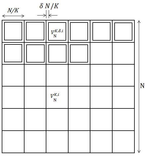
Figure 1: The boxes $V_{N}$, $V_{N}^{K,i}$, $V_{N}^{K,\delta,i}$

2.1 The coarse field limit

We describe in this short subsection the scaling limit of the Gaussian field $X^{c}_{\cdot,N,K}$. Introduce the covariance

$${\bf C}^{c}_{N,K}(v,v^{\prime})={\mathbb{E}}(X^{c}_{v,N,K}X^{c}_{v^{\prime},N,K})\,,\quad v,v^{\prime}\in V_{N}\,.$$ (4)

Consider the unit square $W=[0,1]^{2}$ and tile it with open squares $\{W^{i}\}_{i=1,\ldots,K^{2}}$ of side length $1/K$ each. (We omit $K$ from the notation.) Define $W^{\delta,i}$ to be the closed subset of $W^{i}$ consisting of points whose $\ell_{\infty}$-distance to the boundary of $W^{i}$ is at least $\delta/K$, and introduce the closed set $W^{\delta}=\cup_{i}W^{\delta,i}$. Note that when $N,K,1/\delta$ are all powers of $2$, we have $W^{\delta}=\mbox{\rm cl}(\{x/N:[x]\in V_{N}^{K,\delta}\})$; similarly, $W^{i}=\{x/N:[x]\in V_{N}^{K,i}\}^{o}$ and $W^{\delta,i}=\mbox{\rm cl}(\{x/N:[x]\in V_{N}^{K,\delta,i}\})$.

In what follows, we let $\{w_{t}\}_{t\geqslant 0}$ denote planar Brownian motion and we write $\mathbb{P}^{x}({\mathbb{E}}^{x})$ for probabilities (expectations) involving the path of $w_{t}$, with $w_{0}=x$. Set $\tau_{i}=\min\{t:w_{t}\in\partial W^{i}\}$ and $\tau=\min\{t:w_{t}\in\partial W\}$. Introduce the Poisson kernels $p(x,z)$ and $p_{i}(x,z)$ as the functions satisfying

$$\int_{\partial W}p(x,z)f(z)dz={\mathbb{E}}^{x}(f(w_{\tau}))\,,\quad\int_{\partial W^{i}}p_{i}(x,z)g(z)dz={\mathbb{E}}^{x}(g(w_{\tau_{i}}))\,,$$

for any continuous functions $f,g$, where $dz$ is one-dimensional Lebesgue measure. These Poisson kernels give the exit measures of Brownian motion from $W$ and $W^{i}$. For $x,x^{\prime}\in\cup_{\delta}W^{\delta}$, set

$${{\bf C}}^{c}_{K}(x,x^{\prime})=\left\{\begin{array}[]{ll}\frac{2}{\pi}\left(\int_{\partial W}p(x,z)\log|z-x^{\prime}|dz-\int_{\partial W^{i}}p(x,z)\log|z-x^{\prime}|dz\right)\,,&x,x^{\prime}\in W^{i}\,\mbox{\rm for some }i\\ \frac{2}{\pi}\left(\int_{\partial W}p(x,z)\log\left(\frac{|z-x^{\prime}|}{|x-x^{\prime}|}\right)dz\right)\,,&\mbox{\rm otherwise}\end{array}\right.\,.$$

Note that, for each fixed $\delta$, ${{\bf C}}^{c}_{K}$ is uniformly continuous on $W^{\delta}\times W^{\delta}$; in fact, it follows from the definition that for some constant $c_{\delta}>0$,

$$\sup_{x\in W^{\delta}}{{\bf C}}_{K}^{c}(x,x)\leqslant\frac{2}{\pi}\log K+c_{\delta}\,.$$ (5)

The following result is crucial for our approach and is easily verified.

Lemma 2.1.

Fix $\delta,K>0$. Then

$$\sup_{v,v^{\prime}\in(V_{N}^{K,\delta})^{2}}|{\bf C}^{c}_{N,K}(v,v^{\prime})-{\bf C}^{c}_{K}(v/N,v^{\prime}/N)|\to_{N\to\infty}0\,.$$ (6)

Note that the limit ${\bf C}^{c}_{K}$ depends on $K$ and that the convergence rate depends also on $\delta$.

Proof.

Employing the orthogonal representation $\eta_{v,N}=X_{v}^{c}+X_{v}^{f}$,

$${\mathbb{E}}(X_{v}^{c}X_{v^{\prime}}^{c})={\mathbb{E}}(\eta_{v,N}\eta_{v^{\prime},N})-{\mathbb{E}}(X_{v}^{f}X_{v^{\prime}}^{f})\,.$$ (7)

Recall that

$${\mathbb{E}}(\eta_{v,N}\eta_{v^{\prime},N})={\mathbb{E}}^{v}(\sum_{n=0}^{\tau_{N}}{\bf 1}_{\{S_{n}=v^{\prime}\}})\,,$$

where, under the measure ${\mathbb{E}}^{v}$, $\{S_{n}\}$ denotes two-dimensional simple random walk starting from $v$ and $\tau_{N}$ is the first exit time from $V_{N}$ (see [7] or [11]). Consider the potential kernel for two-dimensional simple random walk,

$$a(x)=\frac{2}{\pi}\log|x|+\frac{2\bar{\gamma}+\log 8}{\pi}+O(|x|^{-2})\,,$$ (8)

with $a(0)=0$, and where $\bar{\gamma}$ is the Euler constant (see [17, Theorem 4.4.4]). From [17, Theorem 4.6.2],

$${\mathbb{E}}(\eta_{v,N}\eta_{v^{\prime},N})={\mathbb{E}}^{v}(\sum_{n=0}^{\tau_{N}}{\bf 1}_{\{S_{n}=v^{\prime}\}})=\sum_{z\in\partial V_{N}}\mathbb{P}^{v}(S_{\tau_{N}}=z)a(z-v^{\prime})-a(v^{\prime}-v)\,.$$ (9)

Similarly, when $v,v^{\prime}\in V_{N}^{K,i}$ for some $i$,

$${\mathbb{E}}(X_{v}^{f}X_{v^{\prime}}^{f})=\sum_{z\in\partial V_{N}^{K,i}}\mathbb{P}^{v}(S_{\tau_{N}^{(i)}}=z)a(z-v^{\prime})-a(v^{\prime}-v)\,,$$ (10)

where $\tau_{N}^{i}$ denotes the first exit time from $V_{N}^{K,i}$. On the other hand, when $v,v^{\prime}$ do not belong to the same box $V_{N}^{K,i}$, ${\mathbb{E}}(X_{v}^{f}X_{v^{\prime}}^{f})=0$. The conclusion follows from the convergence of simple random walk to Brownian motion, the uniform continuity of $a(\cdot)$ on $\{z:\delta<|z|\leqslant 1\}$, (8), (9) and (10). ∎

It follows from Lemma 2.1 that ${\bf C}^{c}_{K}$ is a covariance function and therefore there exists a mean zero Gaussian field $\{Z^{c}_{K,\delta}(x)\}_{x\in W^{K,\delta}}$ with covariance ${\bf C}^{c}_{K}$.

2.2 The fine field limit

We fix a function $g(K)$ that grows to $\infty$ with $K$. (The choice $g(K)=\alpha\log\log K$, with an appropriately chosen $\alpha>0$, will be used in Proposition 5.2.) The following two propositions on the right tail behavior of $\max_{v}\eta_{N/K}$ will be demonstrated in Section 4. They will be important ingredients for the proof of Theorem 2.4 in several places in Section 6.

Proposition 2.2.

Define the event

$${\cal A}_{N,K}=\{\max_{v\in V_{N/K}}\eta_{v,N/K}\geqslant m_{N/K}+g(K)\}\,.$$

There exists an absolute constant $\alpha^{*}>0$ so that

$$\lim_{K\to\infty}\limsup_{N\to\infty}\frac{\mathrm{e}^{\sqrt{2\pi}g(K)}}{g(K)}\mathbb{P}({\cal A}_{N,K})=\lim_{K\to\infty}\liminf_{N\to\infty}\frac{\mathrm{e}^{\sqrt{2\pi}g(K)}}{g(K)}\mathbb{P}({\cal A}_{N,K})=\alpha^{*}\,.$$ (11)

Choose $v^{*}=v^{*}_{N/K}$ so that $\max_{v\in V_{N/K}}\eta_{v,N/K}=\eta_{v^{*},N/K}.$ There exists a continuous function $\psi:(0,1)^{2}\to(0,\infty)$, with $\int_{(0,1)^{2}}\psi(y)dy=1$, such that, for any open set $A\subset(0,1)^{2}$ and any sequence $x_{K}\geqslant 0$ not depending on $N$,

$$\lim_{K\to\infty}\limsup_{N\to\infty}\frac{\mathrm{e}^{\sqrt{2\pi}x_{K}}g(K)}{g(K)+x_{K}}\mathbb{P}(\max_{v\in V_{N/K}}\eta_{v,N/K}\geqslant m_{N/K}+g(K)+x_{K},Kv^{*}/N\in A|{\cal A}_{N,K})$$

$$=\lim_{K\to\infty}\liminf_{N\to\infty}\frac{\mathrm{e}^{\sqrt{2\pi}x_{K}}g(K)}{g(K)+x_{K}}\mathbb{P}(\max_{v\in V_{N/K}}\eta_{v,N/K}\geqslant m_{N/K}+g(K)+x_{K},Kv^{*}/N\in A|{\cal A}_{N,K})$$

$$=\int_{A}\psi(y)dy\,,$$ (12)

with convergence being uniform in the sequence $x_{K}$.

Fix $\delta>0$ small and recall that

$$V_{N}^{\delta}=\{x\in V_{N}:d_{\infty}(x,\partial V_{N})\geqslant\delta N\}\,.$$

Note that $V_{N}^{\delta}$ consists of the points in $V_{N}$ which are at distance at least $\delta N$ from the boundary of $V_{N}$; in particular, $V_{N}^{\delta}$ is not the rescaled version of $W^{\delta}$. In the construction of the limit process, we will need a version of Proposition 2.2 that restricts attention to $V_{N/K}^{\delta}$.

Proposition 2.3.

Fix $\delta>0$ small and let $\alpha^{*},\psi$ be as in Proposition 2.2. Set $m_{\delta}=\int_{(\delta,1-\delta)^{2}}\psi(y)dy$ and $\psi^{\delta}=\psi/m_{\delta}$. Define the event

$${\cal A}_{N,K,\delta}=\{\max_{v\in V_{N/K}^{\delta}}\eta_{v,N/K}\geqslant m_{N/K}+g(K)\}\,.$$

Then

$$\lim_{K\to\infty}\lim_{N\to\infty}\frac{\mathrm{e}^{\sqrt{2\pi}g(K)}}{g(K)}\mathbb{P}({\cal A}_{N,K})=\alpha^{*}m_{\delta}\,.$$ (13)

Choose $v^{*}_{\delta}=v^{*}_{N/K,\delta}$ so that $\max_{v\in V_{N/K}^{\delta}}\eta_{v,N/K}=\eta_{v^{*}_{\delta},N/K}$. For any open set $A\subset(\delta,1-\delta)^{2}$ and any sequence $x_{K}\geqslant 0$ not depending on $N$,

$$\lim_{K\to\infty}\lim_{N\to\infty}\frac{\mathrm{e}^{\sqrt{2\pi}x_{K}}g(K)}{g(K)+x_{K}}\mathbb{P}(\max_{v\in V_{N/K}^{\delta}}\eta_{v,N/K}\geqslant m_{N/K}+g(K)+x_{K},Kv^{*}_{\delta}/N\in A|{\cal A}_{N,K,\delta})=\int_{A}\psi^{\delta}(y)dy\,,$$ (14)

with convergence being uniform in the sequence $x_{K}$.

2.3 The limit process

Let $\psi^{\delta}$ and $\alpha^{*}$ be as in Proposition 2.3. In each $W^{\delta,i}$, choose a point $z_{i}^{K,\delta}$ that is distributed according to the scaled analog of $\psi^{\delta}$, with $z_{i}^{K,\delta}$ being chosen independently for different $i$. Let $\{{\wp}_{i}^{K,\delta}\}_{i=1,\ldots,K^{2}}$ denote independent Bernoulli random variables with $\mathbb{P}({\wp}_{i}^{K,\delta}=1)=\alpha^{*}m_{\delta}g(K)\mathrm{e}^{-\sqrt{2\pi}g(K)}$, and let $\{Y_{i}^{K}\}_{i=1,\ldots,K^{2}}$ denote independent random variables satisfying

$$\mathbb{P}(Y_{i}^{K}\geqslant x)=\frac{g(K)+x}{g(K)}\mathrm{e}^{-\sqrt{2\pi}x}\,,\quad x\geqslant 0\,.$$ (15)

Recall the limiting coarse field $Z^{c}_{K,\delta}$ and define

$$G_{i}^{K,\delta}={\wp}_{i}^{K}(Y_{i}^{K}+g(K))+Z^{c}_{K,\delta}(z_{i}^{K,\delta})-2\sqrt{2/\pi}\log K.$$

Set $G^{*}_{K,\delta}=\max_{i}G_{i}^{K,\delta}$ and denote by $\mu_{K,\delta}$ its law. Note that $\mu_{K,\delta}$ does not depend on $N$.

Let $d(\cdot,\cdot)$ denote the Lévy metric, which is compatible with the weak convergence of probability measures on ${\mathbb{R}}$. Our main result in the paper is the following.

Theorem 2.4.

Let $\mu_{N}$ denote the law of $\max_{v\in V_{N}}\eta_{v}^{N}-m_{N}$. Then, with $\mu_{K,\delta}$ defined as above,

$$\lim_{\delta\searrow 0}\limsup_{K\to\infty}\limsup_{N\to\infty}d(\mu_{N},\mu_{K,\delta})=0\,.$$ (16)

In particular, there exists a probability measure $\mu_{\infty}$ on ${\mathbb{R}}$ such that $d(\mu_{N},\mu_{\infty})\to_{N\to\infty}0$.

(The choice of working with the Lévy metric in Theorem 2.4 is for concreteness; any distance compatible with weak convergence could be used.) The limit $\mu_{\infty}$ in Theorem 2.4 can be described as follows. A similar description was derived in [3].

Theorem 2.5.

There exist a random variable $Z>0$ and a constant $\alpha^{*}>0$ so that

$$\mu_{\infty}\left((-\infty,x]\right)={\mathbb{E}}\left(e^{-\alpha^{*}Ze^{-\sqrt{2\pi}x}}\right)\,.$$ (17)

Thus, the limit law of the maximum of the GFF is a randomly shifted Gumbel distribution. (In the statement of Theorem 2.5, the constant $\alpha^{*}$ can be absorbed into $Z$. Since $\alpha^{*}$ is determined by the tail behavior of the GFF (see Proposition 4.1) whereas the random variable $Z$ is determined by the coarse field, they play very different roles in the proof; for this reason, we keep both in the statement.) Note that the random variable $Z$ plays the role of the derivative martingale in the theory of branching Brownian motion, as in [16].

3 Preliminaries

3.1 Branching random walk and modified branching random walk

We first briefly review the construction of branching random walk (BRW) and modified branching random walk (MBRW), which we construct so as to simplify comparisons with the GFF. As before, we let $V_{N}$ denote the box of side length $N$ intersected with $\mathbb{Z}^{2}$ such that the lower left corner is at the origin, and set $n=\log_{2}N$. For $j\in[0,\ldots,n-1]$, let $\mathfrak{B}_{j}$ be the collection of squared boxes in $\mathbb{Z}^{2}$ of side length $2^{j}$ with corners in $\mathbb{Z}^{2}$, and let $\mathfrak{BD}_{j}$ denote the subset of $\mathfrak{B}_{j}$ consisting of squares of the form $([0,2^{j}-1]\cap\mathbb{Z})^{2}+(i_{1}2^{j},i_{2}2^{j})$, with $i_{1},i_{2}\in\mathbb{N}$. For $v\in\mathbb{Z}^{2}$, let $\mathfrak{B}_{j}(v)=\{B\in\mathfrak{B}_{j}:v\in B\}$ be the collection of boxes in $\mathfrak{B}_{j}$ that contain $v$, and define $\mathfrak{BD}_{j}(v)$ to be the (unique) box in $\mathfrak{BD}_{j}$ that contains $v$. Furthermore, denote by $\mathfrak{B}_{N,j}$ the subset of $\mathfrak{B}_{j}$ consisting of boxes whose lower left corners are in $V_{N}$. Let $\{\bar{\phi}_{N,j,B}\}_{j\geqslant 0,B\in\mathcal{BD}_{j}}$ be i.i.d. mean zero Gaussian variables with variance $\frac{2\log 2}{\pi}$, and define a branching random walk

$$\vartheta_{v,N}=\mbox{$\sum_{j=0}^{n-1}$}\bar{\phi}_{N,j,\mathcal{BD}_{j}(v)}\,.$$ (18)

For $j\in[0,\ldots,n-1]$ and $B\in\mathfrak{B}_{N,j}$, let $\phi_{N,j,B}$ be independent mean zero Gaussian variables with $\operatorname{Var}(\phi_{N,j,B})=\tfrac{2\log 2}{\pi}\cdot 2^{-2j}$, and define

$$\phi_{N,j,B}=\phi_{N,j,B^{\prime}},\mbox{ for }B\sim_{N}B^{\prime}\in\mathcal{B}_{N,j}\,,$$ (19)

where $B\sim_{N}B^{\prime}$ if and only if there exist $i_{1},i_{2}\in\mathbb{Z}$ such that $B=(i_{1}N,i_{2}N)+B^{\prime}$. (Note that, for any $B\in\mathcal{B}_{j}$, there exists a unique $B^{\prime}\in\mathfrak{B}_{N,j}$ such that $B\sim_{N}B^{\prime}$.) Let $d_{N}(u,v)=\min_{w\sim_{N}v}|u-w|$ be the $\ell^{2}$ distance between $u$ and $v$ when considering $V_{N}$ as a torus, for all $u,v\in V_{N}$. Finally, we define the MBRW $\{\xi_{v,N}:v\in V_{N}\}$ by

$$\xi_{v,N}=\mbox{$\sum_{j=0}^{n-1}\sum_{B\in\mathfrak{B}_{j}(v)}$}\phi_{N,j,B}\,.$$ (20)

The motivation for introducing MBRW is that the MBRW approximates the GFF with high precision. That is, the covariance structure of the MBRW approximates that of the GFF well. This is elaborated in the next lemma.

Lemma 3.1.

For any $0<\delta<1/100$, there exists a constant $C=C_{\delta}$ such that, for all $n$,

$$|\mathrm{Cov}(\xi_{u,N},\xi_{v,N})-\tfrac{2\log 2}{\pi}(n-\log_{2}(d_{N}(u,v)))| \leqslant C,\mbox{ for all }u,v\in V_{N}\,,$$

$$\big{|}\mathrm{Cov}(\eta_{u,N},\eta_{v,N})-\tfrac{2\log 2}{\pi}(n-(0\vee\log_{2}|u-v|))\big{|} \leqslant C,\mbox{ for all }u,v\in V^{\prime}_{N}\,,$$

where $V^{\prime}_{N}$ is a box of side length $(1-2\delta)N$ placed at the center of $V_{N}$.

The first part of the lemma is in [7, Lemma 2.2], whereas the second part can be found in [9, Lemma 2.1] (and in a slightly different form, dealing with the so called torus GFF, in [7, Lemma 2.2]).

3.2 A few Gaussian inequalities

We will need the following two Gaussian comparison inequalities: the Sudakov-Fernique inequality, which compares the expected maximum of Gaussian processes (see, e.g., [13] for a proof), and Slepian’s comparison lemma [21], which compares the maximum of Gaussian processes in the sense of “stochastic domination”.

Lemma 3.2 (Sudakov-Fernique).

Let $\mathcal{A}$ be an arbitrary finite index set and let $\{X_{a}\}_{a\in\mathcal{A}}$ and $\{Y_{a}\}_{a\in\mathcal{A}}$ be two centered Gaussian processes such that

$${\mathbb{E}}(X_{a}-X_{b})^{2}\geqslant{\mathbb{E}}(Y_{a}-Y_{b})^{2}\,,\mbox{ for all }a,b\in\mathcal{A}\,.$$ (21)

Then ${\mathbb{E}}\max_{a\in\mathcal{A}}X_{a}\geqslant{\mathbb{E}}\max_{a\in\mathcal{A}}Y_{a}$.

Lemma 3.3 (Slepian).

Let $\mathcal{A}$ be an arbitrary finite index set and let $\{X_{a}\}_{a\in\mathcal{A}}$ and $\{Y_{a}\}_{a\in\mathcal{A}}$ be two centered Gaussian processes such that (21) holds and $\operatorname{Var}X_{a}=\operatorname{Var}Y_{a}$ for all $a\in\mathcal{A}$. Then $\mathbb{P}(\max_{a\in\mathcal{A}}X_{a}\geqslant\lambda)\geqslant\mathbb{P}(\max_{a\in\mathcal{A}}Y_{a}\geqslant\lambda)$, for all $\lambda\in\mathbb{R}$.

The following Borell-Tsirelson inequality is a central result in the theory of concentration of measure; see, for example, [19, Theorem 7.1, Equation (7.4)].

Lemma 3.4.

Consider a Gaussian process $\{\eta_{x}:x\in\mathcal{A}\}$, with $\mathcal{A}$ finite, and set $\sigma=\sup_{x\in\mathcal{A}}({\mathbb{E}}(\eta_{x}^{2}))^{1/2}$. Then, for $\alpha>0$,

$$\mathbb{P}\left(\left|\max_{x\in\mathcal{A}}\eta_{x}-{\mathbb{E}}\,\max_{x\in\mathcal{A}}\eta_{x}\right|>\alpha\right)\leqslant 2\exp(-\alpha^{2}/2\sigma^{2})\,.$$

We will often need to control the expectation of the maximum of a Gaussian field in terms of its covariance structure. This is achieved by Fernique’s criterion [13]. We quote a version suited to our needs, which follows straightforwardly from the version in [2, Theorem 4.1] by using, as the majorizing measure, the normalized counting measure on $B$.

Lemma 3.5.

There exists a universal constant $C_{F}>0$ with the following property. Let $B\subset\mathbb{Z}^{2}$ denote a (discrete) box of side length $b$ and assume $\{G_{v}\}_{v\in B}$ is a mean zero Gaussian field satisfying

$${\mathbb{E}}(G_{v}-G_{u})^{2}\leqslant|u-v|/b\,,\mbox{ for all }u,v\in B\,.$$

Then

$${\mathbb{E}}\max_{v\in B}G_{v}\leqslant C_{F}\,.$$ (22)

3.3 A Brownian motion estimate

In (24), we show that the probabilities for Brownian motion to stay below two close curves are asymptotically the same and, in (25) and (26), we give bounds on the corresponding probabilities. In Section 4, the asymptotic probabilities, as $N\rightarrow\infty$, of the events in (82) will be strongly tied to these bounds.

Lemma 3.6.

Let $C\geqslant 0$ be a fixed absolute constant, and let $\{W_{s}:s\geqslant 0\}$ be a mean zero Brownian motion, started at $0$, with variance $\sigma^{2}s$, $\sigma>0$, at time $s$. For $y>1$ and $t>0$, define densities $\mu_{t,y}(\cdot)$ and $\mu_{t,y}^{*}(\cdot)$ such that, for all intervals $I$,

$$\begin{split}\mathbb{P}&(W_{t}\in I;W_{s}\leqslant y\mbox{ for all }0\leqslant s\leqslant t)=\int_{I}\mu_{t,y}(x)dx\,,\\ \mathbb{P}&(W_{t}\in I;W_{s}\leqslant y+y^{1/20}+C(s\wedge(t-s))^{1/20}\mbox{ for all }0\leqslant s\leqslant t)=\int_{I}\mu^{*}_{t,y}(x)dx\,.\end{split}$$ (23)

Then there exists $\delta_{y}$, with $\delta_{y}\searrow_{y\to\infty}0$, such that, for all $x\leqslant 0$ and $t>0$,

$$\mu_{t,y}^{*}(x)\leqslant(1+\delta_{y})\mu_{t,y}(x)\,.$$ (24)

For all $x\leqslant y+y^{1/20}$,

$$\mu^{*}_{t,y}(x)\lesssim y(y+y^{1/20}-x)t^{-3/2}e^{-x^{2}/2t\sigma^{2}}\,.$$ (25)

Furthermore,

$$\frac{\mu^{*}_{t,y}(x_{1})}{\mu^{*}_{t,y}(x_{2})}\leqslant\mathrm{e}^{-\frac{x_{1}^{2}-x_{2}^{2}}{2t\sigma^{2}}}\mbox{ for all }0\leqslant x_{2}\leqslant x_{1}\leqslant y+y^{1/20}\,.$$ (26)

Note that by setting $C=0$ and $\bar{y}=y+y^{1/20}$, (26) also implies that

$$\frac{\mu_{t,\bar{y}}(x_{1})}{\mu_{t,\bar{y}}(x_{2})}\leqslant\mathrm{e}^{-\frac{x_{1}^{2}-x_{2}^{2}}{2t\sigma^{2}}}\mbox{ for all }0\leqslant x_{2}\leqslant x_{1}\leqslant\bar{y}\,.$$ (27)

Proof of Lemma 3.6.

In order to show (26), note that $\{W_{s}-sW_{t}/t:0\leqslant s\leqslant t\}$ is distributed as a Brownian bridge that is independent of the value $W_{t}$. So, the probability that the Brownian motion $\{W_{s}:0\leqslant s\leqslant t\}$ stays below a given curve, after conditioning on $W_{t}=x$, is decreasing with $x$. Combined with the fact that $\mu^{*}_{t,y}(x)>0$ for all $x\leqslant y+y^{1/20}$, this implies the ratio between $\mu^{*}_{t,y}(x_{1})$ and $\mu^{*}_{t,y}(x_{2})$ is bounded above by the ratio of the densities for the Brownian motion at $x_{1}$ and $x_{2}$.

We next prove (24). By the reflection principle, for all $w\geqslant 0$,

$$\mu_{t,y}(y-w)=\frac{1}{\sqrt{2\pi t}\sigma}(\mathrm{e}^{-\frac{(w-y)^{2}}{2t\sigma^{2}}}-\mathrm{e}^{-\frac{(w+y)^{2}}{2t\sigma^{2}}}).$$ (28)

Let $\tau$ be a global maximizer of $\{W_{s}:0\leqslant s\leqslant t\}$, i.e., $W_{\tau}=\max_{0\leqslant s\leqslant t}W_{s}$, and write $\psi_{t,y}(s)=y+y^{1/20}+C(s\wedge(t-s))^{1/20}$ and $\psi_{t,y}^{*}(j)=\max_{s\in[j,j+1]}\psi_{t,y}(s)$. Summing over different $j$ for $\tau\in[j,j+1]$ and integrating over locations for $W_{j}$, we obtain from the Markov property applied at time $j$ and then again at time $\min\{s\geqslant j:W_{s}\geqslant y\}\wedge(j+1)$ that, for all $x\leqslant 0$,

$$\mu_{t,y}^{*}(x)-\mu_{t,y}(x)$$

$$\leqslant\sum_{j=0}^{\lfloor t\rfloor}\int_{-\infty}^{\psi_{t,y}^{*}(j)}\mu_{j,\psi_{t,y}^{*}(j)}(\lambda)\mathbb{P}(\lambda+\max_{0\leqslant s\leqslant 1}W_{s}\geqslant y)\max_{j\leqslant s\leqslant j+1}\,\max_{y\leqslant y^{\prime}\leqslant\psi_{t,y}^{*}(j)}\mu_{t-s,\psi_{t,y}^{*}(j)-y^{\prime}}(x-y^{\prime})d\lambda\,.$$

In the preceding inequality, the sum over $j$ corresponds to the intervals $[j,j+1)$, with the Brownian motion achieving its maximum at $\tau\in[j,j+1).$ (Note that, on the relevant event, $y\leqslant W_{\tau}\leqslant\psi_{t,y}(\tau)$, integration over $\lambda$ includes all possible locations of the Brownian motion at time $j$; the term $\mathbb{P}(\lambda+\max_{0\leqslant s\leqslant 1}W_{s}\geqslant y)$ bounds the probability for the Brownian motion to hit $y$ (i.e., $W_{\tau}\geqslant y$) given its location at time $j$; and the term $\max_{y\leqslant y^{\prime}\leqslant\psi_{t,y}^{*}(j)}\mu_{t-s,\psi_{t,y}^{*}(j)-y^{\prime}}(x-y^{\prime})$ bounds the probability for the Brownian motion to stay below $W(\tau)$ over the time interval $(\tau,t]$.) By (27), $\max_{y\leqslant y^{\prime}\leqslant\psi_{t,y}^{*}}\mu_{t-s,\psi_{t,y}^{*}(j)-y^{\prime}}(x-y^{\prime})\leqslant\mu_{t-s,\psi_{t,y}^{*}(j)-y}(x-y)$. Therefore,

$$\mu_{t,y}^{*}(x)-\mu_{t,y}(x) \lesssim\sum_{j=0}^{\lfloor t\rfloor}\int_{-\infty}^{\psi_{t,y}^{*}(j)}\mu_{j,\psi_{t,y}^{*}(j)}(\lambda)\mathrm{e}^{-\frac{(\lambda-y)_{-}^{2}}{2\sigma^{2}}}\max_{j\leqslant s\leqslant j+1}\mu_{t-s,\psi_{t,y}^{*}(j)-y}(x-y)d\lambda=:\sum_{j=0}^{\lfloor t\rfloor}\Phi_{j}\,,$$ (29)

where $(\lambda-y)_{-}=\mathbf{1}_{\lambda\leqslant y}|\lambda-y|$. Applying (28), we obtain that, for both $j\leqslant y^{2}/(\log y)^{2}$ and $j\geqslant t-y^{2}/(\log y)^{2}$,

$$\Phi_{j}\lesssim\mathrm{e}^{-(\log y)^{2}/4\sigma^{2}}(y-x)t^{-3/2}\,.$$ (30)

Again, by the reflection principle, for all $\lambda\leqslant\psi_{t,y}^{*}(j)$, $x\leqslant 0$ and $j-1\leqslant s\leqslant j$,

$$\mu_{j,\psi_{t,y}^{*}(j)}(\lambda) \lesssim j^{-3/2}(\psi_{t,y}^{*}(j)-\lambda)\psi_{t,y}^{*}(j)$$

$$\mu_{t-s,\psi_{t,y}^{*}(j)-y}(x-y) \lesssim(\psi_{t,y}^{*}(j)-y)(\psi_{t,y}^{*}(j)-x)(t-j)^{-3/2}\,.$$

For $y^{2}/(\log y)^{2}\leqslant j\leqslant t-y^{2}/(\log y)^{2}$, plugging the above estimates into the integral in (29) leads to

$$\Phi_{j} \lesssim(\psi_{t,y}^{*}(j)-y)^{3}j^{-3/2}(t-j)^{-3/2}(\psi_{t,y}^{*}(j)-x)\psi_{t,y}^{*}(j)\,.$$ (31)

Plugging (30) and (31) into (29) and summing over $j$, we obtain

$$\mu_{t,y}^{*}(x)-\mu_{t,y}(x)\lesssim(y-x)yt^{-3/2}(y^{2}\mathrm{e}^{-\frac{(\log y)^{2}}{4\sigma^{2}}}+y^{-1/2}\log y)\lesssim\mu_{t,y}(x)(y^{2}\mathrm{e}^{-\frac{(\log y)^{2}}{4\sigma^{2}}}+y^{-1/2}\log y)\,,$$

which completes the proof of (24) (where we have used $\mu_{t,y}(x)\asymp y(y-x)t^{-3/2}$).

It remains to show (25). The result follows by using the same decomposition for the location of the global maximizer $\tau$ of Brownian motion in a manner analogous to the proof of (24), together with similar straightforward computations. We omit further details. ∎

3.4 Refined estimates on the right tail of the maximum for the GFF

In [11], it is shown that

$$\mathbb{P}(\eta^{*}_{N}>m_{N}+\lambda)\asymp\lambda\mathrm{e}^{-\sqrt{2\pi}\lambda}\mbox{ for all }1\leqslant\lambda\leqslant\sqrt{\log N}\,.$$ (32)

In this subsection, we give a preliminary upper bound on the right tail of the maximum of GFF over subsets of $V_{N}$, for values of $\lambda$ that include $\lambda\gg\sqrt{\log N}$. To do this, we first obtain an upper bound on the probability of BRW taking atypically large values. We will use the notation of Subsection 3.1 and, for convenience, will view each $\vartheta_{v,N}$ as the value at time $n=\log_{2}N$ of a mean zero Brownian motion $\{\vartheta_{v,N}(t):0\leqslant t\leqslant n\}$ with variance rate $\frac{2\log 2}{\pi}$. More precisely, we associate to each Gaussian variable $\bar{\phi}_{N,j,B}$ an independent Brownian motion with variance rate $\frac{2\log 2}{\pi}$ that runs for one unit of time and ends at the value $\bar{\phi}_{N,j,B}$, with

$$\vartheta_{v,N}(t):=\sum_{j=0}^{[t]}\bar{\phi}_{N,j,\mathcal{BD}_{j}(v)}+\bar{\phi}_{N,j,\mathcal{BD}_{j}(v)}(t-[t])\,.$$

For $\beta>0$, define

$$G_{N}(\beta) =\bigcup_{v\in V_{N}}\bigcup_{0\leqslant t\leqslant n}\{\vartheta_{v,N}(t)\geqslant\beta+1+\frac{m_{N}}{n}t+10(\log(t\wedge(n-t)))_{+}\}\,.$$ (33)

Lemma 3.7.

There exists an absolute constant $C>0$ such that $\mathbb{P}(G_{N}(\beta))\lesssim(\beta\vee 1)\mathrm{e}^{-\sqrt{2\pi}\beta}\mathrm{e}^{-\beta^{2}/Cn}$ for all $\beta>0$.

Proof.

We may assume that $\beta>\beta_{0}$, for some $\beta_{0}>0$ large. For any $v\in V_{N}$, write $\bar{\vartheta}_{v,N}(t)=\vartheta_{v,N}(t)-\tfrac{m_{N}t}{n}$. For $j=1,\ldots,n$, define the probability measure $\mathbb{Q}_{j}$ by

$$\frac{d\mathbb{Q}_{j}}{d\mathbb{P}}=\mathrm{e}^{\tfrac{\pi m_{N}}{(2\log 2)n}\bar{\vartheta}_{v,N}(j)+\tfrac{\pi m_{N}^{2}}{(4\log 2)n}\cdot\tfrac{j}{n}}\,.$$ (34)

For $j=n$, we omit the subscript $j$ from the notation. Then, under $\mathbb{Q}_{j}$, $\{\bar{\vartheta}_{v,N}(t):0\leqslant t\leqslant j\}$ is a mean zero Brownian motion with variance rate $\frac{2\log 2}{\pi}$. We write $\frac{d\mathbb{Q}_{j}}{d\mathbb{P}}(x)$ for the expression in (34) when $\bar{\vartheta}_{v,N}(j)=x$.

For $0\leqslant t\leqslant n$, write $\psi_{N,t,\beta}=\beta+1+10(\log(t\wedge(n-t)))_{+}$. For $j\in[1,\ldots,n]$, let $\chi_{N,j}(\cdot)$ be the density function such that, for all $I\subseteq\mathbb{R}$,

$$\mathbb{P}(\bar{\vartheta}_{v,N}(t)\leqslant\psi_{N,t,\beta}\mbox{ for all }t\leqslant j,\bar{\vartheta}_{v,N}(j)\in I)=\int_{I}\chi_{N,j}(x)dx\,.$$

By a straightforward union bound,

$$\mathbb{P}(G_{N}(\beta)) \leqslant\sum_{j=1}^{n-1}4^{j+1}\int_{-\infty}^{\psi_{N,j,\beta}}\chi_{N,j}(x)\mathbb{P}({\exists s\in[0,1]:x+\gamma W(s)\geqslant\psi_{N,s,\beta}})dx$$

$$\quad+4\mathbb{P}(\exists s\in[0,1]:\bar{\vartheta}_{v,N}(s)\geqslant\psi_{N,s,\beta})\,,$$ (35)

where $\{W_{s}:0\leqslant s\leqslant 1\}$ is an independent Brownian motion and $\gamma=\sqrt{2\log 2}$. Applying (25) (with $j$ in place of $t$ and $\psi_{N,j,\beta}$ in place of $y+y^{1/20}$), we see that, for $x\leqslant\psi_{N,j,\beta}$ and $j\geqslant 1$,

$$(\frac{d\mathbb{P}}{d\mathbb{Q}_{j}}(x))^{-1}\chi_{N,j}(x)\lesssim j^{-3/2}\psi_{N,j,\beta}(\psi_{N,j,\beta}-x)e^{-\pi x^{2}/4j\log 2}\,.$$ (36)

Combined with (34) and using that $(j/n)\log n\leqslant\log j$, this yields

$$\chi_{N,j}(x)\lesssim 4^{-j}\mathrm{e}^{-(\sqrt{2\pi}-O((\log n)/n))x}\mathrm{e}^{-\pi x^{2}/4j\log 2}\psi_{N,j,\beta}(\psi_{N,j,\beta}-x)\,.$$ (37)

On the other hand,

$$\mathbb{P}(\exists s\in[0,1]:x+\gamma W(s)\geqslant\psi_{N,s,\beta})\lesssim\exp(-(\min_{s\in[j,j+1]}\psi_{N,s,\beta}-x)^{2}/(2\gamma^{2}))\,.$$ (38)

Since the right hand side of (38) decays (essentially) exponentially in $|\psi_{N,j,\beta}-x|^{2}$, the typical value of $x$ that will contribute to the integral of (3.4) will be close to $\psi_{N,j,\beta}$. With this observation in mind, plugging (38) and (37) into (3.4), we obtain that, for an absolute constant $C>0$,

$$\mathbb{P}(G_{N}(\beta)) \lesssim\sum_{j=1}^{n}(\beta\vee 1)4^{j}4^{-j}(j\wedge(n+1-j))^{-2}\mathrm{e}^{-\sqrt{2\pi}\beta}\mathrm{e}^{-\beta^{2}/Cn}\lesssim(\beta\vee 1)\mathrm{e}^{-\sqrt{2\pi}\beta}\mathrm{e}^{-\beta^{2}/Cn}\,,$$

where the power 2 in $(j\wedge(n+1-j))^{2}$ is obtained from the slackness term $10(\log(j\wedge(n-j)))_{+}$ (with room to spare). ∎

Lemma 3.8.

There exist absolute constants $C,C^{\prime}>0$ such that, for all $N\in\mathbb{N}$ and $z\geqslant 1$,

$$\mathbb{P}(\max_{v\in V_{N}}\eta_{v,N}\geqslant m_{N}+z)\leqslant C^{\prime}z\mathrm{e}^{-\sqrt{2\pi}z}\mathrm{e}^{-C^{-1}z^{2}/n}\,.$$ (39)

Furthermore,

$$\mathbb{P}(\max_{v\in A}\eta_{v,N}\geqslant m_{N}+z-y)\lesssim(\frac{|A|}{|V_{N}|})^{1/2}z\mathrm{e}^{-\sqrt{2\pi}(z-y)}\mbox{ for all }z\geqslant 1,y\geqslant 0\,,$$ (40)

for all $A\subseteq V_{N}$.

Proof.

By the same argument as in [11, Lemma 2.6], for an absolute constant $\kappa\geqslant 0$ and any $A\subseteq V_{N}$,

$$\mathbb{P}(\max_{v\in A}\eta_{v,N}\geqslant\lambda)\leqslant\mathbb{P}(\max_{v\in 2^{\kappa}A}\vartheta_{v,2^{\kappa}N}\geqslant\lambda)\mbox{ for all }\lambda\in\mathbb{R}\,,$$

where $\{\vartheta_{v,2^{\kappa}N}\}$ is a BRW on 2D box of side length $2^{\kappa}N$. By this inequality and a change of variable (replacing $2^{\kappa}N$ by $N$), it suffices to prove (39) and (40) for BRW. For $\beta>0$, define

$$F_{v,N}(\beta,z) =\{\vartheta_{v,N}(t)\leqslant\beta+1+\frac{m_{N}}{n}t+10\log(t\wedge(n-t))_{+}\mbox{ for all }0\leqslant t\leqslant n;\vartheta_{v,N}\geqslant m_{N}+z\}\,.$$

We first prove the BRW version for (39), using the notation $\mu_{n,z}(\cdot)$ and $\mu^{*}_{n,z}(\cdot)$ from (23) (with variance rate $\sigma^{2}=\frac{2\log 2}{\pi}$). By (25), and using $d\mathbb{P}/d\mathbb{Q}$ as in Lemma 3.7 (with $z^{\prime}$ satisfying $z^{\prime}+(z^{\prime})^{1/20}=z+1$),

$$\mathbb{P}(F_{v,N}(z,z)) =\int_{z}^{z+1}\frac{d\mathbb{P}}{d\mathbb{Q}}(x+m_{N})\mu^{*}_{n,z^{\prime}}(x)dx$$

$$\leqslant\int_{z}^{z+1}4^{-n}n^{3/2}\mathrm{e}^{-(\sqrt{2\pi}-O((\log n)/n))x}\mathrm{e}^{-\pi z^{2}/4n\log 2}\cdot zn^{-3/2}dx$$

$$\lesssim 4^{-n}z\mathrm{e}^{-\sqrt{2\pi}z}\mathrm{e}^{-\pi z^{2}/4n\log 2}\mathrm{e}^{O((\log n)/n)z}\,.$$ (41)

Inequality (39) follows by summing the above inequality over $v\in V_{N}$ and applying Lemma 3.7.

We next demonstrate (40). First note that, if $z-y+(|V_{N}|/|A|)^{1/4}\leqslant 1$, then (40) holds automatically. We next consider the case when $z-y+(|V_{N}|/|A|)^{1/4}\geqslant 1$ and set $\beta=z-y+(|V_{N}|/|A|)^{1/4}$. By Lemma 3.7,

$$\mathbb{P}(G_{N}(\beta))\lesssim(\beta\vee 1)\mathrm{e}^{-\sqrt{2\pi}(z-y)}\mathrm{e}^{-\sqrt{2\pi}(|V_{N}|/|A|)^{1/4}}\,.$$ (42)

Analogous to the derivation of (41), we obtain

$$\mathbb{P}(F_{v,N}(\beta,z-y))\lesssim 4^{-n}(\beta\vee 1)(|V_{N}|/|A|)^{1/4}\mathrm{e}^{-\sqrt{2\pi}(z-y)}\,.$$

Therefore, we get that

$$\mathbb{P}(\max_{v\in A}\eta_{v,N}\geqslant m_{N}+z-y)\lesssim\mathbb{P}(G_{N}(\beta))+\sum_{v\in A}\mathbb{P}(F_{v,N}(\beta,z-y))\lesssim(\frac{|A|}{|V_{N}|})^{1/2}z\mathrm{e}^{-\sqrt{2\pi}(z-y)}\,,$$

where we have used the facts that $\beta\leqslant 2z(|V_{N}|/|A|)^{1/4}$ and $|V_{N}|=4^{n}$. This completes the verification of (40). ∎

3.5 Robustness of the maximum for the GFF

The following lemma shows a form of robustness for the maximum of the GFF under perturbation.

Lemma 3.9.

Let $\phi_{u,N}$ be independent variables such that, for all $u\in V_{N}$ and $y\geqslant 0$,

$$\mathbb{P}(\phi_{u,N}\geqslant 1+y)\leqslant\mathrm{e}^{-y^{2}}\,.$$

There exist absolute constants $c,C>0$ such that, for any $\varepsilon>0$, $N\in\mathbb{N}$ and $-c\varepsilon^{-1/2}\leqslant x\leqslant\sqrt{\log N}$,

$$\mathbb{P}(\max_{u\in V_{N}}(\eta_{u,N}+\varepsilon\phi_{u,N})\geqslant m_{N}+x)\leqslant\mathbb{P}(\max_{u\in V_{N}}\eta_{u,N}\geqslant m_{N}+x-\sqrt{\varepsilon})(1+O(\mathrm{e}^{-C^{-1}\varepsilon^{-1}}))\,.$$ (43)

Furthermore, ${\mathbb{E}}\max_{u\in V_{N}}(\eta_{u,N}+\varepsilon\phi_{u,N})\leqslant{\mathbb{E}}\max_{u\in V_{N}}\eta_{u,N}+C\sqrt{\varepsilon}+C\varepsilon^{2}\mathbf{1}_{\varepsilon\geqslant 1}$.

Proof.

Consider first the case $\varepsilon\leqslant 1$. Setting $\Gamma_{y}=\{u\in V_{N}:y/2\leqslant\varepsilon\phi_{u,N}\leqslant y\}$, we have

$$\mathbb{P}(\max_{u\in V_{N}}(\eta_{u,N}+\varepsilon\phi_{u,N})\geqslant m_{N}+x) \leqslant\mathbb{P}(\max_{u\in V_{N}}\eta_{u,N}\geqslant m_{N}+x-\sqrt{\varepsilon})$$

$$\qquad+\sum_{i=0}^{\infty}{\mathbb{E}}(\mathbb{P}(\max_{u\in\Gamma_{2^{i}\sqrt{\varepsilon}}}\eta_{u,N}\geqslant m_{N}+x-2^{i}\sqrt{\varepsilon}\mid\Gamma_{2^{i}\sqrt{\varepsilon}})),\,$$ (44)

where the conditioning on the right side of the last display means conditioning on the locations of points $u\in V_{N}$ where the random field $\phi_{u,N}$ takes the prescribed values. By Lemma 3.8 (for any $x$, setting $z=(x\vee 1)$ and $y=2^{i}\sqrt{\varepsilon}-(x\vee 1)$),

$$\sum_{i=0}^{\infty}{\mathbb{E}}(\mathbb{P}(\max_{u\in\Gamma_{2^{i}\sqrt{\varepsilon}}}\eta_{u,N}\geqslant m_{N}+x-2^{i}\sqrt{\varepsilon}\mid\Gamma_{2^{i}\sqrt{\varepsilon}}))\lesssim\frac{x\vee 1}{\mathrm{e}^{\sqrt{2\pi}x}}\sum_{i=0}^{\infty}{\mathbb{E}}(|\Gamma_{2^{i}\sqrt{\varepsilon}}|/N^{2})^{1/2}\mathrm{e}^{\sqrt{2\pi}2^{i}\sqrt{\varepsilon}}\,.$$

A simple computation yields ${\mathbb{E}}(|\Gamma_{2^{i}\sqrt{\varepsilon}}|/N^{2})^{1/2}\leqslant\mathrm{e}^{-4^{i}(C\varepsilon)^{-1}}$, for an absolute constant $C>0$. Combining this with the last two displays, it follows that, for an absolute constant $C^{*}>0$,

$$\sum_{i=0}^{\infty}{\mathbb{E}}(\mathbb{P}(\max_{u\in\Gamma_{2^{i}\sqrt{\varepsilon}}}\eta_{u,N}\geqslant m_{N}+x-2^{i}\sqrt{\varepsilon}\mid\Gamma_{2^{i}\sqrt{\varepsilon}}))\lesssim\frac{{x\vee 1}}{\mathrm{e}^{\sqrt{2\pi}x}}\mathrm{e}^{-(C^{*}\varepsilon)^{-1}}\,.$$

Together with (32), this implies, for $x>-1/(2\sqrt{2\pi}C^{*}\varepsilon)$,

$$\sum_{i=0}^{\infty}{\mathbb{E}}(\mathbb{P}(\max_{u\in\Gamma_{2^{i}\sqrt{\varepsilon}}}\eta_{u,N}\geqslant m_{N}+x-2^{i}\sqrt{\varepsilon}\mid\Gamma_{2^{i}\sqrt{\varepsilon}}))\lesssim\mathbb{P}(\max_{u\in V_{N}}\eta_{u,N}\geqslant m_{N}+x-\sqrt{\varepsilon})\cdot\mathrm{e}^{-\frac{1}{2}(C^{*}\varepsilon)^{-1}}\,.$$

The inequality (43), for $\varepsilon\leqslant 1$, follows from this display and (3.5).

We next estimate the expectation of the maximum. Let $\bar{M}_{N}=\eta^{*}_{N}\vee(m_{N}-c\varepsilon^{-1/2}-\sqrt{\varepsilon})$. By the estimate on the left tail in [10, Theorem 1.1], ${\mathbb{E}}(\bar{M}_{N}-\eta^{*}_{N})\leqslant C\sqrt{\varepsilon}$ , where $C$ is an absolute constant. (Theorem 1.1 in [10] actually gives a much sharper estimate.) Set $\tilde{M}_{N}=\max_{u\in V_{N}}\left(\eta_{u,N}+\varepsilon\phi_{u,N}\right)$. By (43),

$${\mathbb{E}}\tilde{M}_{N} \leqslant m_{N}-c\varepsilon^{-1/2}+\int_{0}^{\infty}\mathbb{P}(\tilde{M}_{N}>m_{N}-c\varepsilon^{-1/2}+x)dx$$

$$\leqslant m_{N}-c\varepsilon^{-1/2}+(1+e^{-C^{-1}\varepsilon^{-1}})\int_{0}^{\infty}\mathbb{P}(\eta_{N}^{*}>m_{N}-c\varepsilon^{-1/2}-\sqrt{\varepsilon}+x)dx$$

$$\leqslant m_{N}-c\varepsilon^{-1/2}+(1+e^{-C^{-1}\varepsilon^{-1}})\int_{-c\varepsilon^{-1/2}-\sqrt{\varepsilon}}^{\infty}\mathbb{P}(\eta_{N}^{*}>m_{N}+x)dx$$

$$\leqslant \sqrt{\varepsilon}+(m_{N}-c\varepsilon^{-1/2}-\sqrt{\varepsilon})+\int_{-c\varepsilon^{-1/2}-\sqrt{\varepsilon}}^{\infty}\mathbb{P}(\eta_{N}^{*}>m_{N}+x)dx$$

$$+e^{-C^{-1}\varepsilon^{-1}}\int_{-c\varepsilon^{-1/2}-\sqrt{\varepsilon}}^{\infty}P(\eta_{N}^{*}>m_{N}+x)dx$$

$$\leqslant \sqrt{\varepsilon}+{\mathbb{E}}\eta_{N}^{*}+{\mathbb{E}}(\bar{M}_{N}-\eta_{N}^{*})+{\mathbb{E}}(\eta_{N}^{*}-m_{N}-c\varepsilon^{-1/2}-\sqrt{\varepsilon})_{+}e^{-C^{-1}\varepsilon^{-1}}\,.$$

This completes the proof of the lemma for $\varepsilon\leqslant 1$.

The case $\varepsilon>1$ is simpler and follows by repeating the same argument with $\Gamma_{2^{i}\varepsilon^{2}}$ replacing $\Gamma_{2^{i}\sqrt{\varepsilon}}$. We omit further details. ∎

3.6 A covariance computation

We will also need the following estimate on the coarse field $X^{c}_{\cdot,N,K}$.

Lemma 3.10.

There exists a constant $c_{\delta}$, not depending on $K,N$, such that, for all $i$ and all $v,v^{\prime}\in V_{N}^{K,\delta,i}$,

$${\mathbb{E}}{(}(X_{v}^{c}-X_{v^{\prime}}^{c})^{2}{)}\leqslant c_{\delta}\left(\frac{|v-v^{\prime}|}{N/K}\right)^{2}\,.$$ (45)

Moreover, there exist constants $C_{\delta},C_{\delta}^{\prime},K_{0}(\delta)>0$, so that, for all $v,v^{\prime}\in V_{N}^{K,\delta}$ and all $K>K_{0}(\delta)$,

$$C_{\delta}{\left(\left(\frac{|v-v^{\prime}|}{N/K}\right)^{2}\wedge 1\right)}\leqslant{\mathbb{E}}(X_{v}^{c}-X_{v^{\prime}}^{c})^{2}\,$$ (46)

and, for all $i$ and all $v,v^{\prime}\in V_{N}^{K,\delta,i}$,

$$|{\mathbb{E}}{(}(X_{v}^{c})^{2}{)}-{\mathbb{E}}{(}(X_{v^{\prime}}^{c})^{2}{)}|\leqslant C_{\delta}^{\prime}\frac{|v-v^{\prime}|}{N/K}\,.$$ (47)

Proof.

We assume that $i$ is fixed and suppress it from the notation, since the estimates will not depend on $i$. For convenience, set $V_{N}^{K,i}=V_{N/K}$.

Recalling (9), it follows that

$${\mathbb{E}}(\eta_{v,N}-\eta_{v^{\prime},N})^{2}=2a(v-v^{\prime})+\sum_{z\in\partial V_{N}}\left(\mathbb{P}^{v}(S_{\tau_{N}}=z)-P^{v^{\prime}}(S_{\tau_{N}}=z)\right)\left(a(z-v)-a(z-v^{\prime})\right),$$ (48)

where $\tau_{N}$ denotes the exit time of the simple random walk from $V_{N}$. By (8) and $v\neq v^{\prime}$, one has

$$\max_{z\in\partial V_{N}}|a(z-v)-a(z-v^{\prime})|\leqslant 2\frac{|v-v^{\prime}|}{{\delta N}}+(CK^{2}/(\delta^{2}N^{2}))\,,$$

where we have used the lower bound $\delta N$ on the distances from $v$ and $v^{\prime}$ to $\partial V_{N}$. Similarly, using that $\mathbb{P}^{v}(S_{\tau_{N}}=z)$ is harmonic in $v$ and applying the Harnack estimates (see, e.g., [17, Theorem 6.3.8]), one gets that, for any $v,v^{\prime}$ and $z\in\partial V_{N}$,

$$|\mathbb{P}^{v}(S_{\tau_{N}}=z)-\mathbb{P}^{v^{\prime}}(S_{\tau_{N}}=z)|\leqslant C_{\delta}N^{-1}\frac{|v-v^{\prime}|}{{\delta N}}.$$

Together with (48), the last two displays imply that

$$|{\mathbb{E}}(\eta_{v,N}-\eta_{v^{\prime},N})^{2}-2a(v-v^{\prime})|\leqslant C_{\delta}\left(\frac{|v-v^{\prime}|}{{N}}\right)^{2}\,.$$ (49)

Applying this formula to $V_{N/K}$, and using

$${\mathbb{E}}(X_{v}^{c}-X_{v^{\prime}}^{c})^{2}={\mathbb{E}}{(\eta_{v,N}-\eta_{v^{\prime},N})^{2}}-{\mathbb{E}}(X_{v}^{f}-X_{v^{\prime}}^{f})^{2}$$ (50)

and the observation that $X_{v}^{f}$ is a GFF in the box $V_{N/K}$, yields (45).

The argument for (46) is more delicate, due to possible cancellations. While one could argue along the lines of the above argument using a comparison with Brownian motion, we prefer to use a more direct argument, employing the notion of resistance. Recall (see, e.g., [18] for background on electrical networks and their relation with the Green function of simple random walk) that ${\mathbb{E}}(\eta_{v,N}-\eta_{v^{\prime},N})^{2}$ is twice the effective resistance between $v$ and $v^{\prime}$ in the square grid resistor network of side $N$ with wired boundary, denoted by $R_{\rm eff}^{v,v^{\prime},N}$, and that $R_{\rm eff}^{v,v^{\prime},\infty}=a(v-v^{\prime})$.

We first consider the case where $v,v^{\prime}\in V_{N}^{K,\delta,i}$ for some $i$. We claim that, in this case,

$$R_{\rm eff}^{v,v^{\prime},N}\leqslant R_{\rm eff}^{v,v^{\prime},\infty}-c_{\delta}\left(\frac{|v-v^{\prime}|}{N}\right)^{2}\,.$$ (51)

Applying (51), the representation (50) and the estimate (49) yield (46).

To prove (51), recall that

$$R_{\rm eff}^{v,v^{\prime},N}=\min_{\{i(e)\}\in I_{v,v^{\prime},N}}\{\sum_{e}i^{2}(e)\}\,,$$

where the sum is over all edges and $I_{v,v^{\prime},N}$ denotes the unit flows from $v$ to $v^{\prime}$ with wired boundary at $\partial V_{N}$. Similarly, denoting by $I_{v,v^{\prime}}$ the unit flows from $v$ to $v^{\prime}$ in the infinite lattice $\mathbb{Z}^{2}$,

$$R_{\rm eff}^{v,v^{\prime},\infty}=\min_{\{i(e)\}\in I_{v,v^{\prime}}}\{\sum_{e}(i(e))^{2}\}\,.$$

Since each flow in $I_{v,v^{\prime}}$ restricted to $V_{N}$ gives a valid flow in $I_{v,v^{\prime},N}$, letting $i^{\infty}$ denote the flow achieving $R_{\rm eff}^{v,v^{\prime},\infty}$, it follows that

$$R_{\rm eff}^{v,v^{\prime},N}\leqslant R_{\rm eff}^{v,v^{\prime},\infty}-\sum_{e\not\in V_{N}}(i^{\infty}(e))^{2}\,.$$ (52)

In order to prove (51), it thus remains to estimate $i^{\infty}(e)$.

Toward this end, note (see, e.g., [18, Proposition 4.7]) that, if $e$ is the edge $(w,w^{\prime})$, then $i^{\infty}(e)=2[a(w-v^{\prime})-a(w-v)-a(w^{\prime}-v^{\prime})+a(w^{\prime}-v)]$. We recall a strengthened version of (8), namely,

$$a(x)=\frac{2}{\pi}\log|x|+\frac{2\bar{\gamma}+\log 8}{\pi}+\frac{1}{6\pi}\cdot\frac{\Re(x^{4})}{|x|^{6}}+O(|x|^{-4})\,,$$

which was proved in [14]. (Here, $\Re(x^{4})$ is the real part of $x^{4}$.) Setting $\bar{e}=w^{\prime}-w$, $\bar{s}=(v-v^{\prime})/|v-v^{\prime}|$ and $\bar{u}=(w-v)/|w-v|$, we then obtain that

$$i^{\infty}(e)=\frac{|v-v^{\prime}|}{|w-v|^{2}}\langle\bar{e},\bar{s}\rangle[1-\langle\bar{u},\bar{s}\rangle]+O\left(\frac{|v-v^{\prime}|^{2}}{|w-v|^{3}}\right)\,,$$ (53)

where $\langle\bar{e},\bar{s}\rangle$ denotes the inner product of $\bar{e}$ and $\bar{s}$, which are viewed as vectors in $\mathbb{R}^{2}$. In particular,

$$\sum_{e=(w,w^{\prime}):|w|\geqslant N}(i^{\infty}(e))^{2}\geqslant C|v-v^{\prime}|^{2}\sum_{r=N}^{\infty}\frac{1}{r^{3}}+O\left(\left(\frac{|v-v^{\prime}|}{N}\right)^{3}\right)\,.$$ (54)

This yields (51) and therefore completes the proof of (46) in the case when $v,v^{\prime}\in V_{N}^{K,\delta,i}$ for some $i$.

We next consider the case when $v\in V_{N}^{K,\delta,i}$, $v^{\prime}\in V_{N}^{K,\delta,i^{\prime}}$ for $i\neq i^{\prime}$. The strategy of the proof is similar to that given above when $v,v^{\prime}\in V_{N}^{K,\delta,i}$. Denote by $R_{\mathrm{eff}}(v,\partial V_{N}^{K,\delta,i})$ the effective resistance between $v$ and $\partial V_{N}^{K,\delta,i}$ (with similar notation for $R_{\mathrm{eff}}(v,\partial V_{N}^{K,\delta,i^{\prime}})$).

When $|v-v^{\prime}|\geqslant 4N/K$, we denote by $B(v,2N/K)$ the box centered at $v$ with side length $2N/K$ and obtain that

$$\sum_{e=(w,w^{\prime}):w,w^{\prime}\not\in V_{N}^{K,\delta,i}\cup V_{N}^{K,\delta,i^{\prime}}}(i^{\infty}(e))^{2}\geqslant\sum_{e=(w,w^{\prime}):w,w^{\prime}\in B(v,2N/K)\setminus V_{N}^{K,\delta,i}}(i^{\infty}(e))^{2}\geqslant C_{\delta}$$ (55)

(with perhaps a new choice of $C_{\delta}$). Here, we used the fact that the total amount of flow through any cut set between $v$ and $v^{\prime}$ is at least 1, and that, in $B(v,2N/K)\setminus V_{N}^{K,\delta,i}$, there are $N/2K$ disjoint cut sets, each of which is of cardinality $O(N/K)$; since the sum of $(i^{\infty}(e))^{2}$ is at least $O(K/N)$ by the Cauchy-Schwarz inequality, (55) follows for $v,v^{\prime}$ satisfying $|v-v^{\prime}|\geqslant 4N/K$.

When $|v-v^{\prime}|\leqslant 4N/K$ (recall that then $|v-v^{\prime}|\geqslant\delta N/K$ also holds since $v,v^{\prime}$ are assumed to belong to different boxes $V_{N}^{K,\delta,i},V_{N}^{K,\delta,i^{\prime}}$ of side length $N/K$), we obtain that, for $\hat{C}\geqslant 8$,

$$\sum_{e=(w,w^{\prime}):w,w^{\prime}\not\in V_{N}^{K,\delta,i}\cup V_{N}^{K,\delta,i^{\prime}}}(i^{\infty}(e))^{2}\quad \geqslant\sum_{e=(w,w^{\prime}):|w-v|\geqslant\hat{C}N/K}(i^{\infty}(e))^{2}$$

$$\geqslant C|v-v^{\prime}|^{2}\sum_{r=\hat{C}N/K}^{\infty}\frac{1}{r^{3}}+O\left(\left(\frac{|v-v^{\prime}|}{\hat{C}N/K}\right)^{3}\right)\,,$$

where the last inequality follows from (53). Choosing $\hat{C}$ large enough so that the term $O\left(\left(\frac{|v-v^{\prime}|}{\hat{C}N/K}\right)^{3}\right)$ is absorbed, it follows that

$$\sum_{e=(w,w^{\prime}):w,w^{\prime}\not\in V_{N}^{K,\delta,i}\cup V_{N}^{K,\delta,i^{\prime}}}(i^{\infty}(e))^{2}\geqslant C_{\delta}\,.$$ (56)

Combining (55) and (56), and using the same flow and argument that led to (52), we obtain that, for any $v,v^{\prime}$ in disjoint boxes $V_{N}^{K,\delta,i},V_{N}^{K,\delta,i^{\prime}}$,

$$R_{\mathrm{eff}}^{v,v^{\prime},\infty}-R_{\mathrm{eff}}(v,\partial V_{N}^{K,\delta,i})-R_{\mathrm{eff}}(v^{\prime},\partial V_{N}^{K,\delta,i^{\prime}})\geqslant C_{\delta}\,.$$

Together with the representation (50) and the estimate (49), this completes the proof of (46) in case $v$ and $v^{\prime}$ belong to different boxes $V_{N}^{K,\delta,i},V_{N}^{K,\delta,i^{\prime}}$.

The proof of (47) is similar to the proof of (45) . First note that

$${\mathbb{E}}\eta_{v,N}^{2}=\sum_{z\in\partial V_{N}}\mathbb{P}^{v}(S_{\tau_{N}}=z)a(z-v)\,.$$

So, fixing a point $z_{0}\in\partial V_{N}$,

$$|{\mathbb{E}}\eta_{v,N}^{2}-{\mathbb{E}}\eta_{v^{\prime},N}^{2}|$$

$$\leqslant \sum_{z\in\partial V_{N}}[\mathbb{P}^{v}(S_{\tau_{N}}=z)-\mathbb{P}^{v^{\prime}}(S_{\tau_{N}}=z)]a(z-v)+\sum_{z\in\partial V_{N}}\mathbb{P}^{v^{\prime}}(S_{\tau_{N}}=z)|a(z-v)-a(z-v^{\prime})|$$

$$\leqslant \sum_{z\in\partial V_{N}}[\mathbb{P}^{v}(S_{\tau_{N}}=z)-\mathbb{P}^{v^{\prime}}(S_{\tau_{N}}=z)][a(z-v)-a(z_{0},v)]+\sum_{z\in\partial V_{N}}\mathbb{P}^{v^{\prime}}(S_{\tau_{N}}=z)|a(z-v)-a(z-v^{\prime})|$$

$$\leqslant C_{\delta}^{\prime}\sum_{z\in\partial V_{N}}|\mathbb{P}^{v}(S_{\tau_{N}}=z)-\mathbb{P}^{v^{\prime}}(S_{\tau_{N}}=z)|+\sum_{z\in\partial V_{N}}\mathbb{P}^{v^{\prime}}(S_{\tau_{N}}=z)|a(z-v)-a(z-v^{\prime})|\,.$$

The conclusion follows by straight forward manipulation of the above quantities. ∎

4 The limiting tail of the GFF maximum

Recall that $\{\eta_{v,N}:v\in V_{N}\}$ denotes the GFF on the two-dimensional box $V_{N}$ and that $\eta_{N}^{*}=\max_{v\in V_{N}}\eta_{v,N}$. For an open set $A\subseteq(0,1)^{2}$, let $NA=\{v\in V_{N}:v/N\in A\}$. The main result of this section is the following proposition.

Proposition 4.1.

There exists an absolute constant $\alpha^{*}>0$ such that

$$\lim_{z\to\infty}\limsup_{N\to\infty}|z^{-1}\mathrm{e}^{\sqrt{2\pi}z}\mathbb{P}(\eta^{*}_{N}\geqslant m_{N}+z)-\alpha^{*}|=0\,.$$ (57)

Furthermore, there exists a continuous function $\psi:(0,1)^{2}\mapsto(0,\infty)$ with $\int_{[0,1]^{2}}\psi(x)dx=1$ such that, for any open set $A\subseteq(0,1)^{2}$,

$$\lim_{z\to\infty}\limsup_{N\to\infty}|z^{-1}\mathrm{e}^{\sqrt{2\pi}z}\mathbb{P}(\max_{v\in NA}\eta_{v,N}\geqslant m_{N}+z)-\alpha^{*}\int_{A}\psi(x)dx|=0\,.$$ (58)

The following corollary follows quickly from Proposition 4.1.

Corollary 4.2.

For any open box $A\subseteq(0,1)^{2}$,

$$\lim_{z\to\infty}\limsup_{N\to\infty}z^{-1}\mathrm{e}^{\sqrt{2\pi}z}\mathbb{P}(\max_{v\in NA}\eta_{v,N}\geqslant m_{N}+z,\max_{v\in V_{N}\setminus NA}\eta_{v,N}\geqslant m_{N}+z)=0\,.$$

Proof.

For $0<\delta<1/10$, let $V_{\delta}=\{v\in[0,1]^{2}:\mathrm{dist}(v,\overline{A})\leqslant\delta\}$, where $\overline{A}$ denotes the closure of $A$. Consider the open sets $A$ and $V_{\delta}^{c}$. By Proposition 4.1 and the inclusion-exclusion principle,

$$\lim_{z\to\infty}\limsup_{N\to\infty}z^{-1}\mathrm{e}^{\sqrt{2\pi}z}\mathbb{P}(\max_{v\in NA}\eta_{v,N}\geqslant m_{N}+z,\max_{v\in NV_{\delta}^{c}}\eta_{v,N}\geqslant m_{N}+z)=0\,.$$

Applying (40) of Lemma 3.8 to the set $V_{N}\setminus(NA\cup NV_{\delta}^{c})$ and letting $\delta\searrow 0$ completes the proof of the corollary. ∎

Before proceeding to the proof of Proposition 4.1, we show that Propositions 2.2 and 2.3 follow directly from it and Corollary 4.2. Recall that $g(\cdot)$ is a function with $g(K)\rightarrow\infty$ as $K\rightarrow\infty$.

Proof of Propositions 2.2 and 2.3 (assuming Proposition 4.1 and Corollary 4.2). We prove Proposition 2.2. Display (11) is simply a reformulation of (57). In order to prove (2.2), it suffices to consider the case when $A$ is an open box. Using (58) and Corollary 4.2, we obtain

$$\lim_{K\to\infty}\limsup_{N\to\infty}\left|\frac{\mathrm{e}^{\sqrt{2\pi}(x_{K}+g(K))}}{g(K)+x_{K}}\mathbb{P}(\max_{v\in V_{N/K}}\eta_{v,N/K}\geqslant m_{N/K}+g(K)+x_{K},\frac{K}{N}v^{*}\in A)-\alpha^{*}\int_{A}\psi(y)dy\right|=0\,.$$

Combining this with (11), the desired equality (2.2) follows by Bayes’ formula.

The proof of Proposition 2.3 is analogous, but instead using (58) (rather than (57)), with $A=(\delta,1-\delta)^{2}$. We omit further details. ∎

In order to prove Proposition 4.1, we will study a sparse version of the lattice $V_{N}$. Consider $0<\delta<1/100$ chosen independently of the other constants. Let $V^{\prime}_{N}\subseteq V_{N}$ be a box in the center of $V_{N}$ with side length $N^{\prime}=(1-2\delta)N$. Let $L$, $\tilde{L}$ and $h$ be integer-valued functions of $z$, with $h=L/\tilde{L}$, that satisfy

$$\tilde{L}\geqslant 2^{z^{4}},\quad h\leqslant\log z,\mbox{ and }h\to_{z\to\infty}\infty\,.$$ (59)

Besides (59), the only other assumption we impose on $L$, $\tilde{L}$ and $h$ is that they do not depend on $N$. In particular, in this section, when taking multiple limits, we will let $N\rightarrow\infty$ before taking other limits. (Note that the number of boxes with side length $L$ will go to infinity before $L$ increases. This order differs from that in, e.g., Proposition 2.2, where the lengths of boxes of side length $N/K$ go to infinity before the number of such boxes is allowed to increase.) Throughout the rest of this section, we write

$$n=\log_{2}N,\,\ell=\log_{2}L,\mbox{ and }\tilde{\ell}=\log_{2}\tilde{L}\,.$$

By (59), $\tilde{\ell}\geqslant z^{4}$ and $\ell\leqslant\tilde{\ell}+\log_{2}\log z$.

Let $\mathcal{B}_{N}$ be the collection of boxes of side length $L$ obtained by partitioning $V^{\prime}_{N}$ into $((1-2\delta)N/L)^{2}$ sub-boxes. For every $B\in\mathcal{B}_{N}$, let $B^{\prime}\subseteq B$ be the box in the center of $B$ with side length $(1-2\delta)L$, and let $\tilde{\mathcal{B}}_{B}$ be the collection of $((1-2\delta)L/\tilde{L})^{2}$ boxes of side length $(1-2\delta)\tilde{L}$ placed inside $B^{\prime}$ such that every two boxes are at least $2\delta\tilde{L}$ distance apart. (This collection is obtained by removing from $B$ a grid-patterned set of width $2\delta\tilde{L}$.) Set $\tilde{\mathcal{B}}_{N}=\cup_{B\in\mathcal{B}_{N}}\tilde{\mathcal{B}}_{B}$ and, for each $\tilde{B}\in\tilde{\mathcal{B}}_{N}$, denote by $c_{\tilde{B}}$ the center of $\tilde{B}$. Furthermore, for each $v\in V_{N}$, we denote by $B_{v,N}$ and $\tilde{B}_{v,N}$ the boxes in $\mathcal{B}_{N}$ and $\mathcal{\tilde{B}}_{N}$ that contain $v$ (if they exist), respectively. Write $\tilde{V}_{N}=\cup_{\tilde{B}\in\mathcal{\tilde{B}}_{N}}\tilde{B}$. Finally, for $v\in\tilde{V}_{N}$, denote by $c_{v}=c_{\tilde{B}_{v,N}}$ the center of the $\tilde{B}$-box that contains $v$. (By center, we mean the vertex in $V_{N}$ that is closest to the geometric center of $\tilde{B}_{v,N}$ among those vertices both of whose coordinates are smaller than those of the geometric center.) The following proposition is the crucial step in proving Proposition 4.1.

Proposition 4.3.

For any $0<\delta\leqslant 1/100$, there exists a constant $\alpha_{\delta}^{*}>0$ such that

$$\lim_{z\to\infty}\limsup_{N\to\infty}|z^{-1}\mathrm{e}^{\sqrt{2\pi}z}\mathbb{P}(\max_{v\in\tilde{V}_{N}}\eta_{v,N}\geqslant m_{N}+z)-\alpha_{\delta}^{*}|=0\,.$$

Furthermore, there exists a continuous function $\psi_{\delta}:[\delta,1-\delta]^{2}\mapsto(0,\infty)$, with $\int_{[\delta,1-\delta]^{2}}\psi_{\delta}(x)dx=1$, and a continuous function $\psi:(0,1)^{2}\mapsto(0,\infty)$, with $\psi_{\delta}(x)\to\psi(x)$ uniformly in $x$ on closed sets as $\delta\searrow 0$, such that, for any open set $A\subseteq[\delta,1-\delta]^{2}$,

$$\lim_{z\to\infty}\limsup_{N\to\infty}|z^{-1}\mathrm{e}^{\sqrt{2\pi}z}\mathbb{P}(\max_{v\in NA\cap\tilde{V}_{N}}\eta_{v,N}\geqslant m_{N}+z)-\alpha^{*}_{\delta}\int_{A}\psi_{\delta}(x)dx|=0\,.$$

Proposition 4.1 follows immediately from Proposition 4.3 and Lemma 3.8 by letting $\delta\searrow 0$, since, by Lemma 3.8, $\sup_{\delta\leqslant 1/100}\alpha_{\delta}^{*}<\infty$, while, from the definition of $\tilde{V}_{N}$, $\alpha_{\delta}^{*}$ is monotone decreasing in $\delta$ and thus $\alpha_{\delta}^{*}\to_{\delta\to 0}\alpha^{*}\in(0,\infty)$.

The rest of the section is devoted to the proof of Proposition 4.3. In what follows, we consider $\delta>0$ to be fixed and suppress any dependence on $\delta$ in the notation except in cases where it is important to stress the dependence.

4.1 A mixture of MBRW and GFF

In the proof of Proposition 4.3, we will approximate the GFF by a mixture of a MBRW (in coarse scales) and a copy of the GFF (in fine scales). The approximation consists of two main steps. First, in analogy with the coarse-fine decomposition introduced in Section 2, but employing very different scales, we write the GFF as a sum of two independent Gaussian fields. The “fine” field will consist of independent copies of the GFF in the boxes $B_{v,N}$, while the “coarse” field will be approximated by a Gaussian field that is piecewise constant over each of the smaller boxes $\tilde{B}_{v,N}$. In the second step, we then further approximate the coarse field by a MBRW.

Step 1. For $v\in\tilde{V}_{N}$, define (in analogy with (2), except that box sizes are different)

$$X_{v,N} ={\mathbb{E}}(\eta_{v,N}\mid\mathcal{F}_{\partial B_{v,N}})\mbox{ and }Y_{v,N}=\eta_{v,N}-X_{v,N}\,,$$

$$\tilde{\eta}_{v,N} =X_{c_{v},N}+Y_{v,N}\,.$$ (60)

Note that, for each $B\in\mathcal{B}_{N}$, the process $\mathcal{Y}_{B}=\{Y_{v,N}:v\in B\}$ is distributed as a GFF on $B$ with Dirichlet boundary data. Moreover, as in the decomposition into the coarse and fine fields in Section 2,

$$\{X_{v,N}:v\in\tilde{V}_{N}\}\mbox{ is independent of }\{Y_{v,N}:v\in\tilde{V}_{N}\}$$

and (61)

$$\{\mathcal{Y}_{B}:B\in\mathcal{B}_{N}\}\mbox{ are independent }.$$

We first show that the limiting right tail for the maximum of $\{\eta_{\cdot,N}\}$ can be approximated by that of $\{\tilde{\eta}_{\cdot,N}\}$. We start with the following preparatory lemma. This is the only place where the assumption $h\to\infty$ is used.

Lemma 4.4.

For every choice of sequence $h=h(z)$ satisfying (59), there exists $N_{0}=N_{0}(z,\ell,\tilde{\ell})$ and $\varepsilon_{z}$ with $\varepsilon_{z}\searrow_{z\to\infty}0$ such that, for all $u,v\in\tilde{V}_{N}$ and all $N>N_{0}$,

$$(1-\varepsilon_{z}/\log N)^{2}{\mathbb{E}}X_{u,N}X_{v,N}\leqslant{\mathbb{E}}X_{c_{u},N}X_{c_{v},N}\leqslant(1+\varepsilon_{z}/\log N)^{2}{\mathbb{E}}X_{u,N}X_{v,N}\,.$$

Proof.

We first consider the case when $u$ and $v$ belong to different boxes in $\mathcal{B}_{N}$. Setting $d_{u,v}=\|u-v\|_{2}$, we have $d_{u,v}\gtrsim L$. In addition, by the independence in (61),

$${\mathbb{E}}X_{u,N}X_{v,N}={\mathbb{E}}\eta_{u,N}\eta_{v,N}\mbox{ and }{\mathbb{E}}X_{c_{u},N}X_{c_{v},N}={\mathbb{E}}\eta_{c_{u},N}\eta_{c_{v},N}\,.$$

Let $H_{v,N}$ and $H_{c_{v},N}$ be the exit measures on $\partial V_{N}$ for random walks started at $v$ and $c_{v}$, respectively. By [17, Proposition 8.1.4], $\|H_{v,N}-H_{c_{v},N}\|_{\mathrm{TV}}\lesssim\tilde{L}/N$, where $\|\mu-\nu\|_{\mathrm{TV}}$ denotes the total variation distance between measures $\mu$ and $\nu$. Combined with the Green function estimates of simple random walk [17, Proposition 4.6.2], this implies

$$|{\mathbb{E}}\eta_{u,N}\eta_{v,N}-{\mathbb{E}}\eta_{c_{u},N}\eta_{c_{v},N}|\lesssim\frac{\tilde{L}}{N}+\log(1+\frac{\tilde{L}}{d_{u,v}})\lesssim\frac{\tilde{L}}{d_{u,v}}\lesssim\frac{\tilde{L}}{L}\frac{\log(\frac{N}{d_{u,v}})\vee 2)}{\log N}\asymp\frac{\tilde{L}}{L}\frac{{\mathbb{E}}X_{u,N}X_{v,N}}{\log N}\,.$$ (62)

Since ${\mathbb{E}}X_{u,N}X_{v,N}={\mathbb{E}}\eta_{u,N}\eta_{v,N}$, the last display demonstrates the lemma, when $u,v$ belong to different boxes in $\mathcal{B}_{N}$, by choosing $\varepsilon_{z}=C\tilde{L}/L$, for some fixed, absolute constant $C$.

We next consider $u,v\in B$ for a given $B\in\mathcal{B}_{N}$. Let $H^{\prime}_{v}$ and $H^{\prime}_{c_{v}}$ be the exit measures on $\partial B$ for random walks started at $v$ and $c_{v}$, respectively. By [17, Proposition 8.1.4], $\|H^{\prime}_{v}-H^{\prime}_{c_{v}}\|_{\mathrm{TV}}\lesssim\tilde{L}/L$. Combined with [17, Lemma 4.6.2], this implies that

$$|{\mathbb{E}}X_{u,N}X_{v,N}-{\mathbb{E}}X_{c_{u},N}X_{c_{v},N}| \leqslant|{\mathbb{E}}\eta_{u,N}\eta_{v,N}-{\mathbb{E}}\eta_{c_{u},N}\eta_{c_{v},N}|+|{\mathbb{E}}Y_{u,N}Y_{v,N}-{\mathbb{E}}Y_{c_{u},N}Y_{c_{v},N}|$$

$$\lesssim\tilde{L}/N+\tilde{L}/L\lesssim\tilde{L}/L\,.$$

Furthermore,

$${\mathbb{E}}X_{u,N}X_{v,N}={\mathbb{E}}\eta_{u,N}\eta_{v,N}-{\mathbb{E}}Y_{u,N}Y_{v,N}=\frac{2}{\pi}\log N-O(\log L)\,,$$

where the last equality uses Lemma 3.1 and the observation that $\{Y_{v,N}\}$ is a GFF in the box $B$. Together, the last two displays imply that

$$|{\mathbb{E}}X_{u,N}X_{v,N}-{\mathbb{E}}X_{c_{u},N}X_{c_{v},N}|\lesssim(\tilde{L}/L)\cdot({\mathbb{E}}X_{u,N}X_{v,N}/\log N)\,.$$

Setting $\varepsilon_{z}=C\tilde{L}/L$, with $C$ a fixed absolute constant, demonstrates the lemma when $u,v$ belong to the same box in $\mathcal{B}_{N}$. ∎

We next compare the maxima of $\eta_{\cdot,N}$ and $\tilde{\eta}_{\cdot,N}$.

Lemma 4.5.

There exist $\delta_{z}$, with $\delta_{z}\searrow_{z\to\infty}0$, such that

$$\liminf_{z\to\infty}\liminf_{N\to\infty}\frac{\mathbb{P}(\max_{v\in\tilde{V}_{N}}\eta_{v,N}\geqslant m_{N}+z)}{\mathbb{P}(\max_{v\in\tilde{V}_{N}}\tilde{\eta}_{v,N}\geqslant m_{N}+z+\delta_{z})}\geqslant 1,\,$$ (63)

$$\limsup_{z\to\infty}\limsup_{N\to\infty}\frac{\mathbb{P}(\max_{v\in\tilde{V}_{N}}\eta_{v,N}\geqslant m_{N}+z)}{\mathbb{P}(\max_{v\in\tilde{V}_{N}}\tilde{\eta}_{v,N}\geqslant m_{N}+z-\delta_{z})}\leqslant 1\,.$$ (64)

Proof.

Choose $\varepsilon_{z}$ as in Lemma 4.4. For $v\in\tilde{V}_{N}$, define

$$\zeta_{v,N}=(1-\varepsilon_{z}/\log N)X_{v,N}+Y_{v,N}+\sqrt{\varepsilon_{z}}\bar{\phi}_{v,N},$$

where $\bar{\phi}_{v,N}$ are independent Gaussian variables with variances such that $\operatorname{Var}\zeta_{v,N}=\operatorname{Var}\tilde{\eta}_{v,N}$. Because of Lemma 4.4, $\operatorname{Var}\bar{\phi}_{v,N}$ is bounded uniformly in $v$ and $N$. Using Lemma 4.4 again implies

$${\mathbb{E}}\zeta_{u,N}\zeta_{v,N}\leqslant{\mathbb{E}}\tilde{\eta}_{u,N}\tilde{\eta}_{v,N}\mbox{ for all }u,v\in\tilde{V}_{N}\,.$$ (65)

Combined with Lemma 3.3, this implies

$$\mathbb{P}(\max_{u\in\tilde{V}_{N}}\zeta_{u,N}\geqslant\lambda)\geqslant\mathbb{P}(\max_{u\in\tilde{V}_{N}}\tilde{\eta}_{u,N}\geqslant\lambda)\mbox{ for all }\lambda\in\mathbb{R}\,.$$ (66)

Since $\zeta_{u,N}=\eta_{u,N}-\varepsilon_{z}X_{u,N}/\log N+\sqrt{\varepsilon_{z}}\bar{\phi}_{u,N}$, it follows from this that, for all $z$ large enough so that $10\varepsilon_{z}<\varepsilon_{z}^{1/4}$,

$$\mathbb{P}(\max_{u\in\tilde{V}_{N}}\zeta_{u,N}\geqslant m_{N}+z) \leqslant\mathbb{P}(\max_{u\in\tilde{V}_{N}}(\eta_{u,N}+\sqrt{\varepsilon_{z}}\bar{\phi}_{u,N})\geqslant m_{N}+z-\varepsilon_{z}^{1/4})+\mathbb{P}(\max_{u\in\tilde{V}_{N}}X_{u,N}\geqslant 10\log N)\,.$$

(The constant $10$ is chosen with the future bound (67) in mind.)

An identical proof to that of Lemma 3.9 (applied to the maximum in $\tilde{V}_{N}$, as opposed to $V_{N}$) shows that, for $\varepsilon>0$ and $x>0$,

$$\mathbb{P}(\max_{u\in\tilde{V}_{N}}(\eta_{u,N}+\varepsilon\bar{\phi}_{u,N})\geqslant m_{N}+x)\leqslant\mathbb{P}(\max_{u\in\tilde{V}_{N}}\eta_{u,N}\geqslant m_{N}+x-\sqrt{\varepsilon})(1+O(\mathrm{e}^{-C^{-1}\varepsilon^{-1}}))\,.$$

Substituting $\varepsilon=\varepsilon_{z}^{1/2}$ and $x=z-\varepsilon_{z}^{1/4}>0$, for large $z$, and using the union bound

$$\mathbb{P}(\max_{u\in\tilde{V}_{N}}X_{u,N}\geqslant 10\log N)\leqslant N^{2}\max_{u\in V_{N}}\mathbb{P}(X_{u,N}\geqslant 10\log N)=O(N^{-4})$$ (67)

implies that

$$\mathbb{P}(\max_{u\in\tilde{V}_{N}}\zeta_{u,N}\geqslant m_{N}+z)\leqslant O(N^{-4})+\mathbb{P}(\max_{u\in\tilde{V}_{N}}\eta_{u,N}\geqslant m_{N}+z-2\varepsilon_{z}^{1/4})(1+O(\mathrm{e}^{-C^{-1}\varepsilon_{z}^{-1/2}}))\,.$$ (68)

(The estimate on the right hand side of (67) follows from $\max_{u\in V_{N}}{\mathbb{E}}X_{u,N}^{2}\leqslant(2/\pi)\log N+O(1)$ and the Gaussian tail bound.) Together, (66) and (67) imply (63), with $\delta_{z}=2\varepsilon_{z}^{1/4}$. (We have used the result that, for fixed $z$, the numerator in (63) is bounded below by a positive function of $z$, as $N\to\infty$, so that the error term $O(N^{-4})$ can be easily absorbed; this can be shown by, e.g., an easy adaptation of the argument in [10, Theorem 1.1] that dealt with $V_{N}$ rather than $\tilde{V}_{N}$.)

We next turn to the proof of (64), which is similar in spirit. For every $v\in\tilde{V}_{N}$, define

$$\hat{\eta}_{v,N}=(1-\varepsilon_{z}/\log N)X_{c_{v},N}+Y_{v,N}+\sqrt{\varepsilon_{z}}\hat{\phi}_{v,N},$$

where $\hat{\phi}_{v,N}$ are independent Gaussian variables with variances chosen so that $\operatorname{Var}\hat{\eta}_{v,N}=\operatorname{Var}\eta_{v,N}$. We see that $\operatorname{Var}\hat{\phi}_{v,N}$ is bounded uniformly in $N$ and $v$, by Lemma 4.4. By this lemma,

$${\mathbb{E}}\hat{\eta}_{u,N}\hat{\eta}_{v,N}\leqslant{\mathbb{E}}\eta_{u,N}\eta_{v,N}\mbox{ for all }u,v\in\tilde{V}_{N}\,.$$

Lemma 3.3 implies that

$$\mathbb{P}(\max_{u\in\tilde{V}_{N}}\hat{\eta}_{u,N}\geqslant\lambda)\geqslant\mathbb{P}(\max_{u\in\tilde{V}_{N}}\eta_{u,N}\geqslant\lambda)\mbox{ for all }\lambda\in\mathbb{R}\,.$$ (69)

With overwhelming probability in $N$, $X_{c_{v},N}>0$ if $\hat{\eta}_{v,N}=\max_{w}\hat{\eta}_{w,N}$; on this event,

$$\max_{v}\hat{\eta}_{v,N}\leqslant\max_{v}(X_{c_{v}}+Y_{v,N}+\sqrt{\varepsilon_{z}}\hat{\phi}_{v,N})=\max_{v}(\tilde{\eta}_{v,N}+\sqrt{\varepsilon_{z}}\hat{\phi}_{v,N})\,.$$ (70)

By (65), for any $\Gamma\subseteq\tilde{V}_{N}$,

$$\mathbb{P}(\max_{v\in\Gamma}\tilde{\eta}_{v,N}\geqslant\lambda)\leqslant\mathbb{P}(\max_{v\in\Gamma}\bar{\eta}_{v,N}\geqslant\lambda)=\mathbb{P}(\max_{v\in\Gamma}(1-\varepsilon_{z}/\log N)\eta_{v,N}+\sqrt{\varepsilon_{z}}\hat{\phi}_{v,N}\geqslant\lambda)\,.$$

Repeating the argument in the proof of Lemma 3.9, we obtain

$$\mathbb{P}(\max_{u\in\tilde{V}_{N}}(\tilde{\eta}_{u,N}+\sqrt{\varepsilon_{z}}\hat{\phi}_{N,z})\geqslant m_{N}+z)\leqslant\mathbb{P}(\max_{u\in\tilde{V}_{N}}\tilde{\eta}_{u,N}\geqslant m_{N}+z-2\varepsilon_{z}^{1/4})+z\mathrm{e}^{-\sqrt{2\pi}z}O(\mathrm{e}^{C^{-1}\varepsilon_{z}^{-1/2}})\,.$$

Together with (69) and (70), this completes the proof of the lemma. ∎

Step 2. Define

$$\Xi_{N}=\{c_{\tilde{B}}:\tilde{B}\in\mathcal{\tilde{B}}_{N}\}.$$ (71)

We next approximate $\{X_{v,N}:v\in\Xi_{N}\}$ by a MBRW, by using the notation of Section 3.1. Let $\phi_{N,j,B}$ and $\xi_{v,N}$ be as in Subsection 3.1 and, for $v\in\Xi_{N}$, define

$$S_{v,N}=\mbox{$\sum_{j=\ell}^{n}\sum_{B\in\mathfrak{B}_{j}(v)}$}\phi_{N,j,B}\,.$$

Note that, for $B\in\mathcal{B}$, the process $\{\xi_{v,N}-S_{v,N}:v\in B\cap\Xi_{N}\}$ is a MBRW (projected onto $\Xi_{N}$) that is defined with respect to the box $B$, except that the torus wraps around with respect to $V_{N}$, rather than $B$. However, since $\Xi_{N}\cap B$ is distance $\delta L$ away from $\partial B$, it is clear that this modification only changes the covariance for any pair of vertices by up to an additive constant $C=C_{\delta}$, which depends only on $\delta$. Therefore, by Lemma 3.1,

$$|\mathrm{Cov}(\xi_{u,N}-S_{u,N},\xi_{v,N}-S_{v,N})-\mathrm{Cov}(Y_{u,N},Y_{v,N})|\leqslant C_{\delta}\mbox{ for all }u,v\in\Xi_{N}\,.$$

Lemma 3.1 also implies

$$|\mathrm{Cov}(\xi_{u,N},\xi_{v,N})-\mathrm{Cov}(\eta_{u,N},\eta_{v,N})|\leqslant C_{\delta}\mbox{ for all }u,v\in\Xi_{N}\,.$$

Together, these two inequalities imply

$$|\mathrm{Cov}(S_{u,N},S_{v,N})-\mathrm{Cov}(X_{u,N},X_{v,N})|\leqslant C_{\delta}\mbox{ for all }u,v\in\Xi_{N}\,.$$ (72)

Next, let $r=r_{\delta,h}$ be a sequence of integers (specified in Lemma 4.6 below) and, for $v\in\Xi_{N}$, define

$$S^{\mathrm{up}}_{v,N,r}=\mbox{$\sum_{j=\ell}^{n-r}\sum_{B\in\mathfrak{B}_{j}(v)}$}\phi_{N,j,B}\mbox{ and }S^{\mathrm{lw}}_{v,N,r}=\mbox{$\sum_{j=\ell+r}^{n}\sum_{B\in\mathfrak{B}_{j}(v)}$}\phi_{N,j,B}\,.$$ (73)

Also, define

$$X_{v,N,r}^{\mathrm{up}}=S^{\mathrm{up}}_{v,N,r}+\phi_{v,N,r}\mbox{ and }X^{\mathrm{lw}}_{v,N,r}=S^{\mathrm{lw}}_{v,N,r}+a_{v,N,r}\phi\,,$$ (74)

where $\phi_{v,N,r}$ are independent mean zero Gaussian variables so that $\operatorname{Var}X^{\mathrm{up}}_{v,N,r}=\operatorname{Var}X_{v,N}$, and $\phi$ is a standard independent Gaussian variable, with $a_{v,N,r}$ chosen so that $\operatorname{Var}X^{\mathrm{lw}}_{v,N,r}=\operatorname{Var}X_{v,N}$.

Lemma 4.6.

There exists $C_{\delta}$ so that, with $r=r_{\delta,h}=C_{\delta}\log h>0$ and $N\in\mathbb{N}$,

$${\mathbb{E}}X^{\mathrm{up}}_{v,N,r}X^{\mathrm{up}}_{u,N,r}\leqslant{\mathbb{E}}X_{u,N}X_{v,N}\leqslant{\mathbb{E}}X^{\mathrm{lw}}_{v,N,r}X^{\mathrm{lw}}_{u,N,r}\mbox{ for all }u,v\in\Xi_{N}\,.$$ (75)

Proof.

For $u=v$, the statement holds since $\operatorname{Var}X^{\mathrm{up}}_{v,N,r}=\operatorname{Var}X_{v,N}=\operatorname{Var}X^{\mathrm{lw}}_{v,N,r}$. For $u,v\in\Xi_{N}$, with $0<d_{N}(u,v)\leqslant 2^{-r}N$,

$${\mathbb{E}}X_{v,N,r}^{\mathrm{up}}X_{u,N,r}^{\mathrm{up}}={\mathbb{E}}S_{v,N,r}^{\mathrm{up}}S_{u,N,r}^{\mathrm{up}}\leqslant{\mathbb{E}}S_{v,N}S_{u,N}-r/2\,.$$

Employing (72), for $r\geqslant r_{0}$, with $r_{0}$ depending only on $\delta$, one has ${\mathbb{E}}S_{v,N}S_{u,N}\leqslant{\mathbb{E}}X_{v,N}X_{u,N}+r/2$ and therefore ${\mathbb{E}}X_{v,N,r}^{\mathrm{up}}X_{u,N,r}^{\mathrm{up}}\leqslant{\mathbb{E}}X_{v,N}X_{u,N}$. If $d_{N}(u,v)>2^{-r}N$, then

$${\mathbb{E}}X_{v,N,r}^{\mathrm{up}}X_{u,N,r}^{\mathrm{up}}={\mathbb{E}}S_{v,N,r}^{\mathrm{up}}S_{u,N,r}^{\mathrm{up}}=0\leqslant{\mathbb{E}}X_{u,N}X_{v,N}\,.$$

This demonstrates the left inequality.

The right inequality requires more work. We first note that, for given $|u-v|\leqslant 2^{\ell+r/2}$ and a constant $C$ not depending on $\ell$ and $r$,

$${\mathbb{E}}(X_{v,N,r}^{\mathrm{lw}}-X_{u,N,r}^{\mathrm{lw}})^{2}\leqslant C\sqrt{A(u,v)}[2^{-r/2}+\sqrt{A(u,v)}/r],$$ (76)

where $A(u,v)=(|u-v|/L)^{2}\wedge 1$. To show this, we use

$${\mathbb{E}}(X_{v,N,r}^{\mathrm{lw}}-X_{u,N,r}^{\mathrm{lw}})^{2}={\mathbb{E}}(S_{v,N,r}^{\mathrm{lw}}-S_{u,N,r}^{\mathrm{lw}})^{2}+(a_{v,N,r}-a_{u,N,r})^{2}\,.$$

One can check that the first term on the right hand side of this display gives the exponential term in (76). For the $1/r$ term in (76), we use

$$a_{v,N,r}^{2}={\mathbb{E}}X_{v,N}^{2}-\frac{2\log 2}{\pi}(n-\ell-r)={\mathbb{E}}\eta_{v,N}^{2}-{\mathbb{E}}Y_{v,N}^{2}-\frac{2\log 2}{\pi}(n-\ell-r)=r+b(v)$$ (77)

where $b(v)=O(1)$ and $|b(v)-b(u)|\leqslant C\sqrt{A(u,v)}$; in the last estimate we used the fact that $Y_{v,N}$ is a GFF and (47), noting that the truncation in the definition of $A(u,v)$ is employed for $u,v$ belonging to different boxes $B_{u},B_{v}\in{\mathcal{B}}_{N}$. Since $\sqrt{r+C+\delta}-\sqrt{r+C}\leqslant\delta/(2\sqrt{r})$, the term $1/r$ in (76) also follows.

From the lower bound of Lemma 3.10, there exists a constant $\tilde{C}_{\delta}>0$ such that

$${\mathbb{E}}(X_{v,N}-X_{u,N})^{2}\geqslant{\tilde{C}_{\delta}}A(u,v)\,.$$

Together with (76), this implies the right inequality in (75) for $r$ satisfying $C2^{-r/2}\leqslant\sqrt{A(u,v)}/2$, i.e., for $r\geqslant C_{\delta}\log h$. On the other hand, by (72), for $|u-v|\geqslant 2^{\ell+r/2}$ and $r/2>2C_{\delta}+C^{\prime}_{\delta}$ (where $C^{\prime}_{\delta}$ is a constant depending only on $\delta$),

$${\mathbb{E}}X_{v,N}X_{u,N}\leqslant{\mathbb{E}}S_{v,N}S_{u,N}+r/4\leqslant{\mathbb{E}}X_{v,N,r}^{\mathrm{lw}}X_{u,N,r}^{\mathrm{lw}},$$

which implies the right inequality in (75) in this case as well. ∎

In light of Lemma 4.6, we set $r=C_{\delta}\log h$ from now on and drop $r$ from the notation. In particular, we write $a_{v,N}=a_{v,N,r}$ for $a_{v,N,r}$ as in (74). By Lemma 3.1, for some constant $C$ independent of $N$,

$$a_{v,N}^{2}\leqslant C\,.$$ (78)

For $v\in\tilde{V}_{N}$, we write $v=\bar{v}+\hat{v}$, with $\bar{v}=c_{B_{v}}$. We next claim that there exists a continuous function $g_{1}:(0,1)^{2}\mapsto[0,\infty)$ and a function $g_{2}:(-L/2,L/2)^{2}\mapsto{\mathbb{R}}$ so that

$$\limsup_{N\to\infty}\sup_{x\in[\delta,(1-\delta)]^{2}}|a_{c_{B_{[xN]}+\hat{v}},N}^{2}-(g_{1}(x)+g_{2}(\hat{v}))|=0.$$ (79)

To see (79), set $B=B_{[xN]}$, $c_{x}=c_{B_{[xN]}}$ and $u=c_{x}+\hat{v}$. Applying (77) and [17, Lemma 4.6.2], we can write

$$a_{u,N}^{2}=\sum_{w\in\partial B}\mathbb{P}^{u}(S_{\tau_{B}}=w)\left[\sum_{z\in\partial V_{N}}\mathbb{P}^{w}(S_{\tau_{V_{N}}}=z)f(z,w,u)\right]\,,$$

where

$$f(z,w,u)=(a(z-u)-a(w-u)-\frac{2\log 2}{\pi}(n-\ell-r))=\frac{2\log 2}{\pi}\log(|z-u|/N)+g(\ell,r,w-u)+O(1/N)\,,$$

for some function $g$, where (8) was used in the second equality. Note that $\mathbb{P}^{u}(S_{\tau_{B}}=w)$ is independent of $N$ and depends only on the relative position of $u\in B$ and $w\in\partial B$. Applying [17, Proposition 8.1.4], one obtains that

$$a_{u,N}^{2}=\sum_{w\in\partial B}\mathbb{P}^{u}(S_{\tau_{B}}=w)\frac{1}{N}\sum_{z\in\partial V_{N}}k(c_{x}/N,z/N)f(z,w,u)+O(1/N),$$

where $k:(0,1)^{2}\times\partial[0,1]^{2}\to{\mathbb{R}}$ is an explicit function that is uniformly continuous in the first argument on compact subsets of $(0,1)^{2}$. Therefore,

$$a_{u,N}^{2}=\frac{2\log 2}{\pi}\log(|z-c_{x}|/N)-\sum_{w\in\partial B}\mathbb{P}^{u}(S_{\tau_{B}}=w)k(c_{x}/N,w/N)g(\ell,r,w-u)+O(1/N)\,,$$

and (79) follows. (We remark that it is not difficult to conclude from the above argument that, in fact, $g_{2}(\hat{v})=\bar{g}_{2}(\hat{v}/L)+O(1/L)$ for a function $\bar{g}_{2}$ that is continuous in the interior of $(-1/2,1/2)^{2}$. We will not use this fact.)

Finally, for every $v\in\tilde{V}_{N}$, define

$$\eta^{\mathrm{up}}_{v,N}=X^{\mathrm{up}}_{c_{v},N}+Y_{v,N}\mbox{ and }\eta^{\mathrm{lw}}_{v,N}=X^{\mathrm{lw}}_{c_{v},N}+Y_{v,N}\,,$$

with $\{Y_{v,N}\}$ independent of the fields $X^{\mathrm{up}}$ and $X^{\mathrm{lw}}$. By Lemma 4.6 and Lemma 3.3, for all $N\in\mathbb{N}$ and $\lambda\in\mathbb{R}$,

$$\mathbb{P}(\max_{v\in\tilde{V}_{N}}\eta^{\mathrm{lw}}_{v,N}\geqslant\lambda)\leqslant\mathbb{P}(\max_{v\in\tilde{V}_{N}}\tilde{\eta}_{v,N}\geqslant\lambda)\leqslant\mathbb{P}(\max_{v\in\tilde{V}_{N}}\eta^{\mathrm{up}}_{v,N}\geqslant\lambda)\,.$$ (80)

Therefore, by Lemma 4.5, (40) (applied to $V_{N}\setminus\tilde{V}_{N}$) and (32),

$$\liminf_{z\to\infty}\liminf_{N\to\infty}\frac{\mathbb{P}(\max_{v\in\tilde{V}_{N}}\eta^{\mathrm{up}}_{v,N}\geqslant m_{N}+z)}{z\mathrm{e}^{-\sqrt{2\pi}z}}\gtrsim 1\,.$$ (81)

The fields $\eta^{\mathrm{up}}$ and $\eta^{\mathrm{lw}}$ are the approximations of the GFF that will be employed in the proof of Proposition 4.3.

4.2 Enumeration of the large clusters determines the limiting tail

Write $\gamma=\sqrt{2\log 2/\pi}$ and let $\Xi_{N}$ be as in (71). For $v\in\Xi_{N}$, set $n_{v,N}=\gamma^{-2}\operatorname{Var}X_{v,N}$; one can check that $n-n_{v,N}$ is of order $\ell$. For convenience, we now view each $X_{v,N}$ as the value at time $n_{v,N}$ of a Brownian motion with variance rate $\gamma^{2}$. More precisely, we assign to each Gaussian variable $\phi_{N,j,B}$ in (73) an independent Brownian motion, with variance rate $\gamma^{2}$, that runs for $2^{-2j}$ time units and ends at the value $\phi_{N,j,B}$. In the same manner, we associate to $\phi_{v,N,r}$ in (74) a Brownian motion of variance rate $\gamma^{2}$ that runs for $\gamma^{-2}\operatorname{Var}\phi_{v,N,r}$ time units and ends at the value $\phi_{v,N,r}$. For the Gaussian variable $\phi$ in (74), we employ a standard Brownian motion $\{W_{t}:t\in[0,1]\}$, with $W_{1}=\phi$. When adding $a_{v,N}\phi$ to a vertex $v\in\Xi_{N}$, as in (74), we consider the Brownian motion $W_{v,N,t}=\gamma W_{\gamma^{-2}a^{-2}_{v,N}t}$, with $t\in[0,\gamma^{2}a^{2}_{v,N}]$.

We now define a Brownian motion $\{X^{\mathrm{up}}_{v,N}(t):0\leqslant t\leqslant n_{v,N}\}$ ($\{X^{\mathrm{lw}}_{v,N}(t):0\leqslant t\leqslant n_{v,N}\}$) by concatenating each of the previous Brownian motions associated with $v$, with earlier times corresponding to larger boxes (where we view $\phi_{v,N,r}$ as associated with a box of size $0$ and $\phi$ as associated with a box of size $\infty$). From our construction, we see that $X_{v,N}^{\mathrm{up}}(n_{v,N})=X_{v,N}^{\mathrm{up}}$ and $X_{v,N}^{\mathrm{lw}}(n_{v,N})=X_{v,N}^{\mathrm{lw}}$. We write $n^{*}=\max_{v\in\Xi_{N}}n_{v,N}$ and define

$$\begin{split}E_{v,N}^{\mathrm{up}}(z)&=\{X_{v,N}^{\mathrm{up}}(t)\leqslant z+\frac{m_{N}}{n}t\mbox{ for all }0\leqslant t\leqslant n_{v,N},\mbox{ and }\max_{u\in\tilde{B}_{v}}\eta_{u,N}^{\mathrm{up}}\geqslant m_{N}+z\}\,,\\ F_{v,N}^{\mathrm{up}}(z)&=\{X_{v,N}^{\mathrm{up}}(t)\leqslant z+\frac{m_{N}}{n}t+10(\log(t\wedge(n^{*}-t)))_{+}+z^{1/20}\\ &\qquad\mbox{ for all }0\leqslant t\leqslant n_{v,N},\mbox{ and }\max_{u\in\tilde{B}_{v}}\eta_{u,N}^{\mathrm{up}}\geqslant m_{N}+z\}\,,\\ G_{N}^{\mathrm{up}}(z)&=\bigcup_{v\in\Xi_{N}}\bigcup_{0\leqslant t\leqslant n_{v,N}}\{X_{v,N}^{\mathrm{up}}(t)>z+\frac{m_{N}}{n}t+10(\log(t\wedge(n^{*}-t)))_{+}+z^{1/20}\}\,,\\ E_{v,N}^{\mathrm{lw}}(z)&=\{X_{v,N}^{\mathrm{lw}}(t)\leqslant z+\frac{m_{N}}{n}t\mbox{ for all }0\leqslant t\leqslant n_{v,N},\mbox{ and }\max_{u\in\tilde{B}_{v}}\eta_{u,N}^{\mathrm{lw}}\geqslant m_{N}+z\}\,.\end{split}$$ (82)

Also define

$$\Lambda^{\mathrm{up}}_{N,z}=\sum_{v\in\Xi_{N}}\mathbf{1}_{E_{v,N}^{\mathrm{up}}(z)}\,,\Gamma^{\mathrm{up}}_{N,z}=\sum_{v\in\Xi_{N}}\mathbf{1}_{F_{v,N}^{\mathrm{up}}(z)}\,,\Lambda^{\mathrm{lw}}_{N,z}=\sum_{v\in\Xi_{N}}\mathbf{1}_{E_{v,N}^{\mathrm{lw}}(z)}\,,$$

and, for a box $A\subseteq[\delta,1-\delta]^{2}$, define

$$\Lambda_{N,z}^{\mathrm{lw}}(A)=\sum_{v\in\Xi_{N}\cap NA}\mathbf{1}_{E_{v,N}^{\mathrm{lw}}(z)}\,.$$

In words, the random variable $\Lambda_{N,z}^{\mathrm{up}}$ counts the number of boxes in $\tilde{\mathcal{B}}_{N}$ whose “backbone” path $X_{v,N}^{\mathrm{up}}(\cdot)$ stays below a linear path connecting $z$ to roughly $m_{N}+z$, so that one of its “neighbors” achieves a terminal value that is at least $m_{N}+z$; the random variable $\Gamma_{N,z}^{\mathrm{up}}$ similarly counts boxes in $\tilde{\mathcal{B}}_{N}$ whose backbone is constrained to stay below a slightly “upward bent” curve. Clearly, $E_{v,N}^{\mathrm{up}}(z)\subseteq F_{v,N}^{\mathrm{up}}(z)$ always holds, as does $\Lambda_{N,z}^{\mathrm{up}}(z)\leqslant\Gamma_{N,z}^{\mathrm{up}}(z)$.

Note that it follows from their definitions that, for fixed $v$, the processes $X_{v,N}^{\mathrm{up}}(\cdot)$ and $X_{v,N}^{\mathrm{lw}}(\cdot)$ have the same distribution. Furthermore, for any fixed $v\in\Xi_{N}$, and in particular for $c_{v}=v$,

$$\max_{u\in\tilde{B}_{v}}\eta_{u,N}^{\mathrm{up}}=X_{c_{v},N}^{\mathrm{up}}+\max_{u\in\tilde{B}_{v}}Y_{u,N}\,,\quad\max_{u\in\tilde{B}_{v}}\eta_{u,N}^{\mathrm{lw}}=X_{c_{v},N}^{\mathrm{lw}}+\max_{u\in\tilde{B}_{v}}Y_{u,N}\,,$$ (83)

where $\max_{u\in\tilde{B}_{v}}Y_{u,N}$ is independent of both $X_{c_{v},N}^{\mathrm{up}}$ and $X_{c_{v},N}^{\mathrm{lw}}$. Therefore, for any fixed $v\in\Xi_{N}$, the events $E_{v,N}^{\mathrm{up}}(z)$ and $E_{v,N}^{\mathrm{lw}}(z)$ have the same probability (neither of which depends on the choice of $r=r_{\delta,h}$), which implies that

$${\mathbb{E}}\Lambda_{N,z}^{\mathrm{lw}}={\mathbb{E}}\Lambda_{N,z}^{\mathrm{up}}\,.$$ (84)

The main result of this subsection is the following proposition.

Proposition 4.7.

There exist $\delta_{z}\geqslant 0$ with $\delta_{z}\searrow_{z\to\infty}0$ such that, for any open box $A\subseteq[\delta,1-\delta]^{2}$,

$$\limsup_{z\to\infty}\limsup_{N\to\infty}\frac{\mathbb{P}(\max_{v\in\tilde{V}_{N}\cap NA}\eta_{v,N}\geqslant m_{N}+z)}{{\mathbb{E}}\Lambda_{N,z-\delta_{z}}^{\mathrm{lw}}(A)}\leqslant 1\leqslant\liminf_{z\to\infty}\liminf_{N\to\infty}\frac{\mathbb{P}(\max_{v\in\tilde{V}_{N}\cap NA}\eta_{v,N}\geqslant m_{N}+z)}{{\mathbb{E}}\Lambda_{N,z+\delta_{z}}^{\mathrm{lw}}(A)}\,.$$ (85)

In particular,

$$\limsup_{z\to\infty}\limsup_{N\to\infty}\frac{\mathbb{P}(\max_{v\in\tilde{V}_{N}}\eta_{v,N}\geqslant m_{N}+z)}{{\mathbb{E}}\Lambda_{N,z-\delta_{z}}^{\mathrm{lw}}}\leqslant 1\leqslant\liminf_{z\to\infty}\liminf_{N\to\infty}\frac{\mathbb{P}(\max_{v\in\tilde{V}_{N}}\eta_{v,N}\geqslant m_{N}+z)}{{\mathbb{E}}\Lambda_{N,z+\delta_{z}}^{\mathrm{lw}}}\,.$$ (86)

The proof of (85) does not require more work than the proof of (86), but it does involve more notation; for the sake of economy, we therefore only prove (86). The display (86) is an immediate consequence of Lemma 4.5, (80), (84) and the next proposition. (The analog of Proposition 4.8, but with ${\mathbb{E}}\Lambda_{N,z}^{\cdot}(A)$ and $\tilde{V}_{N}\cap NA$ replacing ${\mathbb{E}}\Lambda_{N,z}^{\cdot}$ and $\tilde{V}_{N}$, also holds using the same argument.)

Proposition 4.8.

With notation as above,

$$\lim_{z\to\infty}\limsup_{N\to\infty}\frac{\mathbb{P}(\max_{v\in\tilde{V}_{N}}\eta_{v,N}^{\mathrm{lw}}\geqslant m_{N}+z)}{{\mathbb{E}}\Lambda_{N,z}^{\mathrm{lw}}} =\lim_{z\to\infty}\liminf_{N\to\infty}\frac{\mathbb{P}(\max_{v\in\tilde{V}_{N}}\eta_{v,N}^{\mathrm{lw}}\geqslant m_{N}+z)}{{\mathbb{E}}\Lambda_{N,z}^{\mathrm{lw}}}=1\,,$$

$$\lim_{z\to\infty}\limsup_{N\to\infty}\frac{\mathbb{P}(\max_{v\in\tilde{V}_{N}}\eta_{v,N}^{\mathrm{up}}\geqslant m_{N}+z)}{{\mathbb{E}}\Lambda_{N,z}^{\mathrm{up}}} =\lim_{z\to\infty}\liminf_{N\to\infty}\frac{\mathbb{P}(\max_{v\in\tilde{V}_{N}}\eta_{v,N}^{\mathrm{up}}\geqslant m_{N}+z)}{{\mathbb{E}}\Lambda_{N,z}^{\mathrm{up}}}=1\,.$$

In order to prove Proposition 4.8, we separately derive upper and lower bounds. For these bounds, we consider truncations of the MBRW profile with respect to certain upper and lower curves, as in the definitions of $F_{v,N}^{\mathrm{up}}(z)$ and $E_{v,N}^{\mathrm{lw}}(z)$ in (82). In defining these truncations, the following two requirements are crucial:

• The two truncations result asymptotically in the same probability; this will be shown in Lemma 4.10 (the underlying reason being the bounds in Lemma 3.6).

• After truncation with respect to the lower curve, the resulting second moment is asymptotically the same as the corresponding first moment; this will be shown in Lemma 4.11. (In the lemma, we will examine $\Lambda_{N,z}^{\mathrm{lw}}$, rather than the total number of vertices whose paths lie below a given curve and end above $m_{N}+z$; this leads to an improvement of the bound in, e.g., [11], and allows us to give precise asymptotics for our tail estimates.)

We first compare $\Lambda_{N,z}^{\mathrm{up}}$ and $\Gamma_{N,z}^{\mathrm{up}}$, and start with the following estimate.

Lemma 4.9.

There exists $N_{0}=N_{0}(z,\ell,\tilde{\ell},\delta)$ such that, for any $\tilde{B}_{1}\neq\tilde{B}_{2}\in\mathcal{\tilde{B}}_{N}$, any $\lambda_{1},\lambda_{2}>0$ and any $N>N_{0}$,

$$\mathbb{P}(\max_{u\in\tilde{B}_{1}}Y_{u,N}\geqslant\ell m_{N}/n+\lambda_{1},\max_{u\in\tilde{B}_{2}}Y_{u,N}\geqslant\ell m_{N}/n+\lambda_{2})$$

$$\lesssim (\log z)^{C}\ell^{-3}(\lambda_{1}+\log\ell)(\lambda_{2}+\log\ell)\mathrm{e}^{-\sqrt{2\pi}(\lambda_{1}+\lambda_{2})}\mathrm{e}^{-C^{-1}(\lambda_{1}^{2}+\lambda_{2}^{2})/\ell}\,,$$ (87)

where $C>0$ is an absolute constant. Moreover, for $\lambda_{1}>-\log\ell+1$,

$$\mathbb{P}(\max_{u\in\tilde{B}_{1}}Y_{u,N}\geqslant\ell m_{N}/n+\lambda_{1})\lesssim(\log z)^{C}\ell^{-3/2}(\lambda_{1}+\log\ell)\mathrm{e}^{-\sqrt{2\pi}\lambda_{1}}\mathrm{e}^{-C^{-1}\lambda_{1}^{2}/\ell}\,.$$ (88)

Comparing (87) and (88), note that the constant $C$ in (87) has been chosen large enough to absorb the contribution of the correlation between the two events to the upper bounds (up to a power of $\log z$).

Proof.

We give a proof for (87) and omit the proof of (88) (which is simpler). Let $\hat{B}_{1}$ and $\hat{B}_{2}$ be boxes of side length $\tilde{L}(1-\delta)$ that have the same centers as $\tilde{B}_{1}$ and $\tilde{B}_{2}$ (and thus $\tilde{B}_{i}\subset\hat{B}_{i}$). For $u\in\tilde{B}_{i}$ (i=1,2), we define

$$\Phi_{u,N}={\mathbb{E}}(Y_{u,N}\mid\{Y_{w,N}:w\in\partial\hat{B}_{i}\})\mbox{ and }\Psi_{u,N}=Y_{u,N}-\Phi_{u,N}\,.$$

Clearly, $\{\Psi_{u,N}:u\in\tilde{B}_{1}\}$ is independent of $\{\Psi_{u,N}:u\in\tilde{B}_{2}\}$. Repeating the computations from Lemma 3.10, we have that, for $u,v$ in the same box $\tilde{B}_{i}$,

$${\mathbb{E}}(\Phi_{u,N}-\Phi_{v,N})^{2}\leqslant c(\delta)\frac{|u-v|}{\tilde{L}(1-2\delta)}\,.$$ (89)

Furthermore, as in (7) in the proof of Lemma 2.1, $\operatorname{Var}\Phi_{u,N}$ can be represented as the difference of the variances of GFFs in boxes of side length $L$ and $(1-\delta)\tilde{L}$, which leads to

$$\sigma^{2}:=\max_{u\in\tilde{B}_{1}\cup\tilde{B}_{2}}\operatorname{Var}\Phi_{u,N}\lesssim\log\log z\,,$$ (90)

where we have used $h=L/\tilde{L}\leqslant\log z$ and Lemma 3.1. By (89) and Lemma 3.5 (applied to boxes of side length $\tilde{L}(1-2\delta)$), ${\mathbb{E}}W_{i}\lesssim 1$, where $W_{i}:=\max_{u\in\tilde{B}_{i}}\Phi_{u,N}$ for $i\in\{1,2\}$. By the last inequality, (90) and Lemma 3.4, there exists a constant $C>0$ such that

$$\mathbb{P}(W_{i}\geqslant\lambda-1)\lesssim\mathrm{e}^{-\lambda^{2}/(2C\log\log z)}\,.$$ (91)

We now write

$$\mathbb{P}(\max_{u\in\tilde{B}_{1}}Y_{u,N}\geqslant\ell m_{N}/n+\lambda_{1},\max_{u\in\tilde{B}_{2}}Y_{u,N}\geqslant\ell m_{N}/n+\lambda_{2})$$

$$\lesssim \int_{0}^{\infty}\max_{i\in\{1,2\}}\mathbb{P}(W_{i}\geqslant\lambda-1)\mathbb{P}(\max_{u\in\hat{B}_{1}}\Psi_{u,N}\geqslant\ell m_{N}/n+\lambda_{1}-\lambda)\mathbb{P}(\max_{u\in\hat{B}_{2}}\Psi_{u,N}\geqslant\ell m_{N}/n+\lambda_{2}-\lambda)d\lambda$$

$$= \int_{0}^{\infty}\max_{i\in\{1,2\}}\mathbb{P}(W_{i}\geqslant\lambda-1)\mathbb{P}(\max_{u\in\hat{B}_{1}}\Psi_{u,N}\geqslant m_{\ell}+\bar{c}\log\ell+\lambda_{1}-\lambda+O(\ell\log n/n))$$

$$\quad\quad\quad\quad\cdot\mathbb{P}(\max_{u\in\hat{B}_{2}}\Psi_{u,N}\geqslant m_{\ell}+\bar{c}\log\ell+\lambda_{2}-\lambda+O(\ell\log n/n))d\lambda\,,$$

where $\bar{c}=3\sqrt{2/\pi}/4$; we have used (1) in the equality to approximate $\ell m_{N}/n$ by $m_{\ell}$. From the last estimate, (39) in Lemma 3.8 (applied in the boxes $\hat{B}_{1},\hat{B}_{2}$ instead of $V_{N}$) and (91), it follows that

$$\mathbb{P}(\max_{u\in\tilde{B}_{1}}Y_{u,N}\geqslant\ell m_{N}/n+\lambda_{1},\max_{u\in\tilde{B}_{2}}Y_{u,N}\geqslant\ell m_{N}/n+\lambda_{2})$$

$$\lesssim \int_{0}^{\infty}\mathrm{e}^{-\lambda^{2}/(2C\log\log z)}\ell^{-3}(\lambda_{1}+\log\ell)(\lambda_{2}+\log\ell)\mathrm{e}^{-\sqrt{2\pi}(\lambda_{1}+\lambda_{2}-2\lambda)}\mathrm{e}^{-C^{-1}((\lambda_{1}-\lambda)^{2}+(\lambda_{2}-\lambda)^{2})/\ell}d\lambda$$

$$\lesssim \ell^{-3}(\lambda_{1}+\log\ell)(\lambda_{2}+\log\ell)\mathrm{e}^{-C^{-1}(\lambda_{1}^{2}+\lambda_{2}^{2})/\ell}\int_{0}^{\infty}\mathrm{e}^{-\lambda^{2}/(2C\log\log z)}\mathrm{e}^{2(\sqrt{2\pi}+C(\lambda_{1}+\lambda_{2})/\ell)\lambda}d\lambda$$

$$\lesssim \ell^{-3}(\lambda_{1}+\log\ell)(\lambda_{2}+\log\ell)\mathrm{e}^{-\sqrt{2\pi}(\lambda_{1}+\lambda_{2})}\mathrm{e}^{-\frac{\lambda_{1}^{2}+\lambda_{2}^{2}}{C\ell}}\mathrm{e}^{2C(\log\log z)(\sqrt{2\pi}+\frac{C}{\ell}(\lambda_{1}+\lambda_{2}))^{2}}$$

$$\times\int_{0}^{\infty}\mathrm{e}^{-\frac{(\lambda-2C(\log\log z)(\sqrt{2\pi}+C(\lambda_{1}+\lambda_{2})/\ell))^{2}}{2C\log\log z}}d\lambda$$

$$\lesssim (\log z)^{C^{\prime}}\ell^{-3}(\lambda_{1}+\log\ell)(\lambda_{2}+\log\ell)\mathrm{e}^{-\sqrt{2\pi}(\lambda_{1}+\lambda_{2})}\mathrm{e}^{-C^{\prime-1}(\lambda_{1}^{2}+\lambda_{2}^{2})/\ell}\,,$$

where $C^{\prime}$ is a large absolute constant. (In the last inequality, we used the assumption that $z^{4}\leqslant\ell$.) ∎

Lemma 4.10.

For $\Lambda^{\mathrm{up}}_{N,z}$ and $\Gamma^{\mathrm{up}}_{N,z}$ as above,

$$\lim_{z\to\infty}\liminf_{N\to\infty}\frac{{\mathbb{E}}\Lambda^{\mathrm{up}}_{N,z}}{{\mathbb{E}}\Gamma^{\mathrm{up}}_{N,z}}=1\,.$$ (92)

(Of course, the $\liminf$ in (92) also implies the same statement, but with $\limsup$ replacing $\liminf$, since the ratio is always bounded above by $1$.)

Proof.

To simplify notation, we drop the superscript “$\mathrm{up}$” from the notation in this proof. For any $v\in\Xi_{N}$, we write $\bar{X}_{v,N}(t)=X_{v,N}(t)-\tfrac{m_{N}t}{n}$, and define the probability measure $\mathbb{Q}$ by

$$\frac{d\mathbb{P}}{d\mathbb{Q}}=\mathrm{e}^{-\tfrac{m_{N}}{n\gamma^{2}}\bar{X}_{v,N}(n_{v,N})-\tfrac{m_{N}^{2}}{2\gamma^{2}n^{2}}n_{v,N}}\,.$$ (93)

Under $\mathbb{Q}$, $\bar{X}_{v,N}(t)$ is a Brownian motion with variance rate $\gamma^{2}$.

We continue to use the notation $\mu_{t,y}(\cdot)$ and $\mu_{t,y}^{*}(\cdot)$ from (23) (with variance rate $\sigma^{2}=\gamma^{2}$). With a slight abuse of notation, we write $d\mathbb{P}/d\mathbb{Q}=(d\mathbb{P}/d\mathbb{Q})(\bar{X}_{v,N})$. We have

$$\mathbb{P}(F_{v,N}(z)\setminus E_{v,N}(z))\leqslant \int_{0}^{z+z^{1/20}}\frac{d\mathbb{P}}{d\mathbb{Q}}(x)\mu^{*}_{n_{v,N},z}(x)\mathbb{P}(\max_{u\in\tilde{B}_{v,N}}Y_{u,N}\geqslant\ell m_{N}/n+z-x)dx$$

$$+\int_{-\infty}^{0}\frac{d\mathbb{P}}{d\mathbb{Q}}(x)(\mu^{*}_{n_{v,N},z}(x)-\mu_{n_{v,N},z}(x))\mathbb{P}(\max_{u\in\tilde{B}_{v,N}}Y_{u,N}\geqslant\ell m_{N}/n+z-x)dx$$

$$\lesssim 4^{-n^{*}}z^{3}(z+\log\ell)(\log z)^{C}\ell^{-3/2}\mathrm{e}^{-\sqrt{2\pi}z}+\delta_{z}\mathbb{P}(E_{v,N}(z))\,,$$

where $\delta_{z}\searrow_{z\to\infty}0$; the last inequality follows for large $\ell$ by rewriting $\ell m_{N}/n$ in terms of $m_{\ell}$, and applying Lemmas 3.6 and 4.9. Therefore,

$${\mathbb{E}}\Gamma_{N,z}-{\mathbb{E}}\Lambda_{N,z}\lesssim z^{3}(z+\log\ell)(\log z)^{C}\ell^{-3/2}\mathrm{e}^{-\sqrt{2\pi}z}+\delta_{z}{\mathbb{E}}\Lambda_{N,z}\,.$$ (94)

By (81) and Lemma 3.7 (applied with $\beta=z+z^{1/20}$),

$$\liminf_{z\rightarrow\infty}\liminf_{N\rightarrow\infty}\frac{{\mathbb{E}}\Gamma_{N,z}}{z\mathrm{e}^{-\sqrt{2\pi}z}}\gtrsim 1\,.$$ (95)

Since $z^{4}\leqslant\ell$, (94) and (95) imply (92), which completes the proof of the lemma. ∎

We next estimate the second moment of $\Lambda^{\mathrm{lw}}_{N,z}$.

Lemma 4.11.

With notation as above,

$$\lim_{z\to\infty}\limsup_{N\to\infty}\frac{{\mathbb{E}}(\Lambda^{\mathrm{lw}}_{N,z})^{2}}{{\mathbb{E}}\Lambda^{\mathrm{lw}}_{N,z}}=1\,.$$ (96)

Proof.

Recall from (84) that ${\mathbb{E}}\Lambda^{\mathrm{lw}}_{N,z}={\mathbb{E}}\Lambda^{\mathrm{up}}_{N,z}$. Combined with Lemma 4.10 and (95), this implies

$$\liminf_{z\rightarrow\infty}\liminf_{N\rightarrow\infty}\frac{{\mathbb{E}}\Lambda^{\mathrm{lw}}_{N,z}}{z\mathrm{e}^{-\sqrt{2\pi}z}}\gtrsim 1\,.$$ (97)

The main work is to estimate the above second moment, which we rewrite as

$${\mathbb{E}}(\Lambda^{\mathrm{lw}}_{N,z})^{2}={\mathbb{E}}\Lambda^{\mathrm{lw}}_{N,z}+\sum_{v,w\in\Xi_{N},v\neq w}\mathbb{P}(E_{v,N}^{\mathrm{lw}}(z)\cap E_{w,N}^{\mathrm{lw}}(z))\,.$$ (98)

We will proceed by decomposing the terms in the sum on the right hand side of (98) according to first the time and then the position at which pairs of sites “branch”. (This is a modification of an argument that has been applied repeatedly in the literature for branching Brownian motion and branching random walk.)

To simplify notation, we drop the superscript $\mathrm{lw}$ in the remainder of the proof of the lemma. We also employ the following terminology. Recalling the formula (93), for any $v\in\Xi_{N}$, we write $\bar{X}_{v,N}(t)=X_{v,N}(t)-{m_{N}t}/{n}$, with $\bar{X}_{v,N}(t)=\bar{X}_{v,N}(n_{v,N})$ for $n_{v,N}\leqslant t\leqslant n$ and $n^{*}=\max_{v\in\Xi_{N}}n_{v,N}$. By (78), $|n^{*}-n_{v,N}|=O(1)$ uniformly in $v\in\Xi_{N}$. For $v,w\in\Xi_{N}$, we say that $v$ and $w$ split at time $t_{s}=n^{*}-s$, denoted by $v\sim_{s}w$, if $s$ is the maximal integer such that $\{X_{v,N}(t)-X_{v,N}(t_{s}):t_{s}\leqslant t\leqslant n^{*}\}$ is independent of $\{X_{w,N}(t)-X_{w,N}(t_{s}):t_{s}\leqslant t\leqslant n^{*}\}$. We note that $0\leqslant s\leqslant n^{*}-r$ and that the number of pairs of sites $v$ and $w$ satisfying $v,w\in\Xi_{N}$, and for which $v\sim_{s}w$, is within a constant multiple of $h^{4}4^{n^{*}}4^{s+r}$. Recall that $r=C_{\delta}\log h$ and $h=L/\tilde{L}\leqslant\log z$.

We will show that for large $z$, after letting $N\rightarrow\infty$, the sum in (98) is small in comparison with the first term on the right hand side, by decomposing it into three parts, with $v$ and $w$ satisfying $v\sim_{s}w$, with $s$ restricted to $[n^{*}-z^{1/10},n^{*}-r]$, $[z^{1/10},n^{*}-z^{1/10})$ and $[1,z^{1/10})$, respectively. For $v\sim_{s}w$, with given $s$ in either of the first two intervals, we will employ the upper bound

$$\mathbb{P}(E_{v,N}(z)\cap E_{w,N}(z))$$

$$= \mathbb{P}(\bar{X}_{v,N}(t),\bar{X}_{w,N}(t)\leqslant z\mbox{ for all }t\in[0,n^{*}];\max_{u\in\tilde{B}_{v}}\eta_{u,N},\max_{u\in\tilde{B}_{w}}\eta_{u,N}\geqslant m_{N}+z)$$

$$= \sum_{x\leqslant z}\mathbb{P}(\bar{X}_{v,N}(t),\bar{X}_{w,N}(t)\leqslant z\mbox{ for all }t\in[0,n^{*}];\max_{u\in\tilde{B}_{v}}\eta_{u,N},\max_{u\in\tilde{B}_{w}}\eta_{u,N}\geqslant m_{N}+z;\bar{X}_{v,N}(t_{s})\in(x-1,x])$$

$$\leqslant \sum_{x\leqslant z}\mathbb{P}(\bar{X}_{v,N}(t)\leqslant z\mbox{ for all }t\in[0,t_{s}],\bar{X}_{v,N}(t_{s})\in[x-1,x])\Gamma_{v,x,z,s}\Gamma_{w,x,z,s}\,,$$ (99)

where, in the above sum, $x\leqslant z$ is a shorthand notation for $x=z,z-1,\ldots$, and

$$\Gamma_{v,x,z,s}:=\sup_{\bar{X}_{v,N}(t_{s})\in[x-1,x]}\mathbb{P}(\bar{X}_{v,N}(t)\leqslant z\mbox{ for all }t_{s}<t\leqslant n^{*},\max_{u\in\tilde{B}_{v}}\eta_{u,N}\geqslant m_{N}+z\mid\bar{X}_{v,N}(t_{s})).$$

In order to obtain an upper bound on the sum in (98), we first consider the case $v\sim_{s}w$, with $n^{*}-z^{1/10}\leqslant s\leqslant n^{*}$. Here, $|v-w|_{2}\asymp_{z,\tilde{L}}N$; therefore, $\tilde{B}_{v}$ and $\tilde{B}_{w}$ belong to different boxes in $\mathcal{B}_{N}$ when $N$ is large and, in particular, $\{Y_{u,N}:u\in\tilde{B}_{v}\}$ is independent of $\{Y_{u,N}:u\in\tilde{B}_{w}\}$. By a change of measure that transforms $\bar{X}_{v,N}(\cdot)$ into Brownian motion and by the ballot theorem (see [1, Theorem 1]),

$$\Gamma_{v,x,z,s}\leqslant \sum_{y\leqslant z}\mathbb{P}(\bar{X}_{v,N}(t)\leqslant z-x\mbox{ for all }t\in[0,s],\bar{X}_{v,N}(s)\in[y-1-x,y-x])\gamma_{v,y}$$

$$\lesssim \sum_{y\leqslant z}\mathrm{e}^{-\frac{\alpha_{n}^{2}}{2}s}\mathrm{e}^{-\alpha_{n}(y-x)/\gamma}\frac{(z-x)(z-y)}{s^{3/2}}\gamma_{v,y}\,,$$ (100)

where $\alpha_{n}={m_{N}}/{\gamma n}$ (with $\gamma=\sqrt{2\log 2/\pi}$, as before) and $\gamma_{v,y}=\mathbb{P}(\max_{u\in\tilde{B}_{v}}Y_{u,N}\geqslant\ell m_{N}/N+z-y)$. On the other hand, obviously

$$\mathbb{P}(\bar{X}_{v,N}(t)\leqslant z,\mbox{ for all }t\in[0,t_{s}],\bar{X}_{v,N}(t_{s})\in[x-1,x]) \leqslant\mathbb{P}(\bar{X}_{v,N}(t_{s})\in[x-1,x])$$

$$\lesssim\frac{1}{\sqrt{t_{s}}}\mathrm{e}^{-\frac{(\alpha_{n}t_{s}+x/\gamma)^{2}}{2t_{s}}}\,.$$

Substituting the preceding inequality and (4.2) into (4.2), it follows that, for an absolute constant $C>0$,

$$\mathbb{P}(E_{v,N}(z)\cap E_{w,N}(z)) \lesssim\mathrm{e}^{Cz^{1/10}}4^{-n^{*}-s}\sum_{y\leqslant z}\mathrm{e}^{-\alpha_{n}y/\gamma}\gamma_{v,y}(z-y)\sum_{y\leqslant z}\mathrm{e}^{-\alpha_{n}y/\gamma}\gamma_{w,y}(z-y)\,.$$

Recalling that $\alpha_{n}/\gamma=\sqrt{2\pi}+O(\log n)/n$, an application of Lemma 4.9 therefore yields

$$\mathbb{P}(E_{v,N}(z)\cap E_{w,N}(z))\lesssim \frac{\mathrm{e}^{2Cz^{1/10}}}{4^{n^{*}+s}\mathrm{e}^{2\sqrt{2\pi}z}}\sum_{y_{1},y_{2}\leqslant z}\mathrm{e}^{O(\frac{\log n(y_{1}+y_{2})}{n})}\frac{(z-y_{1})^{2}(z-y_{2})^{2}}{\ell^{3}\mathrm{e}^{((z-y_{1})^{2}+(z-y_{2})^{2})/C\ell}}$$

$$\lesssim \mathrm{e}^{2Cz^{1/10}}4^{-n^{*}-s}\mathrm{e}^{-2\sqrt{2\pi}z}\,.$$

Applying (97), this implies

$$\limsup_{z\rightarrow\infty}\limsup_{N\rightarrow\infty}\frac{\sum_{n^{*}-z^{1/10}\leqslant s\leqslant n^{*}-r}\sum_{v\sim_{s}w}\mathbb{P}(E_{v,N}(z)\cap E_{w,N}(z))}{h^{4}4^{r}\mathrm{e}^{2Cz^{1/10}}\mathrm{e}^{-\sqrt{2\pi}z}{\mathbb{E}}\Lambda_{N,z}}\lesssim 1\,.$$ (101)

We next consider the case $z^{1/10}\leqslant s<n^{*}-z^{1/10}$. Here, (4.2) still holds (since the distance between $v$ and $w$ is large enough such that they belong to different boxes in $\mathcal{B}_{N}$). By the ballot theorem together with the change of measure that transforms $\bar{X}_{v,N}(\cdot)$ into Brownian motion,

$$\mathbb{P}(\bar{X}_{v,N}(t)\leqslant z,\mbox{ for all }t\in[0,t_{s}],\bar{X}_{v,N}(t_{s})\in[x-1,x]) \lesssim\frac{z(z-x+1)}{t_{s}^{3/2}}\mathrm{e}^{-\frac{\alpha_{n}^{2}t_{s}}{2}}\mathrm{e}^{-\frac{\alpha_{n}x}{\gamma}}\,.$$ (102)

Substitution of (4.2) and the above estimate into (4.2) implies that

$$\mathbb{P}(E_{v,N}(z)\cap E_{w,N}(z))$$

$$\lesssim \frac{z(n^{*})^{3/2}}{4^{n^{*}+s}s^{3/2}t_{s}^{3/2}}\sum_{x\leqslant z}\mathrm{e}^{\alpha_{n}x/\gamma}(z-x)^{3}\sum_{y_{1},y_{2}\leqslant z}\mathrm{e}^{-\alpha_{n}(y_{1}+y_{2})/\gamma}(z-y_{1})(z-y_{2})\gamma_{v,y_{1}}\gamma_{w,y_{2}}$$

$$\lesssim \frac{z(n^{*})^{3/2}\mathrm{e}^{\sqrt{2\pi}z}}{4^{n^{*}+s}s^{3/2}t_{s}^{3/2}}\sum_{y_{1},y_{2}\leqslant z}\mathrm{e}^{-\alpha_{n}(y_{1}+y_{2})/\gamma}(z-y_{1})(z-y_{2})\gamma_{v,y_{1}}\gamma_{w,y_{2}}\,.$$

Combining this with Lemma 4.9, it follows that

$$\mathbb{P}(E_{v,N}(z)\cap E_{w,N}(z))\lesssim \frac{(\log z)^{C}z(n^{*})^{3/2}\mathrm{e}^{-\sqrt{2\pi}z}}{4^{n^{*}+s}s^{3/2}t_{s}^{3/2}}\sum_{y_{1},y_{2}\leqslant z}\mathrm{e}^{O(\frac{\log n(y_{1}+y_{2})}{n})}\frac{(z-y_{1})^{2}(z-y_{2})^{2}}{\ell^{3}\mathrm{e}^{((z-y_{1})^{2}+(z-y_{2})^{2})/C\ell}}$$

$$\lesssim \frac{(\log z)^{C}z(n^{*})^{3/2}\mathrm{e}^{-\sqrt{2\pi}z}}{4^{n^{*}+s}s^{3/2}t_{s}^{3/2}}\,.$$

Therefore, again applying (97),

$$\limsup_{z\rightarrow\infty}\limsup_{N\rightarrow\infty}\frac{\sum_{z^{1/10}\leqslant s<n^{*}-z^{1/10}}\sum_{v\sim_{s}w}\mathbb{P}(E_{v,N}(z)\cap E_{w,N}(z))}{h^{4}4^{r}(\log z)^{C}z^{-1/20}{\mathbb{E}}\Lambda_{N,z}}\lesssim 1\,.$$ (103)

Lastly, we consider the case $1\leqslant s<z^{1/10}$. Let $v\sim_{s}w$, with $v\neq w$, and define $\Gamma_{v,w,x,z,s}$ by

$$\sup_{\bar{X}_{v,N}(t_{s})\in[x-1,x]}\mathbb{P}(\bar{X}_{v,N}(t),\bar{X}_{w,N}(t)\leqslant z\mbox{ for all }t_{s}<t\leqslant n^{*};\max_{u\in\tilde{B}_{v}}\eta_{u,N},\max_{u\in\tilde{B}_{w}}\eta_{u,N}\geqslant m_{N}+z\mid\bar{X}_{v,N}(t_{s})).$$

Analogous to (4.2),

$$\mathbb{P}(E_{v,N}(z)\cap E_{w,N}(z))\leqslant\sum_{x\leqslant z}\mathbb{P}(\bar{X}_{v,N}(t)\leqslant z,\mbox{ for all }t\in[0,t_{s}],\bar{X}_{v,N}(t_{s})\in[x-1,x])\Gamma_{v,w,x,z,s}\,.$$ (104)

Furthermore,

$$\Gamma_{v,w,x,z,s}\leqslant \sum_{y_{1},y_{2}\leqslant z}\mathbb{P}(\bar{X}_{v,N}(t),\bar{X}_{w,N}(t)\leqslant z-x\mbox{ for all }t\in[0,s];$$

$$\qquad\qquad\bar{X}_{v,N}(s)\in[y_{1}-1-x,y_{1}-x];\bar{X}_{w,N}(s)\in[y_{2}-x-1,y_{2}-x])\gamma_{v,y_{1},w,y_{2}}$$

$$\lesssim \sum_{y_{1},y_{2}\leqslant z}\mathrm{e}^{-\alpha_{n}^{2}s}\mathrm{e}^{-\alpha_{n}(y_{1}+y_{2}-2x)/\gamma}s^{-1}\mathrm{e}^{-\frac{(y_{1}-x)^{2}+(y_{2}-x)^{2}}{2\gamma^{2}s}}\gamma_{v,y_{1},w,y_{2}}\,,$$

where $\gamma_{v,y_{1},w,y_{2}}:=\mathbb{P}(\max_{u\in\tilde{B}_{v}}Y_{u,N}\geqslant\ell m_{N}/N+z-y_{1},\max_{u\in\tilde{B}_{w}}Y_{u,N}\geqslant\ell m_{N}/N+z-y_{2})$. Together with Lemma 4.9, the last display implies

$$\Gamma_{v,w,x,z,s} \lesssim(\log z)^{C}\mathrm{e}^{-\alpha_{n}^{2}s}\mathrm{e}^{2\alpha_{n}x/\gamma}\mathrm{e}^{-2\sqrt{2\pi}z}\sum_{y_{1},y_{2}\leqslant z}\frac{\mathrm{e}^{O(\log n(y_{1}+y_{2})/n)}}{\mathrm{e}^{((y_{1}-x)^{2}+(y_{2}-x)^{2})/2\gamma^{2}s}}\frac{(z-y_{1})(z-y_{2})}{\ell^{3}s}$$

$$\lesssim(\log z)^{C}\mathrm{e}^{-\alpha_{n}^{2}s}\mathrm{e}^{2\alpha_{n}x/\gamma}\mathrm{e}^{-2\sqrt{2\pi}z}(z-x+\sqrt{s}+\log\ell)^{2}\ell^{-3}\,.$$

Note that (102) also holds in this region. Plugging (102) and the above inequality into (104), we obtain

$$\mathbb{P}(E_{v,N}(z)\cap E_{w,N}(z)) \lesssim 4^{-n^{*}-s}s^{3/2}(\log z)^{C}\ell^{-3}z\mathrm{e}^{-\sqrt{2\pi}z}\sum_{x\leqslant z}(z-x+\sqrt{s}+\log\ell)^{3}\mathrm{e}^{-\alpha_{n}(z-x)/\gamma}$$

$$\lesssim 4^{-n^{*}-s}s^{3/2}(\sqrt{s}+\log\ell)^{3}(\log z)^{C}\ell^{-3}z\mathrm{e}^{-\sqrt{2\pi}z}\,.$$

Therefore, since $\ell\geqslant z^{4}$, another application of (97) implies

$$\limsup_{z\rightarrow\infty}\limsup_{N\rightarrow\infty}\frac{\sum_{1\leqslant s<z^{1/10}}\sum_{v\sim_{s}w,v\neq w}\mathbb{P}(E_{v,N}(z)\cap E_{w,N}(z))}{h^{4}4^{r}(\log z)^{C}\ell^{-2}{\mathbb{E}}\Lambda_{N,z}}\lesssim 1\,.$$ (105)

Since $h^{4}4^{r}\leqslant(\log z)^{4+C_{\delta}\log 4}$ and $\ell\geqslant z^{4}$, it follows that, in each of the limits (101), (103) and (105), the ratio of the double sum to ${\mathbb{E}}\Lambda_{N,z}$ goes to $0$ as first $N\rightarrow\infty$ and then $z\rightarrow\infty$. This shows that the sum in (98) is small in comparison with the preceding term for large $z$, after letting $N\rightarrow\infty$, and completes the proof of the lemma. ∎

Proof of Proposition 4.8.

We first show that, for appropriate $C$,

$$\mathbb{P}(G_{N}^{\mathrm{up}}(z))\leqslant C\mathrm{e}^{-\sqrt{2\pi}z}\,.$$ (106)

To show (106), let $\bar{S}_{v,N,r}^{\mathrm{up}}$ be defined as $S_{v,N,r}^{\mathrm{up}}$ was defined, using the BRW construction rather than MBRW:

$$\bar{S}_{v,N,r}^{\mathrm{up}}=\sum_{j=\ell}^{n-r}\bar{\phi}_{N,j,\mathcal{BD}_{j}(v)}$$

(compare with (18)). Using $\bar{S}_{v,N,r}^{\mathrm{up}}$, define $\bar{X}_{v,N}^{\mathrm{up}}(t)$ analogously to $X_{v,N}^{\mathrm{up}}(t)$. Note that, for any $t\in[0,n_{v,N}]$ and $s\in[0,n_{u,N}]$,

$${\mathbb{E}}\bar{S}_{v,N,r}^{\mathrm{up}}(t)\bar{S}_{u,N,r}^{\mathrm{up}}(s)={\mathbb{E}}\bar{S}_{v,N,r}^{\mathrm{up}}(t\wedge s)\bar{S}_{u,N,r}^{\mathrm{up}}(t\wedge s)\leqslant{\mathbb{E}}S_{v,N,r}^{\mathrm{up}}(t)S_{u,N,r}^{\mathrm{up}}(s)+C^{\prime},$$

where $C^{\prime}$ is a universal constant following from an explicit computation of the covariances for BRW and MBRW. Define $\bar{G}_{N}^{\mathrm{up}}(z)$ analogously to $G_{N}^{\mathrm{up}}(z)$, using $N_{v}+\bar{X}_{v,N}^{\mathrm{up}}(t)$ instead of $\bar{X}_{v,N}^{\mathrm{up}}(t)$, where $\{N_{v}\}$ are i.i.d. standard Gaussians. Then, by Lemma 3.3 (after rescaling space),

$$\mathbb{P}(G_{N}^{\mathrm{up}}(z))\leqslant\mathbb{P}(\bar{G}_{N}^{\mathrm{up}}(z))\,.$$

The probability on the right hand side of this display is then dominated by the probability that the event in Lemma 3.7 occured in one of $2^{2r}$ independent BRW’s of depth $n+\sqrt{C^{\prime}}$. The conclusion (106) follows. Note that the slackness factor $z^{1/20}$ has been employed to kill both the factor $2^{2r}$ (using $r=C_{\delta}\log h\leqslant C_{\delta}\log\log z$) and the prefactor $z$ in Lemma 3.7 (compare the definitions in (82) and (33)).

Combining (106) with Lemma 4.10 and the trivial estimate

$$\mathbb{P}(G_{N}^{\mathrm{up}}(z))+{\mathbb{E}}\Gamma_{N,z}^{\mathrm{up}}\geqslant\mathbb{P}(\max_{v\in\tilde{V}_{N}}\eta_{v,N}^{\mathrm{up}}\geqslant m_{N}+z)\,,$$

the upper bound

$$\limsup_{z\to\infty}\limsup_{N\to\infty}\frac{\mathbb{P}(\max_{v\in\tilde{V}_{N}}\eta_{v,N}^{\mathrm{up}}\geqslant m_{N}+z)}{{\mathbb{E}}\Lambda_{N,z}^{\mathrm{up}}}\leqslant 1$$

follows. The lower bound

$$\liminf_{z\to\infty}\liminf_{N\to\infty}\frac{\mathbb{P}(\max_{v\in\tilde{V}_{N}}\eta_{v,N}^{\mathrm{lw}}\geqslant m_{N}+z)}{{\mathbb{E}}\Lambda_{N,z}^{\mathrm{lw}}}\geqslant 1$$

follows from Lemma 4.11 and

$$\mathbb{P}(\max_{v\in\tilde{V}_{N}}\eta_{v,N}^{\mathrm{lw}}\geqslant m_{N}+z)\geqslant\mathbb{P}(\bigcup_{v\in\Xi_{N}}E_{v,N}^{\mathrm{lw}}(z))\geqslant\frac{({\mathbb{E}}\Lambda_{N,z}^{\mathrm{lw}})^{2}}{{\mathbb{E}}(\Lambda_{N,z}^{\mathrm{lw}})^{2}}\,.$$

The other statements follow from (80) and (84). ∎

For future reference, we note here that the same proof as for Lemma 4.10 also implies that, for any box $A\subset[\delta,1-\delta]^{2}$,

$$\liminf_{z\rightarrow\infty}\liminf_{N\rightarrow\infty}\frac{{\mathbb{E}}\Lambda_{N,z}^{\mathrm{lw}}(A)}{ze^{-\sqrt{2\pi}z}}\gtrsim|A|\,,$$ (107)

where $|A|$ denotes the area of $A$.

4.3 Asymptotics for the enumeration of large clusters and completion of the proof of Proposition 4.3.

This subsection is devoted to demonstrating Proposition 4.12, which gives the asymptotic behavior of ${\mathbb{E}}\Lambda_{N,z}^{\mathrm{lw}}$ for large $N$ and $z$.

Proposition 4.12.

There exists a constant $\alpha^{*}_{\delta}>0$ such that

$$\lim_{z\to\infty}\limsup_{N\to\infty}\frac{{\mathbb{E}}\Lambda^{\mathrm{lw}}_{N,z}}{\alpha^{*}_{\delta}z\mathrm{e}^{-\sqrt{2\pi}z}}=\lim_{z\to\infty}\liminf_{N\to\infty}\frac{{\mathbb{E}}\Lambda^{\mathrm{lw}}_{N,z}}{\alpha^{*}_{\delta}z\mathrm{e}^{-\sqrt{2\pi}z}}=1\,.$$

Furthermore, there exist continuous functions $\psi_{\delta}:[\delta,1-\delta]^{2}\mapsto(0,\infty)$, with $\int_{[\delta,1-\delta]^{2}}\psi_{\delta}(x)dx=1$, and a continuous function $\psi:(0,1)^{2}\mapsto(0,\infty)$ such that $\psi_{\delta}(x)\to\psi(x)$ uniformly in $x$ on closed sets, as $\delta\searrow 0$, and such that, for any open box $A\subseteq[\delta,1-\delta]^{2}$,

$$\lim_{z\to\infty}\limsup_{N\to\infty}\frac{{\mathbb{E}}\Lambda^{\mathrm{lw}}_{N,z}(A)}{\alpha^{*}_{\delta}z\mathrm{e}^{-\sqrt{2\pi}z}}=\lim_{z\to\infty}\liminf_{N\to\infty}\frac{{\mathbb{E}}\Lambda^{\mathrm{lw}}_{N,z}(A)}{\alpha^{*}_{\delta}z\mathrm{e}^{-\sqrt{2\pi}z}}=\int_{A}\psi_{\delta}(x)dx\,.$$

Together, Propositions 4.7 and 4.12 imply Proposition 4.3 for open boxes $A\subseteq[\delta,1-\delta]^{2}$. Using Lemma 3.8, the statement extends to open sets $A\subset[\delta,1-\delta]^{2}$.

To simplify notation, we drop the $\mathrm{lw}$ superscript in the rest of the subsection. For $v\in\Xi_{N}$, let $\nu_{v,N}(\cdot)$ be the density function (of a subprobability measure on ${\mathbb{R}}$) such that, for all $I\subseteq\mathbb{R}$,

$$\int_{I}\nu_{v,N}(y)dy=\mathbb{P}(X_{v,N}(t)\leqslant z+\frac{m_{N}}{n}t\mbox{ for all }0\leqslant t\leqslant n_{v,N};X_{v,N}(n_{v,N})-(n-\ell)m_{N}/n\in I)\,.$$

Clearly, by (83),

$$\mathbb{P}(E_{v,N}(z))=\int_{-\infty}^{z}\nu_{v,N}(y)\mathbb{P}(\max_{u\in\tilde{B}_{v,N}}Y_{u,N}\geqslant\ell m_{N}/n+z-y)dy\,.$$

Recall the variables $\ell,\tilde{\ell}$ defined at the beginning of the section and, for a given interval $J$, define

$$\lambda_{v,N,z,J}=\int_{J}\nu_{v,N}(y)\mathbb{P}(\max_{u\in\tilde{B}_{v,N}}Y_{u,N}\geqslant\ell m_{N}/n+z-y)dy\,.$$ (108)

Set $J_{\ell}=[-\ell,-\ell^{2/5}]$. The following estimate shows that the main contribution to ${\mathbb{E}}\Lambda_{N,z}(A)$ is from values $y\in J_{\ell}$, as in (108). (The choice of the exponent $2/5$ here is somewhat arbitrary; only $0<2/5<1/2$ is used.)

Lemma 4.13.

For any box $A\subseteq[\delta,1-\delta]^{2}$ and any sequences $x_{v,N}$ such that $|x_{v,N}|\lesssim\ell^{2/5}$,

$$\lim_{z\to\infty}\liminf_{N\to\infty}\frac{\sum_{v\in\Xi_{N}\cap NA}\lambda_{v,N,z,x_{v,N}+J_{\ell}}}{{\mathbb{E}}\Lambda_{N,z}(A)}=1\,.$$

Proof.

Note that, by containment, the above ratio is always at most $1$. We prove the lemma for the case when $x_{v,N}=0$; the general case follows in the same manner. Application of the reflection principle (28) to the Brownian motion with drift, $\bar{X}_{v,N}(\cdot)=X_{v,N}(\cdot)-m_{N}t/n$, together with the change of measure that removes the drift $m_{N}t/n$, implies that

$$\nu_{v,N}(y)\lesssim e^{-\sqrt{2\pi}y}4^{-n_{v,N}}z\ell$$

for $y\leqslant-\ell$, over the given range $z\in(0,\ell)$ (which implies $\ell+z\asymp\ell$). Together with Lemma 4.9, this implies the crude bound

$$\int_{-\infty}^{-\ell}\nu_{v,N}(y)\mathbb{P}(\max_{u\in\tilde{B}_{v,N}}Y_{u,N}\geqslant\ell m_{N}/n+z-y)dy\lesssim 4^{-n_{v,N}}\mathrm{e}^{-C^{-1}\ell}$$

for an absolute constant $C>0$. Similarly, for $y\leqslant z$ (and therefore, for $z-y\geqslant 0$), application of the reflection principle and Lemma 4.9 again implies that

$$\int_{-\ell^{2/5}}^{z}\nu_{v,N}(y)\mathbb{P}(\max_{u\in\tilde{B}_{v,N}}Y_{u,N}\geqslant\ell m_{N}/n+z-y)dy\lesssim 4^{-n_{v,N}}\ell^{-3/10}(\log z)^{C}z\mathrm{e}^{-\sqrt{2\pi}z}\,.$$

Together with (107), this implies that ${\mathbb{E}}\Lambda_{N,z}(A)-\sum_{v\in\Xi_{N}\cap NA}\lambda_{v,N,z,J_{\ell}}\lesssim\ell^{-3/10}(\log z)^{C}{\mathbb{E}}\Lambda_{N,z}(A)$, as needed. ∎

Lemma 4.14.

There exists $\Lambda^{*}_{z}>0$ depending only on $z$ such that, for all functions $L$ and $\tilde{L}$ of $z$ satisfying (59),

$$\lim_{z\to\infty}\limsup_{N\to\infty}\frac{{\mathbb{E}}\Lambda_{N,z}}{\Lambda^{*}_{z}}=\lim_{z\to\infty}\liminf_{N\to\infty}\frac{{\mathbb{E}}\Lambda_{N,z}}{\Lambda^{*}_{z}}=1\,.$$ (109)

Furthermore, there exist continuous functions $\psi_{\delta}:[\delta,1-\delta]^{2}\mapsto(0,\infty)$, with $\int_{[\delta,1-\delta]^{2}}\psi_{\delta}(x)dx=1$, and a continuous function $\psi:(0,1)^{2}\mapsto(0,\infty)$ such that $\psi_{\delta}\to\psi$ uniformly in $x$ on closed subsets of $(0,1)^{2}$, as $\delta\searrow 0$, and such that, for any box $A\subseteq[\delta,1-\delta]^{2}$,

$$\lim_{z\to\infty}\limsup_{N\to\infty}\frac{{\mathbb{E}}\Lambda_{N,z}(A)}{\Lambda^{*}_{z}}=\lim_{z\to\infty}\liminf_{N\to\infty}\frac{{\mathbb{E}}\Lambda_{N,z}(A)}{\Lambda^{*}_{z}}=\int_{A}\psi_{\delta}(x)dx\,.$$ (110)

Proof.

Applying Lemma 3.8 and Proposition 4.8, the limiting behavior of ${\mathbb{E}}\Lambda_{N,z}$ is the same for different choices of $\tilde{L}(z)$. Similarly, employing the analog of Proposition 4.8 with ${\mathbb{E}}\Lambda_{N,z}(A)$ instead of ${\mathbb{E}}\Lambda_{N,z}$, the limiting behavior of ${\mathbb{E}}\Lambda_{N,z}(A)$ is also the same for different choices of $\tilde{L}(z)$. So, it suffices to consider the case when $\tilde{L}(z)=2^{z^{4}}$.

Write $x_{v,N}=m_{N}(1-n_{v,N}/n)-\gamma\sqrt{2\pi}\ell$. It follows from (1), (74) and (78) that $x_{v,N}=O(1)$. (Recall that $\gamma=\sqrt{2\log 2/\pi}$ and $\operatorname{Var}(S_{v,N,r}^{\mathrm{lw}})=\gamma^{2}(n-\ell-r+1)$.) For $\hat{v}\in[-L/2,L/2]^{2}$, set $\Xi_{\hat{v},N}=\{v\in\Xi_{N}:v-c_{B_{v}}=\hat{v}\}$, where $c_{B_{v}}$ is the center of the box $B_{v}\in\mathcal{B}_{N}$ containing $v$. (In words, $\Xi_{\hat{v},N}$ consists of the centers of the boxes in $\tilde{\mathcal{B}}_{N}$ that are translated by $\hat{v}$ from the centers of the corresponding larger boxes in $\mathcal{B}_{N}$. When $\Xi_{\hat{v},N}$ is not empty, $|\Xi_{\hat{v},N}|$ is approximately $(N/L)^{2}$. Note that there are about $h^{2}=(L/\tilde{L})^{2}$ values of $\hat{v}$ with $\Xi_{\hat{v},N}\neq\emptyset$.)

Define

$$\Lambda_{\hat{v},N,z,J_{\ell}} =\sum_{v\in\Xi_{\hat{v},N}}\int_{J_{\ell}-x_{v,N}}\nu_{v,N}(y)\mathbb{P}(\max_{u\in\tilde{B}_{v}}Y_{u,N}\geqslant\ell m_{N}/n+z-y)dy\,,$$

$$\Lambda_{\hat{v},N,z,J_{\ell}}(A) =\sum_{v\in\Xi_{\hat{v},N}\cap AN}\int_{J_{\ell}-x_{v,N}}\nu_{v,N}(y)\mathbb{P}(\max_{u\in\tilde{B}_{v}}Y_{u,N}\geqslant\ell m_{N}/n+z-y)dy\,,$$

where $J_{\ell}$ is as in Lemma 4.13. We will show that, for arbitrary $\hat{v}\in[-L/2,L/2]^{2}\cap{\mathbb{Z}}^{2}$ with $\Xi_{\hat{v},N}\neq\emptyset$, that there exists $\Lambda^{*}_{\hat{v},z}$ satisfying

$$\limsup_{N\to\infty}\frac{{\mathbb{E}}\Lambda_{\hat{v},N,z,J_{\ell}}}{\Lambda^{*}_{\hat{v},z}} = 1+O(z^{-1})=\liminf_{N\to\infty}\frac{{\mathbb{E}}\Lambda_{\hat{v},N,z,J_{\ell}}}{\Lambda^{*}_{\hat{v},z}}\,,$$ (111)

$$\limsup_{N\to\infty}\frac{{\mathbb{E}}\Lambda_{\hat{v},N,z,J_{\ell}}(A)}{\Lambda^{*}_{\hat{v},z}} = (1+O(z^{-1}))\int_{A}\psi_{\delta}(x)dx=\liminf_{N\to\infty}\frac{{\mathbb{E}}\Lambda_{\hat{v},N,z,J_{\ell}}(A)}{\Lambda^{*}_{\hat{v},z}}\,,$$ (112)

where $\psi_{\delta}:[\delta,1-\delta]^{2}\mapsto(0,\infty)$ is a continuous function with $\int_{[\delta,1-\delta]^{2}}\psi_{\delta}(x)=1$, and $\psi_{\delta}$ converges to a continuous function as $\delta\searrow 0$. From Lemma 4.13, (109) and (110) will follow from (111) and (112) after summing over the $h^{2}$ values of $\hat{v}$. Note that, crucially, the function $\psi_{\delta}$ is required to be independent of the choice of $(\hat{v},z,L,\tilde{L})$. It is clear that, for all $v\in\Xi_{\hat{v},N}$, the distribution of $M_{\hat{v},v}:=\max_{u\in\tilde{B}_{v}}Y_{u,N}$ depends only on $\hat{v}$, $L$, $\tilde{L}$.

By (93) and the reflection principle,

$$\nu_{v,N}(y+x_{v,N})=4^{-n_{v,N}}\mathrm{e}^{-\sqrt{2\pi}(y+x_{v,N})}\frac{z(z-y-x_{v,N})}{\sqrt{2\pi}\gamma}(1+O(\ell^{3}/n))\mathbf{1}_{\{x_{v,N}+y\leqslant z\}}\,.$$ (113)

Therefore,

$$\Lambda_{\hat{v},N,z,J_{\ell}} =\sum_{v\in\Xi_{\hat{v},N}}\int_{J_{\ell}}\nu_{v,N}(y+x_{v,N})\mathbb{P}(M_{\hat{v},v}\geqslant\sqrt{2\pi}\gamma\ell+z-y)dy$$

$$=(1+O(\ell^{3}/n))\int_{J_{\ell}}\sum_{v\in\Xi_{\hat{v},N}}4^{-n_{v,N}}\frac{z(z-y-x_{v,N})}{\sqrt{2\pi}\gamma\mathrm{e}^{\sqrt{2\pi}(y+x_{v,N})}}\mathbb{P}(M_{\hat{v},v}\geqslant\sqrt{2\pi}\gamma\ell+z-y)dy$$

and

$$\Lambda_{\hat{v},N,z,J_{\ell}}(A)=(1+O(\ell^{3}/n))\int_{J_{\ell}}\sum_{v\in\Xi_{\hat{v},N}\cap NA}4^{-n_{v,N}}\frac{z(z-y-x_{v,N})}{\sqrt{2\pi}\gamma\mathrm{e}^{\sqrt{2\pi}(y+x_{v,N})}}\mathbb{P}(M_{\hat{v},v}\geqslant\sqrt{2\pi}\gamma\ell+z-y)dy\,.$$

Note that $x_{v,N}$ is a linear continuous function and $n_{v,N}$ is a quadratic continuous function of $a_{v,N}$ (as defined in (74)). For any point $v^{*}$ in the unit square, denote by $v^{*}_{N}$ the vertex in $\Xi_{\hat{v},N}$ that is closest to $Nv^{*}$. By (79), for any $v^{*}\in[\delta,1-\delta]^{2}$, the limit

$$\phi_{\hat{v}}(v^{*})=\lim_{N\to\infty}4^{n-\ell}4^{-n_{v^{*}_{N},N}}\mathrm{e}^{-\sqrt{2\pi}x_{v^{*}_{N},N}}$$

exists (up to an $O(1/L)$ possible error) and $\phi_{\hat{v}}(v^{*})$ is a continuous function on $[0,1]^{2}$. In fact, there exist constants $C,C_{1},C_{2}$ such that

$$\phi_{\hat{v}}(v^{*})=Ce^{-C_{1}g_{1}(v^{*})-C_{2}g_{2}(\hat{v})}\,.$$

Thus,

$$\frac{\phi_{\hat{v}}(v^{*})}{\phi_{\hat{v}}(u^{*})}\mbox{ is a function depending only on $(v^{*},u^{*})$}.$$ (114)

By the bounded convergence theorem,

$$\limsup_{N\to\infty}\Lambda_{\hat{v},N,z,J_{\ell}}=(1+O(z^{-1}))\left(\int_{J_{\ell}}\frac{z(z-y)}{\sqrt{2\pi}\gamma\mathrm{e}^{\sqrt{2\pi}y}}\mathbb{P}(M_{\hat{v},v}\geqslant\sqrt{2\pi}\gamma\ell+z-y)dy\right)h^{2}\int_{[\delta,1-\delta]^{2}}\phi_{\hat{v}}(x)dx\,,$$

with a similar estimate holding when $\limsup$ is replaced by $\liminf$. Since $\mathbb{P}(M_{\hat{v},v}\geqslant\sqrt{2\pi}\gamma\ell+z-y)$ is a function of just $(\hat{v},z,y)$, this completes the proof of (111). Similarly,

$$\limsup_{N\to\infty}\Lambda_{\hat{v},N,z,J_{\ell}}(A)=(1+O(z^{-1}))\left(\int_{J_{\ell}}\frac{z(z-y)}{\sqrt{2\pi}\gamma\mathrm{e}^{\sqrt{2\pi}y}}\mathbb{P}(M_{\hat{v},v}\geqslant\sqrt{2\pi}\gamma\ell+z-y)dy\right)h^{2}\int_{A}\phi_{\hat{v}}(x)dx\,,$$

with a similar estimate holding when $\limsup$ is replaced by $\liminf$. Setting

$$\psi_{\delta,\hat{v}}(x)=\phi_{\hat{v}}(x)/\int_{[\delta,1-\delta]^{2}}\phi_{\hat{v}}(x)dx\,,$$

it follows that $\psi_{\delta,\hat{v}}$ satisfies all of the desired properties. In particular, by (114), the function $\psi_{\delta,\hat{v}}$ is independent of $(\hat{v},z,L,\tilde{L})$. This completes the proof of (112) and hence the proof of the lemma. ∎

We are now ready to prove Proposition 4.12.

Proof of Proposition 4.12.

The second display in Proposition 4.12 follows directly from the first display and the second display in Lemma 4.14. It therefore suffices to prove the first display in Proposition 4.12. To this end, consider $z_{1}<z_{2}$, and set $\tilde{L}=2^{z_{2}^{4}}$ and $h=\log z_{1}$. For $v\in\Xi_{N}$ and $i=1,2$, recall that

$$\lambda_{v,N,z_{i},z_{i}+J_{\ell}}=\int_{J_{\ell}+z_{i}}\nu_{v,N}(y)\mathbb{P}(\max_{u\in\tilde{B}_{v,N}}Y_{u,N}\geqslant\ell m_{N}/n+z_{i}-y)dy\,.$$

By (113), for any $y\in J_{\ell}$,

$$\frac{\nu_{v,N}(y+z_{1})\mathbb{P}(\max_{u\in\tilde{B}_{v,N}}Y_{u,N}\geqslant\ell m_{N}/n-y)}{\nu_{v,N}(y+z_{2})\mathbb{P}(\max_{u\in\tilde{B}_{v,N}}Y_{u,N}\geqslant\ell m_{N}/n-y)}$$

$$=\frac{\nu_{v,N}(y+z_{1})}{\nu_{v,N}(y+z_{2})}=(1+O(\ell^{3}/n))\frac{z_{1}(z_{1}-y)}{z_{2}(z_{2}-y)}\mathrm{e}^{-\sqrt{2\pi}(z_{1}-z_{2})}=(1+O(\ell^{3}/n))\frac{z_{1}}{z_{2}}\mathrm{e}^{-\sqrt{2\pi}(z_{1}-z_{2})}(1+z_{2}^{-3/5})\,.$$

This implies that

$$\frac{\lambda_{v,N,z_{1},z_{1}+J_{\ell}}}{\lambda_{v,N,z_{2},z_{2}+J_{\ell}}}=(1+O(\ell^{3}/n))\frac{z_{1}}{z_{2}}\mathrm{e}^{-\sqrt{2\pi}(z_{1}-z_{2})}(1+z_{2}^{-3/5})\,.$$

Together with Lemma 4.13, the above display implies that

$$\lim_{z_{1},z_{2}\to\infty}\limsup_{N\to\infty}\frac{z_{2}e^{-\sqrt{2\pi}z_{2}}{\mathbb{E}}\Lambda_{N,z_{1}}}{z_{1}e^{-\sqrt{2\pi}z_{1}}{\mathbb{E}}\Lambda_{N,z_{2}}}=\lim_{z_{1},z_{2}\to\infty}\liminf_{N\to\infty}\frac{z_{2}e^{-\sqrt{2\pi}z_{2}}{\mathbb{E}}\Lambda_{N,z_{1}}}{z_{1}e^{-\sqrt{2\pi}z_{1}}{\mathbb{E}}\Lambda_{N,z_{2}}}=1\,.$$

Along with Lemma 4.14, this completes the proof of the proposition. ∎

5 A pair of approximations

The main results in this section are Propositions 5.1 and 5.2. Proposition 5.1 will be applied in Section 6, and allows us to restrict our attention to the sets $V_{N}^{K,\delta}=\cup_{i}V_{N}^{K,\delta,i}$ when computing the maximum of $\eta_{v,N}$.

Proposition 5.1.

With notation as defined earlier,

$$\lim_{\delta\searrow 0}\limsup_{K\to\infty}\limsup_{N\to\infty}\mathbb{P}(\max_{v\in V_{N}^{K,\delta}}\eta_{v,N}\neq\eta_{N}^{*})=0.$$ (115)

Proof.

Due to the tightness of the sequence of random variables $(\eta_{N}^{*}-m_{N})$ (see [7]), it suffices to show that, for any fixed $x\in{\mathbb{R}}$,

$$\lim_{\delta\searrow 0}\limsup_{K\to\infty}\limsup_{N\to\infty}\mathbb{P}(\max_{v\in\Delta_{N}^{K,\delta}}\eta_{v,N}-m_{N}\geqslant x)=0\,.$$ (116)

The claim (116) follows at once from (40). ∎

Proposition 5.2 will be applied in conjunction with Proposition 5.1, and implies that the local maxima of the GFF occur at the local maxima of the fine field, at least when restricted to $V_{K}^{N,\delta}$.

Proposition 5.2.

Let $z_{i}=z_{i}^{N,K,\delta}{\in V_{N}^{K,\delta,i}}$ be such that

$$\max_{v\in V_{N}^{K,\delta,i}}X_{v}^{f}=X_{z_{i}}^{f}\,.$$

Let $\bar{z}=\bar{z}(N,K,\delta){\in\{z_{i}:1\leqslant i\leqslant K^{2}\}}$ be such that

$$\max_{i}\eta_{z_{i},N}=\eta_{\bar{z},N}\,.$$

Then, for any fixed $\varepsilon>0$ and small enough $\delta>0$,

$$\lim_{K\to\infty}\limsup_{N\to\infty}\mathbb{P}(\max_{v\in V_{N}^{K,\delta}}\eta_{v,N}\geqslant\eta_{\bar{z},N}+\varepsilon)=0\,.$$ (117)

Furthermore, there exists a function $g:{\mathbb{N}}\to{\mathbb{R}}_{+}$, with $g(K)\to_{K\to\infty}\infty$, such that

$$\lim_{K\to\infty}\limsup_{N\to\infty}\mathbb{P}(X^{f}_{\bar{z}}\leqslant m_{N/K}+g(K))=0\,.$$ (118)

The proof of Proposition 5.2 occupies the remainder of the section.

Proof.

The strategy for the proof of (117) is as follows. Consider the event on the left hand side of (117), i.e., for the box $i$ where $\eta_{v_{i}}:=\max_{v\in V_{N}^{K,\delta,i}}\eta_{v,N}=\max_{v\in V_{N}^{K,\delta}}\eta_{v,N}$, the event where $\eta_{v_{i}}-\eta_{z_{i}}\geqslant\varepsilon$. For appropriate $f(k)$, with $k=\log_{2}K$, this event will not typically occur when $|v_{i}-z_{i}|\leqslant f(k)$ due to the continuity of the field $X^{c}_{\cdot}$ whereas, on $|v_{i}-z_{i}|>f(k)$, the event will not typically occur because [11, Theorem 1.1] that prohibits near-maxima from coexisting at intermediate distances. (The argument actually requires consideration of all boxes $i$ where $\eta_{v_{i}}$ is not much smaller than $\max_{v\in V_{N}^{K,\delta}}\eta_{v,N}$ .)

Turning to the actual proof of (117), fix two constants $C,C^{\prime}>0$ and a function $f:{\mathbb{N}}\to{\mathbb{R}}_{+}$, with $f(k)\to_{k\to\infty}\infty$. Suppose that the event on the left hand side of (117) occurs. Then (keeping in mind the above description), one of the following events must occur:

• ${\cal A}_{0}:={\{}\max_{v\in V_{N}^{K,\delta}}\eta_{v,N}<m_{N}-C{\}}$,

• ${\cal A}_{1}:=\{\max_{v\in V_{N}^{K,\delta}}\max_{w\in V_{N}^{K,\delta}:|v-w|\leqslant f(k)}|X_{v}^{c}-X_{w}^{c}|\geqslant\varepsilon\}\,,$

• ${\cal A}_{2}:=\{\max_{i}\max_{u,v\in V^{K,\delta,i}_{N}}(\eta_{u,N}+X_{u}^{c}-X_{v}^{c})\geqslant m_{N}+C^{\prime}\}\,,$

• ${\cal A}_{3}:=\{\exists i,v:N/K\geqslant d(v,z_{i})>f(k),\,\eta_{v,N}\geqslant m_{N}-C,\eta_{z_{i},N}\geqslant m_{N}-2C-C^{\prime}\}.$

To see this, we first claim that, on the event $({\cal A}_{0}\cup{\cal A}_{1}\cup{\cal A}_{2}\cup{\cal A}_{3})^{c}$, the maximizer $\tau$ for the field $\{\eta_{v,N}:v\in V_{N}^{K,\delta}\}$ is within distance $f(k)$ of $z_{i}$ (where we assumed $\tau\in V_{N}^{K,\delta,i}$). Otherwise, on $({\cal A}_{0}\cup{\cal A}_{2})^{c}$,

$$X_{\tau}^{c}-X_{z_{i}}^{c}\leqslant m_{N}+C^{\prime}-(m_{N}-C)\leqslant C+C^{\prime}$$

and thus

$$\eta_{z_{i}}\geqslant\eta_{\tau}-(X_{\tau}^{c}-X_{z_{i}}^{c})\geqslant m_{N}-2C-C^{\prime}\,,$$

which is not consistent with being in ${\cal A}^{c}_{3}$. Hence, $|\tau-z_{i}|\leqslant f(k)$. But, on ${\cal A}^{c}_{1}$, this inequality and the event on the left hand side of (117) cannot simultaneously occur. Consequently, at least one of the events ${\cal A}_{i}$ must occur when the event in (117) occurs, as claimed.

Next, we will show that the limiting probability of each of these four events is small as $C,C^{\prime}\rightarrow\infty$ appropriately, after $N\rightarrow\infty$.

To control ${\cal A}_{0}$, we employ an argument similar to that used in the proof of [7, Proposition 5.2]. From Proposition 4.1 and (40), one obtains, for some $\mu_{0}<1$, that for large enough $C_{0}$ and $N$, and small enough $\delta>0$ (all not depending on $K$),

$$\mathbb{P}(\max_{v\in V_{N}^{K,\delta}}\eta_{v,N}<m_{N}-C_{0}/2)\leqslant\mu_{0}\,.$$ (119)

Decomposing $\eta_{v,N}$ as the sum of the coarse and fine fields $X^{c}_{v,N,2}$ and $X^{f}_{v,N,2}$ (with the latter field producing $4$ independent copies of the GFF in disjoint boxes of side length $N/2$), (119) implies that

$$\mathbb{P}(\max_{v\in V_{N}^{K,\delta}}\eta_{v,N}<m_{N}-C_{0})\leqslant\left(\mathbb{P}(\max_{v\in V_{N/2}^{K,\delta}}\eta_{v,N/2}<m_{N}-C_{0}/2)\right)^{4}+\mathbb{P}(\max_{v\in V_{N}^{K,\delta}}|X^{c}_{v,N,2}|\geqslant C_{0}/2)$$

$$\leqslant \mu_{0}^{4}+\varepsilon(C_{0})\,,$$

where $\varepsilon(C_{0})\to_{C_{0}\to\infty}0$ by Lemma 3.5. Thus, there exists $C_{1}>2C_{0}$ large enough so that, for large enough $N$,

$$\mathbb{P}(\max_{v\in V_{N}^{K,\delta}}\eta_{v,N}<m_{N}-C_{1}/2)\leqslant 2\mu_{0}^{4}=:\mu_{1}<\mu_{0}\,.$$ (120)

Repeatedly applying this argument, with the analog of (120) at each step replacing the analog of (119), one concludes that

$$\lim_{C\to\infty}\limsup_{K\to\infty}\limsup_{N\to\infty}\mathbb{P}(\max_{v\in V_{N}^{K,\delta}}\eta_{v,N}<m_{N}-C)=0\,.$$ (121)

We now consider ${\cal A}_{i},i=1,2,3$. By a union bound and the upper bound in Lemma 3.10, with ${\cal N}$ denoting a standard Gaussian random variable,

$$\mathbb{P}({\cal A}_{1})\lesssim N^{2}f(k)^{2}\mathbb{P}(\sqrt{Kc_{\delta}f(k)/N}{\cal N}>\varepsilon)\leqslant N^{2}f(k)^{2}e^{-\varepsilon^{2}N/2Kc_{\delta}f(k)}\to_{N\to\infty}0\,.$$ (122)

On the other hand, by [11, Theorem 1.1], for any fixed $C,C^{\prime}$,

$$\lim_{K\to\infty}\limsup_{N\to\infty}\mathbb{P}({\cal A}_{3})=0\,.$$

This limit employs $f(k)\to_{k\to\infty}\infty$.

We will show below that, for some constant $C_{\delta}$ not depending on $N,K,C$,

$$\mathbb{P}({\cal A}_{2})\leqslant\frac{C_{\delta}}{C^{\prime}-C_{\delta}}\leqslant\frac{2C_{\delta}}{C^{\prime}}\,,$$ (123)

for large enough $C^{\prime}$. Taking $N\to\infty$, followed by $K\to\infty$, then $C\to\infty$ and then $C^{\prime}\to\infty$, implies $P({\cal A}_{2})\rightarrow 0.$ The above limits on $P({\cal A}_{i})$, $i=0,1,2,3$, together imply (117).

In order to estimate $\mathbb{P}({\cal A}_{2})$, we require a couple of lemmas. Write $Y_{u,v}=Y_{u,v,N}:=\eta_{u,N}+X_{u,N}^{c}-X_{v,N}^{c}$, and recall that $u,v$ belong to the same box $V_{K}^{N,\delta,i}$. Write $V_{N,K,\delta}^{\times 2}:=\{(u,v):u,v\in V_{K}^{N,\delta,i}\,\mbox{\rm for some }i\}$. The proof of the first lemma is a straightforward application of the upper bound in Lemma 3.10.

Lemma 5.3.

There exists a constant $c_{1}$ independent of $K,N$ such that, for $(u,v),(u^{\prime},v^{\prime})\in V_{N,K,\delta}^{\times 2}$,

$${\mathbb{E}}(Y_{u,v}-Y_{u^{\prime},v^{\prime}})^{2}\leqslant{\mathbb{E}}(\eta_{u}-\eta_{u^{\prime}})^{2}+c_{1}\left({\bf 1}_{u=u^{\prime}}\left(\frac{|v-v^{\prime}|}{N/K}\right)^{2}+{\bf 1}_{u\neq u^{\prime}}\right)\,.$$ (124)

Proof.

Using the decomposition $\eta_{u,N}=X_{u,N}^{f}+X_{u,N}^{c}$ and the independence of $\{X_{u,N}^{f}\}$ and $\{X_{u,N}^{c}\}$, we have

$${\mathbb{E}}(Y_{u,v}-Y_{u^{\prime},v^{\prime}})^{2} ={\mathbb{E}}\left((X_{u,N}^{f}-X_{u^{\prime},N}^{f})+2\left(X^{c}_{u,N}-X^{c}_{u^{\prime},N}\right)-\left(X^{c}_{v,N}-X^{c}_{v^{\prime},N}\right)\right)^{2}$$

$$={\mathbb{E}}(\eta_{u,N}-\eta_{u^{\prime},N})^{2}$$ (125)

$$+3{\mathbb{E}}(X_{u,N}^{c}-X_{u^{\prime},N}^{c})^{2}+{\mathbb{E}}(X_{v,N}^{c}-X_{v^{\prime},N}^{c})^{2}-4{\mathbb{E}}\left((X_{v,N}^{c}-X_{v^{\prime},N}^{c})(X_{u,N}^{c}-X_{u^{\prime},N}^{c})\right)\,.$$

If $u=u^{\prime}$, then (124) follows by an application of Lemma 3.10. On the other hand, if $u\neq u^{\prime}$, but $u,u^{\prime}$ belong to the same box $V_{K}^{N,\delta,i}$, then again (124) follows from Lemma 3.10.

If $u,u^{\prime}$ do not belong to the same box $V_{K}^{N,\delta,i}$, we can rewrite (5) as

$${\mathbb{E}}(Y_{u,v}-Y_{u^{\prime},v^{\prime}})^{2}={\mathbb{E}}(\eta_{u,N}-\eta_{u^{\prime},N})^{2}+{\mathbb{E}}\left(\Delta(\Delta-2(X^{c}_{u,N}-X^{c}_{u^{\prime},N}))\right),$$ (126)

where $\Delta=X_{v,N}^{c}-X_{u,N}^{c}-X_{v^{\prime},N}^{c}+X_{u^{\prime},N}^{c}$. By Lemma 3.10, ${\mathbb{E}}\Delta^{2}\leqslant c$, for some $c$, and hence

$${\mathbb{E}}(Y_{u,v}-Y_{u^{\prime},v^{\prime}})^{2}\leqslant{\mathbb{E}}(\eta_{u,N}-\eta_{u^{\prime},N})^{2}+c-2{\mathbb{E}}(\Delta(X^{c}_{u,N}-X^{c}_{u^{\prime},N}))\,.$$

Also, by (47) of Lemma 3.10, ${\mathbb{E}}(X^{c}_{u,N}-X^{c}_{v,N})^{2}\geqslant 2|{\mathbb{E}}(X^{c}_{u,N})^{2}-{\mathbb{E}}X^{c}_{u,N}X^{c}_{v,N}|-c^{\prime}$ for some $c^{\prime}$, with the analogous inequality holding with $(u^{\prime},v^{\prime})$ in place of $(u,v)$; it follows that

$${\mathbb{E}}(Y_{u,v}-Y_{u^{\prime},v^{\prime}})^{2}\leqslant{\mathbb{E}}(\eta_{u,N}-\eta_{u^{\prime},N})^{2}+c^{\prime\prime}+2|{\mathbb{E}}(2X^{c}_{u,N}X^{c}_{u^{\prime},N}-X^{c}_{v,N}X^{c}_{u^{\prime},N}-X^{c}_{v^{\prime},N}X^{c}_{u,N})|\,,$$

for appropriate $c^{\prime\prime}$. Since $u$ and $u^{\prime}$ are in distinct boxes $V^{N,\delta,i}_{K}$, the previous inequality continues to hold if $X^{c}_{\cdot,N}$ is replaced by $\eta_{\cdot,N}$ everywhere inside the absolute values on the right hand side. Since $u$ and $v$ (respectively, $u^{\prime}$ and $v^{\prime}$) belong to the same box, (124) follows from this and Lemma 3.1. ∎

We next construct a MBRW ${\xi}_{u}$ in a box of size $N$, using only the top $k$ levels. That is, with ${\mathcal{B}}_{j}^{N}$ denoting the collection of subsets of ${\mathbb{Z}}^{2}$ consisting of squares of side length $2^{j}$ with lower left corner in $V_{N}$, and with $\{b_{j,B}\}_{j\geqslant 0,B\in{\mathcal{B}}_{j}^{N}}$ denoting an i.i.d. family of centered Gaussian random variables of variance $2^{-2j}$, independent of $\eta_{\cdot,N}$, let

$${\xi}_{u,N}=\sum_{j=n-k}^{n}\sum_{B\in{\mathcal{B}}_{j}(u)}b_{j,B}^{N}\,.$$

(Here, ${\mathcal{B}}_{j}(u)$ denotes those elements of ${\mathcal{B}}_{j}^{N}$ that contain $u$.) Let $\{{\xi}^{i}_{N}\}_{i}$ denote an i.i.d. family of copies of ${\xi}_{N}$ and, for $u,v\in V^{N}_{K,\delta,i}$, set $Z_{u,v}^{N}={\xi}^{i}_{u,N}-{\xi}^{i}_{v,N}$. Thus, $Z^{N}$ is a Gaussian field with index set $V_{N,K,\delta}^{\times 2}$. Similarly, introduce the field $\bar{Z}_{u,v}$ so that, for $u\in V_{N}^{K,\delta}$, the random vectors $\{\bar{Z}_{u,v}\}_{v\in B_{N/K,\delta}(u)}$ have the same law as $\{Z_{u,v}\}_{v\in B_{N/K,\delta}(u)}$, but these random vectors are independent for different $u$. (Here, $B_{N/K,\delta}(u)$ denotes the box $V_{N}^{K,\delta,i}$ to which $u$ belongs.)

Fix a constant $C_{2}>0$ and set $\bar{Y}_{u,v}=\eta_{u,N}+C_{2}(\bar{Z}_{u,v}^{N}+N_{u})$ where $\{N_{u}\}_{u}$ are i.i.d. standard centered Gaussian random variables. It follows immediately from Lemma 5.3 and a direct computation (using the fact that, for $u\neq u^{\prime}$, the vectors $\{\bar{Z}_{u,v}^{N}\}_{v}$ and $\{\bar{Z}_{u^{\prime},v}\}_{v}$ are independent) that there is a choice of $C_{2}$ such that, for any $(u,v),(u^{\prime},v^{\prime})\in V_{N,K,\delta}^{\times 2}$,

$${\mathbb{E}}(\bar{Y}_{u,v}-\bar{Y}_{u^{\prime},v^{\prime}})^{2}\geqslant{\mathbb{E}}(Y_{u,v}-Y_{u^{\prime},v^{\prime}})^{2}.$$ (127)

In particular, with $Y^{*}_{N}:=\max_{(u,v)\in V_{N,K,\delta}^{\times 2}}Y_{u,v}$ and $\bar{Y}^{*}_{N}:=\max_{(u,v)\in V_{N,K,\delta}^{\times 2}}\bar{Y}_{u,v}$, by lemma 3.2,

$${\mathbb{E}}Y^{*}_{N}\leqslant{\mathbb{E}}\bar{Y}^{*}_{N}\,.$$ (128)

We make one more comparison. Let ${\vartheta}_{\cdot,N}$ be the 4-ary BRW indexed by $V_{N}$, chosen independently of $Z^{N}_{\cdot,\cdot}$, and set $\tilde{Y}_{u,v}={\vartheta}_{u,N}+C_{2}(\bar{Z}_{u,v}^{N}+N_{u})$ and $\tilde{Y}^{*}_{N}=\max_{(u,v)\in V_{N,K,\delta}^{\times 2}}\tilde{Y}_{u,v}$. By the domination of the correlation distance of GFF by that of the BRW (see [7]), Lemma 3.2 and (128), it follows that

$${\mathbb{E}}Y^{*}_{N}\leqslant{\mathbb{E}}\bar{Y}^{*}_{N}\leqslant{\mathbb{E}}\tilde{Y}^{*}_{N}\,.$$ (129)

We need the following lemma, whose proof is postponed until later in this section.

Lemma 5.4.

There exists a constant $c_{\delta}>0$, not depending on $K,N$, so that

$${\mathbb{E}}\tilde{Y}^{*}_{N}\leqslant m_{N}+c_{\delta}\,.$$ (130)

By Lemma 5.4 and (129), ${\mathbb{E}}Y^{*}_{N}\leqslant m_{N}+c_{\delta}$. On the other hand, by definition, $Y^{*}_{N}\geqslant X^{*}_{N}:=\max_{v\in V_{N}^{K,\delta}}\eta_{v,N}$. Together with ${\mathbb{E}}(X^{*}_{N}-m_{N})_{-}\leqslant C^{\prime\prime}$, which follows from the same argument as for ${\mathbb{E}}(\eta_{N}^{*}-m_{N})_{-}<C^{\prime\prime}$ (see [7, Pages 12–15]), this implies that ${\mathbb{E}}|Y^{*}_{N}-m_{N}|\leqslant C_{\delta}$ for some constant $C_{\delta}$ not depending on $N,K$. This demonstrates (123) and hence (117).

To demonstrate (118), fix $\varepsilon^{\prime}>0$ and, using Proposition 5.1, recall that

$$\lim_{K\to\infty}\liminf_{N\to\infty}\mathbb{P}(\max_{z\in V_{N}^{K,\delta}}\eta_{z,N}\geqslant m_{N}-\varepsilon^{\prime}\log k)=1\,.$$

By (117), this implies

$$\lim_{K\to\infty}\liminf_{N\to\infty}\mathbb{P}(\eta_{\bar{z},N}\geqslant m_{N}-\varepsilon^{\prime}\log k)=1\,.$$

Therefore, since $m_{N}-m_{N/K}=c^{*}k+C_{N}(K)$, with $c^{*}=2\log 2\cdot\sqrt{2/\pi}$ and $C_{N}(K)\to_{N\to\infty}0$, for any fixed $K$, (118) will follow from

$$\lim_{K\to\infty}\limsup_{N\to\infty}\mathbb{P}(\max_{i=1}^{K^{2}}X_{z_{i}}^{c}\geqslant c^{*}k-\varepsilon^{\prime}\log k-g(K))=0\,.$$

But, for appropriate $g(\cdot)$, the latter is a consequence of a simple union bound: Setting $g(K)=\alpha\log k$, with $\alpha>0$, and $\alpha^{\prime}=\alpha+\varepsilon^{\prime}$,

$$\mathbb{P}(\max_{i=1}^{K^{2}}X_{z_{i}}^{c}\geqslant c^{*}k-\alpha^{\prime}\log k))\leqslant\sum_{i=1}^{K^{2}}\mathbb{P}(X_{z_{i}}^{c}\geqslant c^{*}k-\alpha^{\prime}\log k)\,.$$

Applying Lemma 3.1 together with the analog of (7), the mean zero normal $X_{z_{i}}^{c}$ has variance bounded above by $(c^{*})^{2}k/4\log 2+c^{\prime}$, for appropriate $c^{\prime}$. So, the right hand side of the last display is bounded above by

$$CK^{2}\frac{\mathrm{e}^{-2(\log 2)(c^{*}k-\alpha^{\prime}\log k)^{2}/(c^{*})^{2}k}}{k^{1/2}}\leqslant C\mathrm{e}^{((4\alpha^{\prime}(\log 2)/c^{*})-1/2)\log k}\,.$$

Choosing $\alpha\in(0,c^{*}/(8\log 2))$ and $\varepsilon^{\prime}$ small enough implies that the right hand side of this display $\rightarrow 0$ as $K\rightarrow\infty$, which completes the proof of (118). ∎

We turn to the proof of Lemma 5.4.

Proof of Lemma 5.4. For $u\in V_{N}^{K,\delta}$, set $\zeta_{u}=C_{2}\max_{v\in B_{N/K,\delta}(u)}\bar{Z}_{u,v}^{N}+N_{u}$. Note that ${\mathbb{E}}|\bar{Z}_{u,v}-\bar{Z}_{u,v^{\prime}}|^{2}\leqslant C_{\delta}|v-v^{\prime}|/(N/K)$. For $u\in V_{N}\setminus V_{N^{K,\delta}}$, set $\zeta_{u}=0$. A direct application of Fernique’s criterion (Lemma 3.5, with the box $B$ taken to be $B_{N/K,\delta}$) shows that ${\mathbb{E}}\zeta_{u}\leqslant c_{0}=c_{0}(\delta)$. On the other hand, since for any $u,v$, ${\mathbb{E}}(\bar{Z}_{u,v}+N_{u})^{2}\leqslant c_{1}=c_{1}(\delta)$, we conclude by Lemma 3.4 that

$$\mathbb{P}(\zeta_{u}\geqslant c_{0}+y)\leqslant 2\mathrm{e}^{-y^{2}/2c_{1}}\,,\quad y\geqslant 0\,.$$

An application of Lemma 3.9 then completes the proof of Lemma 5.4.

6 Proofs of Theorems 2.4 and 2.5

We first prove Theorem 2.4; Theorem 2.5 will then follow quickly. The proof of Theorem 2.4 is based on a coupling of the independent random variables $(Y_{i}^{K},z_{i}^{K})$ of Subsection 2.3 with the values and locations of the local maxima of the fine field $X^{f}$. We begin with a construction of this coupling, which relies heavily on Proposition 2.2. We next prove a continuity property of the coarse field and then employ these two steps to demonstrate Theorem 2.4.

For probability measures $\nu_{1},\nu_{2}$ on ${\mathbb{R}}$, we denote by $d(\nu_{1},\nu_{2})$ the Lévy distance between $\nu_{1}$ and $\nu_{2}$, i.e.,

$$d(\nu_{1},\nu_{2})=\min\{\delta>0:\nu_{1}(B)\leqslant\nu_{2}(B^{\delta})+\delta\quad\mbox{\rm for all open sets $B$}\},$$

where $B^{\delta}=\{y:|x-y|<\delta\mbox{ for some }x\in B\}$. With a slight abuse of notation, when $X$ and $Y$ are random variables with laws $\mu_{X}$ and $\mu_{Y}$, respectively, we will also write $d(X,Y)$ for $d(\mu_{X},\mu_{Y})$.

6.1 The coupling construction

We begin with a preliminary lemma. Recall that $k=\log_{2}K$.

Lemma 6.1.

There exists a constant $C^{*}>0$ so that, for all $K$,

$$\limsup_{N\to\infty}\mathbb{P}(\max_{v\in V_{N/K}}\eta_{v,N/K}\geqslant m_{N/K}+C^{*}k)\leqslant K^{-3}\,.$$ (131)

Proof.

Apply (2.2) with $A=(0,1)^{2}$. ∎

Let $g(K)$ be as in Proposition 5.2, and recall from the proof of the proposition that we can choose $g(K)=\alpha\log k$ for an appropriate $\alpha>0$. Also, recall the variables $Y_{i}^{K}$ in (15). Set $\theta_{K}(x)=\mathrm{e}^{\sqrt{2\pi}(x+g(K))}/(g(K)+x)$, for $x\geqslant 0$, and set $\eta_{N/K,\delta}^{*}=\max_{v\in V_{N/K}^{\delta}}\eta_{v,N/K}$.

Lemma 6.2.

There exist $\varepsilon_{K}\rightarrow_{K\rightarrow\infty}0$ and a sequence of numbers $\alpha_{1,K,N}<\alpha_{2,K,N}<\ldots<\alpha_{{}_{C^{*}k,K,N}}$ satisfying

$$|\alpha_{j,K,N}-(g(K)+j-1)|\leqslant\varepsilon_{K}$$ (132)

such that, for all $i$,

$$\theta_{K}(0)^{-1}\mathbb{P}(Y_{i}^{K}\in[j-1,j])=\mathbb{P}(\eta_{N/K}^{*}-m_{N/K}\in[\alpha_{j,K,N},\alpha_{j+1,K,N}))\,,\text{ for }j=1,\ldots,C^{*}k\,.$$ (133)

Proof.

Setting $\beta=\beta_{N,K,\delta}=\theta_{K}(0)\mathbb{P}({\cal A}_{N,K,\delta})$, it follows from (11) of Proposition 2.2 that, for all $N$ large, $|\beta-\alpha^{*}m_{\delta}|\leqslant\delta_{K}$, with $\delta_{K}\rightarrow_{K\rightarrow\infty}0$. Using the uniform continuity of the function $1/\theta_{K}(\cdot)$ and (2.2), with $A=(0,1)^{2}$, the conclusion follows for an appropriate choice of $\varepsilon_{K}$. ∎

We now construct the required coupling. Choose the enumeration of $W^{i}$ in Section 2.3 so that $N{W}^{1}\cap{\mathbb{Z}}^{2}=V_{N/K}$. Denote by $({\wp},Y,z^{K,\delta})$ a copy of the random vector $({\wp}_{1}^{K},Y_{1}^{K},z_{1}^{K,\delta})$. Recall the random variable $v^{*}_{\delta}$ defined by $\eta_{v^{*}_{\delta},N/K}=\max_{v\in V_{N/K}^{\delta}}\eta_{N/K}(v)$.

Proposition 6.3.

There exists a sequence $\bar{\varepsilon}_{K}=\bar{\varepsilon}_{K}(\delta)\rightarrow_{K\rightarrow\infty}0$ such that $(\bar{\wp}_{N,K,\delta},\eta_{N/K,\delta}^{*}-m_{N/K},v^{*}_{\delta})$ and $({\wp},Y,z^{K,\delta})$ can be constructed on the same probability space, with ${\wp}=\bar{\wp}_{N,K,\delta}:=1_{\{\eta_{N/K,\delta}^{*}-m_{N/K}\geqslant\alpha_{1,K,N}\}}$ holding with probability $1$, and such that, on the event where $\eta_{N/K,\delta}^{*}-m_{N/K}\leqslant\alpha_{C^{*}k,K,N}$,

$${\wp}|g(K)+Y-(\eta_{N/K,\delta}^{*}-m_{N/K})|+K|z^{K,\delta}-v^{*}_{\delta}/N|\leqslant\bar{\varepsilon}_{K}\,.$$ (134)

In words, Proposition 6.3 states that the two processes can be coupled so that, on the rare set where ${\wp}=1$, $\eta_{N/K,\delta}^{*}-m_{N/K}$ is always closely approximated by $g(K)+Y$, and $v^{*}_{\delta}/N$ is closely approximated by $z^{K,\delta}$.

Proof.

Employing Lemma 6.2, there is a piecewise linear map $\ell:[\alpha_{1,K,N},\alpha_{C^{*}k,K,N})\mapsto[g(K),g(K)+C^{*}k)$, with $\ell(\alpha_{j,K,N})=g(K)+j-1$, for $j=1,\ldots,C^{*}k$, and having Lipschitz constant contained in $(1-\varepsilon_{K},1+\varepsilon_{K})$ and satisfying $\varepsilon_{K}\rightarrow_{K\rightarrow\infty}0$, so that

$$\mathbb{P}(\ell(\eta^{*}_{N/K,\delta}-m_{N/K})-g(K)\in[j-1,j))=\mathbb{P}(Y\in[j-1,j))\mathbb{P}({\wp}=1)\,.$$

Because of (132), it suffices to prove (134) with $\ell(\eta^{*}_{N/K,\delta}-m_{N/K})$ in place of $\eta^{*}_{N/K,\delta}-m_{N/K}$.

We restrict attention to a fixed interval $[j-1,j)$. Let $\mu_{g}^{j}$ and $\mu_{c}^{j}$ denote the probability measures on $[j-1,j)\times{\cal W}^{\delta}$ defined by

$$\mu_{g}^{j}(I_{1}\times I_{2}) = \frac{\mathbb{P}(\ell(\eta^{*}_{N/K,\delta}-m_{N/K})-g(K)\in I_{1},Kv^{*}_{\delta}/N\in I_{2})}{\mathbb{P}(\ell(\eta^{*}_{N/K,\delta}-m_{N/K})-g(K)\in[j-1,j))},$$

$$\mu_{c}^{j}(I_{1}\times I_{2}) = \frac{\mathbb{P}(Y\in I_{1},Kz^{K,\delta}\in I_{2})}{\mathbb{P}(Y\in[j-1,j))},$$

for intervals $I_{1}\subseteq[j-1,j)$ and $I_{2}\subseteq\mathcal{W}^{\delta}$. Note that $\mu_{c}^{j}$ has a positive density on $[j-1,j)\times{\cal W}^{\delta}$, which is uniformly bounded from below with a bound not depending on either $j$ or $K$, and that the Lévy distance between $\mu_{g}^{j}$ and $\mu_{c}^{j}$ is bounded from above by $\varepsilon_{K}^{\prime}\rightarrow_{K\rightarrow\infty}0$, due to (14). Since $[j-1,j)\times{\cal W}^{\delta}$ is a bounded subset of ${\mathbb{R}}^{3}$, an elementary coupling (see, e.g., [6, Theorem 1.2]; the analog for one-dimensional couplings is easy to check) yields a coupling satisfying the analog of (134), but restricted to $[j-1,j)$. The claim (134) then follows by combining the couplings for different $j$. Further details are omitted. ∎

6.2 A continuity lemma

We will also need the following continuity result, which shows that the maximum value of the GFF is not affected by slightly changing the position at which the coarse field is sampled. In what follows, let $z_{i}$ be as in Proposition 5.2, let $\bar{\varepsilon}_{K}\rightarrow_{K\rightarrow\infty}0$ be as in Proposition 6.3, and let $\{z_{i}^{\prime}\}_{i=1}^{K^{2}}$ denote a family of independent random variables chosen so that $z_{i}^{\prime}$ is measurable with respect to $\sigma(X_{v}^{f},v\in V_{N}^{K,i})$ and that satisfies $K|z_{i}-z_{i}^{\prime}|/N\leqslant\bar{\varepsilon}_{K}$. (Recall that $\{X_{v}^{f},v\in V_{N}^{K,i}\}$ are independent for distinct $i$.)

Lemma 6.4.

With notation as above,

$$\lim_{K\to\infty}\limsup_{N\to\infty}d(\max_{i=1}^{K^{2}}(X_{z_{i}}^{f}+X_{z_{i}}^{c}),\max_{i=1}^{K^{2}}(X_{z_{i}}^{f}+X_{z_{i}^{\prime}}^{c})))=0\,.$$ (135)

Proof.

The argument is similar to that for $\mathbb{P}({\cal A}_{2})\to_{N\to\infty}0$, which was employed while proving Proposition 5.2. Denote by $V_{N,K}^{\times 2}=\{(u,v):u,v\in V_{N},|u-v|\leqslant\bar{\varepsilon}_{K}N/K\}$. For $(u,v)\in V_{N,K}^{\times 2}$, set $\zeta_{u,v,N,K}=\eta_{u,N}+X_{u}^{c}-X_{v}^{c}$ and $\zeta^{*}_{N,K}=\max_{(u,v)\in V_{N,K}^{\times 2}}\zeta_{u,v,N,K}$.

By Proposition 5.1 and (117) of Proposition 5.2, for given $\varepsilon>0$,

$$|\max_{i=1}^{K^{2}}(X_{z_{i}}^{f}+X_{z_{i}}^{c})-\eta^{*}_{N,K}|\leqslant\varepsilon$$

with probability $\rightarrow 1$, as first $N\to\infty$ and then $K\to\infty$. On the other hand, for $z_{i}^{\prime}$ as chosen above,

$$|\max_{i=1}^{K^{2}}(X_{z_{i}}^{f}+X_{z_{i}}^{c})-\max_{i=1}^{K^{2}}(X_{z_{i}}^{f}+X_{z_{i}^{\prime}}^{c})|\leqslant\zeta^{*}_{N,K}-\eta_{N,K}^{*}\,.$$

It therefore follows from the definition of the Lévy distance that

$$\limsup_{K\to\infty}\limsup_{N\to\infty}d(\max_{i=1}^{K^{2}}(X_{z_{i}}^{f}+X_{z_{i}}^{c}),\max_{i=1}^{K^{2}}(X_{z_{i}}^{f}+X_{z_{i}^{\prime}}^{c}))\lesssim{\mathbb{E}}(\zeta^{*}_{N,K}-\eta^{*}_{N})\,.$$ (136)

By arguments that are essentially identical to those in the proof of Lemma 5.4 (where we used Lemma 3.5 and the upper bound in Lemma 3.10), ${\mathbb{E}}\zeta^{*}_{N,K}\leqslant{\mathbb{E}}(\max_{u\in V_{N}}\eta_{u,N}+\tilde{\varepsilon}_{K}\phi_{u,N})$, where $\tilde{\varepsilon}_{K}\to_{K\to\infty}0$ and $\{\phi_{u,N}\}$ are independent variables satisfying

$$\mathbb{P}(\phi_{u,N}\geqslant 1+\lambda)\leqslant\mathrm{e}^{-\lambda^{2}}\mbox{ for all }u\in V_{N}\,.$$

Application of Lemma 3.9 then implies ${\mathbb{E}}\zeta^{*}_{N,K}\leqslant{\mathbb{E}}\eta^{*}_{N}+C\sqrt{\tilde{\varepsilon}_{K}}$. Together with (136), this implies (135). ∎

6.3 Proofs of Theorems 2.4 and 2.5

We first prove Theorem 2.4.

Proof of Theorem 2.4.

Fix $\varepsilon>0$. Let $\alpha_{1,K,N}$ be as in Proposition 6.3 and recall that $|\alpha_{1,K,N}-g(K)|\leqslant\varepsilon_{K}$. Set

$$\bar{\eta}_{N}^{*}=\max_{\{i:X_{z_{i}}^{f}>m_{N/K}+g(K)\}}(X_{z_{i}}^{f}+X_{z_{i}}^{c})\,.$$

By applying Proposition 5.1 together with (117) and (118) of Proposition 5.2, it follows, for small enough $\delta=\delta(\varepsilon)>0$ and large enough $K_{0}$, that, for each $K\geqslant K_{0}$ and large enough $N$,

$$\mathbb{P}(\eta_{N}^{*}>\bar{\eta}^{*}_{N}+\varepsilon)<\varepsilon\,.$$

Let $\nu_{N}^{K,\delta}$ denote the law of $\bar{\eta}_{N}^{*}-m_{N}$. Since $\eta_{N}^{*}\geqslant\bar{\eta}^{*}_{N}$, it follows from the definition of $\mu_{N}$ that $d(\mu_{N},\nu_{N}^{K,\delta})\leqslant\varepsilon$.

Set $X_{i}^{f,*}=\max_{v\in V_{N}^{K,\delta,i}}X_{v}^{f}$, for $i=1,\ldots,K^{2}$, and recall that $X_{i}^{f,*}=X_{z_{i}}^{f}$. Set $\bar{\wp}_{i}=1_{\{X_{i}^{f,*}-m_{N/K}\geqslant\alpha_{1,K,N}\}}$, and let $\{{\wp}_{i}^{K,\delta},Y_{i}^{K},z_{i}^{K,\delta}\}_{i=1}^{K^{2}}$ be an i.i.d. sequence of random vectors, with $({\wp}_{i}^{K,\delta},Y_{i}^{K},z_{i}^{K,\delta})$ coupled to $(\bar{\wp}_{i},X_{i}^{f,*}-m_{N/K},z_{i})$ as in Proposition 6.3. (Note that, for each $N$, the variables $({\wp}_{i}^{K,\delta},Y_{i}^{K},z_{i}^{K,\delta})$ require a different coupling; since their law does not depend $N$, we omit $N$ from the notation.)

By Proposition 6.3, $K|z_{i}^{K,\delta}-z_{i}/N|\leqslant\bar{\varepsilon}_{K}$. Let $\bar{\nu}_{N}^{K,\delta}$ denote the law of $\max_{\{i:{\wp}_{i}^{K}=1\}}(g(K)+Y_{i}^{K}+X_{z_{i}^{K}}^{c}-(m_{N}-m_{N/K}))$. It follows from Proposition 6.3 and Lemma 6.4 that, for some $K_{1}\geqslant K_{0}$, $d(\bar{\nu}_{N}^{K,\delta},\nu_{N}^{K,\delta})<\varepsilon$ for each $K>K_{1}$ and large enough $N$.

Finally, by the convergence of $X^{c}_{N}$ to $Z^{c}_{K,\delta}$, as $N\to\infty$, it follows that $d(\bar{\nu}_{N}^{K,\delta},\mu_{K,\delta})\to_{N\to\infty}0$. We conclude that

$$\limsup_{K\to\infty}\limsup_{N\to\infty}d(\mu_{N},\mu_{K,\delta})<2\varepsilon\,.$$ (137)

Letting $\delta,\varepsilon\to 0$ appropriately, demonstrates (16). Furthermore, (137) implies that, for given $\varepsilon>0$, there exists $K(\varepsilon)$ so that

$$\limsup_{N\to\infty}d(\mu_{N},\mu_{K(\varepsilon),\delta(\varepsilon)})<3\varepsilon\,.$$

In particular, $\mu_{N}$ is a Cauchy sequence, which implies the existence of a limiting measure $\mu_{\infty}$ and completes the proof of Theorem 2.4. ∎

Before proving Theorem 2.5, we need a preliminary estimate on $Z^{c,*}_{K,\delta}:=\max_{i}Z_{K,\delta}^{c}(z_{i}^{K,\delta})$.

Lemma 6.5.

With notation as above, there exists $\gamma>0$ so that

$$\lim_{K\to\infty}\mathbb{P}(Z^{c,*}_{K,\delta}\geqslant 2\sqrt{2/\pi}\log K-\gamma\log\log K)=0.$$

Proof.

Recall from (5) that, conditionally on the collection $\{z_{i}^{K,\delta}\}$, the Gaussian random variables $Z_{K,\delta}^{c}(z_{i}^{K,\delta})$ have mean zero and variance bounded above by $\sigma_{K,\delta}^{2}:=(2/\pi)\log K+c_{\delta}$. Therefore, by the obvious union bound,

$$\mathbb{P}(Z^{c,*}_{K,\delta}\geqslant 2\sqrt{2/\pi}\log K-\gamma\log\log K)\leqslant\,\,K^{2}\max_{i}\mathbb{P}(Z^{c}_{K,\delta}(z_{i}^{K,\delta})\geqslant 2\sqrt{2/\pi}\log K-\gamma\log\log K)$$

$$\leqslant\frac{CK^{2}}{\sigma_{K,\delta}}\exp(-(4/\pi)(\log K)^{2}/\sigma_{K,\delta}^{2})\exp(\gamma\sqrt{2\pi}\log\log K)\leqslant C(\delta)/(\log K)^{1/2-\gamma\sqrt{2\pi}}\,,$$

for appropriate $C(\delta)$. The conclusion follows for $\gamma<1/(2\sqrt{2\pi})$. ∎

The proof of Theorem 2.5 follows from estimates on the right tails of the random variables underlying the distributions $\mu_{K,\delta}$, which are employed along with Theorem 2.4.

Proof of Theorem 2.5.

We set $g(K)=\gamma^{\prime}\log\log K$, with $\gamma^{\prime}\in(0,\gamma)$, and, as in Subsection 2.3, denote by $G^{*}_{K,\delta}$ a random variable with law $\mu_{K,\delta}$. We will construct random variables $Z_{K,\delta}$ so that

$$\lim_{\delta\searrow 0}\lim_{K\to\infty}\frac{\mu_{K,\delta}((-\infty,x])}{{\mathbb{E}}(\text{e}^{-\alpha^{*}Z_{K,\delta}\text{e}^{-\sqrt{2\pi}x}})}=1$$ (138)

for all $x$. Theorem 2.5 then follows quickly from this and Theorem 2.4. (Note that, after a change in parameters, the denominator is a Laplace transform.)

To demonstrate (138), let ${\cal F}^{c}$ denote the sigma-algebra generated by the random variables $\{Z_{K,\delta}^{c}(z_{i}^{K,\delta})_{i=1,\ldots,K^{2}}\}$. Then, for any real $x$,

$$\mathbb{P}(G^{*}_{K,\delta}\leqslant x)={\mathbb{E}}\left(\prod_{i=1}^{K^{2}}\left(1-\mathbb{P}({\wp}_{i}^{K,\delta}(Y_{i}^{K}+g(K))>x-\bar{Z}^{c}_{K,\delta}(i)\,|\,{\cal F}^{c})\right)\right)\,,$$ (139)

where $\bar{Z}^{c}_{K,\delta}(i):=Z^{c}_{K,\delta}(z_{i}^{K,\delta})-2\sqrt{2/\pi}\log K$. For $H>0$, introduce the events ${\cal D}_{i}(x,H,K,\delta):=\{\bar{Z}^{c}_{K,\delta}(i)<-x-H\}$ and ${\cal D}(x,H,K,\delta)=\cap_{i=1}^{K^{2}}{\cal D}_{i}(x,H,K,\delta)$. By Lemma 6.5 there exists a sequence $H=H(K)\to\infty$ so that $\mathbb{P}({\cal D}(x,H,K,\delta))\to_{K\to\infty}1$. On the event ${\cal D}(x,H,K,\delta)$,

$$\mathbb{P}({\wp}_{i}^{K,\delta}(Y_{i}^{K}+g(K))>x-\bar{Z}^{c}_{K,\delta}(i)\,|\,{\cal F}^{c})=\alpha^{*}m_{\delta}(x-\bar{Z}^{c}_{K,\delta}(i))e^{-\sqrt{2\pi}(x-\bar{Z}^{c}_{K,\delta}(i))}\to_{K\to\infty}0\,.$$

Therefore, on ${\cal D}(x,H,K,\delta)$,

$$\exp(-(1+\varepsilon_{K,\delta})\alpha^{*}(-\bar{Z}^{c}_{K,\delta}(i))\text{e}^{-\sqrt{2\pi}(x-\bar{Z}^{c}_{K,\delta}(i))})\,\leqslant\,\mathbb{P}({\wp}_{i}^{K,\delta}(Y_{i}^{K}+g(K))\leqslant x-\bar{Z}^{c}_{K,\delta}(i)\,|\,{\cal F}^{c})$$

$$\leqslant\exp(-(1-\varepsilon_{K,\delta})\alpha^{*}(-\bar{Z}^{c}_{K,\delta}(i))\text{e}^{-\sqrt{2\pi}(x-\bar{Z}^{c}_{K,\delta}(i))})\,,$$ (140)

for $\varepsilon_{K,\delta}>0$ with

$$\limsup_{\delta\searrow 0}\limsup_{K\to\infty}\varepsilon_{K,\delta}=0.$$

(In the last display, $m_{\delta}\to 1$ as $\delta\searrow 0$ was used.) Define $Z_{K,\delta}=\sum_{i=1}^{K^{2}}(-\bar{Z}^{c}_{K,\delta}(i))e^{\sqrt{2\pi}\bar{Z}^{c}_{K,\delta}(i)}$. Substituting (6.3) into (139) and using that $\mathbb{P}({\cal D}(x,H,K,\delta))\to_{K\to\infty}1$ completes the proof of (138) and hence of the theorem. ∎

Acknowledgment We thank Pascal Maillard for the reference to [6], and Oren Louidor, Marek Biskup and Javier Acosta for helpful comments on an earlier version of the manuscript. We thank Russ Lyons and Yuval Peres for a suggestion that led to the proof of Lemma 3.10 presented here. We also thank the referee for a very careful reading of the paper and for his/her various constructive comments.

References

-
[1]
L. Addario-Berry and B. Reed.
Ballot theorems for random walks with finite variance.
Preprint, available at
http://arxiv.org/abs/0802.2491. - [2] R. J. Adler. An Introduction to Continuity, Extrema and Related Topics for General Gaussian Processes. Lecture Notes - Monograph Series. Institute Mathematical Statistics, Hayward, CA, 1990.
- [3] M. Biskup and O. Louidor. Extreme local extrema of two dimensional discrete Gaussian free field. arXiv:1306.2602.
- [4] E. Bolthausen, J.-D. Deuschel, and G. Giacomin. Entropic repulsion and the maximum of the two-dimensional harmonic crystal. Ann. Probab., 29(4):1670–1692, 2001.
- [5] E. Bolthausen, J.-D. Deuschel, and O. Zeitouni. Recursions and tightness for the maximum of the discrete, two dimensional Gaussian free field. Electron. Comm. Probab., 19:114–119, 2011.
- [6] G. Bouchitté, C. Jimenez, and M. Rajesh. A new estimate in optimal mass transport. Proc. AMS, 135:3525–3535, 2007.
- [7] M. Bramson and O. Zeitouni. Tightness of the recentered maximum of the two-dimensional discrete Gaussian free field. Comm. Pure Appl. Math., 65:1–20, 2011.
- [8] D. Carpentier and P. Le Doussal. Glass transition of a particle in a random potential, front selection in nonlinear rg and entropic phenomena in liouville and sinhgordon models. Phys. rev. E., 63:026110, 2001.
- [9] O. Daviaud. Extremes of the discrete two dimensional Gaussian free field. Annals Probab., 34:962–986, 2006.
- [10] J. Ding. Exponential and double exponential tails for maximum of two-dimensional discrete Gaussian free field. Probab. Theory Related Fields, 157:285–299.
- [11] J. Ding and O. Zeitouni. Extreme values for two-dimensional discrete Gaussian free field. Annals Probab., 42:1480–1515, 2014.
- [12] B. Duplantier, R. Rhodes, S. Sheffield, and V. Vargas. Critical gaussian multiplicative chaos: convergence of the derivative martingale. Annals Probab., 42:1769–1808, 2014.
- [13] X. Fernique. Regularité des trajectoires des fonctions aléatoires gaussiennes. In École d’Été de Probabilités de Saint-Flour, IV-1974, pages 1–96. Lecture Notes in Math., Vol. 480. Springer, Berlin, 1975.
- [14] Y. Fukai and K. Uchiyama. Potential kernel for two dimensional random walk. Ann. Probab., 24(2):1979–1992, 1996.
- [15] Y. V. Fyodorv, P. Le Doussal, and A. Rosso. Statistical mechanics of logarithmic rem: duality, freezing and extreme value statistics for 1/f noise generated by Gaussian free fields. J. Stat. mech., page P10005, 2009.
- [16] S. P. Lalley and T. Sellke. A conditional limit theorem for the frontier of a branching Brownian motion. Ann. Probab., 15(3):1052–1061, 1987.
- [17] G. F. Lawler and V. Limic. Random walk: A Modern Introduction, volume 123 of Cambridge Studies in Advanced Mathematics. Cambridge University Press, Cambridge, 2010.
- [18] R. Lyons with Y. Peres. Probability on Trees and Networks. Available at http://pages.iu.edu/~ rdlyons/prbtree/book.pdf
- [19] M. Ledoux. The Concentration of Measure Phenomenon, volume 89 of Mathematical Surveys and Monographs. American Mathematical Society, Providence, RI, 2001.
- [20] T. Madaule. Maximum of a log-correlated Gaussian field. arXiv:1307.1365
- [21] D. Slepian. The one-sided barrier problem for Gaussian noise. Bell System Tech. J., 41:463–501, 1962.