Markovian acyclic directed mixed graphs for discrete data

Abstract

Acyclic directed mixed graphs (ADMGs) are graphs that contain directed ($\rightarrow$) and bidirected ($\leftrightarrow$) edges, subject to the constraint that there are no cycles of directed edges. Such graphs may be used to represent the conditional independence structure induced by a DAG model containing hidden variables on its observed margin. The Markovian model associated with an ADMG is simply the set of distributions obeying the global Markov property, given via a simple path criterion (m-separation). We first present a factorization criterion characterizing the Markovian model that generalizes the well-known recursive factorization for DAGs. For the case of finite discrete random variables, we also provide a parameterization of the model in terms of simple conditional probabilities, and characterize its variation dependence. We show that the induced models are smooth. Consequently, Markovian ADMG models for discrete variables are curved exponential families of distributions.

and T1Supported by the U.S. National Science Foundation Grant CNS-0855230 and U.S. National Institutes of Health Grant R01 AI032475.

1 Introduction

A directed graph is a finite collection of vertices, $V$, together with a collection of ordered pairs $E\subset V\times V$ such that $(v,v)\notin E$ for any $v$; if $(v,w)\in E$ we write $v\rightarrow w$. $E$ is the (directed) edge set. We say a directed graph is acyclic if it contains no directed cycles; that is, there is no sequence of vertices $v_{1}\rightarrow v_{2}\rightarrow\cdots\rightarrow v_{k}\rightarrow v_{1}$, for any $k>1$. We call such a graph a directed acyclic graph (DAG). Models based on DAGs are popular because of their simple definition in terms of a recursive factorization, easy to determine conditional independence constraints, and potential for causal interpretations [Pearl (1995, 2009) Spirtes, Glymour and Scheines (1993), Robins and Richardson (2011)]. Unfortunately, if some of the variables in a DAG are unobserved, the resulting pattern of conditional independences no longer corresponds to a DAG model (on the observed variables); in this sense, DAGs are not closed under marginalization.

An acyclic directed mixed graph (ADMG) consists of a DAG with vertices $V$ and directed edges $E$, together with a collection $B$ of unordered (distinct) pairs of elements of $V$; these are the bidirected edges. If $\{v,w\}\in B$ we write $v\leftrightarrow w$, and if in addition $(v,w)\in E$ this is denoted $v\;{\leavevmode\hbox to9.94pt{\vbox to5.8pt{\text{[drawing]}}}}\;w$. Graphical definitions are best understood visually, so we invite the reader to consult the example ADMGs given in Figure 1.

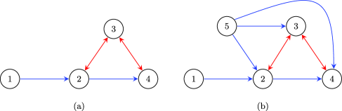
Figure 1: (a) An acyclic directed mixed graph, $\mathcal{L}$. (b) An ADMG studied by Evans and Richardson (2013).

Like DAGs, acyclic directed mixed graphs can be interpreted, via a Markov property, as representing a set of probability distributions defined by conditional independence restrictions; these can be read off the graph using a graphical separation criterion. The advantage of ADMGs is that they are closed under marginalization, in the sense mentioned above [Richardson and Spirtes (2002)]; indeed they represent precisely the conditional independence relations which can be obtained by marginalizing DAGs. Richardson (2003) gave a global Markov property and ordered local Markov property for ADMG models, and showed their equivalence.

The patterns of conditional independence implied by a DAG give rise to curved exponential families in the case of discrete random variables and, therefore, these models have well understood asymptotic statistical properties. However, general models induced by conditional independence constraints do not share this property, and it may be challenging to determine their dimension; for example, certain interpretations of chain graphs are known to lead to non-smooth models [Drton (2009)]. In this paper, we show that discrete ADMG models are curved exponential families, and give a smooth parameterization.

Evans and Richardson (2013) provide a number of applied examples for ADMGs representing discrete distributions—such as using the graph in Figure 1(b) to model an encouragement design for an influenza vaccine—and they discuss the relationship between Markovian ADMG models and marginal log-linear models [Bergsma and Rudas (2002), Bartolucci, Colombi and Forcina (2007)]. ADMGs also arise in studying general conditions for identifying intervention distributions, under the causal interpretation of a DAG model [see Dawid and Didelez (2010), Huang and Valtorta (2006), Pearl and Robins (1995), Shpitser and Pearl (2006a, 2006b), Tian and Pearl (2002), Silva and Ghahramani (2009)].

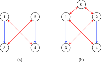
Figure 2: (a) An ADMG in which there is no vertex ordering such that all parents of a head precede every vertex in the head; (b) $\{0,3,4\}$ forms a head in this ADMG, but the induced subgraph on $\{0,3,4\}$ is not connected.

This paper provides a factorization criterion for joint distributions obeying the global Markov property with respect to an ADMG as well as a parameterization of these models in the discrete case. The factorizations so obtained are unusual: the graph in Figure 2(a), for example, gives

$$f_{1234}(x_{1},x_{2},x_{3},x_{4}) = f_{23|1}(x_{2},x_{3}\mid x_{1})\cdot f_{14|2}(x_{1},x_{4}\mid x_{2}),$$

showing that the joint distribution is a product of two conditional distributions that we would not usually expect to multiply together (see Example 4.13). The factorization criterion generalizes the well known one for DAGs, and is analogous to the Hammersley–Clifford theorem for undirected graphical models [Hammersley and Clifford (1971)]; the parameterization enables model fitting, and is used to prove that the discrete models are curved exponential families of distributions.

ADMGs may be viewed as a subclass of the larger classes of summary graphs [Wermuth (2011)] and ribbonless mixed graphs [Sadeghi (2013), Sadeghi and Lauritzen (2014)], which allow for undirected edges. The factorization and parameterization developed here may be extended to these larger classes without difficulty.

The remainder of the paper is organized as follows: Section 2 introduces basic graphical concepts. In Section 3, we give conditions under which a partial ordering on a class of subsets may be used to define partitions of arbitrary subsets. In Section 4, we use these tools to develop our factorization criterion, which then forms the basis of the simple parameterization introduced in Section 5. In Section 6, we show that the Markov model associated with an ADMG is smooth, and characterize the variation dependence of the parameterization. Finally, Section 7 contains a brief discussion.

2 Graphical definitions and Markov properties

Let $\mathcal{G}$ be an acyclic directed mixed graph with vertices $V$; the induced subgraph of $\mathcal{G}$ over $A\subseteq V$, denoted $\mathcal{G}_{A}$, is the graph with vertex set $A$, and all those (directed or bidirected) edges which join two vertices that are both in $A$.

A path in $\mathcal{G}$ is a sequence of adjacent edges, without repetition of a vertex; a path may be empty, or equivalently consist of only one vertex. The first and last vertices on a path are the endpoints (these are not distinct if the path is empty); other vertices on the path (if any) are non-endpoints. The graph $\mathcal{L}$ in Figure 1(a), for example, contains the path $1\rightarrow 2\rightarrow 4\leftrightarrow 3$, with endpoints 1 and 3, and non-endpoints 2 and 4. A directed path is one in which all the edges are directed ($\rightarrow$) and are oriented in the same direction, whereas a bidirected path consists entirely of bidirected edges.

We use the usual familial terminology for vertices in a graph. If $w\rightarrow v$, we say that $w$ is a parent of $v$; the set of parents of $v$ is denoted $\operatorname{pa}_{\mathcal{G}}(v)$. More generally, $w$ is an ancestor of $v$ if there is a directed path from $w$ to $v$ (note that this includes the case $v=w$); conversely $v$ is a descendant of $w$. The ancestors and descendants of $v$ are denoted $\operatorname{an}_{\mathcal{G}}(v)$ and $\operatorname{de}_{\mathcal{G}}(v)$, respectively. In the graph $\mathcal{L}$ in Figure 1(a), for instance, the ancestors of 4 are the vertices $\operatorname{an}_{\mathcal{L}}(4)=\{1,2,4\}$, and

$$\operatorname{pa}_{\mathcal{L}}(4)=\{2\},\qquad\operatorname{de}_{\mathcal{L}}(4)=\{4\}.$$

The district containing $v$, denoted $\operatorname{dis}_{\mathcal{G}}(v)$, is the set of vertices $w$ such that $v\leftrightarrow\cdots\leftrightarrow w$, including $v$ itself; for example, the district of 4 in $\mathcal{L}$ is $\{2,3,4\}$. We apply these functions disjunctively to sets so that, for example,

$$\operatorname{an}_{\mathcal{G}}(W)=\bigcup_{v\in W}\operatorname{an}_{\mathcal{G}}(v).$$

A set of vertices $A$ is ancestral if $A=\operatorname{an}_{\mathcal{G}}(A)$; that is, $A$ contains all its own ancestors. Define

$$\operatorname{barren}_{\mathcal{G}}(B)\equiv\bigl{\{}v\in B|\operatorname{de}_{\mathcal{G}}(v)\cap B=\{v\}\bigr{\}}.$$

We say a set $B$ is barren if $B=\operatorname{barren}_{\mathcal{G}}(B)$; that is, it contains none of its nontrivial descendants in $\mathcal{G}$. We will also use the notation $\operatorname{dis}_{A}(v)$ as a shorthand for $\operatorname{dis}_{\mathcal{G}_{A}}(v)$, the district containing $v$ in the induced subgraph of $\mathcal{G}$ on $A$.

For an ADMG $\mathcal{G}$ with vertex set $V$, we consider collections of random variables $(X_{v})_{v\in V}$ taking values in probability spaces $({\mathfrak{X}}_{v})_{v\in V}$; these spaces are either finite discrete sets or finite-dimensional real vector spaces. For $A\subseteq V$, we let ${\mathfrak{X}}_{A}\equiv\mbox{{$\times$}}_{v\in A}({\mathfrak{X}}_{v})$, ${\mathfrak{X}}\equiv{\mathfrak{X}}_{V}$ and $X_{A}\equiv(X_{v})_{v\in A}$. We abuse notation in the usual way: $v$ denotes both a vertex and the random variable $X_{v}$, likewise $A$ denotes both a set of vertices and the random vector $X_{A}$. For fixed elements of $\mathfrak{X}_{v}$ and $\mathfrak{X}_{A}$, we write $x_{v}$ and $x_{A}$, respectively.

The relationship between a graph $\mathcal{G}$ and random variables $X_{V}$ is governed by Markov properties specified in terms of paths. A non-endpoint vertex $c$ on a path $\pi$, is a collider on $\pi$ if the edges preceding and succeeding $c$ on the path both have an arrowhead at $c$, for example, $\rightarrow c\leftarrow$ or $\leftrightarrow c\leftarrow$; otherwise $c$ is a non-collider.

Definition 2.1.

A path $\pi$ in $\mathcal{G}$ between two vertices $v,w\in V(\mathcal{G})$ is said to be blocked by a set $C\subseteq V\setminus\{v,w\}$ if either: [(ii)]

there is a non-collider on $\pi$, and that non-collider is contained in $C$; or

there is a collider on $\pi$ which is not in $\operatorname{an}_{\mathcal{G}}(C)$. We say $v$ and $w$ are m-separated given $C$ in $\mathcal{G}$ if every path from $v$ to $w$ in $\mathcal{G}$ is blocked by $C$. Note that $C$ may be empty. Sets $A,B\subseteq V$ are said to be m-separated given $C\subseteq V\setminus(A\cup B)$ if every pair $a\in A$ and $b\in B$ are m-separated given $C$.

The special case of m-separation for DAGs is the better known d-separation [Pearl (1988), Lauritzen (1996)]. We next relate m-separation to conditional independence, for which we use the now standard notation of Dawid (1979): for random variables $X$, $Y$ and $Z$ we denote the statement “$X$ is independent of $Y$ conditional on $Z$” by $X\mathchoice{\mathrel{\hbox to0.0pt{$\displaystyle\perp$\hss}\mkern 2.0mu{\displaystyle\perp}}}{\mathrel{\hbox to0.0pt{$\textstyle\perp$\hss}\mkern 2.0mu{\textstyle\perp}}}{\mathrel{\hbox to0.0pt{$\scriptstyle\perp$\hss}\mkern 2.0mu{\scriptstyle\perp}}}{\mathrel{\hbox to0.0pt{$\scriptscriptstyle\perp$\hss}\mkern 2.0mu{\scriptscriptstyle\perp}}}Y|Z$. If $Z$ is empty, we write $X\mathchoice{\mathrel{\hbox to0.0pt{$\displaystyle\perp$\hss}\mkern 2.0mu{\displaystyle\perp}}}{\mathrel{\hbox to0.0pt{$\textstyle\perp$\hss}\mkern 2.0mu{\textstyle\perp}}}{\mathrel{\hbox to0.0pt{$\scriptstyle\perp$\hss}\mkern 2.0mu{\scriptstyle\perp}}}{\mathrel{\hbox to0.0pt{$\scriptscriptstyle\perp$\hss}\mkern 2.0mu{\scriptscriptstyle\perp}}}Y$.

Definition 2.2.

A probability measure $P$ on $\mathfrak{X}$ is said to satisfy the global Markov property (GMP) for an acyclic directed mixed graph $\mathcal{G}$, if for all disjoint sets $A,B,C\subseteq V$ with $A$ and $B$ nonempty, $A$ being m-separated from $B$ given $C$ implies that $X_{A}\mathchoice{\mathrel{\hbox to0.0pt{$\displaystyle\perp$\hss}\mkern 2.0mu{\displaystyle\perp}}}{\mathrel{\hbox to0.0pt{$\textstyle\perp$\hss}\mkern 2.0mu{\textstyle\perp}}}{\mathrel{\hbox to0.0pt{$\scriptstyle\perp$\hss}\mkern 2.0mu{\scriptstyle\perp}}}{\mathrel{\hbox to0.0pt{$\scriptscriptstyle\perp$\hss}\mkern 2.0mu{\scriptscriptstyle\perp}}}X_{B}|X_{C}$ under $P$.

Consider the ADMG $\mathcal{L}$ in Figure 1(a); the vertices 1 and 4 are m-separated conditional on 2, and 1 and 3 are m-separated unconditionally. It is not hard to verify that no other m-separation relations hold for this graph, and that therefore a distribution $P$ obeys the global Markov property with respect to $\mathcal{G}$ if and only if $X_{1}\mathchoice{\mathrel{\hbox to0.0pt{$\displaystyle\perp$\hss}\mkern 2.0mu{\displaystyle\perp}}}{\mathrel{\hbox to0.0pt{$\textstyle\perp$\hss}\mkern 2.0mu{\textstyle\perp}}}{\mathrel{\hbox to0.0pt{$\scriptstyle\perp$\hss}\mkern 2.0mu{\scriptstyle\perp}}}{\mathrel{\hbox to0.0pt{$\scriptscriptstyle\perp$\hss}\mkern 2.0mu{\scriptscriptstyle\perp}}}X_{4}|X_{2}$ and $X_{1}\mathchoice{\mathrel{\hbox to0.0pt{$\displaystyle\perp$\hss}\mkern 2.0mu{\displaystyle\perp}}}{\mathrel{\hbox to0.0pt{$\textstyle\perp$\hss}\mkern 2.0mu{\textstyle\perp}}}{\mathrel{\hbox to0.0pt{$\scriptstyle\perp$\hss}\mkern 2.0mu{\scriptstyle\perp}}}{\mathrel{\hbox to0.0pt{$\scriptscriptstyle\perp$\hss}\mkern 2.0mu{\scriptscriptstyle\perp}}}X_{3}$ under $P$.

Definition 2.3.

Let $\mathcal{G}$ be an ADMG containing an ancestral set $A$ and a vertex $v\in\operatorname{barren}_{\mathcal{G}}(A)$. Define

$$\operatorname{mb}_{\mathcal{G}}(v,A)\equiv\operatorname{pa}_{\mathcal{G}}\bigl{(}\operatorname{dis}_{A}(v)\bigr{)}\cup\bigl{(}\operatorname{dis}_{A}(v)\setminus\{v\}\bigr{)}$$

to be the Markov blanket for $v$ in the induced subgraph $\mathcal{G}_{A}$. For a set of vertices $W\subseteq\operatorname{barren}_{\mathcal{G}}(A)$, we analogously define the Markov blanket of $W$ to be

$$\operatorname{mb}_{\mathcal{G}}(W,A)\equiv\operatorname{pa}_{\mathcal{G}}\bigl{(}\operatorname{dis}_{A}(W)\bigr{)}\cup\bigl{(}\operatorname{dis}_{A}(W)\setminus W\bigr{)}.$$

Let $<$ be a topological ordering on the vertices of $\mathcal{G}$, meaning that no vertex appears before any of its ancestors; let ${\rm Phys.~{}Rev.~{}E}_{\mathcal{G},<}(v)$ be the set of vertices containing $v$ and all vertices preceding $v$ in the ordering. A probability measure $P$ is said to satisfy the ordered local Markov property for $\mathcal{G}$ with respect to $<$, if for any $v$ and ancestral set $A$ such that $v\in A\subseteq{\rm Phys.~{}Rev.~{}E}_{\mathcal{G},<}(v)$,

$$v\mathchoice{\mathrel{\hbox to0.0pt{$\displaystyle\perp$\hss}\mkern 2.0mu{\displaystyle\perp}}}{\mathrel{\hbox to0.0pt{$\textstyle\perp$\hss}\mkern 2.0mu{\textstyle\perp}}}{\mathrel{\hbox to0.0pt{$\scriptstyle\perp$\hss}\mkern 2.0mu{\scriptstyle\perp}}}{\mathrel{\hbox to0.0pt{$\scriptscriptstyle\perp$\hss}\mkern 2.0mu{\scriptscriptstyle\perp}}}A\setminus\bigl{(}\operatorname{mb}_{\mathcal{G}}(v,A)\cup\{v\}\bigr{)}|\operatorname{mb}_{\mathcal{G}}(v,A)$$

with respect to $P$.

Remark 2.4.

For $v\in\operatorname{barren}_{\mathcal{G}}(A)$, the Markov blanket for $v$ in $A$ consists of those vertices in $A\setminus\{v\}$ that can be reached from $v$ by paths through $A$ on which all non-endpoints are colliders.

Example 2.5.

One can easily verify that for the graph in Figure 1(a),

$$\operatorname{mb}_{\mathcal{L}}\bigl{(}4,\{1,2,4\}\bigr{)}=\{2\},\qquad\operatorname{mb}_{\mathcal{L}}\bigl{(}3,\{1,3\}\bigr{)}=\varnothing,$$

and that therefore under the topological ordering $1,2,3,4$, the ordered local Markov property implies $X_{4}\mathchoice{\mathrel{\hbox to0.0pt{$\displaystyle\perp$\hss}\mkern 2.0mu{\displaystyle\perp}}}{\mathrel{\hbox to0.0pt{$\textstyle\perp$\hss}\mkern 2.0mu{\textstyle\perp}}}{\mathrel{\hbox to0.0pt{$\scriptstyle\perp$\hss}\mkern 2.0mu{\scriptstyle\perp}}}{\mathrel{\hbox to0.0pt{$\scriptscriptstyle\perp$\hss}\mkern 2.0mu{\scriptscriptstyle\perp}}}X_{1}|X_{2}$ and $X_{3}\mathchoice{\mathrel{\hbox to0.0pt{$\displaystyle\perp$\hss}\mkern 2.0mu{\displaystyle\perp}}}{\mathrel{\hbox to0.0pt{$\textstyle\perp$\hss}\mkern 2.0mu{\textstyle\perp}}}{\mathrel{\hbox to0.0pt{$\scriptstyle\perp$\hss}\mkern 2.0mu{\scriptstyle\perp}}}{\mathrel{\hbox to0.0pt{$\scriptscriptstyle\perp$\hss}\mkern 2.0mu{\scriptscriptstyle\perp}}}X_{1}$, just as the global Markov property does.

The following result shows that the two properties are, in fact, always equivalent.

Proposition 2.6 ([Richardson (2003), Theorem 2])

Let $\mathcal{G}$ be an ADMG, and $<$ a topological ordering of its vertices; further let $P$ be a probability measure on $\mathfrak{X}_{V}$. The following are equivalent: [(ii)]

$P$ obeys the global Markov property with respect to $\mathcal{G}$;

$P$ obeys the ordered local Markov property with respect to $\mathcal{G}$ and $<$.

In particular, this result implies that if the ordered local Markov property is satisfied for some topological ordering $<$, then it is satisfied for all such orderings.

3 Partitions and partial orderings

The global Markov property for DAGs can be equivalently stated in terms of a simple factorization criterion applied to the joint distribution. In order to achieve something similar for ADMGs, we will need to consider partitions of sets of vertices into appropriate blocks. This section develops the necessary mathematical theory on functions that define partitions.

Let $V$ be an arbitrary finite set, and let $\mathcal{H}$ be a collection of nonempty subsets of $V$, with the restriction that $\{v\}\in\mathcal{H}$ for all $v\in V$ (i.e., all singletons are in $\mathcal{H}$). Let $\prec$ be a partial ordering on the elements of $\mathcal{H}$, and write $H_{1}\preceq H_{2}$ to mean that either $H_{1}\prec H_{2}$ or $H_{1}=H_{2}$.

Definition 3.1.

We say that $\prec$ is partition-suitable (for $\mathcal{H}$) if for any $H_{1},H_{2}\in\mathcal{H}$ with $H_{1}\cap H_{2}\neq\varnothing$, there exists $H^{*}\in\mathcal{H}$ such that $H^{*}\subseteq H_{1}\cup H_{2}$ and $H_{i}\preceq H^{*}$ for each $i=1,2$.

In other words, partition-suitability requires that any two intersecting elements of $\mathcal{H}$ are dominated with respect to $\prec$ by some element of $\mathcal{H}$.

Define a function $\Phi$ on subsets of $V$ such that $\Phi(W)$ “picks out” the $\prec$-maximal elements of $\mathcal{H}$ which are subsets of $W$. That is, it returns the collection of subsets

$$\Phi(W)\equiv\bigl{\{}H\in\mathcal{H}|H\subseteq W\mbox{ and }H\nprec H^{\prime}\mbox{ for all other }H^{\prime}\subseteq W\bigr{\}}.$$

Partition-suitability ensures that the sets in $\Phi(W)$ are disjoint.

Proposition 3.2

If $\prec$ is partition-suitable and $H_{1},H_{2}\in\Phi(A)$ for some set $A$, then either $H_{1}=H_{2}$ or $H_{1}\cap H_{2}=\varnothing$.

This is immediate from the definition of partition-suitable.

Now let

$$\psi(W)\equiv W\setminus\bigcup_{C\in\Phi(W)}C,$$

that is, $\psi$ returns those elements of $W$ which are not contained in any set in $\Phi(W)$. Then recursively define a partitioning function $[\cdot]$ on subsets of $V$ by $[\varnothing]=\varnothing$, and

$$[W]\equiv\Phi(W)\cup\bigl{[}\psi(W)\bigr{]}.$$

The idea is that the function $\Phi$ “removes” the maximal sets from $W$, and the procedure is then applied again to what remains, $\psi(W)$. The following proposition shows that each vertex of $W$ is contained within precisely one set in $[W]$.

Proposition 3.3

If $\prec$ is partition-suitable, then the function $[\cdot]$ partitions sets. That is, for any $W\subseteq V$,

$$\bigcup_{H\in[W]}H=W,$$

and if $A,B\in[W]$ then either $A=B$ or $A\cap B=\varnothing$.

We proceed by induction on the size of $W$. If $W=\varnothing$ the result follows from the definition. Also by definition, if $W\neq\varnothing$ then

$$[W]=\Phi(W)\cup\bigl{[}\psi(W)\bigr{]},$$

so the induction hypothesis and the definitions of $\Phi$ and $\psi$ mean we need only check that $\Phi(W)$ is nonempty and contains disjoint sets.

The first claim follows from the fact that $\prec$ is a partial ordering, and so always contains at least one maximal element (since $V$ is finite); the second is a direct application of Proposition 3.2.

Lemma 3.4

Let $\prec$ be partition-suitable, $A\subseteq V$ and $H\in\Phi(A)$. If $H\subseteq B\subseteq A$ for some subset $B$, then $H\in\Phi(B)$.

Let $\mathcal{H}_{A}$ be the set of subsets in $\mathcal{H}$ contained within $A$. If $H\in\Phi(A)\subseteq\mathcal{H}_{A}$ then $H$ is maximal with respect to $\prec$ in $\mathcal{H}_{A}$. It is trivial that $\mathcal{H}_{B}\subseteq\mathcal{H}_{A}$, and so $H$ is also maximal in $\mathcal{H}_{B}$. Thus, $H\in\Phi(B)$.

We can paraphrase Lemma 3.4 as saying that if a set $H$ is removed from $A$ at the first application of $\Phi$, then $H$ is contained in the partition of any subset $B$ of $A$ (provided $B$ contains $H$).

The next proposition shows that partitioning functions as we have defined them are stable when some set in the partition is removed. This “stability” is very useful when trying to understand the properties of the partition.

Proposition 3.5

If $C\in[W]$, then $[W]=\{C\}\cup[W\setminus C]$.

We proceed by induction on the size of $W$. If $[W]=\{C\}$, including any case in which $|W|=1$, the result is trivial.

If $C$ is not maximal with respect to $\prec$ in $W$ then, by Lemma 3.4, $\Phi(W)=\Phi(W\setminus C)$, so

$$[W] = \Phi(W)\cup\bigl{[}\psi(W)\bigr{]}$$

$$= \Phi(W\setminus C)\cup\bigl{[}\psi(W)\bigr{]},$$

and the problem reduces to showing that

$$\bigl{[}\psi(W)\bigr{]}=\{C\}\cup\bigl{[}\psi(W\setminus C)\bigr{]}=\{C\}\cup\bigl{[}\psi(W)\setminus C\bigr{]},$$

which holds by the induction hypothesis. Thus, without loss of generality, suppose $C\in\Phi(W)$.

Now, by Lemma 3.4 and the supposition, $\Phi(W\setminus C)\cup\{C\}\supseteq\Phi(W)$, and if equality holds we are done. Otherwise let $C_{1},\ldots,C_{k}$ be the sets in $\Phi(W\setminus C)$ but not in $\Phi(W)$. Note that by definition, $C_{1},\ldots,C_{k}\subseteq\psi(W)$. Further, these sets are maximal in $W\setminus C$, so by Lemma 3.4 they are also maximal in $\psi(W)\subseteq W\setminus C$. Then the problem reduces to showing that

$$\bigl{[}\psi(W)\bigr{]}=\{C_{1},\ldots,C_{k}\}\cup\bigl{[}\psi(W)\setminus(C_{1}\cup\cdots\cup C_{k})\bigr{]},$$

which follows from repeated application of the induction hypothesis.

Lastly, we show that if each set in $\mathcal{H}$ is contained within a piece of some partition of $V$, then the partitioning function can be applied separately to each piece of this coarser partition.

Proposition 3.6

Let $D_{1},\ldots,D_{k}$ be a partition of $V$, and suppose that every $H\in\mathcal{H}$ is contained within some $D_{i}$. Let $\prec$ be a partition-suitable partial ordering on $\mathcal{H}$. Then for all $W\subseteq V$,

$$[W]=\bigcup_{i=1}^{k}[W\cap D_{i}].$$

We prove the case $k=2$, from which the general result follows by repeated applications. If either of $W\cap D_{1}$ or $W\cap D_{2}$ are empty, then the result is trivial. By definitions

$$[W]=\Phi(W)\cup\bigl{[}\psi(W)\bigr{]};$$

$\psi(W)$ is strictly smaller than $W$, so by the induction hypothesis

$$[W]=\Phi(W)\cup\bigl{[}\psi(W)\cap D_{1}\bigr{]}\cup\bigl{[}\psi(W)\cap D_{2}\bigr{]}.$$

Define $\mathcal{C}_{1}$, $\mathcal{C}_{2}$ so that $\Phi(W)=\mathcal{C}_{1}\cup\mathcal{C}_{2}$ and each $H\in\mathcal{C}_{i}$ is a subset of $D_{i}$ only; since the elements of $\mathcal{C}_{i}$ are maximal with respect to $\prec$ in $W$, by Lemma 3.4 they are also maximal in $W\cap D_{i}$. Hence, $\mathcal{C}_{i}\subseteq\Phi(W\cap D_{i})$. Repeatedly applying Proposition 3.5 gives

$$\mathcal{C}_{i}\cup\bigl{[}\psi(W)\cap D_{i}\bigr{]} = [W\cap D_{i}],$$

because $(\psi(W)\cap D_{i})\cup\bigcup_{C\in\mathcal{C}_{i}}C=W\cap D_{i}$. Hence the result.

4 The factorization criterion

Let $P$ be a probability measure having density $f_{V}\dvtx\mathfrak{X}_{V}\rightarrow\mathbb{R}$ with respect to some $\sigma$-finite dominating product measure $\mu$ on $\mathfrak{X}_{V}$. For $U,W\subseteq V$, we denote by $f_{W}\dvtx\mathfrak{X}_{W}\rightarrow\mathbb{R}$ the marginal density over $W$, and by $f_{W|U}(\cdot|u)\dvtx\mathfrak{X}_{W}\rightarrow\mathbb{R}$ for $f_{U}(u)>0$ the conditional density of $W$ given $U=u$ (more precisely: any member of the equivalence class of such densities). Then $P$ obeys the global Markov property with respect to a DAG if and only if it factorizes as

$$f_{V}(x_{V})=\prod_{v\in V}f_{v|\operatorname{pa}(v)}(x_{v}|x_{\operatorname{pa}(v)}),$$

for $\mu$-almost all $x_{V}\in\mathfrak{X}_{V}$ [see, e.g., Lauritzen (1996)]. In the sequel, all equalities over $f$ are considered to hold almost everywhere with respect to $\mu$.

In this section, we show that factorizations can also be used to characterize Markov models over ADMGs; however, as we shall see, the criterion is more complicated than that for DAGs.

Example 4.1.

Consider the ADMG in Figure 1(a). A distribution which obeys the global Markov property with respect to this graph satisfies $X_{1}\mathchoice{\mathrel{\hbox to0.0pt{$\displaystyle\perp$\hss}\mkern 2.0mu{\displaystyle\perp}}}{\mathrel{\hbox to0.0pt{$\textstyle\perp$\hss}\mkern 2.0mu{\textstyle\perp}}}{\mathrel{\hbox to0.0pt{$\scriptstyle\perp$\hss}\mkern 2.0mu{\scriptstyle\perp}}}{\mathrel{\hbox to0.0pt{$\scriptscriptstyle\perp$\hss}\mkern 2.0mu{\scriptscriptstyle\perp}}}X_{3}$ and $X_{1}\mathchoice{\mathrel{\hbox to0.0pt{$\displaystyle\perp$\hss}\mkern 2.0mu{\displaystyle\perp}}}{\mathrel{\hbox to0.0pt{$\textstyle\perp$\hss}\mkern 2.0mu{\textstyle\perp}}}{\mathrel{\hbox to0.0pt{$\scriptstyle\perp$\hss}\mkern 2.0mu{\scriptstyle\perp}}}{\mathrel{\hbox to0.0pt{$\scriptscriptstyle\perp$\hss}\mkern 2.0mu{\scriptscriptstyle\perp}}}X_{4}|X_{2}$. It is not possible to specify a factorization on the joint distribution of $X_{1}$, $X_{2}$, $X_{3}$ and $X_{4}$ which implies precisely these two independences. Instead, we require factorizations of certain marginal distributions:

$$f_{13}(x_{1},x_{3}) = f_{1}(x_{1})\cdot f_{3}(x_{3}),$$

$$f_{124}(x_{1},x_{2},x_{4}) = f_{1}(x_{1})\cdot f_{2|1}(x_{2}|x_{1})\cdot f_{4|2}(x_{4}|x_{2}).$$

Such marginal factorizations can be used to represent distributions which obey the global Markov property with respect to an ADMG.

Definition 4.2 ((Head)).

A vertex set $H\subseteq V$ is a head if it is barren in $\mathcal{G}$ and contained within a single district of $\mathcal{G}_{\operatorname{an}(H)}$. We write $\mathcal{H}(\mathcal{G})$ for the collection of all heads in $\mathcal{G}$.

Note that every singleton vertex $\{v\}$ forms a head.

Example 4.3.

For the ADMG shown in Figure 2(b), we have the following:

$$\mathcal{H}(\mathcal{G}) = \bigl{\{}\{0\},\{1\},\{2\},\{3\},\{4\},\{0,1\},\{0,2\},\{1,4\},\{2,3\},$$

$$\hskip 59.0pt\{0,1,2\},\{0,1,4\},\{0,2,3\},\{0,3,4\}\bigr{\}}.$$

Notice that although they are contained within a single district, the sets $\{0,1,2,4\}$, $\{0,1,2,3\}$ and $\{0,1,2,3,4\}$ do not form heads because they are not barren. Also observe that $\{0,3,4\}$ does form a head, even though the induced subgraph $\mathcal{G}_{\{0,3,4\}}$ is not connected [because $\{0,3,4\}$ is a subset of a single district in $\mathcal{G}_{\operatorname{an}(\{0,3,4\})}$, as required].

Definition 4.4 ((Tail)).

For any head $H$, the tail of $H$ is the set

$$\operatorname{tail}_{\mathcal{G}}(H)\equiv\bigl{(}\operatorname{dis}_{\operatorname{an}(H)}(H)\setminus H\bigr{)}\cup\operatorname{pa}\bigl{(}\operatorname{dis}_{\operatorname{an}(H)}(H)\bigr{)}.$$

If the context makes it clear which head we are referring to, we will sometimes denote a tail simply by $T$.

Note that the tail is a subset of the ancestors of the head. An intuitive interpretation is that a head $H$ is a set within which no independence relations hold without marginalizing some elements of $H$, and the tail is the Markov blanket for $H$ within the set $\operatorname{an}_{\mathcal{G}}(H)$. We can therefore factorize ancestral sets into heads conditional upon their tail sets; see Remark 4.14 below.

Example 4.5.

In the special case of a DAG, the heads are precisely all singleton vertices $\{v\}$, and the tails are the sets of parents $\operatorname{pa}_{\mathcal{G}}(v)$. In a purely bidirected graph, the heads are just the connected sets, and the tails are all empty.

Example 4.6.

The graph $\mathcal{L}$ in Figure 1(a) has the following head–tail pairs:

$H$	$\{1\}$	$\{2\}$	$\{3\}$	$\{2,3\}$	$\{4\}$	$\{3,4\}$
$T$	$\varnothing$	$\{1\}$	$\varnothing$	$\{1\}$	$\{2\}$	$\{1,2\}$

Note that the set $\{2,3,4\}$ is not a head, because it is not barren.

In general, it is not possible to order the vertices in an acyclic directed mixed graph such that, for each head $H$, all the vertices in $\operatorname{pa}_{\mathcal{G}}(H)$ precede all the vertices in $H$. A counterexample is given in Figure 2(a), which is taken from Richardson (2009). The head $\{1,4\}$ has parent 2, and the head $\{2,3\}$ has parent 1, so whichever way we order the vertices 1 and 2, the condition will be violated.

However, there is a well-defined partial ordering on heads which will be useful to us, and satisfies the essential property of partition-suitability from Section 3.

Definition 4.7.

For two distinct heads $H_{i}$ and $H_{j}$ in an ADMG $\mathcal{G}$, say that $H_{i}\prec H_{j}$ if $H_{i}\subseteq\operatorname{an}_{\mathcal{G}}(H_{j})$.

Lemma 4.8

The (strict) partial ordering $\prec$ is well defined.

We need to verify that $\prec$ is irreflexive, asymmetric and transitive; irreflexivity is by definition. Asymmetry amounts to $H_{i}\prec H_{j}\Longrightarrow H_{j}\nprec H_{i}$; suppose not for contradiction, so that there exist distinct heads $H_{i}$ and $H_{j}$ with $H_{i}\prec H_{j}$ and $H_{j}\prec H_{i}$. Since $H_{i}$ and $H_{j}$ are distinct, there exists a vertex $v$ which is in one of these heads but not the other; assume without loss of generality that $v\in H_{j}\setminus H_{i}$.

Since $H_{j}\subseteq\operatorname{an}_{\mathcal{G}}(H_{i})$, we can find a directed path $\pi_{1}$ from $v$ to some vertex $w\in H_{i}$; the path is nonempty because $v\notin H_{i}$. However, since we also have $H_{i}\subseteq\operatorname{an}_{\mathcal{G}}(H_{j})$, we can find a (possibly empty) directed path $\pi_{2}$ from $w$ to some $x\in H_{j}$. Now, the concatenation of $\pi_{1}$ and $\pi_{2}$ is also a path, because any repeated vertices would imply a directed cycle in the graph. Call this new path $\pi$.

But $\pi$ is a nonempty directed path between two vertices in $H_{j}$, which violates the requirement that heads are barren. Hence, asymmetry holds.

For transitivity, if $H_{i}\prec H_{j}$ and $H_{j}\prec H_{k}$, then clearly we can find a directed path from any element $v\in H_{i}$ to some element of $H_{k}$, simply by concatenating paths from $v\in H_{i}$ to some $w\in H_{j}$ and from $w$ to $H_{k}$. Hence, $H_{i}\subseteq\operatorname{an}_{\mathcal{G}}(H_{k})$, and so $H_{i}\prec H_{k}$.

Lemma 4.9

The partial ordering $\prec$ on the heads $\mathcal{H}(\mathcal{G})$ of an ADMG $\mathcal{G}$ is partition-suitable.

Proof sketch (see the Appendix for details) If two heads $H_{1},H_{2}$ are distinct and $H_{1}\cap H_{2}\neq\varnothing$, then $H^{*}=\operatorname{barren}_{\mathcal{G}}(H_{1}\cup H_{2})$ is a head, $H_{1}\preceq H^{*}$ and $H_{2}\preceq H^{*}$.

Note that in general $H^{*}$ may be a strict subset of $H_{1}\cup H_{2}$. For example, consider the graph shown in Figure 2(b), and let $H_{1}=\{0,1,4\}$ and $H_{2}=\{0,2,3\}$ so that $H_{1},H_{2}\in{\mathcal{H}}(\mathcal{G})$ and $H_{1}\cap H_{2}=\{0\}$. However, $H^{*}=\operatorname{barren}_{\mathcal{G}}(H_{1}\cup H_{2})=\{0,3,4\}\subsetneq H_{1}\cup H_{2}$.

Denote the relevant functions from Section 3 defined by this partial ordering by $\Phi_{\mathcal{G}}$, $\psi_{\mathcal{G}}$ and $[\cdot]_{\mathcal{G}}$, respectively. This partitioning function allows us to factorize probabilities for ADMGs into expressions based upon heads and tails.

Example 4.10.

For the graph $\mathcal{L}$ in Figure 1(a), we have

$H$	$\{1\}$	$\{2\}$	$\{3\}$	$\{2,3\}$	$\{4\}$	$\{3,4\}$
$\operatorname{an}_{\mathcal{G}}(H)$	$\{1\}$	$\{1,2\}$	$\{3\}$	$\{1,2,3\}$	$\{1,2,4\}$	$\{1,2,3,4\}$

so that

$$\{1\} \prec \{2\}\prec\{2,3\}\prec\{3,4\},$$

$$\{2\} \prec \{4\}\prec\{3,4\},\qquad\{3\}\prec\{2,3\}.$$

Then, for example, $\Phi_{\mathcal{L}}(\{2,3,4\})=\{\{3,4\}\}$, and $\Phi_{\mathcal{L}}(\{2\})=\{\{2\}\}$, giving

$$\bigl{[}\{2,3,4\}\bigr{]}_{\mathcal{L}}=\bigl{\{}\{3,4\},\{2\}\bigr{\}}.$$

Example 4.11.

For the graph in Figure 2(a), we have

$H$	$\{1\}$	$\{2\}$	$\{3\}$	$\{4\}$	$\{1,4\}$	$\{2,3\}$
$\operatorname{an}_{\mathcal{G}}(H)$	$\{1\}$	$\{2\}$	$\{1,3\}$	$\{2,4\}$	$\{1,2,4\}$	$\{1,2,3\}$

Thus $\{1\}\prec\{3\}\prec\{2,3\}\succ\{2\}$ and $\{2\}\prec\{4\}\prec\{1,4\}\succ\{1\}$.

Now we can provide a factorization criterion for acyclic directed mixed graphs.

Theorem 4.12

Let $\mathcal{G}$ be an ADMG, and $P$ a probability distribution on $\mathfrak{X}_{V}$ with density $f_{V}$. $P$ obeys the global Markov property with respect to $\mathcal{G}$ if and only if for every ancestral set $A\in\mathcal{A}(\mathcal{G})$, and $\mu$-almost all $x_{A}\in\mathfrak{X}_{A}$.

$$f_{A}(x_{A}) = \prod_{H\in[A]_{\mathcal{G}}}f_{H|T}(x_{H}|x_{T}).$$ (1)

A formal proof of this result is given in the Appendix; a sketch proof is given in Richardson (2009), Theorem 4.

Example 4.13.

For the graph in Figure 2(a), observe that the global Markov property implies precisely that $X_{3}\mathchoice{\mathrel{\hbox to0.0pt{$\displaystyle\perp$\hss}\mkern 2.0mu{\displaystyle\perp}}}{\mathrel{\hbox to0.0pt{$\textstyle\perp$\hss}\mkern 2.0mu{\textstyle\perp}}}{\mathrel{\hbox to0.0pt{$\scriptstyle\perp$\hss}\mkern 2.0mu{\scriptstyle\perp}}}{\mathrel{\hbox to0.0pt{$\scriptscriptstyle\perp$\hss}\mkern 2.0mu{\scriptscriptstyle\perp}}}X_{4}|X_{12}$, and $X_{1}\mathchoice{\mathrel{\hbox to0.0pt{$\displaystyle\perp$\hss}\mkern 2.0mu{\displaystyle\perp}}}{\mathrel{\hbox to0.0pt{$\textstyle\perp$\hss}\mkern 2.0mu{\textstyle\perp}}}{\mathrel{\hbox to0.0pt{$\scriptstyle\perp$\hss}\mkern 2.0mu{\scriptstyle\perp}}}{\mathrel{\hbox to0.0pt{$\scriptscriptstyle\perp$\hss}\mkern 2.0mu{\scriptscriptstyle\perp}}}X_{2}$. Applying the partition function to the relevant sets of vertices yields

$$\bigl{[}\{1,2,3,4\}\bigr{]} = \bigl{\{}\{1,4\},\{2,3\}\bigr{\}},$$

so Theorem 4.12 gives us the factorization from the Introduction:

$$f_{1234}(x_{1},x_{2},x_{3},x_{4}) = f_{23|1}(x_{2},x_{3}\mid x_{1})\cdot f_{14|2}(x_{1},x_{4}\mid x_{2})$$

for all $x_{i}\in\mathfrak{X}_{i}$, $i=1,\ldots,4$. The expression may appear slightly strange, since the first factor is the density for $\{X_{2},X_{3}\}$ given $X_{1}$, while the second is for $\{X_{1},X_{4}\}$ given $X_{2}$; nevertheless this factorization does indeed imply that $X_{3}\mathchoice{\mathrel{\hbox to0.0pt{$\displaystyle\perp$\hss}\mkern 2.0mu{\displaystyle\perp}}}{\mathrel{\hbox to0.0pt{$\textstyle\perp$\hss}\mkern 2.0mu{\textstyle\perp}}}{\mathrel{\hbox to0.0pt{$\scriptstyle\perp$\hss}\mkern 2.0mu{\scriptstyle\perp}}}{\mathrel{\hbox to0.0pt{$\scriptscriptstyle\perp$\hss}\mkern 2.0mu{\scriptscriptstyle\perp}}}X_{4}|X_{12}$. Further, integrating out $x_{3}$ and $x_{4}$ gives

$$f_{12}(x_{1},x_{2}) = f_{2|1}(x_{2}|x_{1})\cdot f_{1|2}(x_{1}|x_{2}),\qquad x_{1}\in\mathfrak{X}_{1},x_{2}\in\mathfrak{X}_{2},$$

which implies that $X_{1}\mathchoice{\mathrel{\hbox to0.0pt{$\displaystyle\perp$\hss}\mkern 2.0mu{\displaystyle\perp}}}{\mathrel{\hbox to0.0pt{$\textstyle\perp$\hss}\mkern 2.0mu{\textstyle\perp}}}{\mathrel{\hbox to0.0pt{$\scriptstyle\perp$\hss}\mkern 2.0mu{\scriptstyle\perp}}}{\mathrel{\hbox to0.0pt{$\scriptscriptstyle\perp$\hss}\mkern 2.0mu{\scriptscriptstyle\perp}}}X_{2}$.

Remark 4.14.

It follows from Theorem 4.12 that if $H$ is a head, $\operatorname{tail}_{\mathcal{G}}(H)$ is the Markov blanket for $H$ in the set $\operatorname{an}_{\mathcal{G}}(H)$, in the sense that under the global Markov property,

$$H\mathchoice{\mathrel{\hbox to0.0pt{$\displaystyle\perp$\hss}\mkern 2.0mu{\displaystyle\perp}}}{\mathrel{\hbox to0.0pt{$\textstyle\perp$\hss}\mkern 2.0mu{\textstyle\perp}}}{\mathrel{\hbox to0.0pt{$\scriptstyle\perp$\hss}\mkern 2.0mu{\scriptstyle\perp}}}{\mathrel{\hbox to0.0pt{$\scriptscriptstyle\perp$\hss}\mkern 2.0mu{\scriptscriptstyle\perp}}}\operatorname{an}_{\mathcal{G}}(H)\setminus\bigl{(}H\cup\operatorname{tail}_{\mathcal{G}}(H)\bigr{)}\mid\operatorname{tail}_{\mathcal{G}}(H).$$

Remark 4.15.

A different, incorrect definition of $\Phi_{\mathcal{G}}$ (and, therefore, $\psi_{\mathcal{G}}$, $[\cdot]_{\mathcal{G}}$) was given in Richardson (2009) and Evans and Richardson (2010). The erroneous definition coincides with that given here when $W$ is ancestral, so equation (1) holds for both. However, equation (2) below does not hold for the incorrect partitioning function in general.

5 Toward a parameterization of the discrete Markov model for an ADMG

The factorizations in Theorem 4.12 can be used to produce a parameterization of ADMG models when $\mathfrak{X}_{V}$ is a finite set, and thus the relevant random variables are discrete. For simplicity of exposition, we will henceforth assume that the random variables are binary, so $\mathfrak{X}_{V}=\{0,1\}^{|V|}$. Extension to the general finite discrete case is easy but notationally challenging; this is done in the special case of ADMGs with chain graph structure by Drton (2009).

In the following result, and throughout the paper, empty products are assumed to equal 1.

Theorem 5.1

Let $\mathcal{G}$ be an ADMG, and $P$ a probability distribution on $\{0,1\}^{|V|}$. Then $P$ obeys the global Markov property with respect to $\mathcal{G}$ if and only if for every ancestral set $A$ and $x_{A}\in\mathfrak{X}_{A}$,

$$P(X_{A}=x_{A}) = \sum_{C\dvtx O\subseteq C\subseteq A}(-1)^{|C\setminus O|}\prod_{H\in[C]_{\mathcal{G}}}P(X_{H}={0}|X_{T}=x_{T}),$$ (2)

where $O\equiv\{v\in A|x_{v}=0\}$.

Theorem 5.1 shows that conditional probabilities of the form $P(X_{H}=0|X_{T}=x_{T})$ are sufficient to form a parameterization of the binary ADMG model; it remains to show that they are nonredundant, which is proved in Section 6.

Note that the sets $C$ in (2) may not be ancestral, which hinders proof by induction. In order to facilitate the proof, we define the following quantity which will be needed in the intermediate steps of the induction.

Definition 5.2.

Let $A$ be an ancestral set in an ADMG $\mathcal{G}$, and consider a particular assignment $x_{A}$ to $X_{A}$; write $O\equiv\{v\in A|x_{v}=0\}$. For any sets $B$, $W$ such that $B\subseteq W\subseteq(A\setminus O)$, define the following quantity:

$$g_{x_{A}}(B,W) \equiv (-1)^{|B|}\prod_{H\in[O\cup W]_{\mathcal{G}}}P(X_{H\cap(O\cup B)}={0},X_{H\setminus(O\cup B)}={1}\mid X_{T}=x_{T}).$$

Note that if $B=\varnothing$ then the right-hand side has factors of the form $P(X_{H}=x_{H}|X_{T}=x_{T})$, and looks much like (1); however, if $B=W$ the expression is a product of the form $P(X_{H}=0|X_{T}=x_{T})$, just like each term of (2).

The interpretation is that $W$ is the set of nonzero vertices being partitioned, and which need to have their values on the left-hand side of any conditioning bars “flipped” from 1 to 0 in order to get an expression of the form (2). The set $B$ consists of those vertices for which this “flipping” has already taken place, and those in $W\setminus B$ have yet to be flipped.

The induction starts with the single term $(B,W)=(\varnothing,A\setminus O)$, given via Theorem 4.12. At each step a term is “reduced” into a sum of two further pieces by flipping a single vertex, until the procedure finishes with a sum containing the set of terms

$$\bigl{\{}g_{x_{A}}(B,W)\dvtx(B,W)=(C,C),\mbox{ where }C\subseteq A\setminus O\bigr{\}},$$

and thus corresponds to an expression of the form (2).

Definition 5.3.

Take a triple $(x_{A},B,W)$, where $B\subsetneq W\subseteq(A\setminus O)$ for $O\equiv\{v\in A|x_{v}=0\}$. We say that $(x_{A},B,W)$ is reducible if for each $H\in[O\cup W]_{\mathcal{G}}$ such that $H\cap(W\setminus B)\neq\varnothing$, it holds that $\operatorname{dis}_{\operatorname{an}(H)}(H)\setminus H\subseteq O\cup(W\setminus B)$.

In words, given a set $W$ in which not all vertices are flipped, so $W\setminus B\neq\varnothing$, the condition requires that any head $H$ which is in the partition and has not yet been fully “flipped,” has the part of its tail which is from the same district [i.e., $\operatorname{dis}_{\operatorname{an}(H)}(H)\setminus H$] consists solely of vertices that are either in $W$ or not yet flipped.

The following technical lemma provides the necessary piece for the induction step.

Lemma 5.4

Let $A$ be an ancestral set, and $P$ a distribution obeying the global Markov property with respect to $\mathcal{G}$. If $(x_{A},B,W)$ is reducible in $\mathcal{G}_{A}$, then there is some $w\in W\setminus B$ such that

$$g_{x_{A}}(B,W)=g_{x_{A}}\bigl{(}B,W\setminus\{w\}\bigr{)}+g_{x_{A}}\bigl{(}B\cup\{w\},W\bigr{)},$$ (3)

and, in addition, either $B=W\setminus\{w\}$ (so $B\cup\{w\}=W$), or both $(x_{A},B,W\setminus\{w\})$ and $(x_{A},B\cup\{w\},W)$ are also reducible.

See the Appendix.

Here, $w$ is a vertex that is given the value $1$ in every head in $g_{x_{V}}(B,W)$, but is “flipped” so it is set equal to $0$ in $g_{x_{V}}(B\cup\{w\},W)$ and is removed from the partition in $g_{x_{V}}(B,W\setminus\{w\})$. A major difficulty in the overall proof of Theorem 5.1 stems from the fact that, though each $g_{x_{A}}$ produced after a reduction is itself reducible or of the form $g_{x_{A}}(C,C)$, we will not generally be able to flip the same vertex in each term.

Proof of Theorem 5.1 By Theorem 4.12, the global Markov property holds if and only if for each ancestral $A$ and $x_{A}$,

$$P(X_{A}=x_{A}) = \prod_{H\in[A]_{\mathcal{G}}}P(X_{H}=x_{H}|X_{T}=x_{T})$$

$$= g_{x_{A}}(\varnothing,A\setminus O)$$

using the definition of $g_{x_{V}}$. It is easy to check from Definition 5.3 that either $A=O$, in which case there is nothing to prove, or $(x_{A},\varnothing,A\setminus O)$ is reducible. Then from repeated application of Lemma 5.4 this is just

$$= \sum_{C\subseteq A\setminus O}g_{x_{A}}(C,C)$$

$$= \sum_{C\subseteq A\setminus O}(-1)^{|C|}\prod_{H\in[O\cup C]_{\mathcal{G}}}P(X_{H}=0|X_{T}=x_{T})$$

which, by inspection, gives the required result. Conversely, suppose (2) holds, and that $v\in\operatorname{barren}_{\mathcal{G}}(A)$ has district $D_{1}=\operatorname{dis}_{A}(v)$; let $D_{2}\equiv A\setminus D_{1}$ and for $C\subseteq A$, let $C_{i}\equiv C\cap D_{i}$ and $O_{i}\equiv O\cap D_{i}$, $i=1,2$. Then $C\setminus O=(C_{1}\setminus O_{1})\,\dot{\cup}\,\break(C_{2}\setminus O_{2})$, and from Proposition 3.6 get $[C]_{\mathcal{G}}=[C_{1}]_{\mathcal{G}}\cup[C_{2}]_{\mathcal{G}}$. Hence,

$$P(X_{A}=x_{A}) = \sum_{C\dvtx O\subseteq C\subseteq A}(-1)^{|C\setminus O|}\prod_{H\in[C]_{\mathcal{G}}}P(X_{H}=0\mid X_{T}=x_{T})$$

$$= \mathop{\sum_{C_{1}\dvtx O_{1}\subseteq C_{1}\subseteq D_{1}}}_{C_{2}\dvtx O_{2}\subseteq C_{2}\subseteq D_{2}}(-1)^{\mid C_{1}\setminus O_{1}|+|C_{2}\setminus O_{2}|}$$

$${}\times\prod_{H\in[C_{1}]_{\mathcal{G}}\cup[C_{2}]_{\mathcal{G}}}P(X_{H}=0\mid X_{T}=x_{T})$$

$$= \sum_{C_{1}\dvtx O_{1}\subseteq C_{1}\subseteq D_{1}}(-1)^{\mid C_{1}\setminus O_{1}|}\prod_{H\in[C_{1}]_{\mathcal{G}}}P(X_{H}=0\mid X_{T}=x_{T})$$

$${}\times\sum_{C_{2}\dvtx O_{2}\subseteq C_{2}\subseteq D_{2}}(-1)^{|C_{2}\setminus O_{2}|}\prod_{H\in[C_{2}]_{\mathcal{G}}}P(X_{H}=0\mid X_{T}=x_{T})$$

$$= h(x_{D_{1}},x_{\operatorname{pa}_{\mathcal{G}}(D_{1})})\cdot k(x_{D_{2}},x_{\operatorname{pa}_{\mathcal{G}}(D_{2})})$$

for some functions $h,k$. In particular, $k$ does not involve $x_{v}$, so it follows that $v\mathchoice{\mathrel{\hbox to0.0pt{$\displaystyle\perp$\hss}\mkern 2.0mu{\displaystyle\perp}}}{\mathrel{\hbox to0.0pt{$\textstyle\perp$\hss}\mkern 2.0mu{\textstyle\perp}}}{\mathrel{\hbox to0.0pt{$\scriptstyle\perp$\hss}\mkern 2.0mu{\scriptstyle\perp}}}{\mathrel{\hbox to0.0pt{$\scriptscriptstyle\perp$\hss}\mkern 2.0mu{\scriptscriptstyle\perp}}}A\setminus(D_{1}\cup\operatorname{pa}_{\mathcal{G}}(D_{1}))\mid(D_{1}\setminus\{v\})\cup\operatorname{pa}_{\mathcal{G}}(D_{1})$ which, by the definition of the Markov blanket of $v$ in $A$, is equivalent to

$$v\mathchoice{\mathrel{\hbox to0.0pt{$\displaystyle\perp$\hss}\mkern 2.0mu{\displaystyle\perp}}}{\mathrel{\hbox to0.0pt{$\textstyle\perp$\hss}\mkern 2.0mu{\textstyle\perp}}}{\mathrel{\hbox to0.0pt{$\scriptstyle\perp$\hss}\mkern 2.0mu{\scriptstyle\perp}}}{\mathrel{\hbox to0.0pt{$\scriptscriptstyle\perp$\hss}\mkern 2.0mu{\scriptscriptstyle\perp}}}A\setminus\bigl{(}\operatorname{mb}_{\mathcal{G}}(v,A)\cup\{v\}\bigr{)}\mid\operatorname{mb}_{\mathcal{G}}(v,A).$$

It follows that the ordered local Markov property holds (for any topological ordering); hence, by Proposition 2.6 so does the global Markov property.

6 Model smoothness

Let $\mathcal{P}_{\mathcal{G}}\subseteq\Delta_{2^{n}-1}$ denote the set of strictly positive binary probability distributions which obey the global Markov property with respect to an ADMG $\mathcal{G}$, where $\Delta_{k}$ is the strictly positive $k$-dimensional probability simplex and $n$ is the number of vertices in $\mathcal{G}$. We call $\mathcal{P}_{\mathcal{G}}$ the model defined by $\mathcal{G}$ on a binary state-space. In this section, such models are shown to be smooth, in the sense that they are curved exponential families of distributions, and we prove that the conditional probabilities used in Theorem 5.1 constitute a parameterization.

Models induced by patterns of conditional independence may be non-smooth, and determining which are smooth in general is a difficult open problem [Drton and Xiao (2010)]. Non-smoothness can occur even if the conditional independences arise from a Markov property applied to a graph, as in the following example.

Example 6.1.

Consider the chain graph given in Figure 3, which mixes directed and undirected edges. Under the Alternative Markov Property (AMP) for chain graphs, this graph represents distributions for which $X_{2}\mathchoice{\mathrel{\hbox to0.0pt{$\displaystyle\perp$\hss}\mkern 2.0mu{\displaystyle\perp}}}{\mathrel{\hbox to0.0pt{$\textstyle\perp$\hss}\mkern 2.0mu{\textstyle\perp}}}{\mathrel{\hbox to0.0pt{$\scriptstyle\perp$\hss}\mkern 2.0mu{\scriptstyle\perp}}}{\mathrel{\hbox to0.0pt{$\scriptscriptstyle\perp$\hss}\mkern 2.0mu{\scriptscriptstyle\perp}}}X_{4}|X_{1},X_{3}$ and $X_{1}\mathchoice{\mathrel{\hbox to0.0pt{$\displaystyle\perp$\hss}\mkern 2.0mu{\displaystyle\perp}}}{\mathrel{\hbox to0.0pt{$\textstyle\perp$\hss}\mkern 2.0mu{\textstyle\perp}}}{\mathrel{\hbox to0.0pt{$\scriptstyle\perp$\hss}\mkern 2.0mu{\scriptstyle\perp}}}{\mathrel{\hbox to0.0pt{$\scriptscriptstyle\perp$\hss}\mkern 2.0mu{\scriptscriptstyle\perp}}}X_{2},X_{4}$ [Andersson, Madigan and Perlman (2001)]. This is shown by Drton (2009) to represent a non-smooth model for discrete random variables.

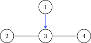
Figure 3: A chain graph representing a non-smooth discrete model under the Alternative Markov Property. (Note that this is not an acyclic directed mixed graph nor a summary graph.)

It follows from Theorem 5.1 that for an ADMG $\mathcal{G}$, the collection of probabilities of the form

$$P(X_{H}={0}\mid X_{T}=x_{T}),\qquad x_{T}\in\mathfrak{X}_{T},H\in\mathcal{H}(\mathcal{G}),$$

is sufficient to recover the joint distribution under the model $\mathcal{P}_{\mathcal{G}}$. However, it is not immediately clear that each of these probabilities is necessary, or more specifically that the map in (2) is smooth and of full rank everywhere.

For brevity, we write $q_{H}(x_{T})\equiv P(X_{H}={0}|X_{T}=x_{T})$, and the vector of all such probabilities by

$$\mathbf{q}\equiv\bigl{(}q_{H}(x_{T})|H\in\mathcal{H}(\mathcal{G}),x_{T}\in\mathfrak{X}_{T}\bigr{)}.$$ (4)

For $\mathbf{p}\in\mathcal{P}_{\mathcal{G}}$, we—in a mild abuse of notation—let $\mathbf{q}(\mathbf{p})$ be the vector of the form (4) determined by calculating the appropriate conditional probabilities from $\mathbf{p}$. Since this only involves adding and dividing strictly positive numbers, the map $\mathbf{q}$ is smooth (infinitely differentiable). Let $\mathcal{Q}_{\mathcal{G}}\equiv\mathbf{q}(\mathcal{P}_{\mathcal{G}})$ be the image of $\mathbf{q}$ over $\mathcal{P}_{\mathcal{G}}$; we call $\mathcal{Q}_{\mathcal{G}}$ the set of derived parameter values. We will prove that the map in (2) provides a smooth inverse to $\mathbf{q}$. The first result shows that the set of vectors ${\mathbf{q}}$ that are derived parameters corresponds exactly to those which give strictly positive probabilities under the inverse map.

Theorem 6.2

For an ADMG $\mathcal{G}$, a vector $\mathbf{q}$ is derived (i.e., $\mathbf{q}\in\mathcal{Q}_{\mathcal{G}}$) if and only if for each $x_{V}\in\mathfrak{X}_{V}$, we have

$$p_{x_{V}}(\mathbf{q})\equiv\sum_{C\dvtx x_{V}^{-1}(0)\subseteq C\subseteq V}(-1)^{|C\setminus x_{V}^{-1}(0)|}\prod_{H\in[C]_{\mathcal{G}}}q_{H}(x_{T})>0,$$ (5)

where $x_{V}^{-1}(0)\equiv\{v\in V|x_{v}=0\}$.

Remark 6.3.

The boundary of $\mathcal{Q}_{\mathcal{G}}$ is the set of $\mathbf{q}$ such that $p_{x_{V}}(\mathbf{q})\geq 0$ for all $x_{V}\in\mathfrak{X}_{V}$, with equality holding in at least one case.

The definition of $p_{x_{V}}(\mathbf{q})$ in (5) is of the same form as the expression given for $P(X_{V}=x_{V})$ in (2) and so the result might at first seem trivial; clearly probabilities must be nonnegative. However, it is not immediately obvious that this condition is sufficient for parameters to be in the image set $\mathcal{Q}_{\mathcal{G}}\equiv\mathbf{q}(\mathcal{P}_{\mathcal{G}})$. If we take some $\mathbf{q}^{\dagger}\notin\mathcal{Q}_{\mathcal{G}}$ and apply to it the nonlinear functional form in (5) to obtain $\mathbf{p}(\mathbf{q}^{\dagger})$, without this result there is no apparent reason why $\mathbf{p}(\mathbf{q}^{\dagger})$ should not be a probability distribution, nor indeed in $\mathcal{P}_{\mathcal{G}}$.

To prove Theorem 6.2, we need the following lemma.

Lemma 6.4

Let $A$ be an ancestral set in $\mathcal{G}$, and let $x_{A}\in\mathfrak{X}_{A}$. Then for any real vector $\mathbf{q}$ (not necessarily in $\mathcal{Q}_{\mathcal{G}}$), the map in (5) satisfies

$$\sum_{y_{V}\dvtx y_{A}=x_{A}}p_{y_{V}}(\mathbf{q}) = \sum_{C\dvtx x_{A}^{-1}(0)\subseteq C\subseteq A}(-1)^{|C\setminus x_{A}^{-1}(0)|}\prod_{H\in[C]_{\mathcal{G}}}q_{H}(x_{T}),$$

where $x_{A}^{-1}(0)\equiv\{v\in A|x_{v}=0\}$. In particular, taking $A=\varnothing$,

$$\sum_{y_{V}}p_{y_{V}}(\mathbf{q})=1.$$

Recall that empty products are assumed equal to 1.

Proof of Lemma 6.4 If $A=V$ the result is trivial. If not, pick some $v\in\operatorname{barren}_{\mathcal{G}}(V)\setminus A$; this is possible because if $A\supseteq\operatorname{barren}_{\mathcal{G}}(V)$ then $A=V$ by ancestrality of $A$. So

$$\mathop{\sum_{y_{V}\dvtx}}_{y_{A}=x_{A}}p_{y_{V}}(\mathbf{q}) = \mathop{\sum_{y_{V}\dvtx}}_{y_{A}=x_{A}}\sum_{y_{V}^{-1}(0)\subseteq C\subseteq V}(-1)^{|C\setminus y_{V}^{-1}(0)|}\prod_{H\in[C]_{\mathcal{G}}}q_{H}(y_{T})$$

$$= \mathop{\sum_{y_{V\setminus\{v\}\dvtx}}}_{y_{A}=x_{A}}\sum_{y_{v}}\sum_{y_{V}^{-1}(0)\subseteq C\subseteq V}(-1)^{|C\setminus y_{V}^{-1}(0)|}\prod_{H\in[C]_{\mathcal{G}}}q_{H}(y_{T})$$

$$= \mathop{\sum_{y_{V\setminus\{v\}\dvtx}}}_{y_{A}=x_{A}}\biggl{(}\sum_{y_{V\setminus\{v\}}^{-1}(0)\subseteq C\subseteq V}(-1)^{|C\setminus y_{V\setminus\{v\}}^{-1}(0)|}\prod_{H\in[C]_{\mathcal{G}}}q_{H}(y_{T})$$

$$\hskip 15.0pt{}+\sum_{y_{V\setminus\{v\}}^{-1}(0)\cup\{v\}\subseteq C\subseteq V}(-1)^{|C\setminus(y_{V\setminus\{v\}}^{-1}(0)\cup\{v\})|}\prod_{H\in[C]_{\mathcal{G}}}q_{H}(y_{T})\biggr{)}.$$

The last equation simply breaks the sum into cases where $y_{v}=1$ and $y_{v}=0$, respectively, which takes this form because $v$ does not appear in any tail sets. The first inner sum in the last expression can be further divided into the cases where $C$ contains $v$, and those where it does not, giving

$$\mathop{\sum_{y_{V}\dvtx}}_{y_{A}=x_{A}}p_{y_{V}}(\mathbf{q}) = \mathop{\sum_{y_{V\setminus\{v\}}\dvtx}}_{y_{A}=x_{A}}\biggl{(}\sum_{y_{V\setminus\{v\}}^{-1}(0)\subseteq C\subseteq V\setminus\{v\}}(-1)^{|C\setminus y_{V\setminus\{v\}}^{-1}(0)|}\prod_{H\in[C]_{\mathcal{G}}}q_{H}(y_{T})$$

$$\hskip 15.0pt{}+\sum_{y_{V\setminus\{v\}}^{-1}(0)\cup\{v\}\subseteq C\subseteq V}(-1)^{|C\setminus y_{V\setminus\{v\}}^{-1}(0)|}\prod_{H\in[C]_{\mathcal{G}}}q_{H}(y_{T})$$

$$\hskip 15.0pt{}+\sum_{y_{V\setminus\{v\}}^{-1}(0)\cup\{v\}\subseteq C\subseteq V}(-1)^{|C\setminus(y_{V\setminus\{v\}}^{-1}(0)\cup\{v\})|}\prod_{H\in[C]_{\mathcal{G}}}q_{H}(y_{T})\biggr{)}.$$

The second and third terms differ only by a factor of $-$1, and so cancel leaving

$$\mathop{\sum_{y_{V}\dvtx}}_{y_{A}=x_{A}}p_{y_{V}}(\mathbf{q}) = \mathop{\sum_{y_{V\setminus\{v\}}\dvtx}}_{y_{A}=x_{A}}\biggl{(}\sum_{y_{V\setminus\{v\}}^{-1}(0)\subseteq C\subseteq V\setminus\{v\}}(-1)^{|C\setminus y_{V\setminus\{v\}}^{-1}(0)|}\prod_{H\in[C]_{\mathcal{G}}}q_{H}(y_{T})\biggr{)}.$$

Repeating this until no vertices outside $A$ are left gives

$$\mathop{\sum_{y_{V}\dvtx}}_{y_{A}=x_{A}}p_{y_{V}}(\mathbf{q}) = \sum_{y_{A}^{-1}(0)\subseteq C\subseteq A}(-1)^{|C\setminus y_{A}^{-1}(0)|}\prod_{H\in[C]_{\mathcal{G}}}q_{H}(y_{T}).$$

In the special case $A=\varnothing$, we end up with an empty product

$$\sum_{y_{V}}p_{y_{V}}(\mathbf{q}) = (-1)^{|\varnothing|}\prod_{H\in[\varnothing]_{\mathcal{G}}}q_{H}(y_{T})=1.$$

Proof of Theorem 6.2 The “only if” part of the statement follows from Theorem 5.1 by the fact that if the parameters are derived then $p_{x_{V}}(\mathbf{q})=P(X_{V}=x_{V})$, and these are therefore positive by definition of $\mathcal{P}_{\mathcal{G}}$.

For the converse, suppose that the inequalities hold; we will show that we can retrieve the parameters simply by calculating the appropriate conditional probabilities. Lemma 6.4 ensures that $\sum_{x_{V}}p_{x_{V}}(\mathbf{q})=1$, and that therefore this is a probability distribution.

Choose some $H^{*}\in\mathcal{H}(\mathcal{G})$, with $T^{*}=\operatorname{tail}_{\mathcal{G}}(H^{*})$ and $A=\operatorname{an}_{\mathcal{G}}(H^{*})$; also set $x_{H^{*}}={0}$ and pick $x_{T^{*}}\in\{0,1\}^{|T^{*}|}$. By Lemma 6.4,

$$\sum_{y_{V}\dvtx y_{A}=x_{A}}p_{y_{V}}(\mathbf{q}) = \sum_{y_{A}^{-1}(0)\subseteq C\subseteq A}(-1)^{|C\setminus y_{A}^{-1}(0)|}\prod_{H\in[C]_{\mathcal{G}}}q_{H}(y_{T}).$$

Now clearly $H^{*}\in\Phi_{\mathcal{G}}(A)$, so applying Lemma 3.4 and the fact that $H^{*}\subseteq x_{A}^{-1}(0)=y_{A}^{-1}(0)$ shows $H^{*}\in[C]_{\mathcal{G}}$ for all terms $C$ in the sum and, therefore, we can apply Proposition 3.5 to factor out the parameter associated with $H^{*}$:

$$= q_{H^{*}}(y_{T^{*}})\sum_{y_{A}^{-1}(0)\subseteq C\subseteq A}(-1)^{|C\setminus y_{A}^{-1}(0)|}\prod_{H\in[C\setminus H^{*}]_{\mathcal{G}}}q_{H}(y_{T})$$

$$= q_{H^{*}}(y_{T^{*}})\sum_{y_{A\setminus H^{*}}^{-1}(0)\subseteq C\subseteq A\setminus H^{*}}(-1)^{|C\setminus y_{A\setminus H^{*}}^{-1}(0)|}\prod_{H\in[C]_{\mathcal{G}}}q_{H}(y_{T}).$$

But note that $A\setminus H^{*}$ is also an ancestral set, and thus using Lemma 6.4 again,

$$\sum_{y_{V}\dvtx y_{A\setminus H^{*}}=x_{A\setminus H^{*}}}p_{y_{V}}(\mathbf{q}) = \sum_{y_{A\setminus H^{*}}^{-1}(0)\subseteq C\subseteq A\setminus H^{*}}(-1)^{|C\setminus y_{A\setminus H^{*}}^{-1}(0)|}\prod_{H\in[C]_{\mathcal{G}}}q_{H}(y_{T}).$$

Hence,

$$\frac{\sum_{y_{V\setminus A}}p_{x_{V}}(\mathbf{q})}{\sum_{y_{V\setminus(A\setminus H^{*})}}p_{x_{V}}(\mathbf{q})} = q_{H^{*}}(x_{T^{*}}),$$

and we can recover the original parameters from the probability distribution $\mathbf{p}$ in the manner we would expect; that $\mathbf{p}$ satisfies the global Markov property for $\mathcal{G}$ then follows from Theorem 5.1. Thus, $\mathbf{p}\in\mathcal{P}_{\mathcal{G}}$ and $\mathbf{q}=\mathbf{q}(\mathbf{p})\in\mathcal{Q}_{\mathcal{G}}$.

Theorem 6.5

For an ADMG $\mathcal{G}$, the model $\mathcal{P}_{\mathcal{G}}$ of strictly positive binary probability distributions satisfying the global Markov property with respect to $\mathcal{G}$ is smoothly parameterized by $\mathbf{q}\in\mathcal{Q}_{\mathcal{G}}$.

Consequently, the model $\mathcal{P}_{\mathcal{G}}$ is a curved exponential family of dimension

$$d=\sum_{H\in\mathcal{H}(\mathcal{G})}|\mathfrak{X}_{\operatorname{tail}(H)}|=\sum_{H\in\mathcal{H}(\mathcal{G})}2^{|\operatorname{tail}(H)|}.$$

By Theorem 6.2, the set $\mathcal{Q}_{\mathcal{G}}\subseteq\mathbb{R}^{d}$ is open. The map $\mathbf{p}(\mathbf{q})\dvtx\mathcal{Q}_{\mathcal{G}}\rightarrow\mathcal{P}_{\mathcal{G}}$ is multilinear and, therefore, infinitely differentiable. Its inverse $\mathbf{q}\dvtx\mathcal{P}_{\mathcal{G}}\rightarrow\mathcal{Q}_{\mathcal{G}}$ is also infinitely differentiable on $\mathcal{P}_{\mathcal{G}}$.

The composition $\mathbf{q}\circ\mathbf{p}$ is the identity function on $\mathcal{Q}_{\mathcal{G}}$ and, therefore, its Jacobian is the identity matrix $I_{d}$. However, the Jacobian of a composition of differentiable functions is the product of the Jacobians, so

$$I_{d}=\frac{\partial\mathbf{q}}{\partial\mathbf{p}}\frac{\partial\mathbf{p}}{\partial\mathbf{q}}.$$

But this implies that each of the Jacobians has full rank $d$ and, therefore, the map $\mathbf{q}$ is a smooth parameterization of $\mathcal{P}_{\mathcal{G}}$. See Kass and Vos (1997), Corollary A.3.

7 Discussion

We remark that it is easy to extend the results of Sections 5 and 6 from the binary case to a general finite discrete state-space; we have avoided this only for notational simplicity. It is also a simple matter to extend the results from ADMGs to the summary graphs of Wermuth (2011) which incorporate three types of edge: directed ($\rightarrow$), undirected ( ), and dashed ( ); the dashed edges are equivalent to bidirected ($\leftrightarrow$) edges [Sadeghi and Lauritzen (2014)]. The undirected component of a summary graph can be dealt with using standard methods for undirected graphs [Lauritzen (1996)], and the remaining parameterization done as for an ADMG, conditional on the undirected component.

Appendix: Technical proofs

Proof of Lemma 4.9 Suppose that two heads $H_{1},H_{2}$ are distinct and $H_{1}\cap H_{2}\neq\varnothing$. We will show that they are dominated by $H^{*}\equiv\operatorname{barren}_{\mathcal{G}}(H_{1}\cup H_{2})$; clearly $H^{*}\subseteq H_{1}\cup H_{2}$ and $H_{1},H_{2}\subseteq\operatorname{an}_{\mathcal{G}}(H^{*})$, so if $H^{*}$ is a head then $\prec$ satisfies the requirements for partition-suitability.

Clearly $H^{*}$ is barren, so we need to prove that it is contained within a single district in $\operatorname{an}_{\mathcal{G}}(H^{*})$. By definition, $\operatorname{an}_{\mathcal{G}}(H^{*})\supseteq H_{1}\cup H_{2}$; we need to find a bidirected path between any $v,w\in H^{*}\subseteq H_{1}\cup H_{2}$. If $v$ and $w$ are either both in $H_{1}$ or both in $H_{2}$, then the existence of such a path follows from the fact that these are heads. If $v\in H_{1}$ and $w\in H_{2}$, then construct a bidirected path in $\operatorname{an}_{\mathcal{G}}(H_{1})$ from $v$ to some vertex $x\in H_{1}\cap H_{2}$, and a bidirected path in $\operatorname{an}_{\mathcal{G}}(H_{2})$ from $x$ to $w$; these paths can then be concatenated into a new path meeting the requirements, shortening the resulting sequence of edges if necessary to avoid repetition of vertices. Hence, $H^{*}$ is a head.

Since $H_{1},H_{2}\subseteq\operatorname{an}_{\mathcal{G}}(H^{*})$ we have $H_{i}\preceq H^{*}$ for each $i=1,2$, and therefore $\prec$ is partition-suitable.

Proof of factorization

Proposition .1

Let $\prec$ and $\prec^{\prime}$ be two partition-suitable partial orderings for $\mathcal{H}$, such that for every $H\in\mathcal{H}$ and $W\subseteq V$, $H$ is maximal in $W$ under $\prec$ whenever this is so under $\prec^{\prime}$. Then $[\cdot]^{\prec}=[\cdot]^{\prec^{\prime}}$.

We again proceed by induction on the size of $W$. Recall that for all $v\in V$, we have $\{v\}\in\mathcal{H}$ by the definition of partition-suitability, so $[\{v\}]^{\prec}=[\{v\}]^{\prec^{\prime}}=\{\{v\}\}$. Now take a general $W\subseteq V$, and suppose that $H$ is maximal under $\prec^{\prime}$ in $W$; then by Proposition 3.5

$$[W]^{\prec^{\prime}} = \{H\}\cup[W\setminus H]^{\prec^{\prime}}$$

$$= \{H\}\cup[W\setminus H]^{\prec}$$

$$= [W]^{\prec}$$

by applying the induction hypothesis to $W\setminus H$, and using the fact that $H\in[W]^{\prec}$ because it is also maximal under $\prec$ in $W$.

Define a partial ordering $\prec^{*}$ on heads in an ADMG by $H_{1}\prec^{*}H_{2}$ if and only if both $H_{1}\prec H_{2}$, and $H_{1}$ and $H_{2}$ are contained in the same district in $\operatorname{an}_{\mathcal{G}}(H_{1}\cup H_{2})$; note that this is a weaker ordering than $\prec$, since strictly fewer pairs of sets are comparable. It is easy to see that $\prec^{*}$ is partition-suitable for heads $\mathcal{H}(\mathcal{G})$ by repeating the proof of Lemma 4.9. In addition, sets which are maximal under $\prec$ will also be maximal under $\prec^{*}$, so the partitions defined by these two orderings are the same by Proposition .1.

This weaker partial ordering leads us to a class of sets which play a role similar to that of ancestral set: a set with “ancestrally closed districts” is one whose districts are ancestrally closed (rather than the whole set).

Definition .2.

Let $\mathcal{G}$ be an ADMG, and $W$ be a subset of its vertices. We say $W$ has ancestrally closed districts if $\operatorname{dis}_{\operatorname{an}(W)}(W)=W$.

Equivalently, $W$ has ancestrally closed districts if $W$ is not connected to $\operatorname{an}_{\mathcal{G}}(W)\setminus W$ by any bidirected edges. This definition is important because the partitioning function $[\cdot]_{\mathcal{G}}$ will act upon sets with ancestrally closed districts “separately” within the relevant ancestral set: that is, for such sets,

$$\bigl{[}\operatorname{an}_{\mathcal{G}}(W)\bigr{]}_{\mathcal{G}}=[W]_{\mathcal{G}}\cup\bigl{[}\operatorname{an}_{\mathcal{G}}(W)\setminus W\bigr{]}_{\mathcal{G}}.$$

Note that if $D=D_{1}\,\dot{\cup}\,D_{2}$ has ancestrally closed districts, and $D_{1}$ and $D_{2}$ are not joined by any bidirected edges, then $D_{1}$ and $D_{2}$ themselves have ancestrally closed districts (here $\dot{\cup}$ indicates a disjoint union). If for every $v,w\in D$ there is a bidirected path from $v$ to $w$ such that all the vertices on the path are contained within $D$, then $D$ cannot be partitioned in this manner, and we say it is bidirected-connected.

Definition .3.

Let $C\subseteq V$. We say that an ordering $<$ on the vertices of $C$ is $(C,\prec^{*})$-consistent if for any $H_{1},H_{2}\in[C]_{\mathcal{G}}$ such that $H_{1}\prec^{*}H_{2}$, we have $v_{1}<v_{2}$ for all $v_{1}\in H_{1}$, $v_{2}\in H_{2}$.

Lemma .4

Let $D=D_{1}\,\dot{\cup}\,D_{2}$ have ancestrally closed districts and be such that $D_{1}$ is not connected to $D_{2}$ by any bidirected edges. Let $<_{1}$ and $<_{2}$ be orderings on $D_{1}$ and $D_{2}$ (resp.). If for $i=1,2$, $<_{i}$ is $(D_{i},\prec^{*})$-consistent, then every extension of $<_{1}$ and $<_{2}$ to an ordering $<$ on $D$ is also a $(D,\prec^{*})$-consistent ordering.

Orderings between vertices $v_{1},v_{2}\in D_{i}$ are specified by $<_{i}$. Further, if $v_{1}\in D_{1}$ and $v_{2}\in D_{2}$ then since $v_{1}$ and $v_{2}$ are in different districts in $\operatorname{an}_{\mathcal{G}}(D)$, it follows from the definition of $\prec^{*}$ that $v_{1}$ and $v_{2}$ can be ordered in any way to achieve a $(D,\prec^{*})$ consistent ordering.

A total ordering $<_{i}$ on a set $D_{i}$ will be said to be topological in $\mathcal{G}$ if no vertex $d\in D_{i}$ precedes any of its proper ancestors in $\mathcal{G}$ that are in $D_{i}$.

Lemma .5

Let $D_{1}$ and $D_{2}$ be disjoint subsets in $\mathcal{G}$. Let $<_{1}$ and $<_{2}$ be topological orderings on $D_{1}$ and $D_{2}$ (resp.). Then there exists an extension of $<_{1}$ and $<_{2}$ to a topological ordering $<$ on $D_{1}\cup D_{2}$.

We construct a topological ordering iteratively as follows: let $\langle d_{1},\ldots,d_{k-1}\rangle$ be the first $k-1$ vertices in $D_{1}\cup D_{2}$ already ordered under $<$; let $E_{k}=(D_{1}\cup D_{2})\setminus\{d_{1},\ldots,d_{k-1}\}$ be the set of vertices remaining to be ordered. Further, let $Q_{k}=\{d\mid d\in E_{k},\operatorname{an}_{\mathcal{G}}(d)\cap E_{k}=\{d\}\}$ be those vertices in $E_{k}$ that have no proper ancestors in $E_{k}$; $Q_{k}\neq\varnothing$ since $V$ is finite and $\mathcal{G}$ is acyclic. Finally, if $Q_{k}\cap D_{1}\neq\varnothing$, define $d_{k}$ to be the first element in $Q_{k}$ under $<_{1}$, otherwise define $d_{k}$ to be the first element in $Q_{k}$ under $<_{2}$. That the ordering is topological follows from the definition of $Q_{k}$.

Lemma .6

Let $D$ have ancestrally closed districts, and suppose $C\subseteq\operatorname{barren}_{\mathcal{G}}(D)$. Then $D\setminus C$ has ancestrally closed districts.

Let $D^{\prime}\equiv D\setminus C$. Since $C\subseteq\operatorname{barren}_{\mathcal{G}}(D)$, $\operatorname{an}_{\mathcal{G}}(D\setminus C)\subseteq\operatorname{an}_{\mathcal{G}}(D)\setminus C$, so

$$\operatorname{dis}_{\operatorname{an}(D^{\prime})}\bigl{(}D^{\prime}\bigr{)}\subseteq\operatorname{dis}_{\operatorname{an}(D)}\bigl{(}D^{\prime}\bigr{)}\setminus C\subseteq\operatorname{dis}_{\operatorname{an}(D)}(D)\setminus C=D\setminus C = D^{\prime}.$$

Since $D^{\prime}\subseteq\operatorname{dis}_{\operatorname{an}(D^{\prime})}(D^{\prime})$, the result holds.

Lemma .7

Let $C\cup W$ have ancestrally closed districts, with $W\subseteq\operatorname{barren}_{\mathcal{G}}(C\cup W)$ and $W\cap C=\varnothing$. Then any ordering on $W$ may be extended to a topological ordering of the vertices in $C\cup W$ which is both $(C,\prec^{*})$ and $(C\cup W,\prec^{*})$-consistent.

Note that $C$ has ancestrally closed districts by Lemma .6. We proceed by induction on the size of $C\cup W$; if $|C\cup W|=0$ or $1$ then the result is trivial.

If $C\cup W$ contains two components which are not connected by bidirected edges, then we can split it into two smaller sets $C_{1}\cup W_{1}$ and $C_{2}\cup W_{2}$, each with ancestrally closed districts, where $C=C_{1}\,\dot{\cup}\,C_{2}$ and $W=W_{1}\,\dot{\cup}\,W_{2}$. Clearly, $W_{i}\in\operatorname{barren}(C_{i}\cup W_{i})$ for each $i$, so using the induction hypothesis, we can find topological orderings $<_{i}$ on the vertices of $C_{i}\cup W_{i}$ which are both $(C_{i}\cup W_{i},\prec^{*})$ and $(C_{i},\prec^{*})$ consistent. It then follows from Lemma .5, taking $D_{i}=(C_{i}\cup W_{i})$, that there exists a topological ordering $<$ on $C\cup W$ that extends $<_{1}$ and $<_{2}$. It further follows from two applications of Lemma .4 that $<$ is both $(C,\prec^{*})$ and $(C\cup W,\prec^{*})$-consistent.

Since, by assumption, $C\cup W$ has ancestrally closed districts, if this set does not contain two components then $C\cup W$ is a single district in$\operatorname{an}_{\mathcal{G}}(C\cup W)$. Let $H=\operatorname{barren}_{\mathcal{G}}(C\cup W)$; this is clearly a head and maximal under $\prec^{*}$ in $C\cup W$. Further, $W\subseteq H$ so applying Proposition 3.5 gives

$$[C\cup W]_{\mathcal{G}} = \{H\}\cup\bigl{[}(C\cup W)\setminus H\bigr{]}_{\mathcal{G}}$$

$$= \{H\}\cup\bigl{[}C\setminus(H\setminus W)\bigr{]}_{\mathcal{G}},$$

since $W\cap C=\varnothing$. Since $H\setminus W\subseteq\operatorname{barren}_{\mathcal{G}}(C)$, Lemma .6 shows that $C\setminus\break(H\setminus W)$ also has ancestrally closed districts; applying the induction hypothesis, we can find a topological ordering of $C$ which is both $(C\setminus(H\setminus W),\prec^{*})$ and $(C,\prec^{*})$-consistent [possibly $C\setminus(H\setminus W)=C$ in which case this is trivial]. This ordering may be combined with an arbitrary ordering on $W$ by simply concatenating the orderings so that everything in $W$ comes after everything in $C$. This gives an ordering which is $(C\cup W,\prec^{*})$-consistent, because $H\supseteq W$ is maximal; since $W$ is barren in $C\cup W$, the ordering is also topological.

Corollary .8

If $D\cup\{w\}$ has ancestrally closed districts with $w\in\operatorname{barren}_{\mathcal{G}}(D\cup\{w\})$, then there exists an ordering $<$ which is both $(D,\prec^{*})$ and $(D\cup\{w\},\prec^{*})$-consistent, and such that $w$ is the maximal vertex under $<$.

The claim is trivial if $w\in D$. Otherwise, $\{w\}$ is barren in $D\cup\{w\}$, so we apply the previous lemma.

Note that the previous lemma and this corollary do not generalize to adding two vertices: there exist graphs with ancestral sets $A$, $A\cup\{w_{1}\}$ and $A\cup\{w_{1},w_{2}\}$, such that no topological ordering is $(A,\prec^{*})$-, $(A\cup\{w_{1}\},\prec^{*})$- and $(A\cup\{w_{1},w_{2}\},\prec^{*})$-consistent. See Richardson (2009) for such an example.

Given a path, $\pi$, and two vertices $v,w$ on $\pi$, the subpath $\pi(v,w)$ is the sequence of edges which lie between $v$ and $w$ on $\pi$. As with a path, we allow a single vertex (and no edges) to be a degenerate case of a subpath.

Lemma .9

Suppose $\pi$ is a path from $a$ to $b$, and is not blocked by $C$. Then every vertex $v$ on $\pi$ is contained in $\operatorname{an}_{\mathcal{G}}(\{a,b\}\cup C)$.

Suppose $w$ is on ${\pi}$ and is an ancestor of neither $a$ nor $b$. Then on each of the subpaths ${\pi}(a,w)$ and ${\pi}(w,b)$, there is at least one edge with an arrowhead pointing towards $w$ along the subpath. Let $v_{aw}$ and $v_{wb}$ be the vertices at which such arrowheads occur that are closest to $w$ on the respective subpaths. There are now three cases: (1) if $w\neq v_{wb}$ then ${\pi}(w,v_{wb})$ is a directed path from $w$ to $v_{wb}$. It further follows that $v_{wb}$ is a collider on ${\pi}$, and since the path is not blocked by $v_{wb}$, it is an ancestor of $C$. Hence, $w\in\operatorname{an}_{\mathcal{G}}(C)$. (2) If $w\neq v_{aw}$, then a symmetric argument holds. (3) If $v_{aw}=w=v_{wb}$, then $w$ is a collider on ${\pi}$, hence again an ancestor of $C$.

The next two lemmas are used to establish necessary results about Markov blankets:

Lemma .10

Let $H_{1},H_{2}\in[D]_{\mathcal{G}}$ with $H_{1}\neq H_{2}$. Then at least one of the following holds: [(iii)]

$H_{1}\prec H_{2}$;

$H_{2}\prec H_{1}$; or

there is no bidirected path between any $h_{1}\in H_{1}$ and $h_{2}\in H_{2}$ contained within $\operatorname{an}_{\mathcal{G}}(H_{1}\cup H_{2})$.

Suppose $H_{1},H_{2}\in[D]_{\mathcal{G}}$, and that (iii) fails. Then let $H^{*}\equiv\operatorname{barren}_{\mathcal{G}}(H_{1}\cup H_{2})$. Since, $H_{1},H_{2}$ are heads and since (iii) fails, $H^{*}$ is a barren set which is connected by bidirected paths in $\operatorname{an}_{\mathcal{G}}(H^{*})=\operatorname{an}_{\mathcal{G}}(H_{1}\cup H_{2})$; hence, it is a head. In addition, $H^{*}\subseteq H_{1}\cup H_{2}\subseteq D$, and $H^{*}\succeq H_{1},H_{2}$.

It follows that $H^{*}\in[D]_{\mathcal{G}}$, which means that either $H^{*}=H_{1}$, in which case (ii) holds, or $H^{*}=H_{2}$, in which case (i) holds.

Lemma .11

Let $D$ be bidirected-connected with ancestrally closed districts, and let $D^{\prime}\equiv D\setminus\{w\}$ for some $w\in\operatorname{barren}_{\mathcal{G}}(D)$. Let $<$ be a total order that is $(D,\prec^{*})$- and $(D^{\prime},\prec^{*})$-consistent, and under which $w$ is maximal. For a given $v\in D^{\prime}$ define $H,H^{\prime}$ to be the heads such that $v\in H\in[D]_{\mathcal{G}}$ and $v\in H^{\prime}\in[D^{\prime}]_{\mathcal{G}}$, respectively, and $T,T^{\prime}$ the corresponding tails. Let

$$B \equiv \bigl{(}\operatorname{dis}_{{\rm Phys.~{}Rev.~{}E}_{<}(v)}(v)\setminus\{v\}\bigr{)}\cup\operatorname{pa}_{\mathcal{G}}\bigl{(}\operatorname{dis}_{{\rm Phys.~{}Rev.~{}E}_{<}(v)}(v)\bigr{)},$$

$$C \equiv \bigl{(}H\cap{\rm Phys.~{}Rev.~{}E}_{<}(v)\bigr{)}\cup T\quad\mbox{and}$$

$$C^{\prime} \equiv \bigl{(}H^{\prime}\cap{\rm Phys.~{}Rev.~{}E}_{<}(v)\bigr{)}\cup T^{\prime}.$$

Then $B\subseteq C$ and $B\subseteq C^{\prime}$, and $B$ m-separates $v$ from both $C\setminus B$ and $C^{\prime}\setminus B$.

Let $S\equiv\operatorname{dis}_{{\rm Phys.~{}Rev.~{}E}_{<}(v)}(v)\subseteq D$; we claim that $S\subseteq\operatorname{an}_{\mathcal{G}}(H)$. If not then there is a bidirected path $\pi$ from $v$ to some $s\in S\setminus\operatorname{an}_{\mathcal{G}}(H)$; let this path be minimal, so that $s$ is adjacent on $\pi$ to some $t\in\operatorname{an}_{\mathcal{G}}(H)$. Then $s$ lies in some different head $H^{*}\in[D]_{\mathcal{G}}$, and we have constructed a bidirected path from $H$ to $H^{*}$ within $\operatorname{an}_{\mathcal{G}}(H\cup H^{*})$; it follows from Lemma .10 that either $H\prec H^{*}$ or $H^{*}\prec H$, but the former is ruled out by the existence of $\pi$ and the $(D,\prec^{*})$-consistency of $<$. Hence, $H^{*}\subseteq\operatorname{an}_{\mathcal{G}}(H)$, and in particular $s\in\operatorname{an}_{\mathcal{G}}(H)$, so we reach a contradiction.

Thus, $S\subseteq\operatorname{an}_{\mathcal{G}}(H)$ and, therefore, $S\equiv\operatorname{dis}_{{\rm Phys.~{}Rev.~{}E}_{<}(v)}(v)\subseteq\operatorname{dis}_{\operatorname{an}(H)}(v)$, so

$$S\cup\operatorname{pa}_{\mathcal{G}}(S)\subseteq\operatorname{dis}_{\operatorname{an}(H)}(v)\cup\operatorname{pa}\bigl{(}\operatorname{dis}_{\operatorname{an}(H)}(v)\bigr{)}\subseteq H\cup T.$$

Finally, using $S\subseteq{\rm Phys.~{}Rev.~{}E}_{<}(v)$, we have

$$B=\bigl{(}S\setminus\{v\}\bigr{)}\cup\operatorname{pa}_{\mathcal{G}}(S)\subseteq\bigl{(}H\cap{\rm Phys.~{}Rev.~{}E}_{<}(v)\bigr{)}\cup T=C.$$

It follows from Lemma .6 and the fact that $w\in\operatorname{barren}_{\mathcal{G}}(D)$, that $D^{\prime}$ also has ancestrally closed districts, and the same argument as above shows that $B\subseteq C^{\prime}$.

Now, let $\pi$ be a path from $v$ to some $c\in C\setminus B$, and assume without loss of generality that $\pi$ does not intersect $C\setminus B$ other than at $c$. We will show that $\pi$ is blocked by $B$.

Note that $B\subseteq C\subseteq{\rm Phys.~{}Rev.~{}E}_{<}(v)$; thus if $\pi$ includes any vertex $s>v$ then it is blocked by Lemma .9, because $s$ is not an ancestor of any element of $C$. Consequently, we may assume that the edge on $\pi$ adjacent to $v$ is of the form $v\leftrightarrow$ or $v\leftarrow$.

We claim that $\pi$ contains at least one non-collider; suppose not for a contradiction: then $\pi$ is of the form

$$v\leftrightarrow t_{1}\leftrightarrow\cdots\leftrightarrow t_{p}\leftrightarrow c,\qquad v\leftrightarrow t_{1}\leftrightarrow\cdots\leftrightarrow t_{p}\leftarrow c\quad\mbox{or}\quad v\leftarrow c,$$

with every node $t_{i}$ an ancestor of $B$ and hence of $D$. Since $D$ has ancestrally closed districts, it follows that every $t_{i}\in D$ and hence $t_{i}\in\operatorname{dis}_{{\rm Phys.~{}Rev.~{}E}_{<}(v)}(v)\setminus\{v\}$, so $t_{i}\in B$. But then $c\in B$, which is a contradiction, since we assumed $c\in C\setminus B$.

It follows that $\pi$ contains at least one non-collider; let $d$ be the non-collider closest to $v$ on the path. But then repeating the argument above (replacing $c$ with $d$) shows that $d\in B$ and, therefore, $\pi$ is blocked by $B$.

Similarly, all paths $\pi^{\prime}$ from $v$ to some $c^{\prime}$ in $C^{\prime}\setminus B$ are blocked by $B$.

The next lemma is the crux of the induction used in the proof of Theorem 4.12.

Lemma .12

Let $D$ have ancestrally closed districts, and $w\in\break\operatorname{barren}_{\mathcal{G}}(D)$. Then for any $f_{V}$ obeying the global Markov property with respect to $\mathcal{G}$, we have

$$\prod_{H\in[D]_{\mathcal{G}}}f_{H|T}(x_{H}|x_{T})=f_{w|\operatorname{an}(D)\setminus\{w\}}(x_{w}|x_{\operatorname{an}(D)\setminus\{w\}})\prod_{H\in[D\setminus\{w\}]_{\mathcal{G}}}f_{H|T}(x_{H}|x_{T})$$

$\mu$-almost everywhere.

Note that we need only prove the case where $D$ forms a single district, from which the general result will follow because by Proposition 3.6 the factors not involving $\operatorname{dis}_{D}(w)$ are the same on both sides. Assume therefore that $D=\operatorname{dis}_{D}(w)$, and thus $D$ is bidirected-connected.

Define $D^{\prime}=D\setminus\{w\}$, and let $<$ be a topological total ordering which is $(D,\prec^{*})$ and $(D^{\prime},\prec^{*})$ consistent, which exists by Corollary .8. Further, we can choose $w$ to be the maximal element in $D$.

For any $v\in H\in[D]_{\mathcal{G}}$, let $H_{v}=H\cap{\rm Phys.~{}Rev.~{}E}_{<}(v)$, and similarly for $v\in H^{\prime}\in[D^{\prime}]_{\mathcal{G}}$, let $H_{v}^{\prime}=H^{\prime}\cap{\rm Phys.~{}Rev.~{}E}_{<}(v)$. In addition, let

$$B_{v}\equiv\bigl{(}\operatorname{dis}_{{\rm Phys.~{}Rev.~{}E}_{<}(v)}(v)\setminus\{v\}\bigr{)}\cup\operatorname{pa}_{\mathcal{G}}\bigl{(}\operatorname{dis}_{{\rm Phys.~{}Rev.~{}E}_{<}(v)}(v)\bigr{)}.$$

Then

$$\prod_{H\in[D]_{\mathcal{G}}}f_{H|T}(x_{H}|x_{T}) = \prod_{H\in[D]_{\mathcal{G}}}\prod_{v\in H}f_{v|H_{v}\cup T}(x_{v}|x_{H_{v}},x_{T})$$

$$= \prod_{H\in[D]_{\mathcal{G}}}\prod_{v\in H}f_{v|B_{v}}(x_{v}|x_{B_{v}})$$

$$= \prod_{v\in D}f_{v|B_{v}}(x_{v}|x_{B_{v}}),$$

where the first equality follows from the elementary properties of conditional probabilities, and the second from applying Lemma .11 to see that $B_{v}$ m-separates $v$ from $(H_{v}\cup T)\setminus B_{v}$.

But $B_{v}$ also m-separates $v$ from $(H^{\prime}_{v}\cup T^{\prime})\setminus B_{v}$, so reversing the argument gives

$$\prod_{v\in D}f_{v|B_{v}}(x_{v}|x_{B_{v}}) = f_{w|B_{w}}(x_{w}|x_{B_{w}})\prod_{v\in D\setminus\{w\}}f_{v|B_{v}}(x_{v}|x_{B_{v}})$$

$$= f_{w|B_{w}}(x_{w}|x_{B_{w}})\prod_{H^{\prime}\in[D\setminus\{w\}]_{\mathcal{G}}}\prod_{v\in H^{\prime}}f_{v|B_{v}}(x_{v}|x_{B_{v}})$$

$$= f_{w|B_{w}}(x_{w}|x_{B_{w}})\prod_{H^{\prime}\in[D\setminus\{w\}]_{\mathcal{G}}}\prod_{v\in H^{\prime}}f_{v|H_{v}^{\prime}\cup T^{\prime}}(x_{v}|x_{H_{v}^{\prime}},x_{T^{\prime}})$$

$$= f_{w|B_{w}}(x_{w}|x_{B_{w}})\prod_{H^{\prime}\in[D\setminus\{w\}]_{\mathcal{G}}}f_{H^{\prime}|T^{\prime}}(x_{H^{\prime}}|x_{T^{\prime}}).$$

In addition, note that $B_{w}=H_{w}\cup T$, so it is the Markov blanket for $w$ in $\operatorname{an}_{\mathcal{G}}(D)$ using the ordered local Markov property. Thus,

$$f_{w|B_{w}}(x_{w}|x_{B_{w}})=f_{w|\operatorname{an}(D)\setminus\{w\}}(x_{w}|x_{\operatorname{an}(D)\setminus\{w\}}),$$

which gives the result.

Proof of Theorem 4.12 We proceed by induction on $|A|$. Clearly, the result holds if $|A|=1$.

If $|A|>1$, then let $w\in\operatorname{barren}_{\mathcal{G}}(A)$; thus $A^{\prime}\equiv A\setminus\{w\}$ is also ancestral. Suppose that the global Markov property holds; then by elementary laws of probability and the induction hypothesis,

$$f_{A}(x_{A}) = f_{w|A^{\prime}}(x_{w}|x_{A^{\prime}})\cdot f_{A^{\prime}}(x_{A^{\prime}})$$

$$= f_{w|A^{\prime}}(x_{w}|x_{A^{\prime}})\prod_{H^{\prime}\in[A^{\prime}]_{\mathcal{G}}}f_{H^{\prime}|T^{\prime}}(x_{H^{\prime}}|x_{T^{\prime}})$$

and by Lemma .12, this is just

$$=\prod_{H\in[A]_{\mathcal{G}}}f_{H|T}(x_{H}|x_{T}).$$

Conversely, suppose that (1) holds and let $<$ be a topological ordering of the ancestral set $A$. By the induction hypothesis, the ordered local Markov property is satisfied for $<$ and all suitable pairs $(v,A^{\prime})$ such that $A^{\prime}\subset A$. Let $w\in\operatorname{barren}_{\mathcal{G}}(A)$ be the maximal vertex under $<$ in $A$, with $H$ such that $w\in H\in[A]_{\mathcal{G}}$; the factorization implies that $H\mathchoice{\mathrel{\hbox to0.0pt{$\displaystyle\perp$\hss}\mkern 2.0mu{\displaystyle\perp}}}{\mathrel{\hbox to0.0pt{$\textstyle\perp$\hss}\mkern 2.0mu{\textstyle\perp}}}{\mathrel{\hbox to0.0pt{$\scriptstyle\perp$\hss}\mkern 2.0mu{\scriptstyle\perp}}}{\mathrel{\hbox to0.0pt{$\scriptscriptstyle\perp$\hss}\mkern 2.0mu{\scriptscriptstyle\perp}}}A\setminus(H\cup T)\mid T$. Note that $H=\operatorname{barren}_{\mathcal{G}}(\operatorname{dis}_{A}(w))$, so

$$\operatorname{mb}_{\mathcal{G}}(w,A) \equiv \bigl{(}\operatorname{dis}_{A}(w)\setminus\{w\}\bigr{)}\cup\operatorname{pa}_{\mathcal{G}}\bigl{(}\operatorname{dis}_{A}(w)\bigr{)}$$

$$= \bigl{(}H\setminus\{w\}\bigr{)}\cup T.$$

This then implies $w\mathchoice{\mathrel{\hbox to0.0pt{$\displaystyle\perp$\hss}\mkern 2.0mu{\displaystyle\perp}}}{\mathrel{\hbox to0.0pt{$\textstyle\perp$\hss}\mkern 2.0mu{\textstyle\perp}}}{\mathrel{\hbox to0.0pt{$\scriptstyle\perp$\hss}\mkern 2.0mu{\scriptstyle\perp}}}{\mathrel{\hbox to0.0pt{$\scriptscriptstyle\perp$\hss}\mkern 2.0mu{\scriptscriptstyle\perp}}}A\setminus(\operatorname{mb}_{\mathcal{G}}(w)\cup\{w\})|\operatorname{mb}_{\mathcal{G}}(w)$ by the weak union property of conditional independence. Hence, the ordered local Markov property is satisfied.

Proof of parameterization

Proposition .13

If $H\in[W]_{\mathcal{G}}$ and $D=\operatorname{dis}_{\operatorname{an}(H)}(H)\cap W$ then $[W]_{\mathcal{G}}=[W\setminus D]_{\mathcal{G}}\cup[D]_{\mathcal{G}}$.

Note that since $H\in[W]_{\mathcal{G}}$, $H\subseteq\operatorname{dis}_{\operatorname{an}(H)}(H)\cap W=D$. The proof is by induction on $|W\setminus D|$. If $W\setminus D=\varnothing$, the claim is trivial. Suppose $H^{*}\in[W]_{\mathcal{G}}$ and $H^{*}\cap D\neq\varnothing$. Applying Lemma .10 to $H,H^{*}\in[W]_{\mathcal{G}}$ we see that either $H^{*}=H$ or $H^{*}\prec H$, so $H^{*}\subseteq D$. Thus, every head in $[W]_{\mathcal{G}}$ is either a subset of $D$ or $W\setminus D$. Consequently, there exists $H^{\dagger}\in[W]_{\mathcal{G}}$ with $H^{\dagger}\subseteq W\setminus D$; let $W^{\dagger}\equiv W\setminus H^{\dagger}$. By Proposition 3.5, $[W]_{\mathcal{G}}=\{H^{\dagger}\}\cup[W^{\dagger}]_{\mathcal{G}}$. Since $D\subseteq W^{\dagger}$ and $H\in[W^{\dagger}]_{\mathcal{G}}$, the conclusion follows from the inductive hypothesis applied to $W^{\dagger}$.

Proof of Lemma 5.4 It suffices to prove the result for $A=V$, from which the general case follows by applying it to the subgraphs $\mathcal{G}_{A}$.

Since $(x_{V},B,W)$ is reducible, $W\setminus B\neq\varnothing$; let $H^{*}$ be a maximal head such that both $H^{*}\in[O\cup W]_{\mathcal{G}}$ and $H^{*}\cap(W\setminus B)\neq\varnothing$, further take $w\in H^{*}\cap(W\setminus B)$. Let $D^{*}\equiv\operatorname{dis}_{\operatorname{an}(H^{*})}(H^{*})$ be the associated district within the ancestors of $H^{*}$. By construction, $D^{*}$ has ancestrally closed districts and is bidirected-connected.

Define $y_{B}\equiv 0$, $y_{V\setminus B}\equiv x_{V\setminus B}$; then

$$g_{x_{V}}(B,W)$$

$$\qquad\equiv(-1)^{|B|}\prod_{H\in[O\cup W]_{\mathcal{G}}}\!P(X_{H}=y_{H}|X_{T}=x_{T})$$

$$\qquad=(-1)^{|B|}\prod_{H\in[(O\cup W)\setminus H^{*}]_{\mathcal{G}}}\!P(X_{H}=y_{H}|X_{T}=x_{T})$$

$$\hskip 132.0pt{}\times\bigl{\{}P(X_{w}=1,X_{{H^{*}}\setminus\{w\}}=y_{{H^{*}}\setminus\{w\}}|X_{T^{*}}=x_{T^{*}})$$

$$\hskip 148.0pt{}+P(X_{w}=0,X_{{H^{*}}\setminus\{w\}}=y_{{H^{*}}\setminus\{w\}}|X_{T^{*}}=x_{T^{*}})$$

$$\hskip 148.0pt{}-P(X_{w}=0,X_{{H^{*}}\setminus\{w\}}=y_{{H^{*}}\setminus\{w\}}|X_{T^{*}}=x_{T^{*}})\bigr{\}}.$$

The last term after distributing the product is just $g_{x_{V}}(B\cup\{w\},W)$, so to prove (3) we need to show that

$$g_{x_{V}}\bigl{(}B,W\setminus\{w\}\bigr{)}$$

$$\qquad\equiv(-1)^{|B|}\prod_{H\in[(O\cup W)\setminus\{w\}]_{\mathcal{G}}}\!P(X_{H}=y_{H}|X_{T}=x_{T})$$

$$\qquad=(-1)^{|B|}$$

(6)

$$\quad\qquad{}\times\prod_{H\in[(O\cup W)\setminus H^{*}]_{\mathcal{G}}}\!P(X_{H}=y_{H}|X_{T}=x_{T})$$

$$\hskip 110.0pt{}\times\bigl{\{}P(X_{w}=1,X_{{H^{*}}\setminus\{w\}}=y_{{H^{*}}\setminus\{w\}}|X_{T^{*}}=x_{T^{*}})$$

$$\hskip 127.0pt{}+P(X_{w}=0,X_{{H^{*}}\setminus\{w\}}=y_{{H^{*}}\setminus\{w\}}|X_{T^{*}}=x_{T^{*}})\bigr{\}}.$$

Note that by the definition of reducibility, $D^{*}\setminus H^{*}\subseteq O\cup(W\setminus B)$, so $D^{*}\setminus H^{*}$ does not contain any “flipped” vertices; hence, $D^{*}\cap B\subseteq H^{*}$. Further, $D^{*}\subseteq O\cup W$.

By Proposition .13, applied to $H^{*}$, $D^{*}$ and $O\cup W$, $[O\cup W]_{\mathcal{G}}=[(O\cup W)\setminus D^{*}]_{\mathcal{G}}\cup[D^{*}]_{\mathcal{G}}$. Thus, every head $H^{\dagger}\in[O\cup W]_{\mathcal{G}}$ which contains a vertex in $D^{*}\setminus H^{*}$ is such that $H^{\dagger}\subseteq D^{*}$. Hence, by applying Lemma .10 to $D^{*}$, it follows that $H^{\dagger}\prec H^{*}$ [since $H^{\dagger}\subseteq D^{*}\setminus H^{*}\subseteq\operatorname{an}_{\mathcal{G}}(H^{*})$ rules out $H^{*}\prec H^{\dagger}$, while $H^{*},H^{\dagger}\subseteq D^{*}$ rules out (iii)]. Thus, $D^{*}$ is made up of $H^{*}$ and the heads which precede it under $\prec$, and hence also under $\prec^{*}$.

Suppose we replace $[O\cup W]_{\mathcal{G}}$ with $[(O\cup W)\setminus S]_{\mathcal{G}}$ for some $S\subseteq H^{*}$; from Lemma 3.4, it is clear that only heads which precede $H^{*}$ under $\prec^{*}$ will be affected, so in particular:

$$\bigl{[}(O\cup W)\setminus H^{*}\bigr{]}_{\mathcal{G}} = \bigl{[}(O\cup W)\setminus D^{*}\bigr{]}_{\mathcal{G}}\cup\bigl{[}D^{*}\setminus H^{*}\bigr{]}_{\mathcal{G}}\quad\mbox{and}$$

$$\bigl{[}(O\cup W)\setminus\{w\}\bigr{]}_{\mathcal{G}} = \bigl{[}(O\cup W)\setminus D^{*}\bigr{]}_{\mathcal{G}}\cup\bigl{[}D^{*}\setminus\{w\}\bigr{]}_{\mathcal{G}}.$$

It follows that to establish (Proof of parameterization) it suffices to show:

$$\prod_{H\in[D^{*}\setminus\{w\}]_{\mathcal{G}}}P(X_{H}=y_{H}|X_{T}=x_{T})$$

$$\qquad=\bigl{\{}P(X_{w}=0,X_{H^{*}\setminus\{w\}}=y_{H^{*}\setminus\{w\}}|X_{T^{*}}=x_{T^{*}})$$

(8)

$$\hskip 3.0pt\quad\qquad{}+P(X_{w}=1,X_{H^{*}\setminus\{w\}}=y_{H^{*}\setminus\{w\}}|X_{T^{*}}=x_{T^{*}})\bigr{\}}$$

$$\quad\qquad{}\times\prod_{H\in[D^{*}\setminus H^{*}]_{\mathcal{G}}}P(X_{H}=y_{H}|X_{T}=x_{T}).$$

Let $z_{D^{*}\setminus\{w\}}\equiv y_{D^{*}\setminus\{w\}}$ and $z_{V\setminus D^{*}}\equiv x_{V\setminus D^{*}}$ (with $z_{w}$ remaining free). Since $D^{*}\cap B\subseteq H^{*}$, applying Lemma .12 to $D^{*}$ and $w$ using the values of $z_{V}$ gives

$$P(X_{w}=z_{w}|X_{(H^{*}\cup T^{*})\setminus\{w\}}=z_{(H^{*}\cup T^{*})\setminus\{w\}})\prod_{H\in[D^{*}\setminus\{w\}]_{\mathcal{G}}}P(X_{H}=z_{H}|X_{T}=z_{T})$$

$$\qquad=\prod_{H\in[D^{*}]_{\mathcal{G}}}P(X_{H}=z_{H}|X_{T}=z_{T})$$

$$\qquad=P(X_{H^{*}}=z_{H^{*}}|X_{T^{*}}=z_{T^{*}})\prod_{H\in[D^{*}\setminus H^{*}]_{\mathcal{G}}}P(X_{H}=z_{H}|X_{T}=z_{T}).$$

Summing both sides of the equation over $z_{w}$ yields (Proof of parameterization). Thus, (3) holds.

It remains to demonstrate that if $B\cup\{w\}\neq W$, the triples $(x_{V},B\cup\{w\},W)$ and $(x_{V},B,W\setminus\{w\})$ are also reducible.

For the first, consider $H\in[O\cup W]_{\mathcal{G}}$ with $H\cap(W\setminus(B\cup\{w\}))\neq\varnothing$. Let $D\equiv\operatorname{dis}_{\operatorname{an}(H)}(H)\subseteq O\cup W$; by construction $D$ has ancestrally closed districts. Since $H\cap(W\setminus B)\supseteq H\cap(W\setminus(B\cup\{w\}))\neq\varnothing$, by the reducibility of $(x_{V},B,W)$, $D\setminus H\subseteq O\cup(W\setminus B)$. It is sufficient to show that $w\notin D\setminus H$. Since by Proposition .13, $[O\cup W]_{\mathcal{G}}=[(O\cup W)\setminus D]_{\mathcal{G}}\cup[D]_{\mathcal{G}}$, if $w\in D\cap H^{*}$ then $H^{*}\in[D]_{\mathcal{G}}$. If $H=H^{*}$, then $w\notin D\setminus H$. If $H\neq H^{*}$, then applying Lemma .10 we have $H^{*}\prec H$ (by the same argument as above). But this contradicts that $H^{*}$ is a maximal head in $[O\cup W]_{\mathcal{G}}$ such that $H^{*}\cap(W\setminus B)\neq\varnothing$. Hence, $(x_{V},B\cup\{w\},W)$ is reducible.

We now consider $(x_{V},B,W\setminus\{w\})$. Let $H\in[O\cup(W\setminus\{w\})]$, with $H\cap((W\setminus\{w\})\setminus B)\neq\varnothing$. Again, let $D\equiv\operatorname{dis}_{\operatorname{an}(H)}(H)$.

First suppose $H\in[(O\cup W)\setminus D^{*}]_{\mathcal{G}}$ then, by (Proof of parameterization), $H\in[O\cup W]_{\mathcal{G}}$. We showed above that if $H\in[O\cup W]_{\mathcal{G}}$ and $H\cap(W\setminus(B\cup\{w\}))\neq\varnothing$ then $D\setminus H\subseteq(W\setminus(B\cup\{w\}))$. This is sufficient since $W\setminus(B\cup\{w\})=(W\setminus\{w\})\setminus B$.

If $H\notin[(O\cup W)\setminus D^{*}]_{\mathcal{G}}$ then (Proof of parameterization) implies $H\in[D^{*}\setminus\{w\}]_{\mathcal{G}}$. Lemma .6 applied to $D^{*}$ implies that $D^{*}\setminus\{w\}$ has ancestrally closed districts, so $D\subseteq D^{*}\setminus\{w\}$. Since $D\subseteq D^{*}$, if a vertex $v$ is not barren in $D$ then $v\notin\operatorname{barren}_{\mathcal{G}}(D^{*})=H^{*}$. Hence, $H^{*}\cap D\subseteq\operatorname{barren}_{\mathcal{G}}(D)=H$. Thus,

$$D\setminus H\subseteq D\setminus H^{*}\subseteq D^{*}\setminus H^{*}\subseteq O\cup(W\setminus B),$$

where the third inclusion follows from the reducibility of $(x_{V},B,W)$ and the choice of $H^{*}$. But since $D\subseteq D^{*}\setminus\{w\}$, we have $D\setminus H\subseteq O\cup((W\setminus\{w\})\setminus B)$ as required.

References

• Andersson, Madigan and Perlman (2001) {barticle}[mr] \bauthor\bsnmAndersson, \bfnmSteen A.\binitsS. A., \bauthor\bsnmMadigan, \bfnmDavid\binitsD. and \bauthor\bsnmPerlman, \bfnmMichael D.\binitsM. D. (\byear2001). \btitleAlternative Markov properties for chain graphs. \bjournalScand. J. Stat. \bvolume28 \bpages33–85. \biddoi=10.1111/1467-9469.00224, issn=0303-6898, mr=1844349 \bptokimsref\endbibitem
• Bartolucci, Colombi and Forcina (2007) {barticle}[mr] \bauthor\bsnmBartolucci, \bfnmFrancesco\binitsF., \bauthor\bsnmColombi, \bfnmRoberto\binitsR. and \bauthor\bsnmForcina, \bfnmAntonio\binitsA. (\byear2007). \btitleAn extended class of marginal link functions for modelling contingency tables by equality and inequality constraints. \bjournalStatist. Sinica \bvolume17 \bpages691–711. \bidissn=1017-0405, mr=2398430 \bptokimsref\endbibitem
• Bergsma and Rudas (2002) {barticle}[mr] \bauthor\bsnmBergsma, \bfnmWicher P.\binitsW. P. and \bauthor\bsnmRudas, \bfnmTamás\binitsT. (\byear2002). \btitleMarginal models for categorical data. \bjournalAnn. Statist. \bvolume30 \bpages140–159. \biddoi=10.1214/aos/1015362188, issn=0090-5364, mr=1892659 \bptokimsref\endbibitem
• Dawid (1979) {barticle}[mr] \bauthor\bsnmDawid, \bfnmA. P.\binitsA. P. (\byear1979). \btitleConditional independence in statistical theory. \bjournalJ. Roy. Statist. Soc. Ser. B \bvolume41 \bpages1–31. \bidissn=0035-9246, mr=0535541 \bptnotecheck related \bptokimsref\endbibitem
• Dawid and Didelez (2010) {barticle}[mr] \bauthor\bsnmDawid, \bfnmA. Philip\binitsA. P. and \bauthor\bsnmDidelez, \bfnmVanessa\binitsV. (\byear2010). \btitleIdentifying the consequences of dynamic treatment strategies: A decision-theoretic overview. \bjournalStat. Surv. \bvolume4 \bpages184–231. \biddoi=10.1214/10-SS081, issn=1935-7516, mr=2740837 \bptokimsref\endbibitem
• Drton (2009) {barticle}[mr] \bauthor\bsnmDrton, \bfnmMathias\binitsM. (\byear2009). \btitleDiscrete chain graph models. \bjournalBernoulli \bvolume15 \bpages736–753. \biddoi=10.3150/08-BEJ172, issn=1350-7265, mr=2555197 \bptokimsref\endbibitem
• Drton and Xiao (2010) {bincollection}[mr] \bauthor\bsnmDrton, \bfnmMathias\binitsM. and \bauthor\bsnmXiao, \bfnmHan\binitsH. (\byear2010). \btitleSmoothness of Gaussian conditional independence models. In \bbooktitleAlgebraic Methods in Statistics and Probability II. \bseriesContemp. Math. \bvolume516 \bpages155–177. \bpublisherAmer. Math. Soc., \blocationProvidence, RI. \biddoi=10.1090/conm/516/10173, mr=2730747 \bptokimsref\endbibitem