Correlations between SDSS Type Ia Supernova Rates and Host Galaxy Properties

Abstract

Studying the correlation of type Ia supernova rates (SNR) with host galaxy properties is an important step in understanding the exact nature of type Ia supernovae. We use SNe Ia from the SDSS-II sample, spectroscopically determined masses and star formation rates, and a new maximum likelihood method, to fit the Scannapieco and Bildsten rate model $SNR=A{\times}M+B{\times}SFR$, where $M$ is galaxy mass and $SFR$ is star formation rate. We find $A=3.5^{+0.9}_{-0.7}\times 10^{-14}(\text{SNe/yr})(M_{\odot})^{-1}$ and $B=1.3^{+0.4}_{-0.3}\times 10^{-3}(\text{SNe/yr})(M_{\odot}$yr${}^{-1})^{-1}$, assuming overall efficiency of 0.5. This is in reasonable agreement with other determinations. However we find strong evidence that this model is a poor fit to other projections of the data: it fails to correctly predict the distribution of supernovae with host mass or SFR. An additional model parameter is required; most likely this parameter is related to host galaxy mass. Some implications of this result are discussed.

1. Introduction

Supernovae of type Ia (SNe Ia) played a pivotal role in the discovery of the accelerating Universe (Riess et al. 1998, Perlmutter et al. 1999), and are among the most reliable standard candles on cosmological distance scales (Sullivan et al. 2011, Barone-Nugent et al. 2012). However, a complete understanding of SN Ia progenitor systems has yet to be achieved, even though credible models for such progenitors exist (e.g. Hillebrandt & Niemeyer 2000, Nomoto 1982, Hachisu et al. 1996). Many methods have been developed to discriminate between proposed models, including the theoretical modelling of progenitor systems (e.g., Han & Podsiadlowski 2006, Wang et al. 2010), and the measurement of delay time distributions (e.g., Mennekens et al. 2010, Totani et al. 2009, Sand et al. 2012; Maoz et al. 2012; see also Greggio 2005, 2010).

One approach used in constraining the nature of SNe Ia progenitors is studying the correlation between SN Ia rates (SNR) and the properties of the galaxies in which they form (e.g., Maoz & Mannucci 2011). The environmental properties studied so far include redshift (e.g., Dilday 2010a and 2010b), host galaxy age (e.g., Gupta et al. 2011), environment galaxy number density (e.g., Cooper et al. 2009), ejecta velocity (e.g., Foley 2012), and, most relevant to this work, mass and star formation rate of the host (e.g., Sullivan et al. 2006).

In this paper, we investigate the correlation between SN Ia rates and the mass and star formation rate of the host galaxies in which they formed. One popular model for this correlation is the “$A+B$” model (Scannapieco & Bildsten 2005), which states that the supernova rate is proportional to a linear combination of galaxy mass and star formation rate: $SNR=A{\times}M+B{\times}SFR$, where $SNR$ is the SN Ia rate, $M$ is galaxy mass in stars, and $SFR$ is star formation rate. This relation leads trivially to a more physical relation $SNR/M=A+B{\times}(SFR/M)$, where $SNR/M$ is the rate per unit mass, and $SFR/M$ is specific star formation rate (which is a function of star formation history, independent of mass).

Substantial effort has been invested in determining the values of $A$ and $B$ since the work of Scannapieco and Bildsten (2005). See Fig. 1 for a comparison of some of these results. Neill et al. (2006) and Dilday et al. (2008) used volumetric SN Ia rates to infer these parameters. Of particular interest is the work of Sullivan et al. (2006), who obtained stellar masses and SFRs of each individual host (and field) galaxy by fitting PEGASE2 spectral templates to multiband photometry (Fioc & Rocca-Volmerange 1997, Le Borgne and Rocca-Volmerange 2002). They concluded that $A=5.3\pm 1.1\times 10^{-14}(\text{SNe/yr})(M_{\odot})^{-1}$, $B=3.9\pm 0.7\times 10^{-4}(\text{SNe/yr})(M_{\odot}$yr${}^{-1})^{-1}$, values that we will return to.

On the other hand, Smith et al. (2012) used photometric masses and SFR’s to demonstrate that the $A+B$ model was not a good match to SDSS-II supernova data (Frieman et al. 2008). They proposed an alternate model of the form $SNR=A{\times}M^{x}+B{\times}SFR^{y}$, with $x\simeq 0.7$ and $y\simeq 1$. This is, on the surface, broadly consistent with the mass dependence found by Li et al. (2011) from the Lick Observatory Supernova Survey (LOSS) (though see §6).

The primary objective of this work is to obtain fits to SNR models using spectroscopically-determined masses and SFRs from the SDSS DR7 MPA/JHU value-added catalog (Kauffmann et al. 2003, Brinchmann et al. 2004, Tremonti et al. 2004), making these values somewhat independent of, and possibly more reliable than, those based on multiband photometric data. This is of significance since it has been pointed out (e.g., Förster et al. 2006) that the uncertainty in measurements of star formation histories is an important limiting factor in the determination of the values of $A$ and $B$. In addition, we use a new fitting algorithm for $A$ and $B$ based on maximum likelihood, which is more reliable than previous fitting methods.

In §2, we present the data samples we use in our studies, which include the sample of SNe Ia, the sample of photometric galaxies, and the subset of spectroscopic galaxies (itself a subset of the photometric sample). Also presented in §2 is the essential preprocessing of the data, most notably the matching of the SNe Ia to their host galaxies in the photometric sample, and a brief introduction to the MPA/JHU masses and SFRs, in addition to a comparison with other masses and SFRs. Our results for $A$ and $B$ are given in §3, and a detailed examination of the fit of the model to the data is given in §4. Finally we discuss alternate models in §5, and the implications of these alternate models in §6.

2. Data

The Sloan Digital Sky Survey (SDSS, Abazajian et al. 2009) Data Release 7 catalog (DR7) contains 357 million unique objects, of which nearly 930,000 are galaxies for which spectra are available. From these spectra, masses and star formation rates have been obtained (Kauffmann et al. 2003, Brinchmann et al. 2004, Tremonti et al. 2004, hereafter MPA/JHU); see §2.2 for details. Supernova identifications were taken from the SDSS-II Supernova Survey, which is a 3-year (2005-2007) survey conducted within Stripe 82 of the SDSS. Stripe 82 covers an area of nearly 300 square degrees in a belt along the celestial equator, and contains $\sim$20,000 of the spectroscopic galaxies mentioned above. For each year the survey was conducted, supernova imaging was conducted for 3 months, resulting in a total observation period of 9 months.

2.1. SDSS II Type Ia Supernovae

From the complete sample of 660 SDSS II supernovae (Frieman et al. 2008), we extract 520 spectroscopically confirmed SNe Ia, 503 of which were observed during the 3 observation seasons in 2005, 2006 and 2007. (For the rest of this paper, “SNe” refers to SNe Ia unless stated otherwise.) Our sample is larger than that used by Smith et al. (2012), since we include SNe within $z=0.05$. We omit 17 SNe observed in 2004, since the observation windows and completeness of these SNe would be hard to gauge.

Dilday et al. (2008, 2010) have shown that the identification efficiency $\epsilon_{z}$ in the SDSS-II Supernova Survey is $\gtrsim 0.7$ out to a redshift of 0.15, and $>$0.5 out to z=0.25 (e.g. Fig. 8 of Dilday et al. 2010). In fact the median z of SN in our (spectroscopic host) sample is much lower ($\langle z\rangle=0.11$) than for the SDSS SN Ia sample as a whole ($\langle z\rangle=0.2$) because of the severe magnitude limit $r=17.77$ for the spectroscopic sample of hosts. Thus incompleteness $\epsilon_{z}=0.7$ appears to be a reasonable assumption. We also assume an observation window $T=9$ months in length, and detection efficiency $\epsilon_{t}=1$. The size of the SN sample is therefore assumed to be the intrinsic number occuring in the sky within a timeframe of $\epsilon_{t}\epsilon_{z}T=0.5$ year. This assumption is discussed further in §6.1, but we note here that different values of $\epsilon_{t}\epsilon_{z}T$ result in a simple scaling of supernova rates, and hence of $A$ and $B$ values.

2.2. SDSS Spectroscopic Masses and Star Formation Rates

The SDSS DR7 MPA/JHU value-added catalog contains derived masses and SFR values for the spectroscopic galaxies, including 19987 galaxies in Stripe 82 (our spectroscopic sample). The mass estimates follow a methodology similar to that of Kauffmann et al. (2003), namely a grid search over a library of star formation histories (Bruzual & Charlot 2003) for the most probable mass-to-light ratio. (This is slightly different from the approach of Kauffmann et al. (2003), which matches $D_{n}(4000)$ and $H\delta_{A}$, but it has been shown that the mass estimates of the two methods do not differ by more than $\sim 0.1$dex.) The methods used for obtaining SFR measurements were similar to those proposed by Brinchmann et al. (2004). Galaxies were divided into three classes: (1) “SF”, (2) “low S/N SF”, and (3) “AGN, Composite and Unclassifiable”. The “SF” class was processed by fitting 5 emission lines ($H_{\alpha}$, $H_{\beta}$, O III, N II and S II) to those of simulated galaxies in a spectral library obtained using the code by Charlot & Longhetti (2001). For the “low S/N SF” class, Brinchmann et al. used a simple conversion factor between attenuation-corrected $H_{\alpha}$ luminosity and SFR. The “AGN, Composite and Unclassifiable” class was processed by means of the empirical relation between SFR and D4000.

One problem with this methodology is that passive galaxies are always assigned a (very small) SFR. This can be seen in Fig. 2, where MPA/JHU spectroscopic galaxies are plotted in the mass-SFR plane. It is demonstrated in §4 that this does not significantly affect our results.

To test the reliability of the MPA/JHU masses and SFR’s, we compare their results with those of the VESPA catalogue (Tojeiro et al. 2009), which estimates the star formation history of a number of galaxies in SDSS Stripe 82 using spectroscopic methods. VESPA masses are obtained by summing the star formation history; VESPA SFR’s are obtained from a SFH averaged over the redshift range 0 to 0.11. A comparison of these quantities with their MPA/JHU counterparts is made in Fig. 3. From this figure, it can be seen that the mass and SFR estimates from the two catalogues are in reasonable agreement with each other, with offsets of 0.25 and 0.24 for log M and log SFR, and rms scatter of 0.18 dex and 0.48 dex, respectively.

At this point it is relevant to ask how much better spectroscopically-determined masses and star formation rates are than their photometric counterparts (as used by, for example, Sullivan et al. 2006, and Smith et al. 2012). The advantage of using spectroscopic data is due to several effects. 1. Redshift estimates (required for both the SN and field samples – e.g., §3) are much better for spectroscopic data. Using the same sample as ours, Smith et al. (2012) showed that photometric redshifts result in negligible offsets (0.03 dex) but a scatter of $>0.2$ dex in log M and log SFR relative to using spectroscopic redshifts. 2. Photometric methods for obtaining M and SFR from SDSS data rely on fitting evolving stellar population models to 5 broad photometric bands. The simplicity of these models, coupled with the wide range of degeneracies between model parameters, will result in larger random errors, particularly for SFR. By comparison spectroscopic methods allow the use of far more data, including emission lines, absorption lines, and spectral breaks that are better tuned to the determination of M and SFR. 3. From a comparison of two different catalogs above, we have already seen that there are significant systematics in the determination of spectroscopic M and SFR. For all the reasons mentioned in point 2, there are likely to be even larger systematic errors in photometric M and SFR measurements. These systematics are of the greatest concern; none of our conclusions are affected by random errors in M and SFR.

2.3. Host Matching

We adopt the host matching algorithm of Sullivan et al. (2006). We use SDSS DR7 $r$ band data to calculate a dimensionless parameter $R_{25}$ for every potential host - SN pair. $R_{25}$ is the angular separation of a SN from its prospective host, measured in units of the size of the 25 magnitudes/arcsec² isophote, and allowing for the shape of this isophote (see Fig. 4). The host candidate is then identified to be the galaxy with the lowest $R_{25}$. SNe Ia with redshifts falling more than $3\sigma$ from the photometric redshift of the host galaxy are then discarded. Using such a selection procedure, for hosts with spectroscopy, host z and SN z are always in agreement to a precision of 0.001.

How large can $R_{25}$ be without introducing significant contamination? To answer this question, we conducted Monte Carlo simulations with randomly distributed artificial SN positions, keeping in mind that a majority of contamination is due to SNe for which the host is not seen. We find that the contamination is $\sim$ 8% when only SN-host candidate pairs with $R_{25}<3.8$ are identified as genuine matches. Contamination could be larger if we were to take clustering effects into account, but such effects are hard to quantify. Applying this criterion, we find 351 matches for the SNe within the SDSS DR7 database. Of these, 53 are galaxies in the spectroscopic sample, with MPA/JHU masses and SFRs. It may be argued that since $\sim$ 170 SNe were unmatched, $\sim$ $8\%\times 170\sim 14$ SNe of the 351 could be random matches. We consider this number to be relatively small in comparison to the 351 matches. Also, this contamination estimate corresponds to the expected contamination from using $R_{25}$ alone as matching criteria. The additional redshift constraints would help further lower the number of random matches. The question of contamination is re-examined in §6.2.

To test the host-matching procedure above, we use 2 separate methods. The first is to visually examine the images of the SN - host pairs, relative to their $R_{25}=1$ isophotes. The second is to plot the number of SN matches versus the $R_{25}$ criterion adopted (Fig. 5). We can see that there is a flat region beyond $R_{25}=3.8$, which we assume to be the regime where random matches between SNe and non-host galaxies become dominant.

We also compare the discrepancies between our host-matching method and the “closest angular distance” matching method used by many other authors (e.g. McGee and Balogh 2010). We find that the two matching methods give different results for $\sim$10% of the SNe.

3. Fitting $A$ and $B$

We adopt a fitting algorithm based on maximum likelihood. Using Poisson probabilities, the likelihoods of a galaxy hosting/not hosting a SN Ia are

$$P(S_{i}|SN)=S_{i}e^{-S_{i}},\text{\ and\ }P(S_{i}|\overline{SN})=e^{-S_{i}},\\$$ (1)

where $S_{i}$ is the expected SN Ia rate for each galaxy within our observing window, calculated for every galaxy individually by means of the mass and SFR data. (None of the hosts in our sample hosted more than one SN.) Multiplying these likelihoods for every galaxy, we obtain a log likelihood of obtaining our dataset of

$${\rm ln}L=-\displaystyle\sum_{n=1}^{19987}S_{n}+\displaystyle\sum_{m=1}^{53}({\rm ln}S_{m})+\text{constant}.$$ (2)

where 53 is the number of galaxies hosting SNe, and 19987 is the total number of galaxies in our Stripe 82 spectroscopic sample.

We perform a grid search to find the maximum likelihood $A$ and $B$ values, which are $A=3.5^{+0.9}_{-0.7}\times 10^{-14}(\text{SNe/yr})(M_{\odot})^{-1}$ and $B=1.3^{+0.4}_{-0.3}\times 10^{-3}(\text{SNe/yr})(M_{\odot}$yr${}^{-1})^{-1}$. Fig. 6 plots the probability contours and error bars for our grid search, while Fig. 7 compares these results with the observed SNR at different specific SFR (where specific SFR $sSFR=SFR/M$)

While exceptionally simple, the maximum likelihood analytical method above does have the drawback that it neglects statistical uncertainties in the determination of M and SFR. The method could be modified to include the effects of these uncertainties, however, given our conclusion (§4) that the A+B model is not valid, we have chosen instead to simply simulate the effects of these uncertainties. We have conducted a set of Monte Carlo simulations by seeding random, artificial SNe into the spectroscopic sample, and have included the effects of uncertainties in M and SFR. We find that A and B are biased by +0.05 and -0.05 when the effects of uncertainties in M and SFR are included. (This bias is in the sense “derived value minus true value”.) The mass term and the SFR term contribute 27 and 26 SNe Ia respectively, implying that there are as many prompt SNe Ia as delayed SNe Ia according to the model.

Our final results ($A=3.5^{+0.9}_{-0.7}\times 10^{-14}(\text{SNe/yr})(M_{\odot})^{-1}$ and $B=1.3^{+0.4}_{-0.3}\times 10^{-3}(\text{SNe/yr})(M_{\odot}$yr${}^{-1})^{-1}$) are consistent within error bars with most of the literature. For a summary/comparison of these results, see Fig. 1.

4. Inconsistencies in the $A+B$ Model

The $A$ and $B$ values above are optimal in a maximum likelihood sense. However, there is no guarantee that the $A+B$ model provides a good fit to our data; more tests are needed.

As a test of the $A+B$ model’s consistency, we rank the spectroscopic galaxy sample of 19987 galaxies by mass, calculate the cumulative percentage distribution of SNR for both the $A+B$ model and the observations, and apply a Kolmogorov-Smirnov (K-S) test to the two distributions (Fig. 8). The $A+B$ model with our derived values for $A$ and $B$ is rejected at the 99% confidence level. This result was also found by Smith et al. (2012).

To investigate the possibility that other $A$ and $B$ values could have passed the test, we plot (Fig. 8) the cumulative distribution functions of our galaxies for both an $A$-only model (SNR=$A{\times}$M) and a $B$-only model (SNR=$B{\times}$SFR), keeping in mind that any set of values of $A$ and $B$ must fall between these two distributions. (Note that for the $A$-only and $B$-only models, the values taken for $A$ and $B$ do not affect the result of the K-S test.) The $A$-only model is rejected at an even higher degree, while the $B$-only model passes the test ($\sim$ 50% rejection). This shows that our data do not support a larger value of $A$/$B$.

Passing the mass-ranked K-S test is a necessary but insufficient condition for a SNR model to be plausible. Almost all models pass the sSFR-ranked K-S tests, including the $A+B$ model (Fig. 9), but the same cannot be said for the SFR-ranked K-S tests, for which both the generic $A+B$ model, the $B$-only model, and all models in between are rejected (Fig. 10). This means that a smaller value of $A$/$B$ will not pass the test. Since we already know that a larger $A$/$B$ value will not work (see above), we conclude from these tests that no $A+B$ model can match our observed data. The results of these KS tests are shown in Table 2.

The KS test is usually valid only when the measurement uncertainties in the observed sample are small. Therefore the (possibly significant) uncertainties in the mass and SFR measurements brings the validity of our above methods into question. In order to check the validity of our K-S test under such conditions, we use a Monte Carlo approach. We generate many artificial samples of supernovae using the best fit A and B values with the sample of 19987 observed M and SFR values, add the effects of uncertainties in M and SFR, and generate cumulative distributions of log M and log SFR. The results are completely consistent with the K-S tests: the A+B model is rejected at $>$99% probability for log M and $>$97% probability for log SFR.

The maximum likelihood method for fitting A and B returns a probability which can be used as a measure of goodness of fit. This probability can be interpreted using Monte Carlo simulations. Allowing for the fact that this probability depends on the number of supernovae generated (which varies from run to run), we find that more than 99.9% of all simulations possess a peak probability greater than that of the best fit to the observations. Thus we conclude, independently of the K-S tests, that the A+B model is not a good match to the data.

To present an alternate, and somewhat more illustrative, view of this discrepancy, we separate the galaxies by mass into two equally-sized groups divided at log M=10.7, and plot specific SNR vs. specific SFR (as in Fig. 6 of Sullivan et al. 2006). The resulting plot (Fig. 11) shows that low-mass galaxies have a systematically higher specific SNR than their high-mass counterparts, by a factor of 3–5. Applying different mass cuts consistently results in the same trend.

A plot of the differential distribution functions of SNR predicted by the $A+B$ model vs the actual observed SNR (Fig. 12) further illustrates the issue, where the curves have been scaled to show the relative absolute SNR obtained by each model. From Fig. 12, it can be seen that both the predictions of our best-fit $A+B$ model (green line) and that of Sullivan et al. (2006) (blue line) underpredict the rates of supernovae hosted by low mass, high specific star formation rate galaxies, while overpredicting the rates in high mass galaxies. The red line is a (somewhat unphysical) modified $A+B$ model with a constant background supernova rate added (§4.1). The two (unmodified) $A+B$ models are in reasonable agreement with each other.

To show how large an effect our uncertainties in the determination of the $A$ and $B$ parameters may have on Fig. 12, we plot Fig. 13, which shows the differential distributions for the 1$\sigma$ upper and lower limits for $A$ and $B$. It can be seen that the uncertainties cannot account for the discrepancy at the low mass end.

As mentioned in §2, the MPA/JHU catalog systematically overestimates the SFRs of passive (non-star-forming) galaxies, assigning them a small but significant SFR. We redo the $A+B$ fits by setting the SFRs of all galaxies with an sSFR smaller than $10^{-11.5}$ $(M_{\odot}/\mathrm{yr})/M_{\odot}$ to zero; our results are unaffected.

5. Modifications to the $A+B$ Model

We have demonstrated that the $A+B$ model does not reproduce our data. To account for the discrepancy, most notably the observed SNR excess in low mass galaxies, we now try modifications to the $A+B$ model. Table 2 summarizes the results for some of the many models tried. Due to our small sample size, and also to intrinsic uncertainties in the MPA/JHU measurements of masses and star formation rates, there exist strong correlations between model parameters when more than 2 parameters are used.

As previously found by Sullivan et al. (2006), $A\times M$- and $B\times SFR$-only models do not match the observed SNR distributions. The $A{\times}M+B{\times}SFR+C$ and $(A{\times}M+B{\times}SFR)(1+C{\times}M^{-1})$ models are particularly interesting, since they both pass the KS tests, and might have a physical explanation (§6).

We also investigate the model proposed by Smith et al. (2012): $SNR=A{\times}M^{x}+B{\times}SFR^{y}$. We attempt to obtain best-fit values for the parameters of our own using maximum likelihood, but find that our sample is too small to overcome the correlations between 4 parameters. Using Smith et al.’s values of $x=0.72$, and $y=1.01$, we refit $A$ and $B$ using maximum likelihood; the result is $A=5.3^{+1.3}_{-0.9}\times 10^{-11},B=1.0^{+0.4}_{-0.3}\times 10^{-3}$ (appropriate units in the $M_{\odot}$ - yr system). Using either these values, or the $A$ and $B$ values given by Smith et al. ($A=0.41\times 10^{-10},B=0.65^{\times}10^{-3}$), we find that the model passes the mass-ranked test, but fails the SFR-ranked test at 99% confidence. A very small value of $x=0.06\pm 0.10$ fits the data better, and passes both KS tests - this is probably a manifestation of the C term mentioned above.

6. Discussion

In this paper, we have obtained $A$ and $B$ values from spectroscopic data. However, further analysis reveals that there is an intrinsic inconsistency between the data and the $A+B$ model: mass-ranked KS tests reject all $A$ and $B$ values with a higher $A$/$B$ ratio than our best-fit values, while SFR-ranked KS tests reject those with a smaller $A$/$B$ ratio; furthermore, from Figs. 8, 11 and 12, we can see that there exists a SNR excess in low mass galaxies. §6.1 discusses some possible issues with the data and its interpretation; §6.2 interprets our results.

6.1. Data Issues

We have not applied any completeness corrections to the supernovae. The completeness of the sample has been discussed in §2; incompleteness will affect the numerical values of $A$ and $B$ by less than 0.1 dex, but will not affect $A$/$B$, nor any of the conclusions regarding the $A+B$ model (unless there is strong redshift evolution in the SNR – something that is not observed – e.g., Perrett et al. 2012). To check this, we redo the work with a redshift cut of 0.20 instead of 0.25, and find no significant differences.

Is it possible that the detection efficiency is different in galaxies with high star formation, and concomitant higher extinction? We have already noted that the detection efficiency of our sample is higher than for SDSS SNe as a whole (§2.1). In fact high specific SFR implies lower M and luminosity (Brinchmann et al. 2004) and as a result the star forming galaxies (log sSFR $>-10.5$) in our sample have an even lower mean z (about 0.07); this means that incompleteness is even less of a problem. A simulation of an extreme efficiency variation with sSFR shows that, while $B$ will be biased, the main conclusion regarding the inapplicability of the $A+B$ model remains unaltered.

The precision of the SDSS MPA/JHU masses and star formation rates may affect our conclusions. We have already mentioned the effects of statistical uncertainties in the derived M and SFR quantities. We repeat our work using VESPA masses and star formation rates. The resulting values of $A$ and $B$ conform better to those found by Sullivan et al. (2006) (see Table 1), but we are still able to reject all $A+B$ models using KS tests. See Table 3 for a summary of our results obtained using VESPA data, and Fig. 1 for our best-fit values for $A$ and $B$ obtained using VESPA.

Our simplified treatment of the observation windows (§2) could affect the derived values of $A$ and $B$ (and $C$, where relevant) by a common factor (which we estimate to be $<0.1$ dex). Again, this does not affect conclusions regarding the rejection of $A+B$ models.

6.2. Physical Implications

The (somewhat unphysical) $SNR=A{\times}M+B{\times}SFR+C$ model is a good fit to the data, but implies a constant rate per galaxy independent of galaxy properties. Could the progenitors of SNe arising from the $C$ term ($\sim 68^{+27}_{-8}\%$ of the total number of SNe, $1\sigma$ errors quoted) be due to a diffuse intergalactic stellar population, not accounted for in MPA/JHU masses? Sand et al. (2011) find that about 17% of the SNe Ia in rich clusters occur in an intergalactic stellar population, a number that rises to almost 50% in groups (McGee and Balogh 2010). As discussed in Sand et al., these numbers are in general accord with the direct intergalactic light measurements of Gonzalez et al. (2005, 2007). If some supernovae belong to an intergalactic population, then nearby galaxies (with approximately the same redshifts as the supernovae) could be incorrectly identified as hosts. A detailed modelling of this effect is beyond the scope of this paper; however, a $C$ term that requires $>$50% of SNe Ia to be intergalactic seems implausible. An alternate interpetation of the constant $C$ model can be obtained simply by writing the rate in the more physical form $SNR/M=A+B(SFR/M)+C/M$. In this case $C/M$ provides some mass modulation of the $A+B$ model, which we have already noted.

We now turn to this mass dependence of the $A+B$ model, as seen directly in Fig. 11, and also in the fits to the two $M$-dependent models in Table 2. An effect similar to this has been seen before in the Lick Observatory Supernova Survey (LOSS – Li et al. 2011): SNe Ia from LOSS possess a specific rate $SNR/M\propto M^{-0.5}$ (rather than the expected $SNR/M\propto$ constant). In the case of LOSS, however, reliable SFRs were not available due to a lack of spectroscopic data, rendering it difficult to disentangle the mass-dependence of mean galaxy age or specific star formation rate (e.g. Schiminovich et al. 2007), which could produce some or all of this effect. In fact, a simple model incorporating ages from Gallazzi et al. (2005) explains the LOSS data rather well (e.g. §3 of Kistler et al. 2011), because low mass galaxies tend to be younger, and have higher specific SFR’s, than high mass galaxies.

Mass-dependence of the simple $A+B$ model has also been inferred by Smith et al. (2012), who combine SDSS SN Ia data with photometric masses and SFR’s to derive $SNR/M\propto A{\times}M^{-0.3}+B(SFR/M)$. As already noted, however, this model fails the SFR-ranked KS test when their parameters are assumed.

In this paper the mass-dependence of the $A+B$ model is demonstrated in a manner that is different from, but complementary to, the methodology of Smith et al.. First, we use spectroscopically-determined masses and star formation rates, which presumably should be more accurate (though resulting in a smaller sample size). Second, we visualize the mass-dependence in a non-parametric manner from a plot of $SNR/M$ vs. $SFR/M$ for two different mass samples (Fig. 11). Note that this is quite different from the $SNR/M$ vs $M$ plot in Li et al. (2011), which includes galaxies with a wide range of SFR’s, and hence may be affected by the mass-dependence of star formation rate (though see below). Third, we use the fact that an acceptable model must successfully reproduce the observed distribution of supernovae with mass and SFR, a fact that rules out most models that do not depend on mass.

How is this mass dependence of the $A+B$ model to be interpreted? The obvious culprit is metallicity, due to the well-established correlation between metallicity and mass for galaxies (Tremonti et al. 2004, Gallazzi et al. 2005 and references therein). Based on the environmental dependence of SDSS SNR, it has been suggested by Cooper et al. (2009) that the SNR of galaxies may increase with decreasing gas-phase metallicity. Kistler et al. (2011) note that for a given initial mass, the endpoint white dwarf is more massive for lower metallicity, a fact that may on its own (and ignoring many other factors) lead to an enhanced SNR in low metallicity galaxies. We note that neither of these results constitutes a direct proof of an inverse metallicity-SNR relation. Theoretical models for single degenerate SNe Ia in fact suggest the opposite rate-metallicity relation (e.g. Kobayashi et al. 2000, Langer et al. 2000).

An alternate, and somewhat more straightforward, interpretation for the mass dependence relates to the fact that the rate of SN Ia from a burst of star formation (the so-called delay time distribution or DTD) declines with time as roughly $1/t$ (Totani et al. 2008, Maoz et al. 2011). Referring to Fig. 11, the median log mass for our low (high) mass sample is $1.7\times 10^{10}M\odot$ ($1.1\times 10^{11}M\odot$). Thus, from the mean age-mass relation of Gallazzi et al (2005), and DTD $\propto 1/t$, we would expect the rate to be about $\sim 1.5-2\times$ higher in the lower mass sample (assuming that all stars within a galaxy form at the same epoch) – marginally consistent with what is observed. However, we note (Pritchet et al. 2008) that a wide range of evolutionary models and composite stellar populations (and hence mean stellar ages) converge to a narrow range of loci in the SNR/M vs. SFR/M diagram in Fig. 11.

While the initial mass function (IMF) is generally assumed to be universal, recent evidence – both dynamical (e.g. Cappellari et al. 2012) and spectrophotometric (e.g. Spiniello et al. 2012, Ferreras et al. 2012) – suggests that massive galaxies possess steeper IMF’s, with a deficit of high mass stars relative to low mass stars (see also Kroupa et al. 2011). At a deeper level, this may well be a metallicity effect. Since SNe Ia are exploding WD’s, and since such WD’s originate from main sequence stars as massive as 8 M_⊙, it follows that low mass galaxies are more efficient (per unit galaxy mass) in producing SNe Ia. A detailed calculation of this effect is not yet possible because, among other things, it requires a knowledge of the efficiency of SN Ia production as a function of stellar mass. However, it is interesting to note that, for fixed total mass and a power-law mass function $dN\propto M^{\alpha}dM$, varying the power $\alpha$ by $\pm 0.5$ (as observed) around the Salpeter value of $\alpha=-2.35$ produces a change in the number of SN Ia progenitors by a factor of $2-4\times$ (depending on the mass range used). An IMF effect therefore has some potential as a mechanism for the galaxy mass dependence of SN Ia rates.

Finally, we note the recently discovered host mass effect on SN Ia peak luminosities (Kelly et al. 2010, Sullivan et al. 2010). A somewhat simplistic hypothesis is that both this effect, and the host mass modulation of supernova specific rates that we have found, are connected. Both these effects could be caused by the presence of two distinct classes of SN Ia progenitors, whose frequency depends on host galaxy mass through metallicity and/or progenitor mass.

7. Conclusions

In summary, we have studied how Type Ia supernova rates correlate with host galaxy masses and star formation rates. Our supernovae and host galaxies were taken from the SDSS spectroscopic galaxy sample, which has spectroscopic measurements of masses and star formation rates. The reliability of the host sample was checked by comparing with VESPA data. Our primary results are as follows:

• We find that maximum likelihood values $A=3.5^{+0.9}_{-0.7}\times 10^{-14}(\text{SNe/yr})(M_{\odot})^{-1}$ and $B=1.3^{+0.4}_{-0.3}\times 10^{-3}(\text{SNe/yr})(M_{\odot}$yr${}^{-1})^{-1}$ provide an optimal fit to our data for a generic $A+B$ model. This result is largely consistent with the literature (Fig. 1).

• The $A+B$ model fails to predict the mass-dependence of the specific SNR - specific SFR relation in our sample. We also show that no set of $A$ and $B$ can account for this discrepancy between the model and the observed data. This result holds regardless of any uncertainties in the observing windows and completeness.

• Modifications to improve the $A+B$ model are tested. Mass-dependent models perform well in the K-S tests.

A number of explanations of these results exist. Most promising is the galaxy mass dependence of mean stellar ages, possibly coupled with variation in the slope of the IMF with galaxy mass. Further work is needed to quantify the effect of these two mechanisms on supernova rates.

Figure 1.— Results of our fits to the $A+B$ model with error bars (filled circle) plotted against other values (squares) in the literature (Scannapieco & Bildsten 2005, Neill et al. 2006, Dilday et al. 2008, Sullivan et al. 2006, Smith et al. 2012). The open circle denotes our results obtained using VESPA data, as mentioned in the discussion. $A$ is in units of M${}_{\odot}^{-1}$ y^-1; $B$ is in units of M${}_{\odot}^{-1}$.

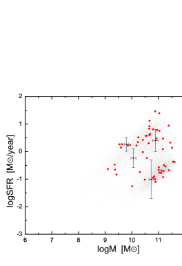
Figure 2.— Distribution of spectroscopic galaxies in the MPA/JHU catalog (grey dots), with the 53 hosted SNe (filled red circles) on a log$M$ - log$SFR$ plane. Also shown for comparison are the error bars on the masses and star formation rates of 5 randomly picked galaxies.

Figure 3.— A comparison between MPA/JHU and VESPA entries for mass (top) and SFR (bottom). Note the constant offset (dashed line), as predicted in Tojeiro et al. 2009, which is the result of a calibration offset between the VESPA and MPA databases. The scatters (standard deviation) for the masses and SFRs are 0.18 dex and 0.48 dex respectively.

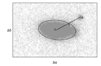
Figure 4.— Diagram illustrating the concept of $R_{25}$. The ellipse is the 25 mag/arcsec² isophote for the potential host galaxy, O is the centre, the SN Ia is at $B$, and $A$ is the point of intersection between the ellipse and line OB. $R_{25}$=OB/OA.

Figure 5.— $R_{25}$ criteria used (x-axis) plotted against number of SNe matched (y-axis). $R_{25}=3.8$, the criterion we use, is shown by the vertical line. Note that the curve flattens out very rapidly beyond this line.

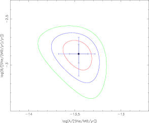
Figure 6.— Probability contours for the values of $A$ and $B$ on an $A$-$B$ plane. The red, blue and green contours represent 1$\sigma$, 2$\sigma$, 3$\sigma$ probability respectively, while the circle denotes our final maximum likelihood value. The error bars show the 1$\sigma$ and 2$\sigma$ limits of the marginalised distributions of $A$ and $B$.

Figure 7.— Specific supernova rate as a function of specific star formation rate. The black points are for our observed sample. Plotted for comparison are the predictions of our best-fit $A+B$ model (black line), the predictions of Sullivan et al. 2006 (dashed line), and their data (squares).

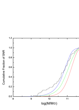
Figure 8.— Cumulative distribution functions of mass-ranked K-S tests for our best-fit $A+B$ model (green), the $A\times$M-term-only model (red), and the $B\times$SFR-term-only model (blue). The green and red lines are rejected by the K-S test, showing that our best-fit $A+B$ model and all $A+B$ models with a higher $A$/$B$ ratio do not agree with our data.

Figure 9.— Cumulative distribution functions of the specific-star-formation-ranked K-S tests for the various models. The only models which were rejected were the mass-only model (red), and the SFR-only model (blue). The remaining models ($A{\times}M+B{\times}SFR$,$A{\times}M+B{\times}SFR+C{\times}M^{-1}$,$A{\times}M+B{\times}SFR+C$, and $(A{\times}M+B{\times}SFR)(1+C{\times}M^{-1})$) all fall within the hashed blue area. As described in the text, this set of K-S tests is largely inconclusive.

Figure 10.— Cumulative distribution functions of SFR-ranked K-S tests for our best-fit $A+B$ model (green), the AM-term-only model (red), and the $B$SFR-term-only model (blue). The green and blue lines are rejected by the K-S test, showing that our best-fit $A+B$ model and all $A+B$ models with a lower $A$/$B$ ratio do not agree with our data. This, in conjunction with Fig. 8, rules out all $A+B$ models.

Figure 11.— Specific supernova rate as a function of specific star formation rate. The open points correspond to our low-mass sample, and the filled points our high-mass sample. The vertical error bars indicate Poisson uncertainties for our SNe numbers in each bin, and the horizontal error bars correspond to bin size. The trend that the open points tend to lie above the filled ones exists for all mass discrimination criteria we try. Also plotted are the predictions of our best-fit $A+B$ model. Our results have been scaled to account for observing window issues.

Figure 12.— Differential distribution functions of supernova rate as a function of host mass. The black line corresponds to our observed data, presented as number of SNe observed in each respective mass bin. The green and blue lines are the predictions of our best-fit $A+B$ model and the results of Sullivan et al. (2006) respectively. The red line is the prediction of our best-fit $A{\times}M+B{\times}SFR+C$ “constant background” model, and the cyan line corresponds to the $(A{\times}M+B{\times}SFR)(1+C{\times}M^{-1})$ model. The predictions have been scaled by the number of bins used within the plotted domain, so that the lines are comparable with those of the observed data. Our results have been scaled to account for observing window issues.

Figure 13.— Differential distribution functions of supernova rate as a function of host mass. The black line corresponds to our observed data, presented as number of SNe observed in each respective mass bin. The red and blue lines correspond to the upper and lower 1$\sigma$ limits due to the uncertainties of our results for the values of $A$ and $B$ respectively, plotted by setting both $A$ and $B$ to their upper and lower limits respectively. The green line corresponds to our best-fit values. The predictions have been scaled by the number of bins used within the plotted domain, so that the lines are comparable with those of the observed data. Our results have been scaled to account for observing window issues.

Table 1Sample of 53 Hosts for $A+B$ model fits

Host ID	$\log$M∗	$\log$SFR∗
587730847691047799	10.654	0.834
587730848501203452	9.427	-0.833
587731173306008275	11.118	-0.688
587731185114350067	11.011	-0.663
587731185668849933	11.034	-0.760
587731185669505187	10.557	0.575
587731186195366060	10.019	-1.259
587731186197332148	9.936	0.241
587731511537959123	9.590	0.147
587731511546806433	9.850	0.220
587731513142214757	10.489	-1.020
587731513142542420	10.414	-0.017
587731513143328955	10.845	-0.898
587731513146671215	11.395	-0.681
587731513679675512	10.226	0.345
587731513679610009	10.534	0.576
587731513693569205	11.017	-0.566
587731514222116993	11.444	0.326
587731514227818648	10.177	0.222
587731514231816228	11.104	-0.774
587731514232209584	11.175	0.471
587731172231872692	11.178	-0.930
587731172233183337	10.795	0.809
587731172767368214	10.664	0.919
587731174914786124	10.569	-0.229
587731185121951943	10.669	1.115
587731185126539408	9.637	0.269
587731185129554046	11.168	0.085
587731185132568670	10.878	-1.001
587731187278872773	11.386	0.940
587731512071028897	10.892	-1.102
587731512621465722	10.421	0.426
587731513427624076	9.357	-0.470
587734305949483196	11.551	-0.368
588015507661783172	9.366	-0.655
588015507672137965	10.947	0.782
588015507677642829	11.042	0.752
588015508206518484	11.207	-0.491
588015508211368141	10.247	0.518
588015508215431379	11.033	1.390
588015510339256459	11.264	-0.541
588015510339649629	11.199	-0.711
588015510363373783	10.661	0.596
588015508735393931	11.513	0.140
588015509274427469	11.608	-0.372
588015509275869191	9.540	0.263
588015509283078244	10.635	0.303
588015509285634176	10.880	1.458
588015509292319354	9.103	-0.632
588015509293760750	10.689	0.644
588015509801599099	10.790	-0.946
588015509811626061	10.926	0.479
588015509814313038	10.302	-0.744
∗ M is in M⊙, SFR is in M⊙/yr

Table 2Best-Fit Parameters from Fits and Rejection Rates of Different Models

Model	$A$	$B$	$C$	($1-\alpha_{M}$)	($1-\alpha_{sSFR}$)	($1-\alpha_{SFR}$)
	$10^{-14}(M\odot)^{-1}$	$10^{-3}(M_{\odot}$yr${}^{-1})^{-1}$	(appropriate units)
$A{\times}M+B{\times}SFR$	$3.5^{+0.9}_{-0.7}$	$1.3^{+0.4}_{-0.3}$	-	99%	97%	$<$1%
$A{\times}M+B{\times}SFR+C{\times}M^{-1}$	$3.4^{+1.0}_{-0.6}$	$1.0^{+0.4}_{-0.2}$	$2.8^{+2.2}_{-1.5}\times 10^{6}$	93%	72%	7%
$A{\times}M+B{\times}SFR+C$	$0.96^{+1.28}_{-0.95}$	$0.46^{+0.34}_{-0.26}$	$3.6^{+1.4}_{-0.4}\times 10^{-3}$	2%	34%	22%
$A{\times}M$ only	$6.8{\pm}0.9$	-	-	$>$99%	$>$99%	$>$99%
$(A{\times}M+B{\times}SFR)(1+C{\times}M^{-1})$	$1.8^{+0.7}_{-1.3}$	$0.066^{+0.046}_{-0.066}$	$3.2^{+22.0}_{-2.8}\times 10^{11}$	2%	80%	26%
$B{\times}SFR$ only	-	$2.7{\pm}0.4$	-	53%	$>$99%	$>$99%

• “$1-{\alpha}_{X}$” is the degree of rejection from a K-S test in which the galaxies are ranked by “$X$”. Passing all three tests is a necessary but insufficient condition for a model to be considered plausible.

Table 3Rejection Rates of Different Models by VESPA Data

Model	($1-\alpha_{M}$)	($1-\alpha_{SFR}$)
$A{\times}M+B{\times}SFR$	$>$99%	77%
$A{\times}M+B{\times}SFR+C{\times}M^{-1}$	$>$99%	62%
$A{\times}M+B{\times}SFR+C$	39%	42%
$A{\times}M$ only	$>$99%	$>$99%
$(A{\times}M+B{\times}SFR)(1+C{\times}M^{-1})$	34%	77%
$B{\times}SFR$ only	34%	$>$99%

References

- Abazajian et al. (2009) Abazajian, K. N., Adelman-McCarthy, J. K., Agüeros, M. A., et al. 2009, ApJS, 182, 543
- Barone-Nugent et al. (2012) Barone-Nugent, R. L., Lidman, C., Wyithe, J. S. B., et al. 2012, MNRAS, 3486
- Brinchmann et al. (2004) Brinchmann, J., Charlot, S., White, S. D. M., et al. 2004, MNRAS, 351, 1151
- Bruzual & Charlot (2003) Bruzual, G., & Charlot, S. 2003, MNRAS, 344, 1000
- Cappellari et al. (2012) Cappellari, M., McDermid, R. M., Alatalo, K., et al. 2012, Nature, 484, 485
- Charlot & Longhetti (2001) Charlot, S., & Longhetti, M. 2001, MNRAS, 323, 887
- Cooper et al. (2009) Cooper, M. C., Newman, J. A., & Yan, R. 2009, ApJ, 704, 687
- Dilday et al. (2008) Dilday, B., Kessler, R., Frieman, J. A., et al. 2008, ApJ, 682, 262
- Dilday et al. (2010) Dilday, B., Smith, M., Bassett, B., et al. 2010, ApJ, 713, 1026
- Dilday et al. (2010) Dilday, B., Bassett, B., Becker, A., et al. 2010, ApJ, 715, 1021
- Ferreras et al. (2012) Ferreras, I., La Barbera, F., de Carvalho, R. R., et al. 2012, arXiv:1206.1594
- Fioc & Rocca-Volmerange (1997) Fioc, M., & Rocca-Volmerange, B. 1997, A&A, 326, 950
- Foley (2012) Foley, R. J. 2012, ApJ, 748, 127
- Förster et al. (2006) Förster, F., Wolf, C., Podsiadlowski, P., & Han, Z. 2006, MNRAS, 368, 1893
- Frieman et al. (2008) Frieman, J. A., Bassett, B., Becker, A., et al. 2008, AJ, 135, 338
- Gallazzi et al. (2005) Gallazzi, A., Charlot, S., Brinchmann, J., White, S. D. M., & Tremonti, C. A. 2005, MNRAS, 362, 41
- Gonzalez et al. (2005) Gonzalez, A. H., Zabludoff, A. I., & Zaritsky, D. 2005, ApJ, 618, 195
- Greggio (2010) Greggio, L. 2010, MNRAS, 406, 22
- Greggio (2005) Greggio, L. 2005, A&A, 441, 1055
- Gupta et al. (2011) Gupta, R. R., D’Andrea, C. B., Sako, M., et al. 2011, ApJ, 740, 92
- Hachisu et al. (1996) Hachisu, I., Kato, M., & Nomoto, K. 1996, ApJ, 470, L97
- Han & Podsiadlowski (2006) Han, Z., & Podsiadlowski, P. 2006, MNRAS, 368, 1095
- Hillebrandt & Niemeyer (2000) Hillebrandt, W., & Niemeyer, J. C. 2000, ARA&A, 38, 191
- Kauffmann et al. (2003) Kauffmann, G., Heckman, T. M., White, S. D. M., et al. 2003, MNRAS, 341, 33
- Kelly et al. (2010) Kelly, P. L., Hicken, M., Burke, D. L., Mandel, K. S., & Kirshner, R. P. 2010, ApJ, 715, 743
- Kistler et al. (2011) Kistler, M. D., Stanek, K. Z., Kochanek, C. S., Prieto, J. L., & Thompson, T. A. 2011, arXiv:1106.3115
- Kobayashi et al. (2000) Kobayashi, C., Tsujimoto, T., & Nomoto, K. 2000, ApJ, 539, 26
- Kroupa et al. (2011) Kroupa, P., Weidner, C., Pflamm-Altenburg, J., et al. 2011, arXiv:1112.3340
- Langer et al. (2000) Langer, N., Deutschmann, A., Wellstein, S., Höflich, P. 2000, A&A, 362, 1046
- Le Borgne & Rocca-Volmerange (2002) Le Borgne, D., & Rocca-Volmerange, B. 2002, A&A, 386, 446
- Li et al. (2011) Li, W., Chornock, R., Leaman, J., et al. 2011, MNRAS, 412, 1473
- Maoz & Mannucci (2011) Maoz, D., & Mannucci, F. 2011, arXiv:1111.4492
- Maoz et al. (2012) Maoz, D., Mannucci, F., & Brandt, T.D. 2012, MNRAS, 426, 3282
- McGee & Balogh (2010) McGee, S. L., & Balogh, M. L. 2010, MNRAS, 403, L79
- Mennekens et al. (2010) Mennekens, N., Vanbeveren, D., De Greve, J. P., & De Donder, E. 2010, A&A, 515, A89
- Neill et al. (2006) Neill, J. D., Sullivan, M., Balam, D., et al. 2006, AJ, 132, 1126
- Nomoto (1982) Nomoto, K. 1982, ApJ, 253, 798
- Perlmutter et al. (1999) Perlmutter, S., Aldering, G., Goldhaber, G., et al. 1999, ApJ, 517, 565
- Perrett et al. (2012) Perrett, K., Sullivan, M., Conley, A., et al. 2012, AJ, 144, 59
- Pfahl et al. (2009) Pfahl, E., Scannapieco, E., & Bildsten, L. 2009, ApJ, 695, L111
- Pritchet et al. (2008) Pritchet, C. J., Howell, D. A., & Sullivan, M. 2008, ApJ, 683, L25
- Riess et al. (1998) Riess, A. G., Filippenko, A. V., Challis, P., et al. 1998, AJ, 116, 1009
- Sand et al. (2011) Sand, D. J., Graham, M. L., Bildfell, C., et al. 2011, ApJ, 729, 142
- Sand et al. (2012) Sand, D. J., Graham, M. L., Bildfell, C., et al. 2012, ApJ, 746, 163
- Scannapieco & Bildsten (2005) Scannapieco, E., & Bildsten, L. 2005, ApJ, 629, L85
- Schiminovich et al. (2007) Schiminovich, D., Wyder, T. K., Martin, D. C., et al. 2007, ApJS, 173, 315
- Smith et al. (2012) Smith, M., Nichol, R. C., Dilday, B., et al. 2012, ApJ, 755, 61
- Spiniello et al. (2012) Spiniello, C., Trager, S. C., Koopmans, L. V. E., & Chen, Y. P. 2012, ApJ, 753, L32
- Sullivan et al. (2006) Sullivan, M., Le Borgne, D., Pritchet, C. J., et al. 2006, ApJ, 648, 868
- Sullivan et al. (2010) Sullivan, M., Conley, A., Howell, D. A., et al. 2010, MNRAS, 406, 782
- Sullivan et al. (2011) Sullivan, M., Guy, J., Conley, A., et al. 2011, ApJ, 737, 102
- Tojeiro et al. (2009) Tojeiro, R., Wilkins, S., Heavens, A. F., Panter, B., & Jimenez, R. 2009, ApJS, 185, 1
- Totani et al. (2008) Totani, T., Morokuma, T., Oda, T., Doi, M., & Yasuda, N. 2008, PASJ, 60, 1327
- Tremonti et al. (2004) Tremonti, C. A., Heckman, T. M., Kauffmann, G., et al. 2004, ApJ, 613, 898
- Wang et al. (2010) Wang, B., Li, X.-D., & Han, Z.-W. 2010, MNRAS, 401, 2729