Wavelets in Field Theory

Abstract

We advocate the use of Daubechies wavelets as a basis for treating a variety of problems in quantum field theory. This basis has both natural large-volume and short-distance cutoffs, has natural partitions of unity, and the basis functions are all related to the fixed point of a linear renormalization group equation.

1 Introduction

Daubechies wavelets and their associated scaling functions are functions [1] [2] [3][4][5][6] that are used in signal processing and data compression. The functions have useful properties that have advantages for applications to problems in quantum field theory. Daubechies wavelets have been used in some field-theoretic applications [7] [8] [9] [10] and different types of wavelets have been used in more formal treatments of field theory [11] [12] [13] [14] [15] however many useful properties of wavelets do not appear to have been exploited. Some of the properties of Daubechies wavelets that are potentially useful for field theory applications are:

• The functions are an orthonormal basis for the square integrable functions on the line. This means that one can formally express fields exactly as infinite linear combinations of discrete field operators and coefficient functions. This can be used to study the nature of corrections to truncated theories or to compute the singular coefficients in operator product expansions.

• The basis functions have compact support. This means that discrete fields associated with basis functions with space-like separated support commute. The maximum size of the support of the basis functions can be controlled. There are also infinite numbers of basis functions with arbitrarily small support so it is possible to use these operators study locality and how locality is violated in truncations. In these representations local fields can be replaced by a local algebra of well-defined operators.

• The Daubechies basis functions are related to solutions of a linear renormalization group equation. It is a natural basis to formulate renormalization group transformations. The basis allows for a separation of scales; a fine resolution truncated Lagrangian or Hamiltonian can be exactly expressed in terms of a coarse resolution truncated Lagrangian or Hamiltonian of the same form, plus some addition operators that fill in the missing fine-scale physics. Eliminating the fine-scale operators gives a new Hamiltonian, involving the same masses and coupling constants, in the coarse-scale degrees of freedom that includes the effects of the eliminated fine-scale degree of freedom. This can be repeated to include the effects of eliminated degrees of freedom on arbitrarily small scales.

• The basis is generated from a single function, which is the solution of the linear renormalization group equation, using discrete unitary translations and discrete unitary scale transformations. While the basis functions have a fractal structure, overlap integrals of products of any number of the basis functions and low-order derivatives can be computed analytically using only the renormalization group equation and a scale fixing condition. In addition, integrals of products of basis functions and polynomials can also be computed exactly using the renormalization group equations.

• Subsets of the basis functions contain compact, locally-finite partitions of unity. This property can be used to investigate symmetries like Poincaré invariance. The partitions of unity can be used to make local realizations of the Lie algebra. The generators can be expressed exactly as sums of localized operators obtained by integrating the operator densities multiplied by the functions in the partition of unity.

• The basis functions have a limited amount of smoothness, and can locally pointwise represent low-degree polynomials. This means that overlaps of low-order derivatives of field operators can be computed directly, rather than by using a finite-difference approximation.

• Because the basis functions have compact support and there are basis functions with arbitrarily small support, the basis has both natural short-distance and large-volume cutoffs.

The purpose of this paper is to discuss some problems in field theory where wavelets might have advantages as well as some of the specialized methods for dealing with fractal basis functions. In section two we discuss the construction of the wavelet basis and introduce the renormalization group equation for the Daubechies scaling function. In section three we introduce our free-field conventions. In section four we introduce the wavelet representation of free fields. This representation is also relevant in interacting theories, when the natural volume and resolution truncations in the wavelet representation are used to make finite number of degree-of-freedom truncations of the interacting theory. In section five we discuss the scaling properties of the wavelet fields. In section six we discuss Poincaré invariance and partitions of unity. In section seven we discuss the formulation of renormalization group equations in the wavelet basis. In section eight we discuss gauge transformations in the wavelet representation. In the appendix we compute the overlap coefficients that couple different scales in the free-field Hamiltonian.

2 Basis construction

The Daubechies scaling function is the solution of a linear renormalization group equation subject to a scale-fixing normalization condition. All basis functions are generated from the scaling function using discrete translations, dyadic scale transformations, and sums.

The discrete translation operator, $T$, and the dyadic scale transformation, $D$, are unitary operators on $L^{2}(\mathbb{R})$ defined by

$$(Df)(x)=\sqrt{2}f(2x)\qquad(Tf)(x)=f(x-1).$$ (1)

The operator $D$ decreases the support of a function with compact support by a factor of two in a manner that preserves the $L^{2}(\mathbb{R})$ norm. The scaling function, $s(x)$, is the solution of the linear renormalization group equation,

$$s(x)=\sum_{n=0}^{2K-1}h_{n}DT^{n}s(x),$$ (2)

called the scaling equation. Equation (2) states that the scaling function is a linear combination of $2K$-translated copies of itself on a scale smaller by a factor of 2. Since this is a homogeneous equation for $s(x)$, we are free to assign the normalization. It is fixed by the scale-fixing condition

$$\int s(x)dx=1.$$ (3)

Equations (2-3) define the scaling function. The $h_{n}$ are real coefficients that are characteristic of the type of wavelet. The coefficients for some of the Daubechies scaling functions are given in Table 1.

Given the solution of (2-3), scale-$1/2^{k}$ scaling functions are defined by applying $n$ unit translations followed by $k$ dyadic scale transformations to the original scaling function,

$$s_{n}^{k}(x):=D^{k}T^{n}s(x).$$ (4)

Linear combinations of these functions with square-sumable coefficients span a subspace ${\cal H}_{k}$ of $L^{2}(\mathbb{R})$, which we call the resolution-$1/2^{k}$ subspace. The scaling equation implies the relation

$${\cal H}_{k+1}\supset{\cal H}_{k}$$ (5)

and more generally

$${\cal H}_{k+m}\supset{\cal H}_{k}$$ (6)

for $m>0$. This means that the lower-resolution spaces are linear subspaces of the higher-resolution spaces.

The mother wavelet, $w(x)$, is defined as the following linear combination of the $s_{n}^{1}(x)$ scaling functions:

$$w(x)=\sum_{n=0}^{2K-1}g_{n}DT^{n}s(x)=\sum_{n=0}^{2K-1}g_{n}s^{1}_{n}(x)$$ (7)

where the coefficients $g_{n}$ are related to the coefficients $h_{n}$ by reversing the order and alternating the signs

$$g_{n}=(-)^{n}h_{2K-1-n}.$$ (8)

Plots of the Daubechies $K=3$ scaling function and mother wavelet are given in figures 1 and 2.

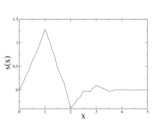
Figure 1: Daubechies $K=3$ scaling function.

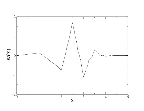
Figure 2: Daubechies $K=3$ mother wavelet

Scale-$1/2^{k}$ wavelets, $w_{n}^{k}(x)$, are constructed by applying translations and dyadic scale transformations to the mother wavelet

$$w_{n}^{k}(x)=D^{k}T^{n}w(x).$$ (9)

The scale $1/2^{k}$ wavelets are designed to span the orthogonal complement, ${\cal W}_{k}$, of ${\cal H}_{k}$ in ${\cal H}_{k+1}$,

$${\cal H}_{k+1}={\cal H}_{k}\oplus{\cal W}_{k}.$$ (10)

The coefficients $h_{l}$ are chosen so the translates of the scaling function and mother wavelet are orthonormal and finite linear combinations of translations of the scaling function can be used to make local pointwise representations of polynomials of degree $K-1$.

Continuing the decomposition (10) inductively leads to the following orthogonal direct sum decomposition of the Hilbert space of square integrable functions on the line

$$L^{2}(\mathbb{R})={\cal H}_{k}\oplus{\cal W}_{k}\oplus{\cal W}_{k+1}\oplus\cdots.$$ (11)

This gives a decomposition of the Hilbert space into orthogonal subspaces with successively finer resolutions. Specifically, the basis for ${\cal H}_{k}$ can be used to represent features down to scale $1/2^{k}$, ${\cal W}_{k}$ represents features down to scale $1/2^{k+1}$ that cannot be represented on scale $1/2^{k}$, ${\cal W}_{k+1}$ represents features down to scale $1/2^{k+2}$ that cannot be represented on scale $1/2^{k+1}$, etc.. Smearing local fields with these basis functions gives discrete fields that are sensitive to average information on different scales.

The coefficients $h_{n}$, which characterize the Daubechies $K$-wavelets, are solutions of the system of equations

$$\sum_{n=0}^{2K-1}h_{n}=\sqrt{2}$$ (12)

$$\sum_{n=0}^{2K-1}h_{n}h_{n-2m}=\delta_{m0}$$ (13)

$$\sum_{n=0}^{2K-1}n^{m}g_{n}=\sum_{n=0}^{2K-1}n^{m}(-1)^{n}h_{2K-1-n}=0\qquad m<K.$$ (14)

The first equation is a necessary condition for the scaling equation to have a solution; it can be derived by taking the Fourier transform of both sides of the scaling equation. The second equation ensures that integer translates of the scaling function are orthonormal. The third equation ensures that linear combinations of integer translates of the wavelet functions are orthogonal to degree $K-1$ polynomials.

This last condition, along with (11), implies that polynomials of degree $K-1$ can be locally pointwise represented by locally finite linear combinations of scaling functions.

The solution of these equations for $K=1,2,3$ are given in Table 1. The solutions are unique up to reversal of order; $n\to 2K-1-n$.

$h_{n}$	K=1	K=2	K=3
$h_{0}$	$1/\sqrt{2}$	$(1+\sqrt{3})/4\sqrt{2}$	$(1+\sqrt{10}+\sqrt{5+2\sqrt{10}})/16\sqrt{2}$
$h_{1}$	$1/\sqrt{2}$	$(3+\sqrt{3})/4\sqrt{2}$	$(5+\sqrt{10}+3\sqrt{5+2\sqrt{10}})/16\sqrt{2}$
$h_{2}$	$0$	$(3-\sqrt{3})/4\sqrt{2}$	$(10-2\sqrt{10}+2\sqrt{5+2\sqrt{10}})/16\sqrt{2}$
$h_{3}$	$0$	$(1-\sqrt{3})/4\sqrt{2}$	$(10-2\sqrt{10}-2\sqrt{5+2\sqrt{10}})/16\sqrt{2}$
$h_{4}$	$0$	$0$	$(5+\sqrt{10}-3\sqrt{5+2\sqrt{10}})/16\sqrt{2}$
$h_{5}$	$0$	$0$	$(1+\sqrt{10}-\sqrt{5+2\sqrt{10}})/16\sqrt{2}$

Table 1:

The numerical values of the $K=3$ coefficients, rounded to two decimal places, are $h_{0}=-g_{5}=.43$, $h_{1}=g_{4}=1.11$, $h_{2}=-g_{3}=.66$, $h_{3}=g_{2}=-.34$, $h_{4}=-g_{1}=-.39$, $h_{5}=g_{0}=-.66$. An important observation is that only one of the six coefficients, $h_{1}=g_{4}$ has magnitude larger than $1$.

In this work we advocate using the Daubechies $K=3$ wavelets. This is because they have small support and have one continuous derivative. The derivative allows one to replace the finite-difference approximations of derivatives that appear in the Hamiltonian or Lagrangian densities with actual derivatives.

The scaling function $s(x)$ and mother wavelet $w(x)$ have support on the interval $[0,2K-1]$. It follows from (11) that for any fixed scale, $1/2^{k}$, the functions

$$\{s^{k}_{n}(x)\}_{n=-\infty}^{\infty}\cup\{w^{m}_{n}(x)\}_{n=-\infty,m=k}^{\infty,\infty}$$ (15)

are an orthonormal basis for $L^{2}(\mathbb{R})$. The basis functions $s^{k}_{n}(x)$ and $w^{k}_{n}(x)$ have compact support on the interval $[2^{-k}n,2^{-k}(n+2K-1)]$. This support justifies calling ${\cal H}_{k}$ the resolution-$1/2^{k}$ subspace.

The basis functions satisfy the orthonormality conditions

$$\int dxs^{k}_{n}(x)s^{k}_{m}(x)=\delta_{mn}$$ (16)

$$\int dxs^{k}_{n}(x)w^{k+l}_{m}(x)=0\qquad(l\geq 0)$$ (17)

$$\int dxw^{k}_{n}(x)w^{l}_{m}(x)=\delta_{mn}\delta_{kl}.$$ (18)

Scaling functions with different $k$ are not orthogonal and are not members of the same basis. Similarly, the $w^{k+l}_{m}(x)$ with negative $l$ are not orthogonal to $s^{k}_{m}(x)$ and are not members of the basis that includes the $s^{k}_{m}(x)$. In general, the basis (15) consists of scaling functions, $s_{m}^{k}(x)$, of a fixed largest scale, $1/2^{k}$, and wavelets, $w^{k+l}_{m}(x)$, that can represent the structure on all scales, $1/2^{k+l}$, with $l\geq 0$.

A basis for the resolution $1/2^{k+m}$ subspace, ${\cal H}_{k+m}$, that includes the basis functions for the resolution $1/2^{k}$ subspace, ${\cal H}_{k}$, is

$$\mbox{span}(\{s^{k+m}_{n}\}_{n=-\infty}^{\infty})=\mbox{span}(\{s^{k}_{n}\}_{n=-\infty}^{\infty}\cup\{w^{l}_{n}\}_{n=-\infty,l=k}^{\infty,k+m-1}).$$ (19)

This means that the wavelets on scales $1/2^{k},1/2^{k+1},\cdots,1/2^{k+m-1}$ fill in all of the missing finer-resolution information in ${\cal H}_{k+m}$ that is not contained in ${\cal H}_{k}$.

The scaling functions form a partition of unity

$$1=\sum_{n=-\infty}^{\infty}s(x-n)=\sum_{n=-\infty}^{\infty}(T^{n}s)(x)=\sum_{n=-\infty}^{\infty}s_{n}^{0}(x).$$ (20)

This partition of unity is locally finite, meaning that at any point only a finite number of the functions are non-zero, and the functions all have compact support. There are also partitions of unity for the scale-$1/2^{k}$ scaling functions

$$\sum_{n=-\infty}^{\infty}{1\over\sqrt{2^{k}}}s^{k}_{n}(x)=\sum_{n=-\infty}^{\infty}s(2^{k}x-n)=1$$ (21)

except they must be multiplied by the factor ${1\over\sqrt{2^{k}}}$.

The scale-$1/2^{k-1}$ scaling functions and scale-$1/2^{k-1}$ wavelets are both linear combinations of the scale $1/2^{k}$ scaling functions

$$s^{k-1}_{n}(x)=\sum_{l=0}^{2K-1}h_{l}s^{k}_{2n+l}(x)$$ (22)

$$w^{k-1}_{n}(x)=\sum_{l=0}^{2K-1}g_{l}s^{k}_{2n+l}(x).$$ (23)

The inverse of these relations express the scale $1/2^{k}$ scaling function as a linear combination of the scale $1/2^{k-1}$ scaling functions and wavelets

$$s^{k}_{n}(x)=\sum_{m}h_{n-2m}s^{k-1}_{m}(x)+\sum_{m}g_{n-2m}w^{k-1}_{m}(x).$$ (24)

Equations (22-23) define the wavelet transform in signal processing. It is a pair of filters that decompose a signal into high and low-resolution parts in a manner that can be inverted to reconstruct the full signal. In signal processing applications it is applied many times to generate a multi-resolution decomposition of the signal. Equation (24) is relevant in field-theory applications, where we see that the wavelets represent the lost information when one discards small-scale degrees of freedom. The same coefficients appear in (22-23) and (24) because these two sets of orthonormal basis functions on ${\cal H}^{k}$ are related by a real orthogonal transformation.

For some applications it is useful to express equations (22) and (23) in infinite matrix form

$$s^{k-1}_{n}(x)=\sum_{m=2n}^{2n+2K-1}H_{nm}s^{k}_{m}(x)$$ (25)

$$w^{k-1}_{n}(x)=\sum_{m=2n}^{2n+2K-1}G_{nm}s^{k}_{m}(x)$$ (26)

where

$$H_{nm}=h_{m-2n}\qquad G_{nm}=g_{m-2n}.$$ (27)

In this notation (24) becomes

$$s^{k}_{n}(x)=\sum_{m}{H}^{t}_{nm}s^{k-1}_{m}(x)+\sum_{m}{G}^{t}_{nm}w^{k-1}_{m}(x)$$ (28)

where

$${H}^{t}_{nm}=H_{mn}=h_{n-2m}\qquad{G}^{t}_{nm}=G_{mn}=g_{n-2m}.$$ (29)

While the matrices are in principle infinite, for fixed $n$ there are only $2K$ non-vanishing terms in the sum, which is clear in the equivalent expressions (22) and (23).

Note that if we set $x=n$ in the scaling equation it becomes

$$s(n)=\sum_{l=0}^{2K-1}\sqrt{2}h_{l}s(2n-l)=\sqrt{2}\sum_{m=2n-2K+1}^{2n}h_{2n-m}s(m)$$ (30)

which has the form of an eigenvalue equation for the matrix, $M_{nm}=h_{2n-m}$, where the eigenvectors are $(0,s(1),s(2),\cdots,s(2K-2),0)$ and the eigenvalue is $1/\sqrt{2}$. If we differentiate the scaling equation and again evaluate the derivative of the scaling functions at integer values we get

$$s^{\prime}(n)=\sum_{l=0}^{2K-1}2\sqrt{2}h_{l}s^{\prime}(2n-l)=2\sqrt{2}\sum_{m=2n-2K+1}^{2n}h_{2n-m}s^{\prime}(m).$$ (31)

This is an eigenvalue equation for the same matrix, with eigenvector $(s^{\prime}(0),s^{\prime}(1)$, $s^{\prime}(2),\cdots,s^{\prime}(2K-2),s^{\prime}(2K-1))$ and eigenvalue $1/2^{3/2}$. Each derivative brings down an additional factor of 1/2 in the eigenvalue. Since a finite matrix has a finite number of eigenvalues, the scaling function can only be differentiated a finite number of times, ($n$ times if the matrix above has an eigenvalues of $2^{-(n+1/2)}$). Thus we have the interesting property that the number of derivatives is associated with the eigenvalue spectrum of a finite-dimensional matrix. This makes it clear that the individual wavelets and scaling functions have only a finite number of derivatives. It is interesting that certain linear combinations of scaling functions may have more derivatives than the functions themselves; this is the case with the partition of unity (20). The sum is constant, which is infinitely differentiable, but the individual functions in the sum are not!

For fields that are functions of four space-time variables, we use a basis for the square integrable functions of the three space variables consisting of products of the wavelet basis functions, (15), in each of the three variables. We identify basis functions that are the product of three resolution $1/2^{k}$ scaling functions as the resolution $1/2^{k}$ basis; the seven other products of combinations of wavelets and scaling functions span the orthogonal complement of the resolution $1/2^{k}$ subspace in $L^{2}(\mathbb{R}^{3})$. We introduce a compact notation to make the three-dimensional case look like the one-dimensional case.

In three dimensions we define:

$$s_{\mathbf{n}}^{k}(\mathbf{x})=s^{k}_{n_{1}}(x_{1})s^{k}_{n_{2}}(x_{2})s^{k}_{n_{3}}(x_{3})$$ (32)

and use the notation to $w_{\mathbf{n},\alpha}^{m}(\mathbf{x})$ to represent the remaining basis functions that have one of the following seven forms

$$w_{\mathbf{n},1,k_{3}}^{m}(\mathbf{x}):=s^{k}_{n_{1}}(x_{1})s^{k}_{n_{2}}(x_{2})w^{k_{3}}_{n_{3}}(x_{3})$$ (33)

$$w_{\mathbf{n},2,k_{2}}^{m}(\mathbf{x}):=s^{k}_{n_{1}}(x_{1})w^{k_{2}}_{n_{2}}(x_{2})s^{k}_{n_{3}}(x_{3})$$ (34)

$$w_{\mathbf{n},3,k_{1}}^{m}(\mathbf{x}):=w^{k_{1}}_{n_{1}}(x_{1})s^{k}_{n_{2}}(x_{2})s^{k}_{n_{3}}(x_{3})$$ (35)

$$w_{\mathbf{n},4,k_{2},k_{3}}^{m}(\mathbf{x}):=s^{k}_{n_{1}}(x_{1})w^{k2}_{n_{2}}(x_{2})w^{k3}_{n_{3}}(x_{3})$$ (36)

$$w_{\mathbf{n},5,k_{1},k_{2}}^{m}(\mathbf{x}):=w^{k_{1}}_{n_{1}}(x_{1})w^{k_{2}}_{n_{2}}(x_{2})s^{k}_{n_{3}}(x_{3})$$ (37)

$$w_{\mathbf{n},6,k_{1},k_{3}}^{m}(\mathbf{x}):=w^{k_{1}}_{n_{1}}(x_{1})s^{k}_{n_{2}}(x_{2})w^{k_{3}}{n_{3}}(x_{3})$$ (38)

$$w_{\mathbf{n},7,k_{1},k_{2},k_{3}}^{m}(\mathbf{x}):=w^{k_{1}}_{n_{1}}(x_{1})w^{k_{2}}_{n_{2}}(x_{2})w^{k_{3}}_{n_{3}}(x_{3}).$$ (39)

We call the functions $w_{\mathbf{n},\alpha}^{m}(\mathbf{x})$ generalized wavelets, where the index, $m$, represents the smallest wavelet scale (largest $k_{1},k_{2},k_{3}$) appearing in the product. The index $\alpha$ indicates the values of $k_{1},k_{2},k_{3}$ as well as which of the seven types of products appear in the basis function.

Since the scaling function is the solution of a renormalization group equation and all of the other basis functions are linear combinations of translated and scale-transformed scaling functions, it follows that all of the basis functions have a fractal structure. This makes it difficult to represent the basis functions in terms of elementary functions that are smooth on a sufficiently small scale. Fortunately, while it is possible to compute the scaling function to any desired accuracy, this is never needed in any application. What is needed are the overlap integrals of products of arbitrary numbers of basis functions and their derivatives. It turns out that these integrals satisfy renormalization group equations and can all be computed exactly using the renormalization group equations and the normalization condition, without knowing the value of the integrand at any points. These equations can also be used to compute the integrals of products of these functions with polynomials of arbitrary degree. Since the basis functions have compact support, and any continuous function can be approximated by a polynomial on a compact interval, it follows that integrals of products of these basis functions and continuous functions can be computed to any desired accuracy. Methods for computing these quantities are discussed in section five and the appendix.

3 Free field conventions

In this section we summarize our conventions for a free mass-$\mu$ scalar field and list some standard results that will be used in the subsequent sections. Since the free field operators exist and the wavelet basis expansions are exact, free fields provide a useful laboratory for understanding truncations as approximations.

Free fields also play a role in modeling interacting theories. In the presence of both resolution and volume cutoffs, which are natural in the wavelet basis, all of the operator products in the Hamiltonain become finite sums of well-defined operators on the free-field Fock space, allowing one to formally work in the interaction representation. The renormalization group, discussed in section seven, provides one means to investigate the existence of a limiting interacting theory with an infinite number of degrees of freedom.

The Lagrangian density for a free scalar field of mass $\mu$ is

$${\cal L}(x):={1\over 2}(\dot{\Phi}(x)\dot{\Phi}(x)-\boldsymbol{\nabla}\Phi(x)\cdot\boldsymbol{\nabla}\Phi(x)-\mu^{2}\Phi(x)^{2}).$$ (40)

Lagrange’s equations are

$${\partial^{2}\over\partial t^{2}}\Phi(x)-{\partial^{2}\over\partial\mathbf{x}^{2}}\Phi(x)+\mu^{2}\Phi(x)=0.$$ (41)

The generalized momentum is

$$\Pi(x)={\partial{\cal L}(x)\over\partial\dot{\Phi}}=\dot{\Phi}(x)$$ (42)

and the Hamiltonian is

$$H=\int(\Pi(x)\dot{\Phi}(x)-{\cal L}(x))d\mathbf{x}$$

$$={1\over 2}\int({\Pi}(x){\Pi}(x)+\boldsymbol{\nabla}\Phi(x)\cdot\boldsymbol{\nabla}\Phi(x)+\mu^{2}\Phi(x)^{2})d\mathbf{x}.$$ (43)

The field $\Phi(\mathbf{x},t)$ is normalized so $\Phi(\mathbf{x},t)$ and $\Pi(\mathbf{x},t)$ satisfy the canonical equal-time commutation relations

$$[\Phi(\mathbf{x},t),\Pi(\mathbf{y},t)]=i\delta(\mathbf{x}-\mathbf{y}).$$ (44)

The classical energy-momentum tensor is

$$T^{\mu\nu}(x)=-{\partial{\cal L}(x)\over\partial(\partial_{\mu}\Phi)}\partial^{\nu}\Phi+\eta^{\mu\nu}{\cal L}(x)=$$

$$\partial^{\mu}\Phi(x)\partial^{\nu}\Phi(x)-{1\over 2}\eta^{\mu\nu}(\partial^{\alpha}\Phi(x)\partial_{\alpha}\Phi(x)+\mu^{2}\Phi(x)^{2})$$ (45)

and the angular momentum tensor is

$$M^{\mu\nu\alpha}=(x^{\mu}T^{\nu\alpha}-x^{\nu}T^{\mu\alpha}).$$ (46)

These tensors satisfy the conservation laws

$$\partial_{\mu}T^{\nu\mu}=\partial_{\alpha}M^{\mu\nu\alpha}=0$$ (47)

leading to the conserved charges, which after quantization, are the infinitesimal generators of the Poincaré group

$$P^{\mu}=\int_{t=0}d\mathbf{x}{\cal P}^{\mu}(x)d\mathbf{x}\qquad{\cal P}^{\mu}(x):=T^{\mu 0}(x)$$ (48)

$$J^{\mu\nu}:=\int_{t=0}d\mathbf{x}{\cal J}^{\mu\nu}(x)d\mathbf{x}\qquad{\cal J}^{\mu\nu}(x):=M^{\mu\nu 0}(x).$$ (49)

The generators can be expressed as integrals over operator-valued densities

$$H=P^{0}=$$

$$\int_{t=0}:(\Pi(x)\dot{\Phi}(x)-{\cal L}(x)):d\mathbf{x}={1\over 2}\int:({\Pi}(x){\Pi}(x)+\boldsymbol{\nabla}\Phi(x)\cdot\boldsymbol{\nabla}\Phi(x)+\mu^{2}\Phi(x)^{2}):d\mathbf{x}$$ (50)

$$\mathbf{P}=-\int_{t=0}:\Pi(x)\boldsymbol{\nabla}\Phi(x):d\mathbf{x}$$ (51)

$$J^{ij}=-J^{ji}=\epsilon^{ijk}J^{k}=$$

$$\int_{t=0}d\mathbf{x}:(\Pi(x)x^{j}\partial^{i}\Phi(x)-\Pi(x)x^{i}\partial^{j}\Phi(x)):$$ (52)

$$J^{i0}=-J^{0i}=K^{i}=$$

$$\int_{t=0}:\left({1\over 2}\Pi^{2}(x)x^{i}+{1\over 2}x^{i}\boldsymbol{\nabla}\Phi(x)\cdot\boldsymbol{\nabla}\Phi(x)+{1\over 2}x^{i}\mu^{2}\Phi(x)^{2}\right):d\mathbf{x}$$ (53)

where the $:$s indicate that the operators are normal ordered.

The field has the Fourier representation ($-+++$ metric)

$$\Phi(x)={1\over(2\pi)^{3/2}}\int{d\mathbf{p}\over\sqrt{2\omega_{\mu}(\mathbf{p})}}(e^{-ip\cdot x}a^{\dagger}(\mathbf{p})+e^{ip\cdot x}a(\mathbf{p}))$$ (54)

$$\Pi(x)={i\over(2\pi)^{3/2}}\int d\mathbf{p}\sqrt{{\omega_{\mu}(\mathbf{p})\over 2}}(e^{-ip\cdot x}a^{\dagger}(\mathbf{p})-e^{ip\cdot x}a(\mathbf{p}))$$ (55)

where

$$\omega_{\mu}(\mathbf{p})=\sqrt{\mu^{2}+\mathbf{p}^{2}}$$ (56)

is the single-particle energy. The equal-time commutation relations imply

$$[a(\mathbf{p}),a^{\dagger}(\mathbf{p}^{\prime})]=\delta(\mathbf{p}-\mathbf{p}^{\prime}).$$ (57)

The vacuum state of the field is the solution of

$$a(\mathbf{p})|0\rangle=0.$$ (58)

The infinitesimal generators have momentum-space representations as integrals over momentum densities

$$H=\int{\cal H}(\mathbf{p})d\mathbf{p}=\int d\mathbf{p}a^{\dagger}(\mathbf{p})\omega_{m}(\mathbf{p})a(\mathbf{p}),$$ (59)

$$\mathbf{P}=\int\boldsymbol{{\cal P}}(\mathbf{p})d\mathbf{p}=\int d\mathbf{p}a^{\dagger}(\mathbf{p})\mathbf{p}a(\mathbf{p}),$$ (60)

$$\mathbf{J}=\int\boldsymbol{{\cal J}}(\mathbf{p})d\mathbf{p}=\int d\mathbf{p}a^{\dagger}(\mathbf{p})(i{\partial\over\partial\mathbf{p}}\times\mathbf{p})a(\mathbf{p}),$$ (61)

$$\mathbf{K}=\int\boldsymbol{{\cal K}}(\mathbf{p})d\mathbf{p}=\int d\mathbf{p}a^{\dagger}(\mathbf{p}){1\over 2}\{i{\partial\over\partial\mathbf{p}},\omega_{m}(\mathbf{p})\}a(\mathbf{p})$$ (62)

where we set $x^{0}=0$ in the last expression.

4 Wavelet discretized fields

The wavelet basis discussed in (32-39) can be used to write exact expansions of the fields as sums of products of basis functions with time-dependent operator coefficients,

$$\Phi(\mathbf{x},t)=\sum_{\mathbf{n}}\Phi^{k}(\mathbf{n},t)s_{\mathbf{n}}^{k}(\mathbf{x})+\sum_{\mathbf{n},\alpha,l\geq k}\Phi^{l}(\mathbf{n},\alpha,t)w^{l}_{\mathbf{n}\alpha}(\mathbf{x})$$ (63)

$$\Pi(\mathbf{x},t)=\sum_{\mathbf{n}}\Pi^{k}(\mathbf{n},t)s_{\mathbf{n}}^{k}(\mathbf{x})+\sum_{\mathbf{n},\alpha,l\geq k}\Pi^{l}(\mathbf{n},\alpha,t)w^{l}_{\mathbf{n}\alpha}(\mathbf{x}),$$ (64)

where the operator coefficients are projections of the field operators on the orthonormal basis of scaling functions and wavelets

$$\Phi^{k}(\mathbf{n},t)=\int d\mathbf{x}\Phi(\mathbf{x},t)s_{\mathbf{n}}^{k}(\mathbf{x})$$ (65)

$$\Phi^{l}(\mathbf{n},\alpha,t)=\int d\mathbf{x}\Phi(\mathbf{x},t)w^{l}_{\mathbf{n}\alpha}(\mathbf{x})\qquad(l\geq k)$$ (66)

$$\Pi^{k}(\mathbf{n},t)=\int d\mathbf{x}\Pi(\mathbf{x},t)s_{\mathbf{n}}^{k}(\mathbf{x})$$ (67)

$$\Pi^{l}(\mathbf{n},\alpha,t)=\int d\mathbf{x}\Pi(\mathbf{x},t)w^{l}_{\mathbf{n}\alpha}(\mathbf{x})\qquad(l\geq k).$$ (68)

In these expressions the spacetime points have dimensions. If $L$ is a length scale then replacing $s^{k}_{m}(x)$ and $w^{l}_{n}(x)$ by ${1\over\sqrt{L}}s^{k}_{m}({x\over L})$ and ${1\over\sqrt{L}}w^{l}_{n}({x\over L})$ preserves all of the formulas in the previous section, except the translations and rescaling are in units of $L$. The scale factors $1/2^{k}$ remain dimensionless. All factors of $L$ disappear if we make this change and use natural units where $L=1$.

In these expression we only integrate over the spatial coordinates $\mathbf{x}$ so the operator coefficients are time dependent. It is also possible to integrate over all space-time coordinates, which is useful in action-based formulations.

These expansions have been separated into operators smeared over scaling functions and generalized wavelets. This is a separation of scales - the scale-$1/2^{k}$ scaling functions give the coarse-scale structure of the field, while the wavelet parts include the structure on all smaller scales.

The field operators smeared with the scaling functions represent the average value of the field over a compact region weighted by the product of scaling functions. Because the scale $1/2^{k+1}$ scaling function can be expressed in terms of the scale $1/2^{k}$ scaling functions and scale $1/2^{k}$ wavelets, (24), the scale $1/2^{k}$ wavelet and scaling-function smeared fields, contain the same information as the scale $1/2^{k+1}$ scaling-function smeared fields.

When all of the wavelet contributions are included the expansions are exact. In any finite region there are still an infinite number of wavelet basis functions associated with arbitrarily small scales.

For fields satisfying canonical equal-time commutation relations, the orthonormality of the basis functions implies that the equal-time canonical commutation relations for the discrete fields are:

$$[\Phi^{k}(\mathbf{n},t),\Phi^{k}(\mathbf{m},t)]=0\qquad[\Pi^{k}(\mathbf{n},t),\Pi^{k}(\mathbf{m},t)]=0$$ (69)

$$[\Phi^{k}(\mathbf{n},t),\Pi^{k}(\mathbf{m},t)]=i\delta_{\mathbf{n},\mathbf{m}}$$ (70)

$$[\Phi^{r}(\mathbf{n},\alpha,t),\Phi^{s}(\mathbf{m},\beta,t)]=0\qquad[\Pi^{r}(\mathbf{n},\alpha,t),\Pi^{s}(\mathbf{m},\beta,t)]=0$$ (71)

$$[\Phi^{r}(\mathbf{n},\alpha,t),\Pi^{s}(\mathbf{m},\beta,t)]=i\delta_{\alpha\beta}\delta_{rs}\delta_{\mathbf{n},\mathbf{m}}$$ (72)

$$[\Phi^{r}(\mathbf{n},\alpha,t),\Phi^{s}(\mathbf{m},t)]=0\qquad[\Pi^{r}(\mathbf{n},\alpha,t),\Pi^{s}(\mathbf{m},t)]=0$$ (73)

$$[\Phi^{r}(\mathbf{n},\alpha,t),\Pi^{s}(\mathbf{m},t)]=0\qquad[\Pi^{r}(\mathbf{n},\alpha,t),\Phi^{s}(\mathbf{m},t)]=0$$ (74)

where in all of these expressions $k\leq r,s$.

Given these discrete field operators we can construct discrete creation and annihilation operators

$$a^{k}(\mathbf{n},t):={1\over\sqrt{2}}(\sqrt{\gamma}\Phi^{k}(\mathbf{n},t)+i{1\over\sqrt{\gamma}}\Pi^{k}(\mathbf{n},t))$$ (75)

$$b^{r}(\mathbf{n},\alpha,t):={1\over\sqrt{2}}((\sqrt{\gamma}\Phi^{k}(\mathbf{n},\alpha,t)+i{1\over\sqrt{\gamma}}\Pi^{k}(\mathbf{n},\alpha,t))$$ (76)

that satisfy

$$[a^{k}(\mathbf{n},t),a^{k\dagger}(\mathbf{m},t)]=\delta_{\mathbf{m}\mathbf{n}}$$ (77)

$$[b^{l}(\mathbf{n},\alpha,t),b^{j\dagger}(\mathbf{m},\beta,t)]=\delta_{\mathbf{m}\mathbf{n}}\delta_{jl}\delta_{\alpha\beta}$$ (78)

with all other commutators vanishing. In these expressions $\gamma$ is a constant that can depend on the discrete indices. While these quantities and their adjoints satisfy the commutation relations (77,78) for creation and annihilation operators for any choice of $\gamma$, a specific choice is required if the annihilation operator is to annihilate the free field vacuum. This requires that $\gamma$ is chosen so

$$\langle 0|a^{k\dagger}(\mathbf{n},t)a^{k}(\mathbf{n},t)|0\rangle=0$$ (79)

$$\langle 0|b^{r\dagger}(\mathbf{n},\alpha,t)b^{r}(\mathbf{n},\alpha,t)|0\rangle=0$$ (80)

$$\langle 0|a^{k}(\mathbf{n},t)a^{k\dagger}(\mathbf{n},t)|0\rangle=1$$ (81)

$$\langle 0|b^{r}(\mathbf{n},\alpha,t)b^{r\dagger}(\mathbf{n},\alpha,t)|0\rangle=1$$ (82)

which leads to quadratic equations for the coefficients $\gamma$. With this choice of $\gamma$ the annihilation operators annihilate the mass $\mu$ free-field vacuum.

The solution of these equations for the scaling-function fields is

$$\gamma(k)={1\pm\sqrt{1-4\langle 0|\Phi^{k}(\mathbf{m},t)\Phi^{k}(\mathbf{m},t)|0\rangle\langle 0|\Pi^{k}(\mathbf{m},t)\Pi^{k}(\mathbf{m},t)|0\rangle}\over 2\langle 0|\Phi^{k}(\mathbf{m},t)\Phi^{k}(\mathbf{m},t)|0\rangle}$$

$$={1\pm\sqrt{1-4\langle 0|\Phi^{k}(\mathbf{0},0)\Phi^{k}(\mathbf{0},0)|0\rangle\langle 0|\Pi^{k}(\mathbf{0},0)\Pi^{k}(\mathbf{0},0)|0\rangle}\over 2\langle 0|\Phi^{k}(\mathbf{0},0)\Phi^{k}(\mathbf{0},0)|0\rangle}$$ (83)

and for the wavelet fields

$$\gamma(k,\alpha)={1\pm\sqrt{1-4\langle 0|\Phi^{r}(\mathbf{m},\alpha,t)\Phi^{r}(\mathbf{m},\alpha,t)|0\rangle\langle 0|\Pi^{r}(\mathbf{m},\alpha,t)\Pi^{r}(\mathbf{m},\alpha,t)|0\rangle}\over 2\langle 0|\Phi^{r}(\mathbf{m},\alpha,t)\Phi^{r}(\mathbf{m},\alpha,t)|0\rangle}$$

$$={1\pm\sqrt{1-4\langle 0|\Phi^{r}(\mathbf{0},\alpha,0)\Phi^{r}(\mathbf{0},\alpha,0)|0\rangle\langle 0|\Pi^{r}(\mathbf{0},\alpha,0)\Pi^{r}(\mathbf{0},\alpha,0)|0\rangle}\over 2\langle 0|\Phi^{r}(\mathbf{0},\alpha,0)\Phi^{r}(\mathbf{0},\alpha,0)|0\rangle}.$$ (84)

These coefficients depend on the scale $1/2^{k}$, $\alpha$ and the mass $\mu$; however they are independent of $\mathbf{m}$ and $t$ by the space-time translational invariance of the vacuum. With this choice of $\gamma$ the scaling function fields can be expressed in terms of the creation and annihilation operators as

$$\Phi^{k}(\mathbf{m},t)={1\over\sqrt{2\gamma}}(a^{k\dagger}(\mathbf{m},t)+a^{k}(\mathbf{m},t))$$ (85)

$$\Pi^{k}(\mathbf{m},t)=i\sqrt{{\gamma\over 2}}(a^{k\dagger}(\mathbf{m},t)-a^{k}(\mathbf{m},t))$$ (86)

with analogous expressions for the wavelet fields,

$$\Phi^{k}(\mathbf{m},\alpha,t)={1\over\sqrt{2\gamma}}(b^{k\dagger}(\mathbf{m},\alpha,t)+b^{k}(\mathbf{m},\alpha,t))$$ (87)

$$\Pi^{k}(\mathbf{m},\alpha,t)=i\sqrt{{\gamma\over 2}}(b^{k\dagger}(\mathbf{m},\alpha,t)-b^{k}(\mathbf{m},\alpha,t)).$$ (88)

The coefficients $\gamma$ depend on the mass term in the field operators. This is because the following integrals appear in (83-84):

$$\langle 0|\Phi^{k}(\mathbf{m},t)\Phi^{k}(\mathbf{m},t)|0\rangle={1\over(2\pi)^{3}}\int{s_{\mathbf{n}}^{k}(\mathbf{x})s_{\mathbf{n}}^{k}(\mathbf{y})\over 2\omega_{\mu}(\mathbf{p})}e^{i\mathbf{p}\cdot(\mathbf{x}-\mathbf{y})}d\mathbf{x}d\mathbf{y}d\mathbf{p}$$ (89)

$$\langle 0|\Pi^{k}(\mathbf{n},t)\Pi^{k}(\mathbf{n},t)|0\rangle={1\over(2\pi)^{3}}\int{s_{\mathbf{n}}^{k}(\mathbf{x})s_{\mathbf{n}}^{k}(\mathbf{y})\omega_{\mu}(\mathbf{p})\over 2}e^{i\mathbf{p}\cdot(\mathbf{x}-\mathbf{y})}d\mathbf{x}d\mathbf{y}d\mathbf{p}$$ (90)

$$\langle 0|\Phi^{r}(\mathbf{m},\alpha,t)\Phi^{r}(\mathbf{m},\alpha,t)|0\rangle={1\over(2\pi)^{3}}\int{w_{\alpha,\mathbf{n}}^{r}(\mathbf{x})w_{\alpha,\mathbf{n}}^{r}(\mathbf{y})\over 2\omega_{\mu}(\mathbf{p})}e^{i\mathbf{p}\cdot(\mathbf{x}-\mathbf{y})}d\mathbf{x}d\mathbf{y}d\mathbf{p}$$ (91)

$$\langle 0|\Pi^{r}(\mathbf{n},\alpha,t)\Pi^{r}(\mathbf{n},\alpha,t)|0\rangle={1\over(2\pi)^{3}}\int{w_{\alpha,\mathbf{n}}^{r}(\mathbf{x})w_{\alpha,\mathbf{n}}^{r}(\mathbf{x})\omega_{\mu}(\mathbf{p})\over 2}e^{i\mathbf{p}\cdot(\mathbf{x}-\mathbf{y})}d\mathbf{x}d\mathbf{y}d\mathbf{p}.$$ (92)

These are integrals of the basis functions over the two-point mass-$\mu$ Wightman functions of this field at fixed time.

Using (85-92) in (63-64) gives exact expressions for the field operators in terms of the discrete creation and annihilation operators:

$$\Phi(x)=\sum{1\over\sqrt{2\gamma(k)}}s^{k}_{\mathbf{m}}(x)(a^{k}(\mathbf{m},t)+a^{k\dagger}(\mathbf{m},t))$$

$$+\sum{1\over\sqrt{2\gamma(j,\alpha)}}w^{j}_{\mathbf{m},\alpha}(x)(b^{j}(\mathbf{m},\alpha,t)+b^{j\dagger}(\mathbf{m},\alpha,t))$$ (93)

$$\Pi(x)=i\sum{\sqrt{\gamma(k)\over 2}}s^{k}_{\mathbf{m}}(x)(a^{k\dagger}(\mathbf{m},t)-a^{k}(\mathbf{m},t))$$

$$+i\sum{\sqrt{\gamma(j,\alpha)\over 2}}w^{j}_{\mathbf{m},\alpha}(x)(b^{j\dagger}(\mathbf{m},\alpha,t)-b^{j}(\mathbf{m},\alpha,t)).$$ (94)

In this notation the $a$ and $a^{\dagger}$ operators destroy and create scale $1/2^{k}$ degrees of freedom, while the $b$ and $b^{\dagger}$ operators destroy and create smaller-scale degrees of freedom.

The Hilbert space for this free field is generated by taking limits of finite linear combinations of products of the discrete creation operators, $a^{k}(\mathbf{m},t)^{\dagger},b^{l}(\mathbf{m},\alpha,t)^{\dagger}$ applied to the vacuum at a fixed time.

It is useful to decompose operators into parts that only involve the $a$ and $a^{\dagger}$ operators, parts that only involve the $b$ and $b^{\dagger}$ operators, and mixed terms involving products of at least one operator from each of the above groups.

The terms with only the $a$ and $a^{\dagger}$ operators represent the $2^{-k}$-scale physics, the terms with only the $b$ and $b^{\dagger}$ operators represent the part of the operator associated with scales finer than $2^{-k}$ that do not couple to the scale $2^{-k}$ operators, and the mixed terms are responsible for the coupling of the $2^{-k}$-scale degrees of freedom to the smaller-scale degrees of freedom.

The Hamiltonian (50) has the decomposition

$$H=H(a)+H(b)+H(ab)$$ (95)

where

$$H(a):={1\over 2}(\sum_{\mathbf{n}}:{\Pi}^{k}(\mathbf{n},0){\Pi}^{k}(\mathbf{n},0):+\sum_{\mathbf{m}\mathbf{n}}:\Phi^{k}(\mathbf{m},0)D^{k}_{\mathbf{m}\mathbf{n}}\Phi^{k}(\mathbf{n},0):$$

$$+\mu^{2}\sum_{\mathbf{n}}:{\Phi}^{k}(\mathbf{n},0){\Phi}^{k}(\mathbf{n},0):)$$ (96)

$$H(b):={1\over 2}(\sum_{\mathbf{n}\alpha,l}:{\Pi}^{l}(\mathbf{n},\alpha,0){\Pi}^{l}(\mathbf{n},\alpha,0):$$

$$+\sum_{\mathbf{m}\alpha,l\mathbf{n}\beta,j}:\Phi^{l}(\mathbf{m},\alpha,0)D^{lj}_{\mathbf{m},\alpha,\mathbf{n},\beta}\Phi^{j}(\mathbf{n},\beta,0):$$

$$+\mu^{2}\sum_{l,\mathbf{n},\alpha}:{\Phi}^{l}(\mathbf{n},\alpha,0){\Phi}^{l}(\mathbf{n},\alpha,0):)$$ (97)

$$H(ab):={1\over 2}\sum_{\mathbf{m}\alpha,l\mathbf{n}}:\Phi^{l}(\mathbf{m},\alpha,0)D^{lk}_{\mathbf{m},\alpha,\mathbf{n}}\Phi^{k}(\mathbf{n},0):$$ (98)

and the coefficients $D^{k}_{\mathbf{m}\mathbf{n}}$, $D^{lj}_{\mathbf{m},\alpha,\mathbf{n},\beta}$ and $D^{lk}_{\mathbf{m},\alpha,\mathbf{n}}$ are given by

$$D^{k}_{\mathbf{m}\mathbf{n}}=\int d\mathbf{x}\boldsymbol{\nabla}s^{k}_{\mathbf{m}}(\mathbf{x})\cdot\boldsymbol{\nabla}s^{k}_{\mathbf{n}}(\mathbf{x})$$ (99)

$$D^{lj}_{\mathbf{m},\alpha,\mathbf{n},\beta}=\int d\mathbf{x}\boldsymbol{\nabla}w^{l}_{\mathbf{m},\alpha}(\mathbf{x})\cdot\boldsymbol{\nabla}w^{j}_{\mathbf{n},\beta}(\mathbf{x})$$ (100)

$$D^{lk}_{\mathbf{m},\alpha,\mathbf{n}}=2\int d\mathbf{x}\boldsymbol{\nabla}w^{l}_{\mathbf{m},\alpha}(\mathbf{x})\cdot\boldsymbol{\nabla}s^{k}_{\mathbf{n}}(\mathbf{x}).$$ (101)

The derivatives of the basis functions in (99-101) exist for Daubechies $K\geq 3$ scaling functions. The computation of these integrals, using the renormalization group equations and normalization condition, is discussed in the next section and the appendix. These integrals are almost local in the sense that they vanish when the support of the basis functions do not overlap. From the above equations we see that the part of the Hamiltonian, $H(ab)$, that couples the scale $1/2^{k}$ degrees of freedom to the finer scale degrees of freedom proceeds through the terms in the free-field Hamiltonian with the spatial derivatives. We will see that interactions also lead to coupling of scales.

There are similar decompositions for the linear momentum (51), angular momentum (52), and Lorentz boost generators (53). For the linear momentum the decomposition is:

$$\mathbf{P}=\mathbf{P}(a)+\mathbf{P}(b)+\mathbf{P}(ab)$$ (102)

where

$$\mathbf{P}(a)=-\sum_{\mathbf{m}\mathbf{n}}:\Pi^{k}(\mathbf{m},0)\mathbf{P}^{k}_{\mathbf{m}\mathbf{n}}\Phi^{k}(\mathbf{n},0):$$ (103)

$$\mathbf{P}(b)=-\sum_{\mathbf{m}\alpha,l\mathbf{n}\beta,j}:\Pi^{l}(\mathbf{m},\alpha,0)\mathbf{P}^{lj}_{\mathbf{m},\alpha,\mathbf{n},\beta}\Phi^{j}(\mathbf{n},\beta,0):$$ (104)

$$\mathbf{P}(ab)=-\sum_{\mathbf{m}\alpha,l\mathbf{n}}:\Pi^{l}(\mathbf{m},\alpha,0)\mathbf{P}^{lk}_{\mathbf{m},\alpha,\mathbf{n}}\Phi^{k}(\mathbf{n},0):,$$ (105)

and

$$\mathbf{P}^{k}_{\mathbf{m},\mathbf{n}}=\int d\mathbf{x}s^{k}_{\mathbf{m}}(\mathbf{x})\boldsymbol{\nabla}_{\mathbf{x}}s^{k}_{\mathbf{n}}(\mathbf{x})$$ (106)

$$\mathbf{P}^{lj}_{\mathbf{m},\alpha,\mathbf{n},\beta}=\int d\mathbf{x}w^{l}_{\mathbf{m},\alpha}(\mathbf{x})\boldsymbol{\nabla}_{\mathbf{x}}w^{j}_{\mathbf{n},\beta}(\mathbf{x})+$$ (107)

$$\mathbf{P}^{l}_{\mathbf{m},\alpha,\mathbf{n}}=\int d\mathbf{x}(w^{l}_{\mathbf{m},\alpha}(\mathbf{x})\boldsymbol{\nabla}_{\mathbf{x}}s^{k}_{\mathbf{n}}(\mathbf{x})+s^{k}_{\mathbf{n}}(\mathbf{x})\boldsymbol{\nabla}_{\mathbf{x}}w^{l}_{\mathbf{m},\alpha}(\mathbf{x})).$$ (108)

For the angular momentum

$$\mathbf{J}=\mathbf{J}(a)+\mathbf{J}(b)+\mathbf{J}(ab)$$ (109)

where

$$\mathbf{J}(a)=\sum_{\mathbf{m}\mathbf{n}}:\Pi^{k}(\mathbf{m},0)\mathbf{J}^{k}_{\mathbf{m}\mathbf{n}}\Phi^{k}(\mathbf{n},0):$$ (110)

$$\mathbf{J}(b)=\sum_{\mathbf{m}\alpha,l\mathbf{n}\beta,j}:\Pi^{l}(\mathbf{m},\alpha,0)\mathbf{J}^{lj}_{\mathbf{m},\alpha,\mathbf{n},\beta}\Phi^{j}(\mathbf{n},\beta,0):$$ (111)

$$\mathbf{J}(ab)=\sum_{\mathbf{m}\alpha,l\mathbf{n}}:\Pi^{l}(\mathbf{m},\alpha,0)\mathbf{J}^{lk}_{\mathbf{m},\alpha,\mathbf{n}}\Phi^{k}(\mathbf{n},0):+\Pi^{k}(\mathbf{n},0)\mathbf{J}^{kl}_{\mathbf{n},\mathbf{m},\alpha}\Phi^{l}(\mathbf{m},\alpha,0):$$ (112)

and

$$\mathbf{J}^{k}_{\mathbf{m},\mathbf{n}}=-\int d\mathbf{x}(s^{k}_{\mathbf{m}}(\mathbf{x})(\mathbf{x}\times\boldsymbol{\nabla}_{\mathbf{x}})s^{k}_{\mathbf{n}}(\mathbf{x})$$ (113)

$$\mathbf{J}^{lj}_{\mathbf{m},\alpha,\mathbf{n},\beta}=-\int d\mathbf{x}w^{l}_{\mathbf{m},\alpha}(\mathbf{x})(\mathbf{x}\times\boldsymbol{\nabla}_{\mathbf{x}})w^{j}_{\mathbf{n},\beta}(\mathbf{x}),$$ (114)

$$\mathbf{J}^{lk}_{\mathbf{m},\alpha,\mathbf{n}}=-\int d\mathbf{x}w^{l}_{\mathbf{m},\alpha}(\mathbf{x})(\mathbf{x}\times\boldsymbol{\nabla}_{\mathbf{x}})s^{k}_{\mathbf{n}}(\mathbf{x}),$$ (115)

$$\mathbf{J}^{kl}_{\mathbf{m},\alpha,\mathbf{n}}=-\int d\mathbf{x}s^{k}_{\mathbf{n}}(\mathbf{x})(\mathbf{x}\times\boldsymbol{\nabla}_{\mathbf{x}})w^{l}_{\mathbf{m},\alpha}(\mathbf{x}).$$ (116)

The decomposition for the rotationless boost generators is

$$\mathbf{K}=\mathbf{K}(a)+\mathbf{K}(b)+\mathbf{K}(ab).$$ (117)

where

$$\mathbf{K}(a)=\int{1\over 2}\sum_{\mathbf{m},\mathbf{n}}\left(\mathbf{F}^{k}_{\mathbf{n}\mathbf{m}}(:{\Pi}(\mathbf{n},0)\Pi(\mathbf{m},0):\right.$$

$$\left.+\mu^{2}:{\Phi}(\mathbf{n},0)\Phi(\mathbf{m},0):)+\mathbf{G}_{\mathbf{n}\mathbf{m}}:{\Phi}(\mathbf{n},0)\Phi(\mathbf{m},0):\right)$$ (118)

$$\mathbf{K}(b)=\int{1\over 2}\sum_{l\mathbf{m}\alpha,j\mathbf{n}\beta}\left(\mathbf{F}^{lj}_{\mathbf{m},\alpha,\mathbf{n},\beta}(:{\Pi}^{l}(\mathbf{m},\alpha)\Pi^{j}(\mathbf{n},\beta,0):\right.$$

$$\left.+\mu^{2}:{\Phi}^{l}(\mathbf{m},\alpha,0)\Phi^{j}(\mathbf{n},\beta,0):)+\mathbf{G}_{\mathbf{m}\alpha\mathbf{n}\beta}^{lj}:{\Phi}^{l}(\mathbf{m},\alpha,0)\Phi^{j}(\mathbf{n},\beta,0):\right)$$ (119)

$$\mathbf{K}(ab)=\int\sum_{l,\mathbf{m},\alpha,\mathbf{n}}\left(\mathbf{F}^{lk}_{\mathbf{m}\alpha,\mathbf{n}}(:{\Pi}^{l}(\mathbf{m},\alpha)\Pi^{k}(\mathbf{n},0):\right.$$

$$\left.+\mu^{2}:{\Phi}^{l}(\mathbf{m},\alpha,0)\Phi^{k}(\mathbf{n},0):)+\mathbf{G}^{lk}_{\mathbf{n},\alpha,\mathbf{m}}:{\Phi}^{l}(\mathbf{n},\alpha,0)\Phi^{k}(\mathbf{m},0):\right)$$ (120)

and the overlap integrals are

$$\mathbf{F}^{k}_{\mathbf{n}\mathbf{m}}=\int d\mathbf{x}s^{k}_{\mathbf{n}}(\mathbf{x})\mathbf{x}s^{k}_{\mathbf{m}}(\mathbf{x})$$ (121)

$$\mathbf{G}^{k}_{\mathbf{n}\mathbf{m}}=\int d\mathbf{x}\boldsymbol{\nabla}s^{k}_{\mathbf{n}}(\mathbf{x})\cdot\boldsymbol{\nabla}s^{k}_{\mathbf{m}}(\mathbf{x})\mathbf{x}$$ (122)

$$\mathbf{F}^{lj}_{\mathbf{n}\alpha\mathbf{m}\beta}=\int d\mathbf{x}w^{l}_{\mathbf{n},\alpha}(\mathbf{x})\mathbf{x}w^{j}_{\mathbf{m},\beta}(\mathbf{x})$$ (123)

$$\mathbf{G}^{lj}_{\mathbf{n}\alpha\mathbf{m}\beta}=\int d\mathbf{x}\boldsymbol{\nabla}w^{l}_{\mathbf{n}\alpha}(\mathbf{x})\cdot\boldsymbol{\nabla}w^{j}_{\mathbf{m}\beta}(\mathbf{x})\mathbf{x}$$ (124)

$$\mathbf{F}^{lk}_{\mathbf{n}\alpha\mathbf{m}}=\int d\mathbf{x}w^{l}_{\mathbf{n},\alpha}(\mathbf{x})\mathbf{x}s^{k}_{\mathbf{m}}(\mathbf{x})$$ (125)

$$\mathbf{G}^{lk}_{\mathbf{n}\alpha\mathbf{m}}=\int d\mathbf{x}\boldsymbol{\nabla}w^{l}_{\mathbf{n}\alpha}(\mathbf{x})\cdot\boldsymbol{\nabla}s^{k}_{\mathbf{m}}(\mathbf{x})\mathbf{x}.$$ (126)

All of the numerical coefficients can be computed exactly using linear algebra and the scaling equation. They vanish when the supports of the wavelets or scaling functions have no overlap. In addition, it is a simple matter to determine how they scale with $1/2^{k}$.

5 Integrals

The expressions for the Poincaré generators derived in the previous section are linear combinations of normal products of discrete wavelet fields multiplied by numerical coefficients. The numerical coefficients are integrals of products of scaling functions, wavelets, first derivatives of these quantities and powers of $\mathbf{x}$. For a $3+1$ dimensional field theory each coefficient is a product of three coefficients involving one-dimensional integrals. In this section we discuss methods for computing these one-dimensional integrals.

While all of the integrals involve functions with fractal values, making standard numerical methods impractical, the unique properties of the wavelet basis makes it possible to compute all of the integrals appearing in the previous section exactly. In this section we discuss how to compute the coefficients in the previous section. We follow the general discussion with an illustrative example.

The integrals in the last section are products of one-dimensional integrals of the form

$$\Gamma_{n}=\int f_{1}({x})f_{2}({x})\cdots f_{n}({x})d{x}.$$ (127)

where the functions $f_{i}({x})$ are scaling functions, wavelets, first derivatives of these functions or powers of $x$

The important observation is that all of the functions that appear in the integrand of the coefficient $\Gamma_{n}$ have simple transformation properties under scale transformation and translations. This, along with the scaling equation and normalization condition, can be used to reduce the computation of all of these quantities to finite linear algebra.

The computation uses the following relations, which follow from the definitions:

$$\int s^{k}_{n}(x)dx={1\over\sqrt{2^{k}}}$$ (128)

$$DT^{2k}=T^{k}D$$ (129)

$${d\over dx}D=2D{d\over dx}$$ (130)

$$Dx=2xD$$ (131)

$$Tx=(x-1)T.$$ (132)

In addition, we use the scaling equation, the definition of the wavelet and the derivatives of these equations in the form (25-27):

$$s^{k}_{m}(x)=\sum_{n}H_{mn}s^{k+1}_{n}(x)$$ (133)

$$w^{k}_{m}(x)=\sum_{n}G_{mn}s^{k+1}_{n}(x)$$ (134)

$$s^{k\prime}_{m}=2\sum_{n}H_{mn}s^{(k+1)\prime}_{n}$$ (135)

$$w^{k\prime}_{m}=2\sum_{n}G_{mn}s^{(k+1)\prime}_{n}.$$ (136)

These equations can be used to express $s^{k}_{m}(x)$, $w^{k}_{m}(x)$, $s^{k\prime}_{m}(x)$, and $w^{k\prime}_{m}(x)$, with scale $2^{-k}$, as linear combinations of scaling functions and their derivatives with scale $2^{-(k+1)}$. Repeated application of these equations can be used to increase $k$ in each of the functions by any desired amount.

In addition, the scale factor $k$ of all functions in the integral can be increased or decreased by the same amount using

$$\int D^{k}f_{1}(x)D^{k}f_{2}(x)\cdots D^{k}f_{m}(x)dx=$$

$$2^{k({m\over 2}-1)}\int f_{1}(x)f_{2}(x)\cdots f_{m}(x)dx$$ (137)

where in this equation $k$ can be positive or negative. We recall from the definition (4) and (9) that $D$ increases $k$ by 1 when applied to scaling functions or wavelets. For derivatives we also need to use (130).

Using (137) to make all of the $k$-values negative and then using (133-136) to increase each one to zero leads to an expression for the integral (127) as a linear combination of integrals involving products of scale $1/2^{0}$ scaling functions, their derivatives and powers of $x$.

It is useful to first consider integrals where there are no powers of $x$; we will see later that the corresponding integrals with powers of $x$ can be expressed in terms of the integrals with no powers of $x$. To compute a general coefficient, $\Gamma_{n}$ we use the following steps.

• Step 1: Use (137) to relate the integral to another integral where the finest scale appearing in the integrand is $1/2^{0}$. Then the scale of each function in the integrand is $1/2^{0}$ or coarser (negative $k$).

• Step 2: Use repeated application (133-136) to replace all of the coarse scale functions by linear combinations of scale $1/2^{0}$ functions. The result of these two steps is that original integral can be expressed as a finite sum of coefficients where all of the functions in the integrand are scale $1/2^{0}$ scaling functions or their derivatives. Note that the wavelet contributions can always be expressed in terms of scaling functions using (134 or 136).

• Step 3: Use integer translational invariance to make the support of the left most function start at 0. Then, because each function has compact support on an interval of width [2K-1], non-zero coefficients have translational indices that vary from $[-2K+2,2K-2]$. That means the number of non-zero coefficients that cannot be generated by translations is less than $(4K-3)^{n-1}$ (finite).

• Step 4: Apply the scaling equation to the integrand of the resulting integral and use translational invariance to shift the left-most index to zero. This results in a set of $(4K-3)^{n-1}$ homogeneous linear equations for the coefficient functions with left-most index zero.

• Step 5: Use the partition of unity property (there is also one for the derivative of the scaling function) to get additional inhomogeneous equations for these coefficients.

• Step 6: Combine the homogeneous and inhomogeneous equations to get a linear system and solve for the coefficients.

• Step 7: Reverse the steps, using the finite number of solutions of the linear equations to construct the general coefficients.

All of the steps are straightforward; for step six some of the equations are redundant and one must select a set of independent equations that include at least one inhomogeneous equation.

We illustrate construction with the example of computing the integral of the product of a scaling function, wavelet, and derivative of a scaling function with different scales

$$I_{mnp}^{k,k+l,k+j}:=\int s^{k}_{m}(x)w^{k+l}_{n}(x){ds^{k+j}_{p}\over dx}(x)dx.$$ (138)

To be specific we assume that $j>l$ and $k>0$. For the first step we use (137) and (130) to reduce the finest scale, $1/2^{k+j}$ to $1/2^{0}$

$$I_{mnp}^{k,k+l,k+j}=2^{-3(k+j)/2}I_{mnp}^{-j,-j+l,0}.$$ (139)

This makes the last scale index $0$ and the other two negative. Since all of the other scale factors have a negative exponent, we can use (134-135) to increase each of them to zero:

$$I_{mnp}^{-j,-j+l,0}=\sum_{m^{\prime}n^{\prime}}H^{j}_{mm^{\prime}}(GH^{j-l-1})_{nn^{\prime}}I_{m^{\prime}n^{\prime}p}^{0,0,0}$$ (140)

where in (140) $H^{j}_{mm^{\prime}}$ is the product of $j$ factors of the matrix $H_{mn}$. While the matrix $H_{mn}$ is formally infinite, only a finite number of terms in this sum contribute to a particular value of $m$, so the sums in (140) are finite. Similar remarks apply to $GH^{j-l-1}$. The integral on the right side of (140) is

$$I_{m^{\prime}n^{\prime}p}^{0,0,0}=\int s_{m^{\prime}}(x)s_{n^{\prime}}(x){ds\over dx}(x-p)dx.$$ (141)

Note that the wavelet in (138-139) is replaced by a scaling function because equation (134) expresses the scale $1/{2^{l}}$ wavelet as a linear combination of scale $1/2^{l+1}$ scaling functions.

Next we use translational invariance to transform the first index to zero

$$I_{m^{\prime}n^{\prime}p}^{0,0,0}=I_{0,n^{\prime}-m^{\prime},p-m^{\prime}}^{0,0,0}.$$ (142)

Thus we can express any of the integrals, $I_{mnp}^{k,k+l,k+j}$, in terms of the $(2K-2)^{2}$ non-trivial coefficients $I_{0mn}^{0,0,0}$ .

Because of the compact support of the scaling function and its derivative, $I_{0mn}^{0,0,0}$ is non-vanishing only for values of $m,n$ satisfying

$$-2K+1<m,n<2K-1;\quad|m-n|<2K-1.$$ (143)

These integrals have the form

$$I_{0mn}^{0,0,0}=\int s(x)s(x-m){ds\over dx}(x-n)dx.$$ (144)

Next we use (133,134,135) and (137) and translational invariance to get the following scaling equation

$$I_{0mn}^{0,0,0}={1\over\sqrt{2}}I_{0mn}^{-1,-1,-1}={2\over\sqrt{2}}\sum_{l^{\prime}m^{\prime}n^{\prime}}H_{ll^{\prime}}H_{mm^{\prime}}H_{nn^{\prime}}I_{l^{\prime}m^{\prime}n^{\prime}}^{000}=$$

$${\sqrt{2}}\sum_{l^{\prime}m^{\prime}n^{\prime}}H_{ll^{\prime}}H_{mm^{\prime}}H_{nn^{\prime}}I_{0,m^{\prime}-l^{\prime},n^{\prime}-l^{\prime}}^{000}$$ (145)

which is a system of $(2K-2)\times(2K-2)$ homogeneous equations for the values of $I_{0mn}^{0,0,0}$ with $-2K+1<m,n<2K-1$.

In order to solve this system we also need an inhomogeneous equation, which must be related to the normalization condition on the scaling function. The Daubechies $K=3$ scaling function is defined so $1$, $x$ and $x^{2}$ can be pointwise expanded as linear combinations of scaling functions

$$1=\sum_{n}a_{n}s_{n}(x)\qquad\qquad\mbox{and}\qquad x=\sum_{n}b_{n}s_{n}(x).$$ (146)

The normalization condition (3) and the orthogonality condition (16) give $a_{n}=1$ or

$$1=\sum_{n}s_{n}(x),$$ (147)

which is a restatement of the partition of unity property. To calculate $b_{n}$ use the unitarity of $D$ and the scaling equation to get

$$b_{n}=\int xs_{n}(x)dx=n+\int xs(x)dx=n+\int D^{-1}xD^{-1}s(x)dx=$$

$$n+{1\over 2\sqrt{2}}\sum_{l}h_{l}\int xs(x-l)dx=$$

$$n+{1\over 2\sqrt{2}}\sum_{l}lh_{l}\int s(x)dx+{1\over 2\sqrt{2}}\sum_{l}h_{l}\int xs(x)dx=$$

$$n+{1\over 2\sqrt{2}}\sum_{l}lh_{l}+{1\over 2}\int xs(x)dx,$$ (148)

where we used (12) in (148). Setting $n=0$ gives

$$\int xs(x)dx={1\over\sqrt{2}}\sum_{l}lh_{l}.$$ (149)

It follows that

$$b_{n}=n+{1\over\sqrt{2}}\sum_{l}lh_{l}$$ (150)

and

$$x=\sum_{n}ns_{n}(x)+{1\over\sqrt{2}}\sum_{l}lh_{l}.$$ (151)

If we differentiate (151) we get a partition of unity for the derivative of the scaling function,

$$1=\sum ns_{n}^{\prime}(x).$$ (152)

Equation (152) implies that the coefficient functions satisfy

$$\sum_{n}nI_{0mn}=\delta_{m0}.$$ (153)

This gives a non-trivial inhomogeneous equation when $m=0$. If we sum over the first index we get the equivalent inhomogeneous equation

$$\sum_{mn}nI_{0mn}=1.$$ (154)

The next step is to identify a set of independent linear equations, including (154), for the non-zero $I_{0mn}^{0,0,0}$. Solving these equations gives the non-vanishing $I_{0mn}^{0,0,0}$.

Reversing these steps we get the following expression for the general coefficient in terms of the coefficients $I_{0mn}^{0,0,0}$:

$$I_{mnp}^{k,k+l,k+j}=2^{-3(k+j)/2}\sum_{m^{\prime}n^{\prime}}H^{j}_{mm^{\prime}}(GH^{j-l-1})_{nn^{\prime}}I_{0,n^{\prime}-m^{\prime},p-m^{\prime}}^{0,0,0}.$$ (155)

This shows that the scaling properties lead to explicit formulas for an infinite number of coefficients in terms of the finite set of coefficients $I_{0,m,n}^{0,0,0}$ with $-2K+1<m,n,m-n<2K-1$.

Given the above method to compute all of the integrals without powers of $x$, it is easy to generalize the construction to treat integrands involving powers of $x$. This computation uses the translations that appear in the scaling equations to reduce the desired integral to one of the types discussed above.

The basic trick is to combine (133-137). For example, all of the moments,

$$<x^{m}>_{s}=\int s(x)x^{m}dx\qquad<x^{m}>_{w}=\int w(x)x^{m}dx,$$ (156)

can be constructed recursively from the normalization condition

$$<x^{0}>_{s}=\int dxs(x)=1$$ (157)

using the scaling equation

$$<x^{m}>_{s}=\int D^{-1}x^{m}D^{-1}s(x)dx$$

$$={1\over\sqrt{2}}{1\over 2^{m}}\sum_{l}h_{l}\int x^{m}s(x-l)dx$$

$$={1\over\sqrt{2}}{1\over 2^{m}}\sum_{l}h_{l}\int(x+l)^{m}s(x)dx$$

$$={1\over\sqrt{2}}{1\over 2^{m}}\sum_{l}h_{l}\sum_{k=0}^{m}{m!\over k!(m-k)!}l^{m-k}\int x^{k}s(x)dx.$$ (158)

Using $\sum_{l}h_{l}=\sqrt{2}$, and moving the $k=m$ term to the left side of equation (158) gives the recursion relation for the $m$-th moments in terms of $k<m$ moments

$$\int x^{m}s(x)dx={1\over 2^{m}-1}{1\over\sqrt{2}}\sum_{k=0}^{m-1}{m!\over k!(m-k)!}\left(\sum_{l=1}^{2K-1}h_{l}l^{m-k}\right)\int x^{k}s(x)dx.$$ (159)

Moments of the wavelets are obtained by replacing $h_{l}$ in (158) by $g_{l}$:

$$<x^{m}>_{w}=\int w(x)x^{m}dx=$$

$$={1\over\sqrt{2}}{1\over 2^{m}}\sum_{l}g_{l}\sum_{k=0}^{m}{m!\over k!(m-k)!}l^{m-k}\int x^{k}s(x)dx.$$ (160)

This means the first moment can be expressed in terms of the $0^{th}$ moment, which is $1$ by the scale fixing condition. This method can be generalized to calculate moments multiplied by arbitrary products of scaling functions, wavelets and their first derivatives. In the general case one gets a linear system for the k^th moment in terms of the $0,1,\cdots,k-1^{st}$ moments.

Using these methods all of the coefficients appearing in the expressions for the Poincaré generators can be expressed in terms of the scaling coefficients, $h_{l}$, and the solution of a finite system of linear equations. The factors of $H^{j}$ and $GH^{j-l-1}$ in (155) are dominated by the terms involving $j$ or $j-l-1$ products of $h_{1}=g+4\approx 1.1$, or $H_{mn}\to 1.1\delta_{1-n-2m,0}$ and $G_{mn}\to 1.1\delta_{4-n-2m,0}$.

Calculations of (99-101) are done explicitly in the appendix.

These methods can be used to calculate all of the factors that appear in the formal expressions for the Poincaré generators. The scaling properties of these coefficients can be read off using (128-131). For the coefficients involving only the scale $k$ scaling functions these coefficients have the following scaling properties:

$$D^{k}_{\mathbf{m}\mathbf{n}}={2^{2k}}D^{0}_{\mathbf{m}\mathbf{n}}$$ (161)

$$\mathbf{P}^{k}_{\mathbf{m},\mathbf{n}}=2^{k}\mathbf{P}^{0}_{\mathbf{m},\mathbf{n}}$$ (162)

$$\mathbf{J}^{k}_{\mathbf{m},\mathbf{n}}=\mathbf{J}^{0}_{\mathbf{m},\mathbf{n}}$$ (163)

$$\mathbf{F}^{k}_{\mathbf{n}\mathbf{m}}={1\over 2^{k}}\mathbf{F}^{0}_{\mathbf{n}\mathbf{m}}$$ (164)

$$\mathbf{G}^{k}_{\mathbf{n}\mathbf{m}}={2^{k}}\mathbf{G}^{0}_{\mathbf{n}\mathbf{m}}.$$ (165)

6 Poincaré Symmetry

There are three properties of the wavelet basis that are useful for investigating Poincaré symmetry breaking in discrete truncations of field theory. First, the scaling functions on a fixed scale are a compactly supported, locally finite partition of unity. This makes it possible to test the Poincaré symmetry in finite volumes. Second, the scaling functions and wavelets form a basis, which means that it is possible to precisely identify the corrections that are needed to restore Poincaré invariance in truncated theories. Third, because it is possible to compute the coefficients of the operators that restore the commutation relations to a set of truncated generators, it is possible to identify and classify the size of all of the correction terms.

In this section we discuss these three properties in more detail. First we consider the partition of unity property. Up to an overall multiplicative constant the scaling functions on a given scale, $1/2^{k}$, form a partition of unity that has the form

$$1=\sum_{\mathbf{m}}2^{-3k/2}s^{k}_{\mathbf{m}}(x).$$ (166)

While this sum is formally infinite, at any given point there are at most $(2K-2)^{3}$ non-vanishing terms in this sum.

The partition of unity can be utilized to decompose each of the Poincaré generators into sums of localized operators. To do this note that Noether’s theorem gives formal expressions for the Poincaré generators as integrals of local densities (48-49) over the $t=0$ surface. The local densities involve products of field operators and their derivatives at the same spacetime point.

The local density, $O^{i}(x)$, of the $i$-th Poincaré generator satisfies

$$[O^{i}(\mathbf{x},0),O^{j}(\mathbf{y},0)]=i\delta(\mathbf{x}-\mathbf{y})f^{ijk}O^{k}(\mathbf{y},0)$$ (167)

where the $f^{ijk}$ are the structure constants of the Poincaré group. Generators are integrals of these densities over the $t=0$ hyperplane

$$O_{i}:=\int d\mathbf{x}O^{i}(\mathbf{x},0).$$ (168)

These integrals are the conserved charges in Noether’s theorem and formally become time independent after integrating over a fixed-time hyperplane. The Poincaré commutation relations are obtained by integrating both sides of equation (167) over a fixed-time hyperplane. This gives the commutation relations

$$[O^{i},O^{j}]=if^{ijk}O^{k}\qquad O^{i}=\int d\mathbf{x}O^{i}(\mathbf{x},0).$$ (169)

While the generators are not local operators, they involve integrals of local densities over a 3-dimensional hyperplane, and the partition of unity for scale-$1/2^{k}$ scaling functions can be used to express the commutation relations in an almost local form. To do this we insert the partition of unity, (166), in (168) to get

$$O^{i}=\sum_{\mathbf{m}}\int O_{\mathbf{m}}^{ki}$$ (170)

where the smeared density is

$$O_{\mathbf{m}}^{ki}:=\int 2^{-3k/2}s^{k}_{\mathbf{m}}(\mathbf{x})O^{i}(\mathbf{x},0)d\mathbf{x}$$ (171)

and the integrals are over the $t=0$ hyperplane.

In this notation the exact commutation relations (169) can be expressed in terms of the sums:

$$\sum_{\mathbf{m}\mathbf{n}}[O^{ki}_{\mathbf{m}},O^{kj}_{\mathbf{n}}]=i\sum_{l}f^{ijl}\sum_{\mathbf{n}}O^{kl}_{\mathbf{n}}.$$ (172)

While these sums have an infinite number of terms, there are no convergence problems because when (172) operates on the dense set of states $|\Psi\rangle$ constructed out of finite linear combinations of products of creation operators smeared against wavelets and scaling functions, whose support is necessarily contained in a bounded region, only a finite number of terms in the sum (172) are non-zero, giving

$$\sum_{\mathbf{m}\mathbf{n}}[O^{ki}_{\mathbf{m}},O^{kj}_{\mathbf{n}}]|\psi\rangle=i\sum_{l}f^{ijl}\sum_{\mathbf{n}}O^{kl}_{\mathbf{n}}|\psi\rangle.$$ (173)

In (173) the sums are finite, with $\mathbf{m}$ and $\mathbf{n}$ running only over the indices corresponding to scaling functions in the partition of unity that have common support with the smearing functions $s_{\mathbf{n}}^{k}(\mathbf{x})$ and $w_{\mathbf{j}}^{l}(\mathbf{x})$ used in the discrete creation operators.

Equation (173) is an exact consequence of Poincaré invariance, and if it is satisfied on the dense set of vectors generated by finite numbers of discrete creation operators, one recovers exact Poincaré invariance.

Thus Poincaré invariance can be tested by replacing the infinite sums in (172) by a suitable finite sum of the localized operators, $O^{kl}_{\mathbf{n}}$. Where approximations enter is that the local densities $O^{i}(\mathbf{x},0)$ that appear in the definition of $O^{kl}_{\mathbf{n}}$ are constructed out of normal products of field operators. The fields that appear in these expressions can all be expanded in the form (63-64). The partition of unity projects the product of different scale discrete fields on the scale $1/2^{k}$ subspace. As long as there is no truncation everything is exact. The problem is that for normal products of more than one field, there are scale $1/2^{k}$ contributions to the operator products that involve fields on scales smaller than $1/2^{k}$. If we truncate the theory by discarding all of contributions to the field operators associated with scales smaller than $1/2^{k}$, then the discarded scale $1/2^{k}$ contributions that come from projection of products of smaller scale field operators are precisely the corrections that are needed to restore Poincaré invariance.

To understand the structure of these discarded terms consider the exact expression for the linear momentum of a free field using the scale $1/2^{k}$ scaling functions and associated wavelets. The scalar density $\mathbf{O}(\mathbf{x},0)$ for the momentum operator is (51) which is the normal product the $\Pi(x)$ field and the gradient of the $\Phi(x)$ field:

$$\mathbf{P}(\mathbf{x})=-:\Pi(\mathbf{x},0)\boldsymbol{\nabla}\Phi(\mathbf{x},0):.$$ (174)

Using the partition of unity (166) equation (51) can be expressed exactly as

$$\mathbf{P}=\sum_{\mathbf{m}}\mathbf{P}^{k}_{\mathbf{m}}$$ (175)

where

$$\mathbf{P}^{k}_{\mathbf{m}}=-\int:\Pi(\mathbf{x},0)\boldsymbol{\nabla}\Phi(\mathbf{x},0):2^{-3k/2}s^{k}_{\mathbf{m}}(x)d\mathbf{x}.$$ (176)

Alternatively, we can express $\mathbf{P}^{k}_{\mathbf{m}}$ using the exact expansion of each of the fields in the scale $1/2^{k}$ wavelet basis and smearing the result with the scale $1/2^{k}$ partition of unity:

$$\mathbf{P}^{k}_{\mathbf{m}}=\sum_{\mathbf{j},\mathbf{n}}:\Pi^{k}(\mathbf{j},0)P^{kkk}_{\mathbf{m}\mathbf{n}\mathbf{j}}\Phi^{k}(\mathbf{n},0):+$$

$$\sum_{l,\alpha,\mathbf{j},\mathbf{n}}:\Pi^{l}(\mathbf{j},\alpha,0)P^{lkk}_{\mathbf{j},\alpha,\mathbf{n}\mathbf{m}}\Phi^{k}(\mathbf{n},0):+$$

$$\sum_{l,\alpha,\mathbf{j},\mathbf{n}}:\Pi^{k}(\mathbf{n},0)P^{klk}_{\mathbf{j},\mathbf{n},\alpha,\mathbf{m}}\Phi^{l}(\mathbf{n},\alpha,0):+$$

$$\sum_{l,\alpha,\mathbf{j},\mathbf{n}}:\Pi^{l}(\mathbf{n},\alpha,0)P^{lsk}_{\mathbf{j},\alpha,\mathbf{n},\beta,\mathbf{m}}\Phi^{s}(\mathbf{n},\beta,0):$$ (177)

where the expansion coefficients are

$$P^{kkk}_{\mathbf{m}\mathbf{n}\mathbf{j}}=-\int s^{k}_{\mathbf{m}}(\mathbf{x})s^{k}_{\mathbf{n}}(\mathbf{x})\boldsymbol{\nabla}s^{k}_{\mathbf{j}}(\mathbf{x})d\mathbf{x}$$ (178)

$$P^{lkk}_{\mathbf{j},\alpha,\mathbf{n}\mathbf{m}}=-\int w^{l}_{\mathbf{j},\alpha}(\mathbf{x})s^{k}_{\mathbf{n}}(\mathbf{x})\boldsymbol{\nabla}s^{k}_{\mathbf{m}}(\mathbf{x})d\mathbf{x}$$ (179)

$$P^{klk}_{\mathbf{j},\mathbf{n},\alpha,\mathbf{m}}=-\int s^{k}_{\mathbf{m}}(\mathbf{x})s^{k}_{\mathbf{j}}(\mathbf{x})\boldsymbol{\nabla}w^{l}_{\mathbf{n},\alpha}(\mathbf{x})d\mathbf{x}$$ (180)

$$P^{lsk}_{\mathbf{j},\alpha,\mathbf{n},\beta,\mathbf{m}}=-\int w^{l}_{\mathbf{j},\alpha}(\mathbf{x})s^{k}_{\mathbf{m}}(\mathbf{x})\boldsymbol{\nabla}w^{s}_{\mathbf{n},\beta}(\mathbf{x})d\mathbf{x}.$$ (181)

The coefficients above are numerical coefficients.

To understand the interpretation of these results we note that (173) is an exact consequence of the commutation relations expressed in terms of the scale $1/2^{k}$ partition of unity. The expansion (177) is exact, and the resulting operators satisfy (173). If the fields are replaced by the resolution $1/2^{k}$ approximations given by the first term on the right-hand side of (63) and (64), then (177) would be replaced by an “approximation” consisting of only the first line of (177). This approximation would violate the commutation relations (173).

The “corrections” defined by the second through fourth line of (177) provide the missing physics from smaller scales that is needed to restore the commutation relations. Note that (173) only involves operators that act in a finite volume, so any problems due to a volume truncation are not relevant.

In the free-field case the generators (59-62) are sums of normal products of one creation and one annihilation operator. The commutator of two operators with the structure $a^{k}(\mathbf{m})^{\dagger}a^{k}(\mathbf{n})$ leads to another operator of the same form. In addition commutators of operators of the structure $a^{k}(\mathbf{m})^{\dagger}b^{l}(\mathbf{n},\alpha)$ with $b^{l}(\mathbf{n},\alpha)^{\dagger}a^{k}(\mathbf{j})$ also lead to structures of the form $a^{k}(\mathbf{m})^{\dagger}a^{k}(\mathbf{j})$.

The breaking of Poincaré invariance is related to the question of how large are the corrections $P^{lkk}_{\mathbf{j},\alpha,\mathbf{n}\mathbf{m}}$, $P^{klk}_{\mathbf{j},\mathbf{n},\alpha,\mathbf{m}}$ and $P^{lsk}_{\mathbf{j}\alpha\mathbf{n}\beta\mathbf{m}}$ that restore the commutation relations relative to the coefficients $\mathbf{P}^{kkk}_{\mathbf{m}\mathbf{n}\mathbf{j}}$. that define the approximate generators in a model with a resolution $1/2^{k}$ cutoff.

These coefficients can all be computed exactly using the methods of the previous section in order to identify the largest correction terms.

7 Renormalization Group

The wavelet basis decomposes the Hilbert space $L^{2}(\mathbb{R}^{3})$ into an infinite orthogonal direct sum of infinite-dimensional subspaces of successively finer resolution.

The Hamiltonian can be truncated at any resolution. The resulting operator is similar to a Hamiltonian with integrals over fields replaced by sums of fields averaged over lattice blocks, except the averaging functions are products of scaling functions of a given scale. In our free-field example the resolution $1/2^{k}$ truncated Hamiltonian has the form $H(a)$ in (96).

The scaling properties of the wavelet basis make it natural for implementing renormalization group transformations. For the wavelet realization one starts with a Hamiltonian truncated to a given fixed scale, $1/2^{k}$. The truncated Hamiltonian is obtained from the formal expansion for the “exact” Hamiltonian by discarding contributions from fields associated with scales smaller than $1/2^{k}$. In practice there will also be a volume cutoff.

The truncated Hamiltonian defines a class of resolution $1/2^{k}$ Hamiltonians depending on the choice of bare parameters $\lambda_{01}\cdots\lambda_{0n}$. The bare parameters can be initially fixed by computing $n$ scale $1/2^{k}$ observables, $O^{k}_{i}(\lambda_{01},\cdots,\lambda_{0n})$, and adjusting the bare parameters so they agree with fixed “experimental” values, $Q^{k*}_{i}$, of these observables

$$O^{k}_{i}(\lambda^{*}_{01}\cdots\lambda^{*}_{0n})=O^{k*}_{i}\qquad 1\leq i\leq n.$$ (182)

We assume that these equations can be solved and we denote the solution of (182) by $\lambda^{*}_{10}(k),\cdots,\lambda^{*}_{n0}(k)$, where the factor $k$ indicates the resolution of the truncated Hamiltonian.

The next step of the renormalization program is to consider the class of truncated Hamiltonians at resolution $1/2^{k+1}$; i.e. increase the resolution by a factor of 2. These Hamiltonians are still functions of the same $n$ bare parameters. Using (28) in (65) and (67) the fields can be expressed in terms of the scale $1/2^{k}$ scaling function fields and the scale $1/2^{k}$ wavelet fields. Eliminating the wavelet field degrees of freedom, results in a set of effective Hamiltonians in the $1/2^{k}$ resolution degrees of freedom that include the effects of the eliminated resolution $1/2^{k+1}$ degrees of freedom. The resulting effective Hamiltonians are more complicated, but they are still parameterized by the same bare parameters. One can again solve (182) with the same observables associated with the new effective Hamiltonian. This leads to new values of the bare parameters by $\lambda^{*}_{10}(k+1),\cdots,\lambda^{*}_{n0}(k+1)$.

We can repeat this process starting with the effective Hamiltonians with scale $1/2^{k}$ degrees of freedom that include the effects of the eliminated scale $1/2^{k+1}$ degrees of freedom to construct a new effective Hamiltonians with scale $1/2^{k}$ degrees of freedom that include the effects of the eliminated scale $1/2^{k+2}$ degrees of freedom. Solving (182) again leads to a new set of bare parameters $\lambda^{*}_{0}(k+2),\cdots\lambda^{*}_{n0}(k+2)$. This process can be continued, incorporating physics from successively smaller scales in scale $1/2^{k}$ Hamiltonian.

In this process it useful to work with a volume cutoff of fixed size that is large enough to not impact the value of the scale $1/2^{k}$ “experimental” observables that determine the sequence of bare coupling constants.

In general the bare parameters $\lambda^{*}_{0}(l)$ will diverge or vanish in the limit that $1/2^{k+l}\to 0$. Renormalization expresses the bare parameters $\lambda^{*}_{m0}(k+l)$ in terms of the renormalized parameters $\lambda^{*}_{m}(k+l)$ multiplied by $1/2^{k+l}$-dependent factors that remove the leading scale dependence from the bare parameters. For power-law behavior, the renormalized and unrenormalized parameters are related by $\lambda^{*}_{m}(k+l)=(2^{l})^{s_{m}}\lambda^{*}_{m0}(k+l)$, where the exponents $s_{m}$ are chosen to remove the leading scale dependence from $\lambda^{*}_{m0}({k+l})$ as $l\to\infty$.

If the renormalized parameters converge to finite fixed points in the high-resolution limit, then the resulting scale $1/2^{k}$ effective Hamiltonian is equivalent to one obtained from the renormalized Hamiltonian by exactly eliminating high-resolution degrees of freedom, where both the full and effective Hamiltonians have finite renormalized parameters.

In what follows we discuss the role of the wavelet basis in the formulation of the renormalization group transformations that determine the dependence of the bare coupling constants on resolution of the eliminated degrees of freedom.

We begin by considering the relation of the free Hamiltonians, $H(a)$, truncated on two different scales. To do this we use the scaling equation in the form (22) to obtain the following identities:

$$\delta_{mn}=\int s_{m}^{k}(x)s_{n}^{k}(x)dx=\sum_{jl}h_{l-2m}h_{j-2n}\int s_{l}^{k+1}(x)s_{j}^{k+1}(x)dx=$$

$$\sum_{jl}h_{l-2m}h_{j-2n}\delta_{jl}=\sum_{j}h_{j-2m}h_{j-2n}$$ (183)

and

$$D^{k}_{mn}=\int s^{k\prime}_{m}(x)s^{k\prime}_{n}(x)dx=$$

$$\sum_{jl}h_{l-2m}h_{j-2n}\int s_{l}^{k+1\prime}(x)s_{j}^{k+1\prime}(x)dx=\sum_{jl}h_{l-2m}h_{j-2n}D^{k+1}_{lj}.$$ (184)

Next we consider the individual terms in the resolution $1/2^{k+1}$ truncated free field Hamiltonain $H^{k+1}(a)$. This Hamiltonain is the sum of the following three terms

$${1\over 2}\sum_{\mathbf{n}}:{\Pi}^{k+1}(\mathbf{n},0){\Pi}^{k+1}(\mathbf{n},0):,$$ (185)

$$\sum_{\mathbf{m}\mathbf{n}}:\Phi^{k+1}(\mathbf{m},0)D^{k+1}_{\mathbf{m}\mathbf{n}}\Phi^{k+1}(\mathbf{n},0):,$$ (186)

and

$$\mu^{2}\sum_{\mathbf{n}}:{\Phi}^{k+1}(\mathbf{n},0){\Phi}^{k+1}(\mathbf{n},0):).$$ (187)

The discrete fields in these terms have the form

$${\Phi}^{k+1}(\mathbf{n},0)=\int\Phi(\mathbf{x},0)s^{k+1}_{n_{1}}(x)s^{k+1}_{n_{2}}(y)s^{k+1}_{n_{3}}(z)d\mathbf{x}$$ (188)

and

$${\Pi}^{k+1}(\mathbf{n},0)=\int\Pi(\mathbf{x},0)s^{k+1}_{n_{1}}(x)s^{k+1}_{n_{2}}(y)s^{k+1}_{n_{3}}(z)d\mathbf{x}.$$ (189)

Using (24) these can be expressed in the form

$${\Pi}^{k+1}(\mathbf{n},0)=$$

$$\int\Pi(\mathbf{x},0)s^{k}_{n_{1}}(x_{1})s^{k}_{n_{2}}(x_{2})s^{k}_{n_{3}}(x_{3})d\mathbf{x}=$$

$$\int\Pi(\mathbf{x},0)(\sum_{j_{1}}h_{n_{1}-2j_{1}}s^{k}_{j_{1}}(x_{1})+\sum_{j_{1}}g_{n_{1}-2j_{1}}w^{k-1}_{j_{1}}(x_{1}))\times$$

$$(\sum_{j_{2}}h_{n_{2}-2j_{2}}s^{k}_{j_{2}}(x_{2})+\sum_{j_{2}}g_{n_{2}-2j_{2}}w^{k-1}_{j_{2}}(x_{2}))(\sum_{j_{3}}h_{n_{3}-2j_{3}}s^{k}_{j_{3}}(x_{3})+\sum_{j_{3}}g_{n_{3}-2j_{3}}w^{k-1}_{j_{3}}(x_{3}))d\mathbf{x}$$ (190)

$${\Phi}^{k+1}(\mathbf{n},0)=$$

$$\int\Phi(\mathbf{x},0)s^{k}_{n_{1}}(x_{1})s^{k}_{n_{2}}(x_{2})s^{k}_{n_{3}}(x_{3})d\mathbf{x}=$$

$$\int\Phi(\mathbf{x},0)(\sum_{j_{1}}h_{n_{1}-2j_{1}}s^{k}_{j_{1}}(x_{1})+\sum_{j_{1}}g_{n_{1}-2j_{1}}w^{k-1}_{j_{1}}(x_{1}))\times$$

$$(\sum_{j_{2}}h_{n_{2}-2j_{2}}s^{k}_{j_{2}}(x_{2})+\sum_{j_{2}}g_{n_{2}-2j_{2}}w^{k-1}_{j_{2}}(x_{2}))(\sum_{j_{3}}h_{n_{3}-2j_{3}}s^{k}_{j_{3}}(x_{3})+\sum_{j_{3}}g_{n_{3}-2j_{3}}w^{k-1}_{j_{3}}(x_{3}))d\mathbf{x}.$$ (191)

These expressions have the form

$${\Phi}^{k+1}(\mathbf{n},0)=\sum_{\mathbf{j}}\prod_{i}h_{n_{i}-2j_{i}}{\Phi}^{k}(\mathbf{j},0)+\cdots$$ (192)

$${\Pi}^{k+1}(\mathbf{n},0)=\sum_{\mathbf{j}}\prod_{i}h_{n_{i}-2j_{i}}{\Pi}^{k}(\mathbf{j},0)+\cdots$$ (193)

where the $\cdots$ terms represent terms where at least one scale $k$ wavelet $w^{k}_{n}(x)$ appears in the integral. Using these expressions in (185) gives

$${1\over 2}\sum_{\mathbf{n}}:{\Pi}^{k+1}(\mathbf{n},0){\Pi}^{k+1}(\mathbf{n},0):=$$

$${1\over 2}(\sum_{\mathbf{n}}:\prod_{i}h_{n_{i}-2j_{i}}{\Pi}^{k}(\mathbf{j},0)\prod_{m}h_{n_{m}-2r_{m}}{\Pi}^{k}(\mathbf{r},0):+\cdots)=$$

$${1\over 2}(\sum_{\mathbf{n}}:{\Pi}^{k}(\mathbf{j},0){\Pi}^{k}(\mathbf{j},0)+\cdots)=$$ (194)

where we have used (183) three times. We see that this term in the resolution $1/2^{k+1}$ Hamiltonian can be expressed as the corresponding term in the resolution $1/2^{k}$ Hamiltonian plus wavelet related corrections that restore the full $1/2^{k+1}$ scale physics.

Similarly we find the mass term has the same form

$$\mu^{2}\sum_{\mathbf{n}}:{\Phi}^{k+1}(\mathbf{n},0){\Phi}^{k+1}(\mathbf{n},0):)=\mu^{2}\sum_{\mathbf{n}}:{\Phi}^{k}(\mathbf{n},0){\Phi}^{k}(\mathbf{n},0):+\cdots.$$ (195)

Finally we consider the term (186)

$$\sum_{\mathbf{m}\mathbf{n}}:\Phi^{k+1}(\mathbf{m},0)D^{k+1}_{\mathbf{m}\mathbf{n}}\Phi^{k+1}(\mathbf{n},0):=$$

$$\sum_{\mathbf{m}\mathbf{n}}:(\sum_{\mathbf{j}}\prod_{i}h_{m_{i}-2j_{i}}{\Phi}^{k}(\mathbf{j},0)+\cdots)\times$$

$$\sum D^{k+1}_{\mathbf{m_{i}}\mathbf{n_{i}}}(\sum_{\mathbf{l}}\prod_{i}h_{n_{i}-2l_{i}}{\Phi}^{k}(\mathbf{l},0)+\cdots)$$ (196)

Using (183) and (184) this becomes

$$\sum_{\mathbf{m}\mathbf{n}}:\Phi^{k}(\mathbf{m},0)D^{k}_{\mathbf{m}\mathbf{n}}\Phi^{k}(\mathbf{n},0):+\cdots.$$ (197)

Taken together these calculations show that the resolution $1/2^{k+1}$ free Hamiltonain is equal to the resolution $1/2^{k}$ free Hamiltonian plus a correction that fills in the missing degrees of freedom that appear in the scale $1/2^{k+1}$ but not on scale $1/2^{k}$. The correction terms all involve fields smeared with wavelets. An important observation is that for free fields the derivative terms provide the coupling between the two scales. A similar analysis can be used to show that all of the free-field Poincaré generators have the property that the resolution $1/2^{k+1}$ operators are equal to the resolution $1/2^{k}$ generators plus wavelet field corrections.

While we derived these results by considering the example of a free field, the result also holds for interactions. For example a scale $1/2^{k+1}$ truncated $\int:\Phi^{n}(\mathbf{x},0):d\mathbf{x}$ interaction has the form

$$\sum_{m_{1}\cdots m_{n}}:\Phi^{k+1}(\mathbf{m_{1}},0)\cdots\Phi^{k+1}(\mathbf{m_{n}},0):\Gamma^{k+1}_{\mathbf{m}_{1}\cdots\mathbf{m}_{n}}$$ (198)

where

$$\Gamma^{k+1}_{\mathbf{m}_{1}\cdots\mathbf{m}_{n}}=\int s^{k+1}_{\mathbf{m}_{1}}(\mathbf{x})\cdots s^{k+1}_{\mathbf{m}_{n}}(\mathbf{x})d\mathbf{x}.$$ (199)

It is straightforward to show, using (22) and (24), that

$$\Gamma^{k}_{\mathbf{m}_{1}\cdots\mathbf{m}_{n}}=\prod h_{l_{1i}-2m_{1i}}\cdots h_{l_{ni}-2m_{ni}}\Gamma^{k+1}_{\mathbf{l}_{1}\cdots\mathbf{l}_{n}}$$ (200)

which when used with (192) and (193) gives

$$\sum_{m_{1}\cdots m_{n}}:\Phi^{k+1}(\mathbf{m_{1}},0)\cdots\Phi^{k+1}(\mathbf{m_{n}},0)\Gamma^{k+1}_{\mathbf{m}_{1}\cdots\mathbf{m}_{n}}=$$

$$\sum_{m_{1}\cdots m_{n}}:\Phi^{k}(\mathbf{m_{1}},0)\cdots\Phi^{k}(\mathbf{m_{n}},0)\Gamma^{k}_{\mathbf{m}_{1}\cdots\mathbf{m}_{n}}+\cdots$$ (201)

where the $\cdots$ terms represent the contributions where at least one of the expansions functions is a scale $1/2^{k}$ wavelet, $w^{k}_{m}(x)$.

It follows that a resolution $1/2^{k+1}$ Hamiltonian has the form

$$H^{k+1}(a)=H^{k}(a)+H^{k}(b)+H^{k}(ab)$$ (202)

where $H^{k}(a)$ is the part of $H^{k+1}$ that has only scale $1/2^{k}$ scaling function fields, $H^{k}(b)$ has only scale $1/2^{k}$ wavelet fields and $H^{k}(ab)$ contains the terms with at least one wavelet and one scaling function field. In the interacting case the interaction also contributes to $H^{k}(ab)$

The creation operators associated with scale $1/2^{k}$ scaling function fields and the creation operators associated with at least one scale $1/2^{k}$ wavelet field each generate mutually orthogonal subspaces on the Fock space generated by the scale $1/2^{k+1}$ scaling function creation operators.

One can then seek a unitary transformation that Block diagonalizes $H^{k+1}(a)$ on the subspace generated by the scale $1/2^{k}$ scaling-function creation operators. The resulting effective Hamiltonain will be a Hamiltonian in the scale $1/2^{k}$ degrees of freedom that includes the effects of the eliminated scale $1/2^{k+1}$ degrees of freedom. Both Hamiltonians are different functions of the same coupling constants and mass parameters. Renormalization of the parameters in the Hamiltonian of the model is necessary to keep the resolution $1/2^{k}$ observables fixed. This gives a new coarse-scale Hamiltonain that includes additional degrees of freedom at a finer scale.

Because the resolution $1/2^{k}$ Hamiltonain has the same form for any $k$, the starting scale is arbitrary so we can repeat this process, successively eliminating degrees of freedom associated with smaller and smaller scales, renormalizing the parameters in the Hamiltonain at each step. At some point one can stop and the result will be an effective theory that describes the scale $1/2^{k}$ degrees of freedom, including the effects of the eliminated scale $1/2^{k+l}$ degrees of freedom, or one can proceed to try to find a fixed point of this renormalization group equation.

The are a number of possible approaches that can be used to eliminate the scale $1/2^{k+l}$ degrees that appear in the scale $1/2^{k+1}$ Hamiltonain but not in the scale $1/2^{k}$ Hamiltonian.

One method is to use the similarity renormalization group method[16]. This involves solving the differential equation

$${dH(\lambda)\over d\lambda}=[H(\lambda)[H(\lambda,H^{k}(a)+H^{k}(b)]]$$ (203)

with initial condition

$$H(0)=H^{k+l}(a)=H^{k}(a)+H^{k}(b)+H^{k}(ab).$$ (204)

The resulting $H(\lambda)$ will evolve to a Hamiltonian that does not have coupling terms of the form $H(a,b)$. In principle this can also be applied to the full Hamiltonian. It is easy to see the iterative solution of this equation generates more complicated interactions in the Hamiltonian with each iteration. The iteration involves commutators of discrete creation and annihilation operators multiplied by algebraically computable coefficients.

A second approach is to try to do this perturbatively. In this case the Hamiltonian is expressed in the form

$$\left(\begin{array}[]{cc}H(a)&H^{I}\\ (H^{I})^{\dagger}&H^{c}(a)\end{array}\right)$$ (205)

where in this expression $H(a)$ is the part of Hamiltonian that maps the Fock space generated by the scale $1/2^{k}$ scaling function creation operators into itself, $H^{c}$ is the projection of the resolution $1/2^{k+1}$ Hamiltonian on the orthogonal complement of this space, and $H^{I}$ and $(H^{I})^{\dagger}$ are the parts of the resolution $1/2^{k+1}$ Hamiltonian that couple these two spaces.

A unitary transformation of the Okobu [17][18] form

$$U=\left(\begin{array}[]{cc}(I_{a}+A^{\dagger}A)^{-1/2}&-A^{\dagger}(I_{b}+AA^{\dagger})^{-1/2}\\ A(I_{a}+A^{\dagger}A)^{-1/2}&(I_{b}+AA^{\dagger})^{-1/2}\end{array}\right)$$ (206)

with

$$A=\left(\begin{array}[]{cc}0&0\\ A(ba)&0\end{array}\right)$$ (207)

will block diagonailze the Hamiltonian on the Fock space generated by the scale $1/2^{k}$ creation operators provided $A$ satisfies

$$AH(a)-H^{c}(a)A+(H^{I})^{\dagger}-AH^{I}A=0.$$ (208)

Equation (208) is a non-linear equation for $A$ that can be solved perturbatively in $H^{I}$. In this case we seek a solution for $\lambda=1$ of

$$AH(a)-H^{c}(a)A+\lambda(H^{I})^{\dagger}-\lambda AH^{I}A=0.$$ (209)

with

$$A=\sum_{n=1}^{\infty}\lambda^{n}A_{n}$$ (210)

An important feature of the wavelet method is that the coupling of the scales proceeds through the terms $H(ab)$. These terms involve discrete operators multiplied by coefficients that involve integrals over product of scaling functions, wavelets and their derivatives. Since these coefficients can all be computed exactly (using finite linear algebra) it is possible to identify the largest or most important terms and discard the smaller ones to get more efficient approximate solutions.

8 Gauge Invariance

To motivate the implementation of local gauge invariance in the wavelet representation of field theory we consider the example of an $SU(3)$ gauge field. The treatment of full gauge invariance with respect to fields smeared over four space-time variables or time-independent gauge transformation restricted to a fixed-time hyperplane for fields smeared over a basis for the hyperplane is similar. Since most of our development has been for fields smeared over a basis for the fixed-time hyperplane, we limit our discussion of gauge transformations to time-independent gauge transformations.

In the wavelet basis the basis functions are not local, however if all of the basis functions are retained linear combinations can be used to describe observables associated with arbitrarily small regions. Locally independent gauge transformations can be built out of independent gauge transformation associated with each of the individual discrete wavelet fields. To be specific we consider an $SU(3)$ color gauge group.

We consider transformations of the form

$$\Phi^{k}_{c}(\mathbf{n},t)\to\Phi^{\prime k}_{c}(\mathbf{n},t)=\sum_{c^{\prime}}V^{k}_{cc^{\prime}}(\mathbf{n},t)\Phi^{k}_{c^{\prime}}(\mathbf{n},t)$$ (211)

$$\Phi^{l}_{c}(\mathbf{n},\alpha,t)\to\Phi^{\prime l}_{c}(\mathbf{n},\alpha,t)=\sum_{c^{\prime}}V^{l}_{cc^{\prime}}(\mathbf{n},\alpha,t)\Phi^{l}_{c^{\prime}}(\mathbf{n},\alpha,t)$$ (212)

where $V^{k}_{cc^{\prime}}(\mathbf{n},t)$ and $V^{l}_{cc^{\prime}}(\mathbf{n},\alpha,t)$ are $SU(3)$ valued functions of the various parameters. They are independent for each independent discrete field operator.

It is obvious that quadratic expressions of the form:

$$\sum_{\mathbf{n},c}\bar{\Phi}^{k}_{c}(\mathbf{n},t)\Phi^{k}_{c}(\mathbf{n},t)+\sum_{\mathbf{l},\alpha,c}\bar{\Phi}^{l}_{c}(\mathbf{n},\alpha,t)\Phi^{l}_{c}(\mathbf{n},\alpha,t)$$ (213)

are invariant with respect to the gauge transformations (211 -212).

The construction of a representation for the covariant derivative can be deduced from the continuum covariant derivative

$$-i\boldsymbol{\cal D}_{cc^{\prime}}=-i\boldsymbol{\nabla}\delta_{cc^{\prime}}+\mathbf{A}_{d}(\mathbf{x},t)\lambda^{d}_{cc^{\prime}}$$ (214)

where $\lambda^{d}_{cc^{\prime}}$ are the Gell-Mann matrices. The projection of this operator on the wavelet basis gives matrix elements of the form

$$-i\boldsymbol{\cal D}^{k}_{\mathbf{m}\mathbf{n};cc^{\prime}}=-i\boldsymbol{\nabla}^{k}_{\mathbf{m}\mathbf{n};cc^{\prime}}+\sum_{d}\mathbf{A}^{k}_{\mathbf{m}\mathbf{n};d}(\mathbf{x},t)\lambda^{d}_{cc^{\prime}}$$ (215)

$$-i\boldsymbol{\cal D}^{kl}_{\mathbf{m}\mathbf{n}\alpha;cc^{\prime}}=-i\boldsymbol{\nabla}^{kl}_{\mathbf{m}\mathbf{n}\alpha;cc^{\prime}}+\sum_{d}\mathbf{A}^{kl}_{\mathbf{m}\mathbf{n}\alpha;d}(t)\lambda^{d}_{cc^{\prime}}$$ (216)

$$-i\boldsymbol{\cal D}^{lk}_{\mathbf{m}\alpha\mathbf{n};cc^{\prime}}=-i\boldsymbol{\nabla}^{lk}_{\mathbf{m}\alpha\mathbf{n};cc^{\prime}}+\sum_{d}\mathbf{A}^{lk}_{\mathbf{m}\alpha\mathbf{n};d}(t)\lambda^{d}_{cc^{\prime}}$$ (217)

$$-i\boldsymbol{\cal D}^{jl}_{\mathbf{m}\alpha\mathbf{n}\beta;cc^{\prime}}=-i\boldsymbol{\nabla}^{jl}_{\mathbf{m}\alpha\mathbf{n}\beta;cc^{\prime}}+\sum_{d}\mathbf{A}^{jl}_{\mathbf{m}\alpha\mathbf{n}\beta;d}(t)\lambda^{d}_{cc^{\prime}}$$ (218)

where the multi-index quantities appearing in (215-218) are the matrix elements in the wavelet basis

$$\boldsymbol{\nabla}^{k}_{\mathbf{m}\mathbf{n};cc^{\prime}}=\int s_{\mathbf{m}}^{k}(\mathbf{x})\boldsymbol{\nabla}\delta_{cc^{\prime}}s_{\mathbf{n}}^{k}(\mathbf{x})d\mathbf{x},$$ (219)

$$\mathbf{A}^{k}_{\mathbf{m}\mathbf{n};d}=\sum_{l}\int s_{\mathbf{m}}^{k}(\mathbf{x})\mathbf{A}_{d}(\mathbf{x})s_{\mathbf{n}}^{k}(\mathbf{x})d\mathbf{x},$$ (220)

$$\boldsymbol{\nabla}^{kl}_{\mathbf{m}\mathbf{n}\alpha;cc^{\prime}}=\int s_{\mathbf{m}}^{k}(\mathbf{x})\boldsymbol{\nabla}\delta_{cc^{\prime}}w_{\mathbf{n}\alpha}^{l}(\mathbf{x})d\mathbf{x},$$ (221)

$$\mathbf{A}^{kl}_{\mathbf{m}\mathbf{n}\alpha;d}=\sum_{l}\int s_{\mathbf{m}}^{k}(\mathbf{x})\mathbf{A}_{d}(\mathbf{x})w_{\mathbf{n}\alpha}^{l}(\mathbf{x})d\mathbf{x},$$ (222)

$$\boldsymbol{\nabla}^{lk}_{\mathbf{m}\alpha\mathbf{n};cc^{\prime}}=\int w_{\mathbf{m}\alpha}^{l}(\mathbf{x})\boldsymbol{\nabla}\delta_{cc^{\prime}}s_{\mathbf{n}}^{k}(\mathbf{x})d\mathbf{x},$$ (223)

$$\mathbf{A}^{lk}_{\mathbf{m}\alpha\mathbf{n};d}=\sum_{l}\int w_{\mathbf{m}\alpha}^{l}(\mathbf{x})\mathbf{A}_{d}(\mathbf{x})s_{\mathbf{n}}^{k}(\mathbf{x})d\mathbf{x},$$ (224)

$$\boldsymbol{\nabla}^{jl}_{\mathbf{m}\alpha\mathbf{n}\beta;cc^{\prime}}=\int w_{\mathbf{m}\alpha}^{j}(\mathbf{x})\boldsymbol{\nabla}\delta_{cc^{\prime}}w_{\mathbf{n}\beta}^{l}(\mathbf{x})d\mathbf{x},$$ (225)

$$\mathbf{A}^{jl}_{\mathbf{m}\alpha\mathbf{n}\beta;d}=\sum_{l}\int w_{\mathbf{m}\alpha}^{j}(\mathbf{x})\mathbf{A}_{d}(\mathbf{x})w_{\mathbf{n}\beta}^{l}(\mathbf{x})d\mathbf{x}.$$ (226)

This derivative will transform covariantly:

$$V^{k}_{cc^{\prime}}(\mathbf{m},t)\boldsymbol{\cal D}^{k}_{\mathbf{m}\mathbf{n}\alpha;cc^{\prime}}=\boldsymbol{\cal D}^{k\prime}_{\mathbf{m}\mathbf{n};cc^{\prime}}V^{k}_{cc^{\prime}}(\mathbf{n},t),$$ (227)

$$V^{k}_{cc^{\prime}}(\mathbf{m},t)\boldsymbol{\cal D}^{kl}_{\mathbf{m}\mathbf{n}\alpha;cc^{\prime}}=\boldsymbol{\cal D}^{kl\prime}_{\mathbf{m}\mathbf{n}\alpha;cc^{\prime}}V^{l}_{cc^{\prime}}(\mathbf{n},\alpha,t),$$ (228)

$$V^{l}_{cc^{\prime}}(\mathbf{m},\alpha,t)\boldsymbol{\cal D}^{lk}_{\mathbf{m}\alpha\mathbf{n};cc^{\prime}}=\boldsymbol{\cal D}^{lk\prime}_{\mathbf{m}\alpha\mathbf{n};cc^{\prime}}V^{k}_{cc^{\prime}}(\mathbf{n},\alpha,t),$$ (229)

$$V^{j}_{cc^{\prime}}(\mathbf{n},\alpha,t)\boldsymbol{\cal D}^{jl}_{\mathbf{m}\alpha\mathbf{n}\beta;cc^{\prime}}=\boldsymbol{\cal D}^{kl\prime}_{\mathbf{m}\alpha\mathbf{n}\beta;cc^{\prime}}V^{l}_{cc^{\prime}}(\mathbf{n},\beta,t),$$ (230)

provided the vector potential matrix transforms like

$$-iV^{k}_{cc^{\prime}}(\mathbf{m},t)\boldsymbol{\nabla}^{k}_{\mathbf{m}\mathbf{n}}+\sum_{dc^{\prime\prime}}V^{k}_{cc^{\prime\prime}}(\mathbf{m},t)\mathbf{A}^{k}_{\mathbf{m}\mathbf{n};d}\lambda^{d}_{c^{\prime\prime}c}=$$

$$-i\boldsymbol{\nabla}^{k}_{\mathbf{m}\mathbf{n}}V^{k}_{cc^{\prime}}(\mathbf{n},t)+\sum_{dc^{\prime\prime}}\mathbf{A}^{\prime k}_{\mathbf{m}\mathbf{n};d}\lambda^{d}_{cc^{\prime\prime}}V^{k}_{c^{\prime\prime}c}(\mathbf{n},t)$$ (231)

$$-iV^{k}_{cc^{\prime}}(\mathbf{m},t)\boldsymbol{\nabla}^{kl}_{\mathbf{m}\mathbf{n}\alpha}+\sum_{dc^{\prime\prime}}V^{k}_{cc^{\prime\prime}}(\mathbf{m},t)\mathbf{A}^{kl}_{\mathbf{m}\mathbf{n}\alpha;d}\lambda^{d}_{c^{\prime\prime}c}=$$

$$-i\boldsymbol{\nabla}^{kl}_{\mathbf{m}\mathbf{n}\alpha}V^{l}_{cc^{\prime}}(\mathbf{n},\alpha,t)+\sum_{dc^{\prime\prime}}\mathbf{A}^{\prime kl}_{\mathbf{m}\mathbf{n};d}\lambda^{d}_{cc^{\prime\prime}}V^{l}_{c^{\prime\prime}c}(\mathbf{n},\alpha t)$$ (232)

$$-iV^{l}_{cc^{\prime}}(\mathbf{m},\alpha,t)\boldsymbol{\nabla}^{lk}_{\mathbf{m}\alpha\mathbf{n}}+\sum_{dc^{\prime\prime}}V^{l}_{cc^{\prime\prime}}(\mathbf{m},\alpha,t)\mathbf{A}^{lk}_{\mathbf{m}\alpha\mathbf{n};d}\lambda^{d}_{c^{\prime\prime}c}=$$

$$-i\boldsymbol{\nabla}^{lk}_{\mathbf{m}\alpha\mathbf{n}}V^{k}_{cc^{\prime}}(\mathbf{n},t)+\sum_{dc^{\prime\prime}}\mathbf{A}^{\prime lk}_{\mathbf{m}\alpha\mathbf{n};d}\lambda^{d}_{cc^{\prime\prime}}V^{k}_{c^{\prime\prime}c}(\mathbf{n},t)$$ (233)

$$-iV^{j}_{cc^{\prime}}(\mathbf{m},\alpha,t)\boldsymbol{\nabla}^{jl}_{\mathbf{m}\alpha\mathbf{n}\beta}+\sum_{dc^{\prime\prime}}V^{j}_{cc^{\prime\prime}}(\mathbf{m},\alpha,t)\mathbf{A}^{jl}_{\mathbf{m}\alpha\mathbf{n}\beta;d}\lambda^{d}_{c^{\prime\prime}c}=$$

$$-i\boldsymbol{\nabla}^{jl}_{\mathbf{m}\alpha\mathbf{n}\beta}V^{j}_{cc^{\prime}}(\mathbf{n},\alpha,t)+\sum_{dc^{\prime\prime}}\mathbf{A}^{\prime jl}_{\mathbf{m}\alpha\mathbf{n}\beta;d}\lambda^{d}_{cc^{\prime\prime}}V^{l}_{c^{\prime\prime}c}(\mathbf{n},\beta,t).$$ (234)

With these transformation properties the quantities

$$-i\sum_{\mathbf{m}\mathbf{n}}\bar{\Phi}^{k}_{c}(\mathbf{m},t)\boldsymbol{\cal D}^{k}_{\mathbf{m}\mathbf{n};cc^{\prime}}\bar{\Phi}^{k}_{c}(\mathbf{n},t),$$ (235)

$$-i\sum_{\mathbf{m}\alpha\mathbf{n}}\bar{\Phi}^{l}_{c}(\mathbf{m},\alpha,t)\boldsymbol{\cal D}^{lk}_{\mathbf{m}\alpha\mathbf{n};cc^{\prime}}\bar{\Phi}^{k}_{c}(\mathbf{n},t),$$ (236)

$$-i\sum_{\mathbf{m}\mathbf{n}}\bar{\Phi}^{k}_{c}(\mathbf{m},t)\boldsymbol{\cal D}^{kl}_{\mathbf{m}\mathbf{n}\alpha;cc^{\prime}}\bar{\Phi}^{l}_{c}(\mathbf{n},\alpha,t),$$ (237)

$$-i\sum_{\mathbf{m}\mathbf{n}}\bar{\Phi}^{j}_{c}(\mathbf{m},\alpha,t)\boldsymbol{\cal D}^{jl}_{\mathbf{m}\alpha\mathbf{n}\beta;cc^{\prime}}\bar{\Phi}^{l}_{c}(\mathbf{n},\beta,t),$$ (238)

are invariant.

Because these are invariant, matrix element by matrix element, the invariance is preserved by truncation. A covariant field strength tensor is obtained by taking the commutator of the covariant derivatives projected on different axes.

Note that the generalization to 3+1 dimensions is a direct extension of the three-dimensional results. The interesting feature is that in the full theory the gauge invariance is implemented by an infinite number of independent non-local gauge transformations that act independently on each degree of freedom.

9 Summary and Conclusion

In this paper we discussed some of the advantages of using the basis generated by Daubechies scaling functions and wavelets to formulate exact discretizations of local field theories. We emphasized the special properties of the basis and how these could be useful in field-theoretic applications. The most important properties are that the basis functions have compact support, contain locally-finite partitions of unity, and are related to fixed points of a renormalization group equation.

The working assumption is that it is possible to make sense out of quantum fields smeared with a class of test functions that are not infinitely differentiable, but instead have a fractal character with a limited amount of smoothness. The justification for this is that the integral of a product of Daubechies $K=3$ scaling functions over the Källén-Lehmann representation of a mass $\mu$ two-point Wightman function exists. This justifies the use of wavelet smeared fields in free-field theories and more generally in models with volume and resolution cutoffs.

Given this assumption the wavelet basis leads to an exact representation of the local field as an infinite linear combination of smeared fields multiplied by compactly supported basis functions. The smeared field operators are operators rather than operator valued distributions. They generate a local algebra in the sense that in any open set of spacetime there are operators associated with smearing functions that have support entirely in that open set.

In the wavelet representation products of local field operators are replaced by infinite sums of well-defined operators multiplied by products of wavelet basis functions at different space-time points. In this representation singularities in the operator products at nearby points are replaced by convergence questions. For example, the local composite fields in the Wilson-Zimmermann formulation of the operator product expansion[19] are recursively constructed by identifying and ordering the most singular matrix elements as the separation between points vanish. In the wavelet representation these matrix elements are represented by infinite sums of products of basis functions at different points with well-defined expectation values of discrete field operators. The identification of the singularity class of a given matrix elements depends on the asymptotic properties of the series as a function of the separation between points.

The discussions in this paper focused on fields smeared only over wavelet basis functions in three dimensions at a fixed time. This representation is more convenient for dealing with the Hamiltonian formulation of the dynamics as well as the treatment of the Poincaré symmetry. In this representation, if the basis is truncated to a finite number of degrees of freedom (equivalent to a volume and resolution cutoff), then the interactions in the Hamiltonain become well-defined operators and one can in principle solve for the truncated dynamics. Because the basis functions are related to fixed points of a renormalization group equation, Hamiltonians with fine scale degrees of freedom are equal to identical Hamiltonians with coarse scale degrees of freedom plus additional operators with additional fine scale degrees of freedom. Eliminating the fine scale degrees of freedom, rescaling and adjusting the parameters of the theory leads to a renormalization group transformation. While the calculations are not trivial, implementation of the decoupling using similarity renormalization group method involves commutators of discrete canonical fields and algebraically computable coefficients. Methods for computing these coefficients were discussed in section five and implemented in the appendix for the parts of the free Hamiltonain that couple different scales.

Another important property of the wavelet basis is that the scaling functions on any fixed scale are up to an overall constant, a locally finite, compactly supported partition of unity. When inserted in the formal expressions for the Poincaré generators, expressed as integrals of the energy momentum and angular momentum densities over a fixed time surface, the generator is decomposed into a sum of operators that act in different spatial volumes at a given time. This allows one to exactly test the Poincaré commutation relations in finite volumes. These exact finite-volume components of the generators can be expressed in terms of the discrete wavelet fields by replacing each field that appears in the generator by its expansion in wavelet smeared fields. When these expansions are truncated, by eliminating small-scale degrees of freedom, the commutation relations are violated because the products of the small-scale degrees of freedom couple to the large-scale degrees of freedom. In the wavelet basis these correction can be identified and their relative importance can be calculated.

A final important property of the wavelet basis is the ability to reduce all of the quadratures that are needed in the theory to finite algebra. This requires replacing conventional computational techniques that depend on functions looking smooth on small scales by new methods based on the renormalization group.

We also demonstrated that $SU(3)$ gauge invariance could be implemented exactly in wavelet truncated theories. While our discussion was limited to some illustrative topics, there are a number of other topics where the wavelet representation might have some advantages. These include the wavelet representation of the operator product expansion, wavelet representations of the Poincaré Lie algebra in momentum space.

This work was supported in part by the U.S. Department of Energy, under contract DE-FG02-86ER40286. The authors would also like to thank Professor Robert Perry for useful discussions on the similarity renormalization group method and Professors Andreas Schaefer and Mikhail Altaisky for bringing our attention to some applications of wavelets in quantum field theory.

10 Appendix - overlap integrals

In this appendix we compute the overlap integrals $D^{k}_{\mathbf{m}\mathbf{n}}$ that appear in the free-field Hamiltonian. These are the terms responsible for the coupling of the degrees of freedom associated with different scales.

The general coefficients are products of the matrices below in the $x$, $y$ and $z$ variables. There are nine combinations.

$$D^{k}_{mn}=\int s^{k\prime}_{m}(x)s^{k\prime}_{n}(x)dx=2^{2k}\int s^{\prime}(x-m)s^{\prime}(x-n)=2^{k}D_{mn}$$ (239)

$$D^{kl}_{mn}=\int s^{k\prime}_{m}(x)w^{l\prime}_{n}(x)dx=2^{2(l+1)}\sum_{m^{\prime}n^{\prime}}H^{l+1-k}_{mm^{\prime}}G_{nn^{\prime}}D_{m^{\prime}n^{\prime}}$$ (240)

$$D^{jl}_{mn}=\int w^{j\prime}_{m}(x)w^{l\prime}_{n}(x)dx=2^{2(l+1)}\sum_{m^{\prime}n^{\prime}}(GH^{l-j})_{mm^{\prime}}G_{nn^{\prime}}D_{m^{\prime}n^{\prime}}\qquad(l\geq j).$$ (241)

The above expressions show that each of these integrals are linear combinations of the matrices

$$D_{lm}=\int s_{l}^{\prime}(x)s_{m}^{\prime}(x)dx.$$ (242)

We can use translational invariance to write (242) equation as

$$D_{lm}=D_{0,m-l}=\int s^{\prime}(x)s_{m-l}^{\prime}(x)dx.$$ (243)

Because of the support conditions on the scaling functions these vanish unless $|n-m|\leq 4$. It is difficult to get an inhomogeneous equation for $D_{lm}$ because the obvious choice, using the partition of unity (152), satisfies

$$\sum_{l}lD_{0,m-l}=0$$ (244)

for any $m$. This is because what remains is the integral of the derivative of a continuous function with compact support. To get around this problem we use the partition of unity (21) to get the relation

$$D_{0,m-l}=D_{lm}=\sum_{n}D_{nlm}=\sum_{n}\int s_{n}(x)s_{l}^{\prime}(x)s_{m}^{\prime}(x)dx.$$ (245)

This expresses the coefficients $D_{mn}$ as linear combinations of $D_{lmn}$. Using the methods discussed in section five we find that coefficients $D_{nlm}=D_{0,l-n,m-n}$ satisfy the Homogeneous equations

$$D_{0lm}=4\sqrt{2}\sum_{n,k,j}H_{0n}H_{l,k+n}H_{m,j+n}D_{0kj}$$ (246)

and

$$\sum_{m}D_{0lm}=0\qquad D_{0lm}-D_{0ml}=0$$ (247)

and the inhomogeneous equation

$$\sum_{l}lD_{nlm}=\int s_{n}(x)s^{\prime}_{m}(x)dx=\Gamma_{nm}=\Gamma_{0,m-n}.$$ (248)

An independent subset of these equation can be solved for the non-zero $D_{0lm}$s in terms of the $\Gamma_{0n}$. The coefficients $\Gamma_{0n}$ satisfy the homogeneous equations

$$\Gamma_{0l}=2\sum_{m,n}H_{0m}H_{l,n+m}\Gamma_{0n}$$ (249)

and

$$\sum_{n}n\Gamma_{0n}=1$$ (250)

where we have used the partition of unity (152). These equations can be solved for the non-zero $\Gamma_{0n}$ and the solutions can be used to calculate $D_{0lm}$ from which one can derive $D_{0m}$ using (245). These can be used to calculate (239-241) and products of these quantities give the coefficients (99-101) for any combination of indicies. The results of the calculation of the nine non-vanishing $D_{0m}$ are given in Table 2.

$D_{0-4}$	$-5.357\times 10^{-3}$
$D_{0-3}$	$-1.143\times 10^{-1}$
$D_{0-2}$	$8.762\times 10^{-1}$
$D_{0-1}$	$-3.390\phantom{\times 10^{-11}}$
$D_{00}$	$5.268\phantom{\times 10^{-11}}$
$D_{01}$	$-3.390\phantom{\times 10^{-11}}$
$D_{02}$	$8.762\times 10^{-1}$
$D_{03}$	$-1.143\times 10^{-1}$
$D_{04}$	$-5.357\times 10^{-3}$

Table 2:

The results of the calculation of the non zero $\Gamma_{0n}$ and $D_{0mn}$ are given in tables 3 and 4.

$\Gamma_{0-4}$	$-3.424658\times 10^{-4}$
$\Gamma_{0-3}$	$-1.461187\times 10^{-2}$
$\Gamma_{0-2}$	$1.452055\times 10^{-1}$
$\Gamma_{0-1}$	$-7.452055\times 10^{-1}$
$\Gamma_{00}$	$-5.116622\times 10^{-16}$
$\Gamma_{01}$	$7.452055\times 10^{-1}$
$\Gamma_{02}$	$-1.452055\times 10^{-1}$
$\Gamma_{03}$	$1.461187\times 10^{-2}$
$\Gamma_{04}$	$3.424658\times 10^{-4}$

Table 3:

$D_{0-4-4}$	$4.056756\times 10^{-5}$	$D_{0-1-2}$	$-6.544856\times 10^{-1\ }$	$D_{012}$	$1.758631\times 10^{-1}$
$D_{0-4-3}$	$1.620980\times 10^{-4}$	$D_{0-1-1}$	$2.323493\phantom{\times 10^{-111}}$	$D_{013}\$	$1.299066\times 10^{-2}$
$D_{0-4-2}$	$-6.227505\times 10^{-4}$	$D_{0-10}$	$-2.071142\phantom{\times 10^{-111}}$	$D_{014}\$	$-8.819594\times 10^{-5}$
$D_{0-4-1}$	$9.394026\times 10^{-4}$	$D_{0-11}$	$3.284401\times 10^{-1\ }$	$D_{02-2}$	$1.773552\times 10^{-3}$
$D_{0-40}$	$-5.193176\times 10^{-4}$	$D_{0-12}$	$3.304668\times 10^{-2\ }$	$D_{02-1}$	$3.304668\times 10^{-2}$
$D_{0-3-4}$	$1.620980\times 10^{-4}$	$D_{0-13}$	$-3.892382\times 10^{-4\ }$	$D_{020}$	$-8.023148\times 10^{-2}$
$D_{0-3-3}$	$1.782152\times 10^{-2}$	$D_{00-4}$	$-5.193176\times 10^{-4\ }$	$D_{021}$	$1.758631\times 10^{-1}$
$D_{0-3-2}$	$-4.290543\times 10^{-2}$	$D_{00-3}$	$-8.962795\times 10^{-3\ }$	$D_{022}$	$-1.066658\times 10^{-1}$
$D_{0-3-1}$	$4.009720\times 10^{-2}$	$D_{00-2}$	$5.753018\times 10^{-1\ }$	$D_{023}$	$-2.400100\times 10^{-2}$
$D_{0-30}$	$-8.962795\times 10^{-3}$	$D_{00-1}$	$-2.071142\phantom{\times 10^{-111}}$	$D_{024}\$	$2.149391\times 10^{-4}$
$D_{0-31}$	$-6.212589\times 10^{-3}$	$D_{000}$	$2.364229\phantom{\times 10^{-111}}$	$D_{03-1\ }$	$-3.892382\times 10^{-4}$
$D_{0-2-4}$	$-6.227505\times 10^{-4}$	$D_{001}$	$-7.734980\times 10^{-1\ }$	$D_{030}$	$-5.168265\times 10^{-3}$
$D_{0-2-3}$	$-4.290543\times 10^{-2}$	$D_{002}$	$-8.023148\times 10^{-2\ }$	$D_{031}$	$1.299066\times 10^{-2}$
$D_{0-2-2}$	$2.549910\times 10^{-1}$	$D_{003}$	$-5.168265\times 10^{-3\ }$	$D_{032}$	$-2.400100\times 10^{-2}$
$D_{0-2-1}$	$-6.544856\times 10^{-1}$	$D_{004}$	$-9.550006\times 10^{-6\ }$	$D_{033}$	$1.703740\times 10^{-2}$
$D_{0-20}$	$5.753018\times 10^{-1}$	$D_{01-3}$	$-6.212589\times 10^{-3\ }$	$D_{034}$	$-4.695561\times 10^{-4}$
$D_{0-21}$	$-1.340525\times 10^{-1}$	$D_{01-2}$	$-1.340525\times 10^{-1}\$	$D_{040}$	$-9.550006\times 10^{-6}$
$D_{0-22}$	$1.773552\times 10^{-3}$	$D_{01-1}$	$3.284401\times 10^{-1\ }$	$D_{041}$	$-8.819594\times 10^{-5}$
$D_{0-1-4}$	$9.394026\times 10^{-4}$	$D_{010}$	$-7.734980\times 10^{-1\ }$	$D_{042}$	$2.149391\times 10^{-4}$
$D_{0-1-3}$	$4.009720\times 10^{-2}$	$D_{011}$	$3.965574\times 10^{-1\ }$	$D_{043}$	$-4.695561\times 10^{-4}$
				$D_{044}$	$3.523629\times 10^{-4}$

Table 4:

References

- [1] I. Daubechies, Comm. Pure Appl. Math. 41,909(1988).
- [2] I. Daubechies, Ten Lectures on Wavelets, CBMS-NSF Regional Conference Series in Applied Mathematics, 1992.
- [3] G. Kaiser, A Friendly Guide to Wavelets, Birkhauser 1994.
- [4] Howard L. Resnikoff and Raymond O. Wells, Jr.. Wavelet Analysis, Springer, 1998.
- [5] O. Bratteli and P. Jorgensen, Wavelets through A Looking Glass - The World of the Spectrum, Birkhäuser, 2002.
- [6] B. M. Kessler, G. L. Payne, W. N. Polyzou, Wavelet Notes, arXiv:nucl-th/0305025v2, 2003.
- [7] Christoph Best, Andreas Schaefer, ”Variational description of statistical field theories using Daubechies’ wavelets”, arXiv: hep-lat/9402012, 1994.
- [8] Christoph Best, Nucl. Phys. Proc. Suppl. 83,848(2000).
- [9] Ahmed E. Ismail, Gregory C. Rutledge, and George Stephanopoulos, J. Chem. Phys. 118,4414(2003).
- [10] Ahmed E. Ismail, Gregory C. Rutledge, and George Stephanopoulos, J. Chem. Phys. 118,4424(2003).
- [11] P. Federbush, Prog. Theor. Phys. 94,1135(1995).
- [12] Guy Battle, Wavelets and Renormalization, Series in Approximations and Decompositions, Volume 10, World Scientific, 1999.
- [13] Mikhail V. Altaisky, SIGMA 3,105(2007).
- [14] S. Albeverio, Mikhail V. Altaisky, “A remark on gauge invariance in wavelet-based quantum field theory” arXiv:0901.2806v2,2009.
- [15] Mikhail V. Altaisky, Phys. Rev. D 81,125003(2010).
- [16] E. Anderson, S.K. Bogner, R.J. Furnstahl, E.D. Jurgenson, R.J. Perry, A. Schwenk, Block Diagonalization using SRG Flow Equations, arXiv:0801.1098,2008.
- [17] Okubo S., Prog. Theor. Phys. 12,603(1954).
- [18] Glöckle W., Mueller L., Phys. Rev. C23,1183(1981).
- [19] Kenneth G. Wilson and Wolfhart Zimmermann, Comm. Math. Phys. 24,87(1972).