The phase diagram of nuclear and quark matter
at high baryon density

Abstract

We review theoretical approaches to explore the phase diagram of nuclear and quark matter at high baryon density. We first look over the basic properties of quantum chromodynamics (QCD) and address how to describe various states of QCD matter. In our discussions on nuclear matter we cover the relativistic mean-field model, the chiral perturbation theory, and the approximation based on the large-$N_{\text{c}}$ limit where $N_{\text{c}}$ is the number of colors. We then explain the liquid-gas phase transition and the inhomogeneous meson condensation in nuclear matter with emphasis put on the relevance to quark matter. We commence the next part focused on quark matter with the bootstrap model and the Hagedorn temperature. Then we turn to properties associated with chiral symmetry and exposit theoretical descriptions of the chiral phase transition. There emerge some quark-matter counterparts of phenomena seen in nuclear matter such as the liquid-gas phase transition and the inhomogeneous structure of the chiral condensate. The third regime that is being recognized recently is what is called quarkyonic matter, which has both aspects of nuclear and quark matter. We closely elucidate the basic idea of quarkyonic matter in the large-$N_{\text{c}}$ limit and its physics implications. Finally, we discuss some experimental indications for the QCD phase diagram and close the review with outlooks.

1 Introduction

The existence of our world as it stands today relies on peculiar properties of nuclei and ultimately the dynamics of quarks and gluons in quantum chromodynamics (QCD) at the microscopic level. Research on nuclear and quark matter at high baryon (quark) density is expected to anchor our empirical understanding of the origin of matter in the Universe to a more fundamental language. Without strong medium effects quarks and gluons are confined inside of protons and neutrons (or hadrons in general) and this property is generally called “color confinement,” which is a consequence of non-perturbative and non-linear dynamics of QCD.  Another important feature of QCD is the generation of dynamical mass due to a condensate of quarks and anti-quarks, i.e. the chiral condensate. Theoretical understanding of color confinement and mass generation is one of the unanswered challenges in modern physics.

In extreme environments such as the high temperature $T$, the high baryon density $\rho$, strong external fields, etc, the color confinement and/or the dynamical mass may be lost and a new state of matter out of quarks and gluons, namely, the quark-gluon plasma (QGP) could be formed. The relativistic heavy-ion collision experiments have aimed to create QGP in the laboratory and it is almost doubtless that Relativistic Heavy-Ion Collider (RHIC) at Brookhaven National Laboratory discovered QGP at high enough $T$ and Large Hadron Collider (LHC) at CERN confirmed it at higher energy. With the axis of the baryon chemical potential $\mu_{\text{B}}$ in addition to $T$, one can draw the QCD phase diagram in the $\mu_{\text{B}}$-$T$ plane. The beam-energy-scan of the heavy-ion collision is expected to explore the QCD phase diagram experimentally. The Facility for Antiproton and Ion Research (FAIR) at GSI and the Nuclotron-based Ion Collider Facility (NICA) at JINR are under construction to investigate the baryon-rich state of QCD matter as well as RHIC at lower collision energies. The theoretical understanding of the phase diagram, on the other hand, appears stalled. The purpose of this review is not to cover as many topics as possible on the whole phase diagram but to assemble theoretical discussions in the high density region accessible by the experiment.

The study of QGP intrinsic properties is an interesting subject on its own, and furthermore, we could have inferred a deeper insight to confinement and mass generation mechanisms by approaching them not only from the vacuum but from the QGP side. From the theoretical point of view, it is quite non-trivial how to address “confinement” in the language of the quantum field theory, while it is possible to formulate “quark confinement” unambiguously in finite-$T$ QCD with quarks made infinitely heavy (quench limit). This implies that the “order parameter” of quark confinement cannot have a strict meaning in the presence of light quarks and that of “gluon confinement” cannot be given in a simple way. In a gluonic medium gluons are screened by themselves which makes the meaning of confinement blurred. Mathematically speaking, quark confinement is well-defined only for a static color-charge in the fundamental representation, but gluons are associated with a color-charge in the adjoint representation. Indeed, it has been a long standing problem how to find a rigorous characterization of confinement and deconfinement for arbitrary systems with dynamical quarks and gluons. The strict order parameter for color confinement is, if any, still unknown, and it could be even conceivable to interpret the lack of the order parameter as indicating that confinement and deconfinement are connected. As we will see later, such a connection through smooth crossover between confinement and deconfinement may make it possible to approximate the QCD thermodynamics near crossover in terms of the hadronic degrees of freedom alone or of the quasi-particles of quarks and gluons

As a matter of fact, it is still a challenging problem to extract analytical information directly from theory in order to investigate QCD matter even at asymptotically high temperature and/or baryon density. The running coupling constant, $\alpha_{\text{s}}=g^{2}/(4\pi)$, of the strong interaction becomes smaller at high energies owing to the asymptotic freedom, and this seems to suggest that confinement might be lost at high enough $T$ or $\mu_{\text{B}}$. Then quark matter could have been realized in high-density environments such as inner cores of the neutron star [1, 2]. For the purpose to investigate QCD matter at high $T$ and $\mu_{\text{B}}$ perturbative methods have been developed (see Refs. [3, 4] for textbooks). It has been understood by now, however, that the perturbative expansion of QCD thermodynamics breaks down badly at the ultra-soft magnetic scale $\sim\mathcal{O}(g^{2}T)$. One can immediately pin down the source of this incapability. Only the Matsubara zero-mode is dominant in the high-$T$ limit and the dimensional reduction occurs [5], so that hot QCD is translated into magnetostatic QCD (MQCD), i.e. three-dimensional QCD with the magnetic coupling constant, $g_{\rm M}^{2}=g^{2}T$. Because such three-dimensional QCD is a confining theory, non-perturbative information should be required for the QCD thermodynamics even in the high-$T$ limit. Linde’s problem of infrared catastrophe [6, 7] is the most typical manifestation of the breakdown of the perturbation theory, and the magnetic screening mass, $m_{\rm M}\sim g^{2}T$, should be generated non-perturbatively from MQCD (see Ref. [8] for a concrete evaluation of the magnetic mass in a confining model). The introduction of $\mu_{\text{B}}$ would not make this situation better. The magnetic mass is as vanishing perturbatively, which is seen concisely in the form of the hard-dense-loop (HDL) effective action [9].

We note that the perturbation theory can be successful in a color-superconducting (CSC) phase [10, 11] in which the unscreened transverse gluon enhances the gap energy significantly [12] and also the gap energy lead to interesting confining properties [13]. Although CSC has been an important element of the QCD phase diagram since two seminal papers appeared [14, 15], we will restrict the density region considered in this review before CSC is turned on. This is partially because it is unlikely to detect CSC in the heavy-ion collision experiment and partially because the phase structure involving CSC (including inhomogeneous states) is sensitive to model uncertainties at intermediate density and it is difficult to identify the robust part from such model dependent results. Interested readers can consult Ref. [16] for general features of CSC, Refs. [17, 18] for CSC in the context of the phase diagram, and Ref. [19] for inhomogeneous CSC states.

Although QCD has been a well-established theory, there is no reliable way to obtain any information on high-density QCD directly. The most powerful non-perturbative method, i.e. numerical Monte-Carlo simulation on the lattice, is of no practical use for the system at low-$T$ and high-$\mu_{\text{B}}$ because of the notorious sign problem. The Dirac determinant takes a complex value at $\mu_{\text{B}}\neq 0$ and neither its real nor imaginary part is positive semi-definite. The Monte-Carlo simulation based on the importance sampling therefore breaks down (see Refs. [20, 18] for various ideas to evade the sign problem and obstacles). There are many QCD-like models designed to mimic some part of QCD dynamics but we should keep in mind that each model has its validity limit. Nevertheless, it should be feasible to reach a consistent picture by collecting various pieces of knowledge from different approaches. This is actually, if not the best, the only possible strategy to construct the most presumable scenario for the QCD phase structure, unless the sign problem will be resolved. In this sense, we believe, it should be of paramount importance to gather known results widely from nuclear matter, quark matter, and also a new paradigm in between, namely, quarkyonic matter [21]. Because the notion of quarkyonic matter is relatively new as compared to traditional nuclear and quark matter, we shall pay attention to its definition and formulate it in a form of the “McLerran-Pisarski conjecture” aiming to clarify its confusing and sometimes misunderstood interpretation.

To make this review article as self-contained as possible, we begin with basics of QCD in Sec. 2 and explain its global symmetries. Some of QCD symmetries are spontaneously broken or restored depending on external parameters such as $T$ and $\mu_{\text{B}}$, which determines the location of the phase boundary on the $\mu_{\text{B}}$-$T$ plane. In the theoretical research on the QCD phase diagram, center symmetry in the gauge sector and chiral symmetry in the flavor sector play the most important role. In particular, if the phase transition is of second order, the classification according to the universality is at excellent work to make model-independent statements for the physical properties in the vicinity of the critical point. The universality argument predicts that, when the temperature is raised, the deconfinement phase transition is expected to be of first order if the quark mass is infinitely heavy, while the chiral phase transition should be of second order (first order) with two (three, respectively) massless flavors. In reality the quark masses are non-zero and neither center symmetry nor chiral symmetry is exact. We overview some highlights of the recent lattice-QCD results to find that QCD undergoes crossover for deconfinement and chiral restoration nearly simultaneously.

We then proceed to the discussions on nuclear matter in Sec. 3. For the instructive purpose we revisit the calculations using a relativistic mean-field model, where most of the technical procedures are analogous to the mean-field treatment of quark matter. In fact, contemporary challenges in the quark matter research, i.e. the possibilities of the QCD critical point and the inhomogeneous condensates, were studied long ago in the context of nuclear matter, and it should be useful to flash back those theoretical considerations. We note, at the same time, that nuclear matter is a more complicated environment than quark matter; for example, it is not obvious at all how chiral symmetry should be assigned in terms of hadronic degrees of freedom. In other words, it is an unanswered question what kind of mesons and baryons would become lighter if chiral symmetry is (partially) restored. We elaborate theoretical background and some possible scenarios. In the final part of Sec. 3 we introduce an approximation based on infinitely large number of colors ($N_{\text{c}}\to\infty$), which is a crucial ingredient for the correct understanding of quarkyonic matter. In this context we shall follow holographic nuclear physics according to Ref. [22] and explain the most promising holographic QCD model called the Sakai-Sugimoto model [23]. In this review we will take a close look at the derivation of the phase diagram from this model since the Sakai-Sugimoto model is a genuine QCD dual having the correct physical degrees of freedom and the chiral symmetry. Besides, this holographic QCD model is so unique that it can describe baryonic and quark matter within the single framework. Any other (and more conventional) chiral models are not quite successful in incorporating baryonic and quark matter in a unified way. Section 3.5.3 may look a bit technical with many equations since we have tried not to skip details too much for convenience for readers who would intend to go beyond a sketchy knowledge.

In Sec. 4 we consider the phase diagram beyond the territory of nuclear physics. The very first prototype of the QCD phase diagram was drawn by Cabibbo and Parisi in 1975 based on the physical interpretation of the Hagedorn limiting temperature [24]. Since the exponentially growing spectrum of hadrons plays an important role in the interpretation of experimental data and the nature of deconfinement crossover, we take a quick look at the statistical bootstrap model and the derivation of the Hagedorn spectrum. Then, we discuss the fate of chiral symmetry adopting well-used chiral models — the Nambu–Jona-Lasinio (NJL) model and the quark-meson (QM) model. These chiral models are designed to give rise to the spontaneous breaking of chiral symmetry and can properly reproduce critical phenomena if the chiral phase transition is of second order. Furthermore, the effect of the deconfinement crossover can be partially taken into account in the extended version of these chiral models. We next elucidate the underlying physics of the liquid-gas transition and the critical point in a parallel way to the previous section on nuclear matter. Also, we develop a qualitative argument on the mechanism to induce inhomogeneous condensates such as the chiral spiral configurations.

The last part of Sec. 4.5 is devoted to the clarification of the characterization and the properties of quarkyonic matter [21]. To understand quarkyonic matter correctly, we need to know how nuclear matter should behave in the large-$N_{\text{c}}$ limit. Quarkyonic matter is, in a sense, not a new state of matter but just a possible view of large-$N_{\text{c}}$ nuclear matter. There are several theoretical proposals for the identification of quarkyonic matter, but what really features quarkyonic matter is the strength of inter-baryon interactions. It is not quite straightforward to give a clear definition of quarkyonic matter in real QCD with $N_{\text{c}}=3$. The intuitive interpretation would lead us to a picture of quarkyonic matter as (baryonic) matter whose pressure is sustained mainly by quarks. This explains how a nomenclature, quarkyonic (= quark + baryonic), makes sense.

In Sec. 5 we make a quick overview of what has been confirmed in the relativistic heavy-ion collision experiment. The so-called beam-energy scan over the QCD phase diagram is still ongoing and there are already many suggestive results available. We will not (and cannot) cover all of interesting data. In addition to the heavy-ion collision data, neutron star physics has brought useful information on the equation of state (EoS) of dense matter [25]; the discovery of the heaviest neutron star with almost two solar-mass enabled us to dig out possible EoS’s. It is, however, still an open question whether quark matter may exist in the neutron star. The repulsive vector interaction could make the EoS hard enough to be consistent with such a heavy neutron star. Interestingly this issue of the vector interaction is closely related to the question of the QCD critical point.

We close this review with outlooks in Section 6. In theory, as long as we cannot be equipped with any versatile tool, we must continue making a patchwork of various approaches that complement each other. Recent theoretical works indeed suggest that the baryon-rich state of matter may have rich contents than believed, but there are always counter-arguments that would favor less structures. We illustrate two possible scenarios with and without the first-order phase boundary and emphasize that the QCD phase diagram can be still non-trivial enough even without the first-order phase transition and the QCD critical point.

2 Symmetries of the Strong Interaction

The aim of this review is to discuss the phase diagram of nuclear and quark matter with solid boundaries associated with first-order, second-order phase transitions, or rather vague borders of smooth crossover. In most cases of the phase transition the manifestation of the global symmetries changes in accord with the state of matter. In this section we summarize the global symmetries of the strong interaction based on the fundamental theory.

QCD is a non-Abelian gauge theory with $N_{\text{c}}$ colors and $N_{\text{f}}$ flavors. It is known up to now that $N_{\text{c}}=3$ and $N_{\text{f}}=6$ in nature. Since only up, down, and strange quarks are relevant to the thermodynamic properties at the QCD energy scale, $\Lambda_{\text{QCD}}\sim 200\;\text{MeV}$, we will limit ourselves to the case with two light and one heavy flavors, which is commonly denoted as “(2+1) flavors” in the convention. Furthermore, the system with (2+1) flavors is sometimes approximated by only 2 light flavors, which may look like a crude approximation, but can be absolutely legitimate to investigate the (pseudo) critical phenomena governed by the softest modes only. It is also a useful limit to take $N_{\text{f}}=0$ or to make all quarks infinitely heavy (though the $N_{\text{f}}\to 0$ limit should be carefully taken [26]). Such a limit is often called the quench approximation, and utilized in the lattice-QCD simulation. In the quench limit the system of the pure Yang-Mills theory has no excitation of dynamical quarks but only gluon loops are allowed.

The Lagrangian density of QCD consists of the pure Yang-Mills part, the quark part, and the CP-violating part, respectively, i.e.

$$\mathcal{L}=-\frac{1}{4}F_{\mu\nu}^{a}F^{\mu\nu a}+\bar{\psi}_{\alpha}^{i}(i\gamma^{\mu}\partial_{\mu}\delta_{ij}+g\gamma^{\mu}A_{\mu}^{a}T^{a}_{ij}-m_{\alpha}\delta_{ij})\psi_{\alpha}^{j}+\theta\frac{g^{2}}{32\pi^{2}}\widetilde{F}_{\mu\nu}^{a}F^{\mu\nu a}\;.$$ (1)

Here, $a$ refers to the adjoint color index from $1$ to $N_{\text{c}}^{2}-1$ and $i,j$ refer to the fundamental color indices from $1$ to $N_{\text{c}}$ (namely, in the $N_{\text{c}}=3$ case, $1=$red, $2=$green, $3=$blue, particularly). Also, $\alpha$ is the flavor index ($1=$up, $2=$down, $3=$strange, etc). The field strength tensor is $F_{\mu\nu a}=\partial_{\mu}A_{\nu a}-\partial_{\nu}A_{\mu a}+gf^{abc}A_{\mu}^{b}A_{\nu}^{c}$ and its dual is defined as $\widetilde{F}^{\mu\nu a}=\frac{1}{2}\varepsilon^{\mu\nu\rho\sigma}F_{\rho\sigma}^{a}$ with the convention $\varepsilon^{0123}=1$. This Lagrangian density involves 5 parameters for $N_{\text{c}}=3$ and $N_{\text{f}}=3$. The latest estimate for the current quark masses is;

$$m_{\text{u}}=2.3^{+0.7}_{-0.5}\;\text{MeV}\;,\quad m_{\text{d}}=4.8^{+0.7}_{-0.3}\;\text{MeV}\;,\quad m_{\text{s}}=95\pm 5\;\text{MeV}\;,$$ (2)

in a mass-independent subtraction scheme at a scale $\sim 2\;\text{GeV}$ [27]. The strong coupling constant, $\alpha_{\text{s}}$, is one of the physical constants and it runs with the energy scale. The world average value at present is [27],

$$\alpha_{\text{s}}(m_{Z})=0.1184(7)\;.$$ (3)

The CP-violating part in Eq. (1) originates from the structure of the $\theta$-vacuum and there is no reason why $\theta$ should be vanishingly small. The experiment for the neutron electric dipole moment yields an upper limit, $|\theta|<10^{-10}$ [28], and $\theta$ is so far consistent with zero. It is still a big mystery in theoretical physics whether $\theta\simeq 0$ is just an accidental fact or a consequence from some unknown dynamics such as axions. Because $\theta$ is such small, the CP-violating term does not have a phenomenological impact in normal circumstances. In far non-equilibrium situations, however, $\theta$ may take a non-zero value locally (corresponding to pseudo-scalar condensation) and then the strong CP-violation could be possibly detectable in the relativistic heavy-ion collision [29, 30]. Furthermore, even though $\theta$ itself is vanishing, the energy curvature with respect to $\theta$ (i.e. the topological susceptibility) is non-zero and closely related to the $m_{\eta^{\prime}}$ mass [31, 32]. Thus, the in-medium $m_{\eta^{\prime}}$ mass could provide us with information on the topological structure of the QCD vacuum.

2.1 Gauge symmetry

The QCD Lagrangian density is invariant under the gauge transformation by construction. The gauge transformation changes the quark and the gluon fields, respectively, as

$$\psi\to V\psi\;,\qquad A_{\mu}\to V\Bigl{(}A_{\mu}-\frac{1}{ig}\partial_{\mu}\Bigr{)}V^{\dagger}\;,$$ (4)

where $V\in\mathrm{SU}(N_{\text{c}})$ (i.e. $V\cdot V^{\dagger}=V^{\dagger}\cdot V=1$ and $\det V=1$). The local gauge symmetry is never broken spontaneously owing to Elitzur’s theorem [33], while the global one can be which is realized in superconductivity leading to the Meissner mass for the gauge bosons as a result of the Englert-Brout-Higgs-Guralnik-Hagen-Kibble mechanism [34, 35, 36]. The Meissner effect on gluons plays an important role in color superconductivity, but it is not the main subject of this article.

2.1.1 Center symmetry

A particularly important part of the gauge symmetry at finite $T$ is center symmetry that characterizes deconfinement of quark degrees of freedom in a gluonic medium. In the pure Yang-Mills theory without quark field $\psi$, the genuine gauge symmetry is not $\mathrm{SU}(N_{\text{c}})$ but $\mathrm{SU}(N_{\text{c}})/\mathrm{Z}_{N_{\text{c}}}$. One can understand this from Eq. (4) by choosing $V=z_{k}=e^{2\pi ik/N_{\text{c}}}\times{\boldsymbol{1}_{N_{\text{c}}\times N_{\text{c}}}}$ where $e^{2\pi ik/N_{\text{c}}}~{}(k=0,\dots,N_{\text{c}}-1)$ is an element of $\mathrm{Z}_{N_{\text{c}}}$ (i.e. $(e^{2\pi ik/N_{\text{c}}})^{N_{\text{c}}}=1$). This $z_{k}$ is certainly an element of $\mathrm{SU}(N_{\text{c}})$ and commutes with all elements of $\mathrm{SU}(N_{\text{c}})$. In other words, $z_{k}$ belongs to the center subgroup of $\mathrm{SU}(N_{\text{c}})$ that is nothing but $\mathrm{Z}_{N_{\text{c}}}$.

Let us focus on the pure Yang-Mills part first and put aside the quark field $\psi$ for the moment. At finite $T$ the imaginary-time direction is compact with a period $\beta=1/T$. To maintain the periodicity of the gauge field, $V$ should be a pseudo-periodic function with a twist at most by $z_{k}$, that is; $V(\boldsymbol{x},\tau+\beta)=z_{k}V(\boldsymbol{x},\tau)$. For a concrete example, one can choose $V$ as

$$V(\tau)=\text{diag}(e^{2\pi ik\tau/N_{\text{c}}\beta},e^{2\pi ik\tau/N_{\text{c}}\beta},\dots,e^{-2\pi i(N_{\text{c}}-1)k\tau/N_{\text{c}}\beta})\;,$$ (5)

where the first $(N_{\text{c}}-1)$ elements are identical and the last one is chosen to satisfy $\det V(\tau)=1$ for any $\tau$. This $V(\tau)$ obviously belongs to $\mathrm{SU}(N_{\text{c}})$ and satisfies $V(\tau+\beta)=z_{k}V(\tau)$. Likewise other forms with $e^{-2\pi i(N_{\text{c}}-1)k\tau/N_{\text{c}}\beta}$ permutated with different diagonal components can also be the center transformation.

The point is that the QCD Lagrangian density is invariant under general gauge transformation (4), but the boundary condition of the manifold on which the theory is defined may not. (One may prefer to adhere the general gauge transformation (4), and it is indeed possible to change the prescription of the imaginary-time formalism; see Ref. [37] for this example.) Center symmetry at finite $T$ is thus the gauge subsymmetry with an aperiodicity by $z_{k}$.

Center symmetry controls the behavior of the temporal Wilson line or the Polyakov loop. We will use the following notation throughout this article;

$$L(\boldsymbol{x})\equiv\mathcal{P}e^{ig\int_{0}^{\beta}d\tau\,A_{4}(\boldsymbol{x},\tau)}\;,\qquad\ell(\boldsymbol{x})\equiv\frac{1}{N_{\text{c}}}\text{tr}L(\boldsymbol{x})\;,\qquad\Phi\equiv\langle\ell\rangle\;,$$ (6)

where $L(\boldsymbol{x})$ is called the Polyakov loop, $\ell(\boldsymbol{x})$ is the traced Polyakov loop, and $\Phi$ represents the Polyakov loop expectation value.

For the physical interpretation, $\Phi$ is usually considered to be related to a single-quark free energy $f_{\text{q}}(\boldsymbol{x})$ as $\Phi\propto\exp[-\beta f_{\text{q}}(\boldsymbol{x})]$, but there are theoretical subtleties on this (see Refs. [38, 39] for details). The Polyakov loop correlation function is related to the heavy quark potential $f_{\bar{q}q}(r)$ (in the singlet channel) in the following way;

$$\langle\ell^{\dagger}(\boldsymbol{x}_{1})\ell(\boldsymbol{x}_{2})\rangle=C\exp[-\beta f_{\bar{q}q}(|\boldsymbol{x}_{1}-\boldsymbol{x}_{2}|)]\;.$$ (7)

The inter-quark potential is an important measure to characterize whether the system is in the confined phase or in the deconfined phase. The quark confined phase should have a linearly rising potential, $f_{\bar{q}q}(r)=\sigma r$ with a finite string tension $\sigma$, so that the Polyakov loop correlation function decays exponentially at large separation. In the deconfined phase, on the other hand, the inter-quark potential is thermally screened and $f_{\bar{q}q}(r\to\infty)\to\text{(const.)}$ leading to a non-vanishing correlation function of the Polyakov loop. In summary, in the pure Yang-Mills theory, when we take the limit of $|\boldsymbol{x}_{1}-\boldsymbol{x}_{2}|\to\infty$, the behavior of the correlation function should be

$$\begin{split}\text{(Confined Phase)}~{}~{}~{}&\qquad\langle\ell^{\dagger}(\infty)\ell(0)\rangle=0\quad\rightarrow\quad\Phi=0\qquad\text{(Symmetric Phase)}\;,\\ \text{(Deconfined Phase)}&\qquad\langle\ell^{\dagger}(\infty)\ell(0)\rangle\neq 0\quad\rightarrow\quad\Phi\neq 0\quad~{}~{}~{}\text{(Broken Phase)}\;,\end{split}$$ (8)

where we inferred $\Phi$ postulating the clustering decomposition, $\langle\ell^{\dagger}(\infty)\ell(0)\rangle\to|\langle\ell\rangle|^{2}$.

It is easy to make sure that $\Phi$ is an order parameter for the spontaneous breaking of center symmetry, as labeled in Eq. (8). Under the general gauge transformation $V$, the Polyakov loop changes as $L(\boldsymbol{x})\to V(\beta)L(\boldsymbol{x})V^{\dagger}(0)$. If the physical state bears symmetry under the gauge transformation that satisfies $V(\beta)=z_{k}V(0)$, the Polyakov loop expectation value transforms as

$$\Phi\;\to\;e^{2\pi ik/N_{\text{c}}}\Phi\;,$$ (9)

that means that $\Phi=0$ is concluded. In other words, the center-symmetric state corresponds to the confined phase, whilst the deconfined phase is accompanied by the spontaneous breaking of center symmetry.

Figure 1: Schematic picture of quark confinement in a gluonic medium. The color orientation is randomly distributed and the average is vanishing which is interpreted as the prohibition of single-quark excitation.

In the definition according to the finite-temperature field theory, the Polyakov loop might look a mystical quantity. Intuitively, the Polyakov loop represents the screening factor of the fundamental color charge in a gluonic medium. Contrary to the naïve picture, the confined phase is a highly disturbed state as exemplified in the strong coupling expansion on the lattice [40], and there, the color does not have any preferred direction. Then all different $\mathrm{Z}_{N_{\text{c}}}$ sectors equally appear and the thermal weight for quark excitation in a gluonic medium picks up all $\mathrm{Z}_{N_{\text{c}}}$ phase factors, that leads to $\sum_{k}e^{2\pi ik/N_{\text{c}}}=0$. The single-quark excitation is thus screened in the confined phase as a result of symmetric average in color space. In the $N_{\text{c}}=3$ case, for instance, this confining situation is illustrated in Fig. 1.

In the above, we have considered only the clean environment without dynamical quarks, but the situation becomes drastically different once light quarks are included. It is evident from Eq. (4) that center symmetry is lost because the boundary condition of quark field $\psi$ directly reflects the aperiodicity by $z_{k}$. Hence, the Polyakov loop $\Phi$ is only an approximate order parameter for deconfinement and it always takes a non-zero value regardless of the state of matter. Nevertheless, $\Phi$ effectively works well to indicate crossover behavior as a function of $T$ as we will see in Sec. 2.3.

We should emphasize that it is a highly non-trivial statement that $\Phi$ or any other operator cannot be an order parameter for deconfinement. Despite tremendous amount of theoretical efforts, there has been no way found to construct an exact order parameter for deconfinement in the presence of dynamical quarks, and all proposed candidates turned out to be unsuccessful (see Refs. [41, 42] for several examples). One logical interpretation for the lack of the order parameter seems to be the absence of strict distinction between confinement and deconfinement. In other words, for any $T\neq 0$ in principle, the probability to find colored excitations in a thermal bath may not be strictly zero (though exponentially small like $\sim e^{-\beta f_{\text{q}}}$). This may sound like a radical idea, but otherwise, one should question the theoretical framework of finite-$T$ QCD itself.

2.1.2 Deconfinement phase transition and critical phenomena

The phase transition is described by the dynamics in terms of the order parameter and soft modes in general. Concerning the deconfinement phase transition in the absence of dynamical quarks, an effective theory for the traced Polyakov loop $\ell(\boldsymbol{x})$ (or one can take higher-dimensional representations into account [43]) is useful. The effective theory can be generally expanded as

$$\Gamma^{\text{(glue)}}=\int d^{d}x\,\Bigl{[}(\boldsymbol{\nabla}\ell)^{2}+c_{2}|\ell|^{2}+c_{4}|\ell|^{4}+c_{N_{\text{c}}}\text{Re}(\ell^{N_{\text{c}}})+\cdots\Bigr{]}$$ (10)

with $T$-dependent coefficients $c_{i}(T)$. The fourth term is implied by $\mathrm{Z}_{N_{\text{c}}}$ center symmetry. The effect of dynamical quarks can be implemented as discussed in Sec. 4.2.1. The above effective action is supposed to capture the deconfinement phase transition of the ($d$+1)-dimensional pure Yang-Mills theory at finite temperature with $d$ being the number of spatial dimensions.

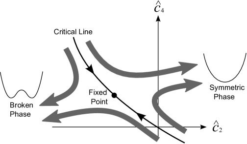
Figure 2: Schematic diagram of the RG flow in the dimensionless parameter space that characterizes the shape of the effective potential. The critical line defines the phase transition, on which the flow runs into the Wilson-Fisher fixed point.

The order of the phase transition and the critical phenomena are characterized by the behavior of the effective action or the flow of the coefficients $c_{i}$ in Eq. (10). Let us consider a coarse-grained action $\Gamma_{k}^{\text{glue}}$ at some momentum scale $k$, which is defined by an effective action with the quantum and thermal fluctuations above $k$ integrated out (see also Sec. 4.2.2 for a theoretical framework). The full effective action is therefore retrieved in the $k\to 0$ limit. Then, naturally, the coefficients are dependent on $k$ as well as $T$, that is, $c_{i}(T;k)$. To take account of the rescaling process in the renormalization group (RG) equation, we make these coefficients dimensionless using $k$ and denote them as $\hat{c}_{i}$.

If the phase transition is of second order, with decreasing $k$, these dimensionless $\hat{c}_{i}$’s flow toward an infrared (IR) fixed point along the critical line (or hypersurface in general), as schematically illustrated in Fig. 2. As $T$ changes, the initial point of the RG flow moves, and when it crosses the critical hypersurface, the destination of the flow drastically changes from the broken phase (with $\hat{c}_{2}\to-\infty$) to the symmetric phase (with $\hat{c}_{2}\to+\infty$). If the initial point sits exactly on the critical hypersurface, the flow heads for the IR (Wilson-Fisher) fixed point that describes the second-order critical point, and the critical phenomena are uniquely determined by the flow pattern near the fixed point. That is, according to the general theory of critical phenomena, the critical behavior associated with the second-order phase transition (approaching $T_{\text{c}}$ from the ordered phase) is characterized by

$$\Phi\propto\langle\ell(\boldsymbol{x})\rangle\propto t^{\beta}\;\;,\quad\chi\propto t^{-\gamma}\;,\quad C\propto t^{-\alpha}\;,\quad\xi\propto t^{-\nu}\;,\quad\langle\ell(0)\ell(\boldsymbol{x})\rangle\propto\frac{1}{|\boldsymbol{x}|^{d-2+\eta}}$$ (11)

as a function of the reduced temperature, $t=|T-T_{\text{c}}|/T_{\text{c}}$. The critical behavior of the order parameter is specified by $\beta$, the susceptibility $\chi$ by $\gamma$, the specific heat $C$ by $\alpha$, and the correlation length $\xi$ by $\nu$. The two-point spatial correlation function $\langle\ell(0)\ell(\boldsymbol{x})\rangle$ has an anomalous dimension $\eta$ at $T=T_{\text{c}}$. These critical exponents are not all independent but they satisfy the scaling relations;

(Rushbrooke scaling) $$\alpha+2\beta+\gamma=2$$  ,

(Fisher scaling)  ,

(Josephson scaling)  .

(12)

It has been established that the properties near the IR fixed point can be classified with the global symmetry of the theory and the spatial dimensions $d$ and this idea of the classification is commonly referred to as the universality. In scalar theories in particular, $d=4$ is known as the critical dimension. The IR fixed point moves to the origin when $d\to 4$, and eventually merges with a ultraviolet (UV) fixed point right at $d=4$. When $d>4$, the fixed point goes across the origin and is hidden in the unstable and unphysical region with $\hat{c}_{4}<0$. Then, the flow goes into the Gaussian fixed point at the origin that describes a free theory, so that the critical exponents take the classical (mean-field) values (see Tab. 1).

According to the universality argument, the deconfinement phase transition in ($d$+1) dimensions can be analyzed by a scalar theory sharing the same global symmetry (i.e. $\mathrm{Z}_{N_{\text{c}}}$ center symmetry) in $d$ dimensions [44, 45]. The critical exponents can be deduced in a simpler theory than the Yang-Mills theory if the phase transition is of second order described by the same IR fixed point (Svetitsky-Yaffe conjecture). The key point is that this argument gives us the critical exponents, but it does not guarantee anything about the order of the phase transition. Table 1 summarizes the Svetitsky-Yaffe prediction for the critical exponents and the results of the numerical tests.

Spatial dimension	Gauge group	Svetitsky-Yaffe conjecture		Numerical test
$d=2$	$\mathrm{U(1)}$ $\mathrm{Z}(N>4)$ $\mathrm{SU}(N>4)$	(KT)   $\eta=1/4$
	$\mathrm{Z(2),\;Z(4)}$ $\mathrm{SU(2)}$	$\beta=0.125$ $\gamma=1.75$ $\alpha=0$	$\nu=1$ $\eta=0.25$	(Universal Second Order) [46]
	$\mathrm{SU(4)}$	(Varying Exponents)		(Second Order) [47]
	$\mathrm{Z(3)}$ $\mathrm{SU(3)}$	$\beta=0.11$ $\gamma=1.44$ $\alpha=0.33$	$\nu=0.83$ $\eta=0.27$	(Universal Second Order) [48]
$d=3$	$\mathrm{U(1)}$ $\mathrm{Z}(N\geq 4)$ $\mathrm{SU}(N\geq 4)$	$\beta=0.35$ $\gamma=1.32$ $\alpha=-0.01$	$\nu=0.67$ $\eta=0.03$	(First Order) [49]
	$\mathrm{Z(2)}$ $\mathrm{SU(2)}$	$\beta=0.33$ $\gamma=1.24$ $\alpha=0.11$	$\nu=0.63$ $\eta=0.03$	(Universal Second Order) [50]
	$\mathrm{Z(3)}$ $\mathrm{SU(3)}$	(First Order)		(First Order) [51]
$d\geq 4$	$\mathrm{U(1)}$ $\mathrm{Z}(N\neq 3)$ $\mathrm{SU}(N\neq 3)$	$\beta=1/2$ $\gamma=1$ $\alpha=0$	$\nu=1/2$ $\eta=0$
	$\mathrm{Z(3)}$ $\mathrm{SU(3)}$	(First Order)

Table 1: Svetitsky-Yaffe conjecture for various gauge theories and the numerical test in the lattice simulation. KT in $d=2$ represents the Kosterlitz-Thouless transition. Table adapted from Ref. [45].

The situation relevant to QCD of our interest is the $\mathrm{SU}(N_{\text{c}})$ case at $d=3$. The universal behavior of the second-order phase transition has been confirmed in the numerical simulation of the $\mathrm{SU(2)}$ Yang-Mills theory. In the $N_{\text{c}}=3$ case, the effective scalar theory does not have a stable IR fixed point, which implies that the phase transition is possibly of first order. Indeed the $\mathrm{SU(3)}$ Yang-Mills theory has turned out to exhibit a first-order phase transition in the numerical simulation. The situation is subtle for $N_{\text{c}}\geq 4$. One may think that the corresponding scalar theory with $\mathrm{Z}(N_{\text{c}})$ symmetry may have a first-order phase transition, but this $\mathrm{Z}(N_{\text{c}})$ symmetry is dynamically enhanced to $\mathrm{U}(1)$ symmetry at the critical point, and then a second-order phase transition is theoretically possible as listed in the Svetitsky-Yaffe conjecture. It has been, however, established that the order of the phase transition is not second but first for the $\mathrm{SU}(6)$ and $\mathrm{SU}(8)$ Yang-Mills theories. Hence, the gauge theories at $N_{\text{c}}\geq 4$ seem not to fall into the Svetitsky-Yaffe universality class. References for the lattice simulations are listed in Tab. 1.

2.2 Flavor symmetry

The quark part in the QCD Lagrangian density (1) has global symmetries in flavor space. Because the gauge part is not sensitive to the flavor structure, we can safely concentrate on the quark part in what follows.

A quark field $\psi$ is decomposed into two chiral sectors,

$$\psi_{\text{L}}\equiv\frac{1-\gamma_{5}}{2}\psi\;,\qquad\psi_{\text{R}}\equiv\frac{1+\gamma_{5}}{2}\psi\;.$$ (13)

The quark Lagrangian density is then expressed in terms of $\psi_{\text{L,R}}$, that reads,

$$\bar{\psi}(i\gamma^{\mu}D_{\mu}-\boldsymbol{m})\psi=\bar{\psi}_{\text{L}}i\gamma^{\mu}D_{\mu}\psi_{\text{L}}+\bar{\psi}_{\text{R}}i\gamma^{\mu}D_{\mu}\psi_{\text{R}}-\bar{\psi}_{\text{L}}\boldsymbol{m}\psi_{\text{R}}-\bar{\psi}_{\text{R}}\boldsymbol{m}\psi_{\text{L}}\;,$$ (14)

where we suppressed the color and the flavor indices to simplify the notation. The covariant derivative is defined as usual as $(D_{\mu})_{ij}=\partial_{\mu}\delta_{ij}-igA_{\mu}^{a}T^{a}_{ij}$ and the mass matrix takes the form of $\boldsymbol{m}=\text{diag}(m_{\text{u}},m_{\text{d}},m_{\text{s}},\dots)$ in flavor space.

Here let us assume the chiral limit in which there are $N_{\text{f}}$ massless flavors ($m_{\text{u}}=m_{\text{d}}=m_{\text{s}}=\dots=0$). In the chiral limit the left- and right-handed sectors are totally disconnected from each other and any mixing between $\psi_{\text{L}}$ and $\psi_{\text{R}}$ is forbidden on the Lagrangian level. Therefore, the Lagrangian density is invariant under two independent chiral rotations by

$$\begin{array}[]{lp{1em}l}\psi_{\text{L}}\;\to\;\psi_{\text{L}}^{\prime}=L\,\psi_{\text{L}}\;,&&\psi_{\text{R}}\;\to\;\psi_{\text{R}}^{\prime}=R\,\psi_{\text{R}}\;,\\ L=\exp\bigl{(}i\theta_{\text{L}}^{a}t^{a}\bigr{)}\>\in\;\mathrm{U}(N_{\text{f}})_{\text{L}}\;,&&R=\exp\bigl{(}i\theta_{\text{R}}^{a}t^{a}\bigr{)}\>\in\;\mathrm{U}(N_{\text{f}})_{\text{R}}\;,\end{array}$$ (15)

where $t^{a}$’s denote the $\mathrm{su}(N_{\text{f}})$ algebras and the flavor index runs over $a=1,\cdots,N_{\text{f}}^{2}-1$. This means that the QCD Lagrangian density has the following symmetry,

$$\mathrm{U}(N_{\text{f}})_{\text{L}}\times\mathrm{U}(N_{\text{f}})_{\text{R}}\;\;\simeq\;\;\mathrm{SU}(N_{\text{f}})_{\text{L}}\times\mathrm{SU}(N_{\text{f}})_{\text{R}}\times\mathrm{U}(1)_{\text{V}}\times\mathrm{U}(1)_{\text{A}}\;,$$ (16)

apart from the discrete symmetry. (The center elements of $\mathrm{SU}(N_{\text{f}})$ also belong to $\mathrm{U}(1)$, and so $\mathrm{Z}(N_{\text{f}})$ is redundant in the right-hand side above; see Ref. [18].)

Realization of the global symmetry always leads to the existence of the conserved Nöther current. Under the infinitesimal (coordinate dependent) transformations $\psi_{\text{L}}^{\prime}\simeq(1+i\delta\theta_{\text{L}}^{a}(x)t^{a})\psi_{\text{L}}$ and $\psi_{\text{R}}^{\prime}\simeq(1+i\delta\theta_{\text{R}}^{a}(x)t^{a})\psi_{\text{R}}$, the change in the Lagrangian density should be at most the surface term, $\delta\mathcal{L}=\theta_{\text{L}}^{a}(x)\partial_{\mu}j_{\text{L}}^{\mu\,a}(x)+\theta_{\text{R}}^{a}(x)\partial_{\mu}j_{\text{R}}^{\mu\,a}(x)$, where

$$j_{\text{L}}^{\mu\,a}=\bar{\psi}_{\text{L}}\gamma^{\mu}t^{a}\psi_{\text{L}}\;,\qquad j_{\text{R}}^{\mu\,a}=\bar{\psi}_{\text{R}}\gamma^{\mu}t^{a}\psi_{\text{R}}\;.$$ (17)

Then we can make appropriate combinations corresponding to the vector and the axial-vector transformations, i.e.

$$Q_{\text{V}}^{a}=Q_{\text{R}}^{a}+Q_{\text{L}}^{a}\;,\qquad Q_{\text{A}}^{a}=Q_{\text{R}}^{a}-Q_{\text{L}}^{a}\;,$$ (18)

where we defined $Q_{\text{L,R}}^{a}=\int d^{3}x\,\psi_{\text{L,R}}^{\dagger}t^{a}\psi_{\text{L,R}}$.

2.2.1 Chiral symmetry

Among the global symmetry (16) the first part of $\mathrm{SU}(N_{\text{f}})_{\text{L}}\times\mathrm{SU}(N_{\text{f}})_{\text{R}}$ is called chiral symmetry specifically. We postpone the discussions on the remaining part of $\mathrm{U}(1)_{\text{L}}\times\mathrm{U}(1)_{\text{R}}$. Here we give a concise primer of spontaneous chiral symmetry breaking and associated low-energy theorems.

So far, we have seen what symmetries the QCD Lagrangian density possesses. However, the chiral invariance is not manifest in the low-lying hadron spectra where any degenerate patterns between parity partners are absent. The resolution is that chiral symmetry is dynamically broken due to the strong interaction. The generator of the axial transformation, $Q_{\text{A}}^{a}$, does not annihilate the ground state then. In a precise expression, some operator $\mathcal{O}(x)$ exists so that

$$\langle\Omega|\bigl{[}iQ_{\text{A}}^{a},\mathcal{O}(x)\bigr{]}|\Omega\rangle\neq 0\;,$$ (19)

where $|\Omega\rangle$ is the physical state. The symmetry generated by $Q_{\text{A}}^{a}$ is spontaneously broken in this state $|\Omega\rangle$ if Eq. (19) holds, and the above non-zero expectation value is nothing but the order parameter. The simplest choice would be $\mathcal{O}=\bar{\psi}t^{a}\psi$, leading to the chiral condensate as an order parameter;

$$\langle\bar{\psi}\psi\rangle=\langle\bar{\psi}_{\text{L}}\psi_{\text{R}}+\bar{\psi}_{\text{R}}\psi_{\text{L}}\rangle\neq 0\;.$$ (20)

Since $\bar{\psi}\psi$ is unchanged under $\mathrm{SU}(N_{\text{f}})_{\text{V}}$ transformation generated by $Q_{\text{V}}^{a}$, the physical state is invariant and $Q_{\text{V}}^{a}|\Omega\rangle=0$, which obeys the Vafa-Witten theorem [52]. In summary, chiral symmetry is spontaneously broken by $\langle\bar{\psi}\psi\rangle\neq 0$ as

$$\mathrm{SU}(N_{\text{f}})_{\text{L}}\times\mathrm{SU}(N_{\text{f}})_{\text{R}}\;\;\to\;\;\mathrm{SU}(N_{\text{f}})_{\text{V}}\;.$$ (21)

The physical manifestation of such spontaneous symmetry breaking is the presence of massless scalar particles, namely, the Nambu-Goldstone (NG) bosons. In QCD the pions are identified as the approximate NG bosons. We note that the original theory contains only fermions with spin $1/2$ and gauge bosons with spin $1$ and, therefore, the NG bosons must be composite states generated through non-perturbative dynamics. The number of NG bosons is specified by the dimension of the $G/H$ manifold, where $G=\mathrm{SU}(N_{\text{f}})_{\text{L}}\times\mathrm{SU}(N_{\text{f}})_{\text{R}}$ is the original chiral symmetry whereas $H=\mathrm{SU}(N_{\text{f}})_{\text{V}}$ the unbroken vectorial symmetry; there appear as many NG bosons as $\text{dim}(G/H)=N_{\text{f}}^{2}-1$.

The axial current, $J_{\text{A}}^{\mu\,a}$, has a direct coupling to the NG boson $\pi^{b}$, the strength of which can be parametrized by the decay constant $f_{\pi}$ as

$$\langle\Omega|J_{\text{A}}^{\mu\,a}(0)|\pi^{b}(q)\rangle=if_{\pi}q^{\mu}\,\delta^{ab}\;.$$ (22)

In the experimental point of view $f_{\pi}$ is a useful measure, and the empirical value is $f_{\pi}=(92.4\pm 0.2)\;\text{MeV}$. In a medium $f_{\pi}$ serves as an order parameter for (partial) chiral symmetry restoration. The divergence of the axial current is non-vanishing due to an explicit symmetry breaking by the presence of $m_{\text{q}}$, i.e.

$$\partial_{\mu}J_{\text{A}}^{\mu\,a}=f_{\pi}m_{\pi}^{2}\pi^{a}\;,$$ (23)

which is known as the partially conserved axial-vector current (PCAC). If the explicit breaking is turned off, the pion is precisely massless as dictated by the NG theorem and thus the axial current is conserved. Utilizing the PCAC and the soft pion theorems, one can derive low-energy theorems. The most well-known is the Gell-Mann–Oakes–Renner (GOR) relation,

$$f_{\pi}^{2}m_{\pi}^{2}=-m_{\text{q}}\langle\bar{\psi}\psi\rangle\;,$$ (24)

and another important low-energy theorem is the Goldberger–Treiman relation, $f_{\pi}\,g_{\pi NN}=m_{N}\,g_{A}$, where $g_{\pi NN}$ is the pion-nucleon coupling, $m_{N}$ is the nucleon mass, and $g_{A}$ is the nucleon axial charge.

2.2.2 $\mathrm{U(1)_{A}}$ symmetry and the quantum anomaly

The QCD Lagrangian density (1) has not only chiral symmetry $\mathrm{SU}(N_{\text{f}})_{\text{L}}\times\mathrm{SU}(N_{\text{f}})_{\text{R}}$ but also $\mathrm{U}(1)_{\text{V}}\times\mathrm{U}(1)_{\text{A}}$. The $\mathrm{U}(1)_{\text{V}}$ symmetry corresponds to the baryon number conservation and should not be broken except in color-superconductivity at asymptotically high density. Then, according to the NG theorem, there should be one more massless boson associated with the $\mathrm{U(1)_{A}}$ symmetry breaking. There is, however, no such light particle in the iso-singlet pseudo-scalar channel. Instead of the NG boson, the lightest meson in this channel is $\eta^{\prime}$ whose mass is $m_{\eta^{\prime}}=958\;\text{MeV}$, that is too heavy to be the NG boson. The problem of missing $\mathrm{U(1)_{A}}$ NG boson is called the $\mathrm{U(1)_{A}}$ problem.

Now it is a textbook knowledge that the $\mathrm{U(1)_{A}}$ symmetry in the classical Lagrangian is explicitly broken via quantum effects. Such quantum anomaly appears ubiquitously in the gauge field theory. If we choose to adhere the vector gauge symmetry, the quantum anomaly arises in the axial current generally as

$$\partial_{\mu}j_{\text{A}}^{\mu\,a}=-\frac{g^{2}}{16\pi^{2}}\epsilon^{\mu\nu\rho\sigma}\text{tr}\bigl{[}t^{a}\,F_{\mu\nu}F_{\rho\sigma}\bigr{]}\;,$$ (25)

which is non-vanishing only for $a=0$ (iso-singlet) because $t^{a}$’s are traceless for $a=1,\dots,N_{\text{f}}^{2}-1$. Therefore the chiral symmetry breaking pattern is truly the one given by Eq. (21) and $\eta^{\prime}$ cannot be the NG boson. We make a remark here that it is not such easy to disprove the existence of the massless pole because $J_{\text{A}}^{\mu\,0}$ can be modified into a conserved but gauge-variant form. Interested readers can consult Ref. [53].

From the microscopic point of view $\mathrm{U(1)_{A}}$ symmetry is broken through the instanton-induced interactions. Let us take a look at the derivation with an assumption that an instanton with the size $\rho$ is placed at $z$ [54]. Then, the partition function can be expressed in a form of the functional integration over the collective coordinates as

$$Z=\int d^{4}z\,d\rho\,\rho^{-1}(\det D[\mathcal{A}])^{-1/2}(\det G[\mathcal{A}])\,e^{-8\pi^{2}/g^{2}}\;,$$ (26)

after the one-loop integration around the instanton background $\mathcal{A}(x)$. Here $D[\mathcal{A}]$ and $G[\mathcal{A}]$ are the gluon and the (massless) quark propagator inverse, respectively, in the presence of the background $\mathcal{A}(x)$.

It is important to note that a fermionic zero-mode is accompanied by the instanton gauge configuration, which has definite chirality in accord with the sign of the winding number $Q_{\text{W}}$; for $\mathcal{A}(x)$ with $Q_{\text{W}}=1$ for instance, there exists a wave-function that satisfies $G[\mathcal{A}]\psi_{\text{R}0}=0$ (apart from the mass term). Therefore, the partition function $Z$ should be zero in this case. Now we deform the theory slightly so that $Z$ stays finite, that is, we insert a source term, $\bar{\psi}_{\text{L}}J(x)\psi_{\text{R}}$, in the fermionic part $G$. Then, at low energies, we can approximate the Dirac determinant as

$$\det[G+J]\;\simeq\;\det\int d^{4}x\,\bar{\psi}_{\text{L}0}J(x)\psi_{\text{R}0}\;.$$ (27)

Here det in the right-hand side is taken in flavor space. Now we shall consider an effective theory of QCD with all gluonic fields integrated out. Then this effective theory should be written in terms of quark fields $\bar{\psi}(x)$ and $\psi(x)$. The question is how to incorporate the instanton effect with the quark degrees of freedom only, or how to find an effective interaction vertex induced by instanton. We can find such an instanton-induced interaction to reproduce Eqs. (26) and (27); the following vertex can mimic Eq. (27) and thus embody the instanton effect;

$$\mathcal{L}_{\mathrm{U(1)_{A}}}\sim n(\rho,T=0)\,\bigl{[}\det\bar{\psi}(1-\gamma^{5})\psi+\det\bar{\psi}(1+\gamma^{5})\psi\bigr{]}\;,$$ (28)

including the latter term coming from an anti-instanton. As expected, the interaction (28) breaks the $\mathrm{U(1)_{A}}$ symmetry explicitly, while chiral $\mathrm{SU}(N_{\text{f}})_{\text{L}}\times\mathrm{SU}(N_{\text{f}})_{\text{R}}$ symmetry is kept unbroken. This determinant form had been postulated earlier from the symmetry consideration [55] and the above interaction (28) is now called the Kobayashi-Maskawa-’t Hooft (KMT) interaction.

In the above derivation it is clear that the interaction strength is proportional to the instanton density that is given in the one-loop perturbation theory by

$$n(\rho,T=0)=\frac{8\pi^{2}}{g^{2}}\,\rho^{-5}e^{-8\pi^{2}/g^{2}}\;,$$ (29)

originating from $\det D[\mathcal{A}]$. Thus, the strength of the $\mathrm{U(1)_{A}}$ breaking interaction depends on how many instantons the system would accommodate, though the anomaly itself is never diminished and Eq. (25) is not altered by the finite-$T$ effect. This fact opens an interesting possibility. That is, at finite $T$, the one-loop instanton density is modified as [56],

$$n(\rho,T)=\biggl{(}\frac{8\pi^{2}}{g^{2}}\,\rho^{-5}e^{-8\pi^{2}/g(\rho)^{2}}\biggr{)}\,\exp\biggl{[}-\pi^{2}\rho^{2}T^{2}\biggl{(}\frac{2N_{\text{c}}}{3}+\frac{N_{\text{f}}}{3}\biggr{)}\biggr{]}\;.$$ (30)

The latter exponential factor suppresses the instanton excitation significantly. Similarly, at finite density, the exponential suppression factor has been found [57], and after integrating over the instanton size, the suppression factor should be $T^{-14}$ or $\mu^{-14}$. In any case these expressions are perturbative ones, and any quantitative estimate is not really trustworthy near $T_{\text{c}}$. Nevertheless, it is quite suggestive that $n(T\sim T_{\text{c}})$ in the above expression is already a half of $n(T=0)$. Then, one may well speculate that the $\mathrm{U(1)_{A}}$ symmetry is effectively restored before the critical temperature/density is reached [58], and if so, as we will see in the next subsection, the universality class and the critical properties would be significantly affected.

2.2.3 Chiral phase transition and critical phenomena

The order of the chiral phase transition was systematically investigated first by the RG analysis [59]. As we explained, if the phase transition is of second order, the fixed-point structure yields the critical exponents not relying on the microscopic dynamics. One can also say that, reversely, the absence of the stable fixed point suggests that the theory should exhibit a first-order phase transition.

To clarify the nature of the phase transition we need not to solve QCD at finite temperature but we can make use of an effective description with chiral symmetry. The simplest model is the linear sigma model composed from the meson field matrices, $M_{ij}\sim\bar{\psi}_{\text{R}j}\psi_{\text{L}i}$ and its conjugate $M^{\dagger}$ that transform as

$$M\;\to\;L^{\dagger}MR\;,\qquad M^{\dagger}\;\to\;R^{\dagger}M^{\dagger}L\;.$$ (31)

The general Lagrangian density consistent with chiral symmetry is decomposed into $\mathcal{L}=\mathcal{L}_{\sigma}+\mathcal{L}_{\mathrm{U(1)_{A}}}+\mathcal{L}^{\prime}$, where

$$\mathcal{L}_{\sigma}=\frac{1}{2}\text{tr}\bigl{(}\partial_{\mu}M\partial^{\mu}M^{\dagger}\bigr{)}+\frac{1}{2}\mu^{2}\text{tr}\bigl{(}MM^{\dagger}\bigr{)}-\frac{\pi^{2}g_{1}}{3}\bigl{[}\text{tr}\bigl{(}MM^{\dagger}\bigr{)}\bigr{]}^{2}-\frac{\pi^{2}g_{2}}{3}\text{tr}\bigl{(}MM^{\dagger}MM^{\dagger}\bigr{)}\;,$$ (32)

and the instanton-induced KMT interaction $\mathcal{L}_{\mathrm{U(1)_{A}}}=c\bigl{(}\det M+\det M^{\dagger}\bigr{)}$ which is reminiscent of Eq. (28), and the explicit breaking part $\mathcal{L}^{\prime}=f_{0}\,\text{tr}(t^{0}M)+f_{3}\,\text{tr}(t^{3}M)+f_{8}\,\text{tr}(t^{8}M)+\cdots$ ranging over all the Cartan subalgebras. Here, in $\mathcal{L}_{\sigma}$, the first is the kinetic term, the second is the mass term, and the third and the fourth are potential terms that results in the spontaneous symmetry breaking, respectively. From the symmetry property $M$ can be decomposed as

$$M=\Sigma+i\Pi=\sum_{a=0}^{N_{\text{f}}^{2}-1}t^{a}(\sigma_{a}+i\pi_{a})$$ (33)

with the scalar fields, $\Sigma=t^{a}\sigma_{a}=\tfrac{1}{2}(M+M^{\dagger})$, and the pseudo-scalar fields, $\Pi=t^{a}\pi_{a}=\tfrac{1}{2i}(M-M^{\dagger})$. (Note that $M$ changes to $M^{\dagger}$ under the parity transformation.) Because $M$ transforms as $V^{\dagger}MV$ under a vectorial rotation ($V=L=R$), one can classify the matrix components in terms of the hadron language. In the $N_{\text{c}}=3$ case, for example,

$$\begin{split}&\Sigma=\begin{pmatrix}\frac{1}{\sqrt{2}}(\sigma+a_{0}^{0})&a_{0}^{+}&K^{\ast+}\\ a_{0}^{-}&\frac{1}{\sqrt{2}}(\sigma-a_{0}^{0})&K^{\ast 0}\\ K^{\ast-}&\bar{K}^{\ast 0}&\zeta\end{pmatrix}\;,\\ &\Pi=\begin{pmatrix}\frac{1}{\sqrt{2}}\pi^{0}+\frac{1}{\sqrt{6}}\eta_{8}+\frac{1}{\sqrt{3}}\eta_{0}&\pi^{+}&K^{+}\\ \pi^{-}&-\frac{1}{\sqrt{2}}\pi^{0}+\frac{1}{\sqrt{6}}\eta_{8}+\frac{1}{\sqrt{3}}\eta_{0}&K^{0}\\ K^{-}&\bar{K}^{0}&-\frac{2}{\sqrt{6}}\eta_{8}+\frac{1}{\sqrt{3}}\eta_{0}\end{pmatrix}\end{split}$$ (34)

with two independent condensates $\sigma$ and $\zeta$ (isospin symmetry is assumed) corresponding to two chiral condensates, $\langle\bar{u}u\rangle=\langle\bar{d}d\rangle$ and $\langle\bar{s}s\rangle$. In this case $\eta_{0}$ is anomalous, while there are eight NG bosons, $\pi^{0}$, $\pi^{\pm}$, $K^{0}$, $\bar{K}^{0}$, $K^{\pm}$, and $\eta_{8}$, in the chiral limit. In reality $\mathrm{SU}(3)_{\text{V}}$ symmetry is substantially broken by the strange quark mass $m_{\text{s}}$, so that the masses in the strange sector, $K^{0}$, $\bar{K}^{0}$, $K^{\pm}$, $\eta_{8}$, are lifted up by $m_{\text{s}}$. Besides, $\eta_{8}$ and $\eta_{0}$ can mix together by $m_{\text{s}}$, which amounts to physical states of $\eta$ and $\eta^{\prime}$.

One could put this linear sigma model directly in a finite-$T$ environment and investigate the phase transition of chiral restoration. For the present purpose to study the order of the phase transition and the critical properties, however, the universality argument is extremely useful. It is sufficient to begin with a dimensionally reduced description after the integration over temperature fluctuations, as already discussed in Sec. 2.1.2, and then we can simply focus on the 3-dimensional linear sigma model with $T$-dependent couplings $g_{1}(T;k)$, $g_{2}(T;k)$, $c(T;k)$, etc, at the RG scale $k$. Since we are interested in the critical phenomena only, we shall work in the chiral limit, $f_{0}=f_{3}=f_{8}=\cdots=0$.

Symmetry breaking pattern		Flavors		Pisarski-Wilczek conjecture
$\mathrm{SU}(N_{\text{f}})_{\text{L}}\times\mathrm{SU}(N_{\text{f}})_{\text{R}}\to\mathrm{SU}(N_{\text{f}})_{\text{V}}$		$N_{\text{f}}=2$		$\beta=0.38$ $\gamma=1.44$ $\alpha=-0.19$	$\nu=0.73$ $\eta=0.03$
		$N_{\text{f}}\geq 3$		(First Order)
$\mathrm{SU}(N_{\text{f}})_{\text{L}}\times\mathrm{SU}(N_{\text{f}})_{\text{R}}\times\mathrm{U}(1)_{\text{A}}\to\mathrm{SU}(N_{\text{f}})_{\text{V}}$		$N_{\text{f}}=1$		$\beta=0.35$ $\gamma=1.32$ $\alpha=-0.015$	$\nu=0.67$ $\eta=0.038$
		$N_{\text{f}}\geq 2$		(First Order)

Table 2: Pisarski-Wilczek conjecture for the chiral phase transition in $d=3$ space.

Without the axial anomaly

Let us first consider the case without the $\mathrm{U(1)_{A}}$-breaking term (i.e. $c=0$). This is possible if the effective restoration of $\mathrm{U(1)_{A}}$ symmetry occurs slightly below $T_{\text{c}}$ due to instanton suppression as argued in Sec. 2.2.2. In this case the symmetry breaking pattern is

$$\mathrm{U}(N_{\text{f}})_{\text{L}}\times\mathrm{U}(N_{\text{f}})_{\text{R}}\;\;\to\;\;\mathrm{U}(N_{\text{f}})_{\text{V}}\;,$$ (35)

and there are $N_{\text{f}}^{2}$ massless NG bosons. The critical phenomena can be analyzed by the $\epsilon$ expansion, in which the spatial dimension is taken as $d=4-\epsilon$ and $\epsilon$ is assumed to be a small number. Because $d=4$ is the critical dimension, the coupling constant around the fixed point is $\sim\mathcal{O}(\epsilon)$, which justifies the perturbation theory.

One can then carry out the one-loop calculation using the Lagrangian (32) to find the following $\beta$ functions;

$$\begin{split}&\beta_{1}\equiv k\frac{d\hat{g}_{1}}{dk}=-\epsilon\hat{g}_{1}+\frac{N_{\text{f}}^{2}+4}{3}\hat{g}_{1}^{2}+\frac{4N_{\text{f}}}{3}\hat{g}_{1}\hat{g}_{2}+\hat{g}_{2}^{2}\;,\\ &\beta_{2}\equiv k\frac{d\hat{g}_{2}}{dk}=-\epsilon\hat{g}_{2}+2\hat{g}_{1}\hat{g}_{2}+\frac{2N_{\text{f}}}{3}\hat{g}_{2}^{2}\end{split}$$ (36)

for general $N_{\text{f}}$. We introduced a notation for the dimensionless couplings, $\hat{g}_{1}=g_{1}k^{-\epsilon}$ and $\hat{g}_{2}=g_{2}k^{-\epsilon}$. The first term in the right-hand side of Eq. (36) involving $\epsilon$ appears trivially from $k^{-\epsilon}$ in $\hat{g}_{1}$ and $\hat{g}_{2}$. One can solve this set of differential equations to draw the RG flow pattern. The fixed points can be found readily from the conditions, $\beta_{1}=\beta_{2}=0$. Two solutions always exist, one at $(\hat{g}_{1}^{\ast},\hat{g}_{2}^{\ast})=(0,0)$, and the other at

$$(\hat{g}_{1}^{\ast},\hat{g}_{2}^{\ast})=\Bigl{(}\frac{3\epsilon}{N_{\text{f}}^{2}+4},0\Bigr{)}\;,$$ (37)

and two more fixed-points can appear for $N_{\text{f}}\leq\sqrt{3}$ at

$$(\hat{g}_{1}^{\ast},\hat{g}_{2}^{\ast})=\frac{3\epsilon}{2(27-8N_{\text{f}}^{2}+N_{\text{f}}^{4})}\biggl{(}9-N_{\text{f}}^{2}\mp N_{\text{f}}\sqrt{2(3-N_{\text{f}}^{2})}\;,\;-5N_{\text{f}}+N_{\text{f}}^{3}\pm 3\sqrt{2(3-N_{\text{f}}^{2})}\biggr{)}\;.$$ (38)

From explicit analysis it turns out that Eq. (37) is an IR-stable fixed point for $0\leq N_{\text{f}}\leq\sqrt{2}$, and then this fixed point would represent the critical phenomena of the $\mathrm{O}(2N_{\text{f}})$ universality class (which is rather close to the situation with the axial anomaly). Therefore, when $N_{\text{f}}=1$, the phase transition can be of second order, and if so, it is characterized by the $\mathrm{O}(2)$ critical exponents. For $N_{\text{f}}>\sqrt{3}$ this fixed-point becomes unstable in the $\hat{g}_{2}$ direction and there is no IR-stable fixed-point at all. Thus, when $N_{\text{f}}\geq 2$, it is impossible to have a second-order phase transition and it should be of fluctuation-induced first order.

One might have had an impression that the leading-order $\epsilon$ expansion is insufficient to conclude whether the phase transition is of first order. It should be mentioned that this conclusion of the fluctuation-induced first-order transition has been confirmed non-perturbatively in a more sophisticated framework of the functional RG method [60, 61].

With the axial anomaly

If the instanton-induced $\mathrm{U(1)_{A}}$-breaking interaction remains non-vanishing, as is a more conventional scenario, the critical properties are drastically changed especially in the case with $N_{\text{f}}=2$. Because, in the $N_{\text{f}}=2$ case, the original group is $\mathrm{SU}(2)_{\text{L}}\times\mathrm{SU}(2)_{\text{R}}\simeq\mathrm{O}(4)$, the critical phenomena should belong to the $\mathrm{O}(4)$ universality class. This can be analyzed in the $\epsilon$ expansion in the same way as previously. The instanton term $\det M+\det M^{\dagger}$ yields substantial mass terms for the scalar particles only, and $\Sigma$ decouples from the low-lying dynamics. Then, with only $\Pi$, two terms involving $g_{1}$ and $g_{2}$ in Eq. (32) are no longer independent, and the $\beta$ function is reduced to $\beta_{1}$ in Eq. (36) with $\hat{g}_{2}=0$, which has a stable fixed-point unlike the previous case without the anomaly.

For $N_{\text{f}}\geq 3$ no IR-stable fixed point is found, and it is likely that the phase transition is of first order. In fact, even at the tree level, the KMT interaction at $N_{\text{f}}=3$ involves terms like $\sigma^{3}$ in the chiral limit where $\zeta=\sigma$. The presence of such cubic term strongly implies that the phase transition should be of first order.

To summarize the expected critical properties of the chiral phase transition in $d=3$ space, we shall make a table based on this Pisarski-Wilczek conjecture [59] as in Tab. 2.

2.3 Highlights of the lattice-QCD results

In this subsection let us look over the numerical results from the Monte-Carlo simulation of QCD on the lattice. Although there are some data available for spatially 2-dimensional case, we will limit our discussions here to the realistic situation with $d=3$ in space. For details on the lattice-QCD simulation, readers may consult Refs. [62, 63].

Pure Yang-Mills theories

The left panel of Fig. 3 shows a figure adapted from Ref. [64] for the renormalized Polyakov loop in various representations in color space. It is the renormalization effect that renders $\Phi$ exceed the unity. We see that the order parameter clearly shows a discontinuous jump at $T=T_{\text{c}}$. (We should note that $\Phi=0$ below $T_{\text{c}}$ where center symmetry is unbroken which is omitted in Fig. 3.) In the pure Yang-Mills theory the physical scale is set with the string tension $\sigma$, and the critical temperature is found as $T_{\text{c}}=(0.630\pm 0.005)\sqrt{\sigma}\simeq 280\;\text{MeV}$ [65]. In the right panel of Fig. 3 a figure adapted from Ref. [66] presents thermodynamic quantities such as the internal energy density $\varepsilon$ and the pressure $p$ for the pure Yang-Mills theories with various gauge groups. From this figure we can understand that the thermodynamics has only weak dependence on the number of colors once properly normalized by the Stefan-Boltzmann value (for more general large-$N_{\text{c}}$ studies, see Refs. [67, 68]). It is also evident in the behavior of $\varepsilon(T)$ that the physical degrees of freedom rapidly change at $T=T_{\text{c}}$ corresponding to the liberation of colored excitations. On the other hand, the pressure $p$ is always continuous regardless of the order of the phase transition. The state-of-the-art lattice data at high precision is available in Ref. [69]. The blue curves in Fig. 3 represent the potential fit results for later convenience, which we will discuss in Sec. 4.2.1.

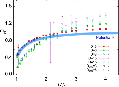
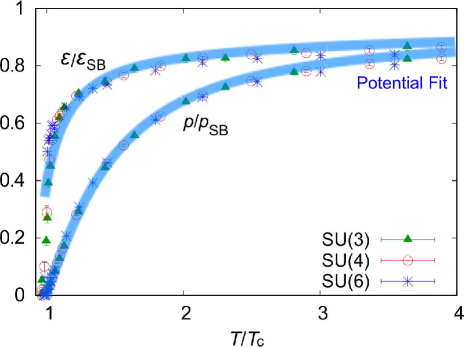
Figure 3: (Left) Renormalized Polyakov loop in various representations (with the dimension $D$) in the SU(3) Yang-Mills theory. The blue curve represents the potential fit from $\Omega_{\text{glue}}[\Phi]$ discussed in Sec. 4.2.1. Figure adapted from Ref. [64]. (Right) Energy density and pressure in the $\mathrm{SU}(N_{\text{c}})$ Yang-Mills theories normalized by the Stefan-Boltzmann value. The blue curves represent the potential fit from $\Omega_{\text{glue}}[\Phi]$ again. Figure adapted from Ref. [66].

Full QCD

Figure 4 is the counterpart of Fig. 3 for the full QCD simulation with dynamical quarks. In this case not only the Polyakov loop $\Phi$ but also the chiral condensate $\langle\bar{\psi}\psi\rangle$ is an interesting quantity and they both show smooth crossover as seen in the left panel of Fig. 4. To conclude that they are crossover in a rigorous way, the finite-volume scaling is necessary [70]. For the practical purpose, it is more appropriate to use a subtracted order parameter at $T$ defined by [71],

$$\Delta_{\text{l},\text{s}}\equiv\frac{M(T)}{M(0)}\;,\qquad M(T)\equiv\hat{m}_{\text{s}}\Bigl{(}\langle\bar{\psi}\psi\rangle_{\text{l}}-\frac{m_{\text{l}}}{m_{\text{s}}}\langle\bar{\psi}\psi\rangle_{\text{s}}\Bigr{)}N_{\tau}^{4}\;,$$ (39)

rather than the naïve chiral condensate, where $\hat{m}_{\text{s}}$ is the strange quark mass in the lattice unit and $N_{\tau}$ is the site number along the temporal direction. This combination is chosen to be free from an additive divergence $\sim m_{\text{q}}\Lambda^{2}$ inherent in the chiral condensate. This subtracted order parameter, $\Delta_{\text{l},\text{s}}$, is plotted in the left panel of Fig. 4.

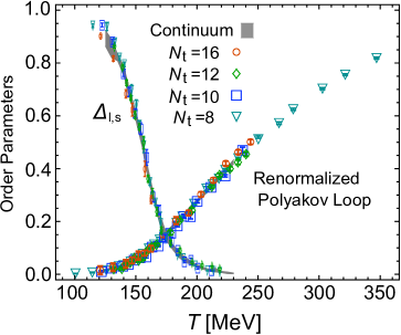
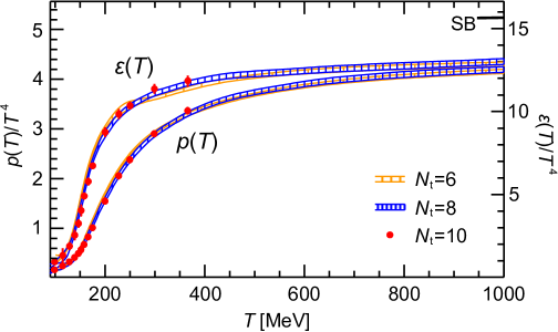
Figure 4: (Left) Renormalized Polyakov loop and the subtracted and normalized chiral condensate in the (2+1)-flavor QCD simulation. The definition of $\Delta_{\text{l},\text{s}}$ is explained in Eq. (39). Figure adapted from Ref. [72] and originally two separate plots are superimposed with the horizontal axis properly adjusted. (Right) Energy density and pressure in the (2+1)-flavor QCD simulation. Figure adapted from Ref. [73] and originally two separate plots are superimposed with the vertical axis adjusted by the Stefan-Boltzmann limit.

Interestingly, as seen from the left panel of Fig. 4, two crossovers of deconfinement and chiral restoration happen almost simultaneously; the renormalized Polyakov loop and $\Delta_{\text{l},\text{s}}$ start increasing and decreasing, respectively, in the same temperature range. One may define the pseudo-critical temperature (see Eq. (40)) but it is not meaningful to ask whether two pseudo-critical temperatures coincide or not quantitatively. As we will discuss later, the chiral crossover is pretty close to the second-order phase transition and critical scaling properties are expected, while the deconfinement crossover spreads over a wide temperature range. In this sense, it is often emphasized that only the chiral restoration is critical and there is no phase transition associated with deconfinement. This statement is indeed true, but we would insist that it is still a highly non-trivial problem how these two crossovers can be such correlated (see Ref. [74] for a possible scenario). In view of the internal energy density, $\varepsilon(T)$, in the right panel of Fig. 4, deconfinement crossover occurs in a narrower window of the temperature than suggested from $\Phi$ in the left panel. We see that the physical degrees of freedom rapidly increase within the temperature range $\lesssim 100\;\text{MeV}$ and the phenomenon of color deconfinement makes reasonable sense though it does not come along with critical scaling. In the same way as the pure gluonic case, the pressure $p(T)$ is a continuous function in the whole $T$ range.

Sometimes, to quantify the crossover location, the pseudo-critical temperature is defined. The pseudo-critical temperature should coincide with the critical temperature when crossover turns to a second-order phase transition in the chiral limit. One should keep in mind that the pseudo-critical temperature is a quantity only for convenience and it does not add any physical insight. There are several different prescriptions which lead to different pseudo-critical temperatures.

A frequently used prescription for the pseudo-critical temperature is to see the peak position of the chiral susceptibility,

$$\chi_{\bar{\psi}\psi}=\frac{T}{V}\frac{\partial^{2}\ln Z}{\partial m_{\text{q}}^{2}}\;,$$ (40)

which gives $T_{\text{c}}=151(3)(3)\;\text{MeV}$ for chiral restoration, where the first error comes from the $T\neq 0$ and the second from $T=0$ analyses [75]. We note that this estimate gives the systematic error but does not have uncertainty from the choice of the prescription. In view of the order parameter behavior in Fig. 4, we should consider that the pseudo-critical temperatures from various definitions could not avoid substantial uncertainty more than $\Delta T_{\text{c}}\sim\pm 20\;\text{MeV}$.

It is obvious at first glance from Fig. 4 that there is no prominent phase transition at all associate with deconfinement in full QCD data, while $\Phi$ serves as a good order parameter in the pure Yang-Mills theories. Thus, the pseudo-critical temperature for deconfinement is less meaningful than that for the chiral phase transition. One way to locate the deconfinement pseudo-critical temperature is to look for the inflexion point of $\Phi(T)$ or the peak position of the temperature derivative of the Polyakov loop, $d\Phi(T)/dT$. This prescription gives an estimate $T_{\text{c}}=176(3)(4)\;\text{MeV}$ [75]. Needless to say, the real uncertainty width should be much larger than the errors, that is, $\Delta T_{\text{c}}\sim\pm 50\;\text{MeV}$ at least from the curve in the left panel of Fig. 4. Another possible way to define the pseudo-critical point is to use the peak position of the Polyakov loop susceptibility in the same manner as for chiral restoration. The left panel of Fig. 5 shows an example at various light quark masses. We can notice a general trend that two pseudo-critical temperatures stick to each other, which is clearer for larger quark mass ($m_{\text{l}}=0.4m_{\text{s}}$) and becomes vague for small (physical) quark mass ($m_{\text{l}}=0.1m_{\text{s}}$). The latest lattice data can be found in Ref. [76].

Instead of the Polyakov loop, it is also possible to utilize the strange quark number susceptibility to define the pseudo-critical temperature;

$$\chi_{\text{s}}=\frac{T}{V}\frac{\partial^{2}\ln Z}{\partial\mu_{\text{s}}^{2}}\;,$$ (41)

where $\mu_{\text{s}}$ is the chemical potential for strange quarks. This quantity, $\chi_{\text{s}}$, behaves in a similar way to the Polyakov loop (see the right panel of Fig. 5), which can be easily understood in a model as commented below Eq. (137). The inflexion point of $\chi_{\text{s}}$ gives the pseudo-critical point consistent with the definition by means of the Polyakov loop, i.e. $T_{\text{c}}=175(2)(4)\;\text{MeV}$ [75].

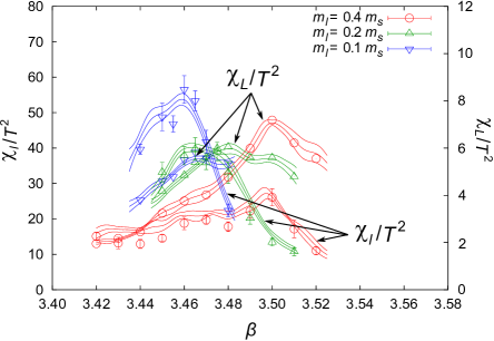
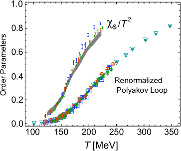
Figure 5: (Left) Peaks in the Polyakov loop susceptibility $\chi_{L}$ and the chiral susceptibility $\chi_{l}$, from which the pseudo-critical temperatures are defined for various quark masses. Figure adapted from Ref. [77] and originally three separate plots are superimposed. (Right) Strange quark number susceptibility in the (2+1)-flavor lattice simulation together with the renormalized Polyakov loop. The pseudo-critical temperature for deconfinement is defined from the inflexion point of the susceptibility with respect to the temperature. Figure adapted from Ref. [75] and originally two separate plots are superimposed.

In the application of the lattice-QCD data to the heavy-ion collision experiment it is crucially important to check how close to criticality the QCD phase transition is. If $u$- and $d$-quarks are massless, the chiral phase transition should be of second order that belongs to the O(4) universality class as argued in Sec. 2.2.3. If the physical quark mass is situated in the critical region, the subtracted order parameter $M$ in Eq. (39) should obey the critical scaling, which can be parametrized in terms of the universality scaling function and scaling variables. The lattice data as reported in Ref. [78, 79] is consistent with the O(4) or O(2) universality class. (The O(2) universality class is also expected for the coarse staggered fermion.) Therefore, the pseudo-critical temperature for chiral restoration conveys a definite meaning if it is fixed such that the magnetic equation of state is fitted.

Finite density

Because the chiral pseudo-critical temperature is relatively well-defined, it makes sense to draw a phase boundary on the QCD phase diagram using this pseudo-critical temperature. The Monte-Carlo simulation is not applicable so far at finite density, but it is feasible to include the density effect by means of the Taylor expansion in terms of $\mu_{\text{q}}/T$. In this way one can estimate the $\mu_{\text{q}}$-dependence of the pseudo-critical temperature or the curvature of the phase boundary with respect to $\mu_{\text{q}}$. That is, the pseudo-critical temperature is expanded as

$$\frac{T_{\text{c}}(\mu_{\text{q}})}{T_{\text{c}}}=1-\kappa_{\text{q}}\Bigl{(}\frac{\mu_{\text{q}}}{T}\Bigr{)}^{2}+\mathcal{O}\Bigl{(}\Bigl{(}\frac{\mu_{\text{q}}}{T}\Bigr{)}^{4}\Bigr{)}\;,$$ (42)

and recent lattice-QCD results yield the estimate, $\kappa_{\text{q}}=0.059$ based on $\chi_{\bar{\psi}\psi}$ in Ref. [79], $\kappa_{\text{q}}=0.059$ based on $\chi_{\bar{\psi}\psi}$ and $\kappa_{\text{q}}=0.080$ based on $\chi_{\text{s}}$ in Ref. [80] (see also Ref. [81] for former results). These values are smaller than the curvature expected from the freeze-out line of the heavy-ion collision experiment, but more than twice larger values are reported based on the EoS [82]. Also, there are suggestive data on the QCD critical point, which will be introduced later in Sec. 5.1.2.

Effective $\mathrm{U(1)_{A}}$ symmetry restoration

Apart from thermodynamics, there are useful data available from the lattice simulation, and among many, let us mention on suggestive data for effective $\mathrm{U(1)_{A}}$ symmetry restoration. It is not quite feasible to measure the strength of the KMT interaction or the instanton density directly, and instead, the (pure) topological susceptibility $\chi_{\rm top}$ can detect the instanton fluctuations and should be connected to the KMT interaction. The lattice simulation at finite $T$ has resulted in a rapid drop of $\chi_{\rm top}$ around $T\sim T_{\text{c}}$ [83], which is a circumstantial evidence for the $\mathrm{U(1)_{A}}$ restoration above $T_{\text{c}}$. More direct analyses on the $\mathrm{U(1)_{A}}$ symmetry encoded in the Dirac spectra are ongoing at finite $T$ but zero $\mu_{\text{q}}$ [84]. It might be even possible to probe the in-medium $\eta^{\prime}$ mass experimentally [85], and thus quantitative outputs from the lattice-QCD simulation should be more and more important in the future studies.

3 Nuclear Matter

In this section we make a review over fundamental properties of nuclear matter and raise some theoretical issues at high baryon density before quark matter emerges. Among various observables in nuclear matter, the saturation density and the binding energy are the most basic physical quantities. The binding energy is inferred from the semi-empirical mass formula, i.e. the Bethe-Weizsäcker mass formula, $M(Z,N)=Zm_{p}+Nm_{n}-B(Z,N)$, with the binding energy parametrized as

$$B(Z,N)=a_{V}A-a_{S}A^{2/3}-a_{C}\frac{Z^{2}}{A^{1/3}}-a_{\text{sym}}\frac{(N-Z)^{2}}{A}+\delta_{A}\;,$$ (43)

where $A$ is the mass number. The first, the second, the third, and the fourth terms represent the volume energy, the surface energy, the Coulomb energy, and the symmetry energy, respectively. The last term is the pairing energy. For nuclear matter where $A$ and the volume $V$ are infinitely large with $\rho=A/V$ fixed, the surface term and the pairing term are irrelevant. For symmetric nuclear matter ($Z=N$) the symmetry energy also drops off. (In this article our concerns are limited to symmetric nuclear matter only.) Then, the empirical value for the binding energy per nucleon in symmetric nuclear matter is $B/A\simeq 16.3\;\text{MeV}$, and this is realized at the saturation density, $\rho_{0}\simeq 0.17\;\text{nucleons}/\;\text{fm}^{3}$. The Fermi momentum corresponding to $\rho_{0}$ is $k_{\text{F}}\simeq 260\;\text{MeV}$ in a free Fermi gas, which is less than one third of the nucleon mass $m_{\text{N}}\simeq 939\;\text{MeV}$. Therefore, in this sense of $k_{\text{F}}/m_{\text{N}}<1$, normal nuclear matter can be regarded as a dilute system of nucleons which allows for an expansion in terms of $k_{\text{F}}$. This fact is essential to distinguish it from quarkyonic matter as we will address in details in Sec 4.5. From this observation it should be legitimate to approximate the binding energy in the following expanded form;

$$\bar{B}(k_{\text{F}})=\frac{B}{A}=-\frac{3k_{\text{F}}^{2}}{10m_{\text{N}}}+\alpha\frac{k_{\text{F}}^{3}}{m_{\text{N}}^{2}}-\beta\frac{k_{\text{F}}^{4}}{m_{\text{N}}^{3}}\;,$$ (44)

where the first term is the kinetic energy of a free Fermi gas and the cubic and the quartic terms represent the interaction effects with dimensionless parameters $\alpha$ and $\beta$. In Ref. [86] it is argued that $\alpha=5.27$ and $\beta=12.22$ can reproduce the binding energy and the saturation point, and also the nuclear matter compressibility, $K=k_{\text{F}}^{2}(\partial^{2}\bar{B}/\partial k_{\text{F}}^{2})=236\;\text{MeV}$, within a reasonable range. This simple parametrization works fine to describe the ground state properties of nuclear matter, but it does not suffice for the finite-$T$ research on the phase transitions. It is, thus, indispensable to develop systematic instruments to evaluate $\alpha$ and $\beta$ from microscopic dynamics.

3.1 Relativistic mean-field model

In the Walecka model or the $\sigma$-$\omega$ model [87], nuclear matter is approximated by a Fermi gas of in-medium nucleons that feel mean-fields in the scalar channel (denoted by $\sigma$) and the vector channel (denoted by $\omega$). This is an old and simple model but is still useful to test theoretical ideas and derive an EoS even in contemporary contexts (see Ref. [88] for example for the application to the relativistic heavy-ion collision). Moreover, the calculation techniques for the mean-field treatment in the Walecka model are in complete parallel to those in quark matter. This analogue is quite useful not only on the technical level but also for the physical interpretation of the first-order phase transition and the associated critical point at the terminal of the first-order phase boundary.

3.1.1 Saturation properties

The bare nucleon-nucleon ($NN$) potential has an origin in the pion exchange and also heavier mesons for a shorter distance. In the mean-field approximation it is assumed that this interaction effects can be renormalized in a one-body potential represented by the mean-field variables, so that we can drop the pionic degrees of freedom until they are thermally excited at high enough temperature. Then, the Walecka model is defined by the Lagrangian density,

$$\mathcal{L}=\bar{\psi}\bigl{(}i\gamma_{\mu}\partial^{\mu}+\mu_{\text{B}}\gamma_{0}-g_{\omega}\gamma_{\mu}\omega^{\mu}-m_{\text{N}}+g_{\sigma}\sigma\bigr{)}\psi+\frac{1}{2}\bigl{(}\partial_{\mu}\sigma\partial^{\mu}\sigma-m_{\sigma}^{2}\sigma^{2}\bigr{)}-\frac{1}{4}\omega_{\mu\nu}\omega^{\mu\nu}+\frac{1}{2}m_{\omega}^{2}\omega_{\mu}\omega^{\mu}$$ (45)

with the following model parameters; the bare nucleon mass $m_{\text{N}}$, the $\sigma$-meson mass $m_{\sigma}$, the $\omega$-meson mass $m_{\omega}$, the coupling constants in the scalar channel $g_{\sigma}$, and in the vector channel $g_{\omega}$, which are determined to fit the nuclear matter properties. We note that $\psi$ above represents the Dirac spinor for nucleon as if it were a point particle. Since the nucleon is a composite state having a complicated internal structure, the nucleon mass at high density cannot avoid ambiguity, which will be the central subject of Sec. 3.3.2.

In the mean-field approximation, both $\sigma$ and $\omega_{0}$ can take a finite value induced by the non-zero chiral condensate $\langle\bar{\psi}\psi\rangle$ and the baryon density $\langle\psi^{\dagger}\psi\rangle$. If we are interested in the isospin non-symmetric situation such as neutron matter, we have to include the $\rho$ meson as well. In the above we choose a convention in which $\sigma$ is negative (i.e. the same sign as the chiral condensate). In this approximation the mean-field Lagrangian density reads,

$$\mathcal{L}_{\text{MF}}=\bar{\psi}\bigl{[}i\gamma_{\mu}\partial^{\mu}+(\mu_{\text{B}}-g_{\omega}\omega^{0})\gamma_{0}-(m_{\text{N}}-g_{\sigma}\sigma)\bigr{]}\psi-\frac{1}{2}m_{\sigma}^{2}\sigma^{2}+\frac{1}{2}m_{\omega}^{2}(\omega^{0})^{2}\;.$$ (46)

From this we can immediately identify the renormalized or in-medium nucleon mass and the effective baryon chemical potential as

$$m_{\text{N}}^{\ast}=m_{\text{N}}-g_{\sigma}\sigma\;,\qquad\mu_{\text{B}}^{\ast}=\mu_{\text{B}}-g_{\omega}\omega^{0}\;.$$ (47)

Then, the thermodynamic potential divided by the volume $V$ (denoted simply by $\Omega$ throughout this review) for a free quasi-nucleon gas is expressed as

$$\Omega=-2\cdot 2T\!\int\frac{d^{3}p}{(2\pi)^{3}}\!\biggl{\{}\ln\bigl{[}1+e^{-\beta(\omega-\mu_{\text{B}}^{\ast})}\bigr{]}+\ln\bigl{[}1+e^{-\beta(\omega+\mu_{\text{B}}^{\ast})}\bigr{]}\biggr{\}}+\frac{m_{\sigma}^{2}(m_{\text{N}}^{\ast}-m_{\text{N}})^{2}}{2g_{\sigma}^{2}}-\frac{m_{\omega}^{2}(\mu_{\text{B}}^{\ast}-\mu_{\text{B}})^{2}}{2g_{\omega}^{2}}\;,$$ (48)

where $2$ comes from the isospin degeneracy and another $2$ from the spin degeneracy. We note that the zero-point oscillation energy is dropped, which corresponds to the approximation in the nuclear hydrodynamics [89]. It should be mentioned that one should be careful of the treatment of the zero-point oscillation energy if the fermion mass is small, as explained in Sec. 4.2.2. The mean-field variables, $m_{\text{N}}^{\ast}$ and $\mu_{\text{B}}^{\ast}$, are to be fixed from the stationary conditions; $\partial\Omega/\partial m_{\text{N}}^{\ast}=\partial\Omega/\partial\mu_{\text{B}}^{\ast}=0$, leading to the gap equations,

$$m_{\text{N}}^{\ast} =m_{\text{N}}-4\frac{g_{\sigma}^{2}}{m_{\sigma}^{2}}\int\frac{d^{3}p}{(2\pi)^{3}}\frac{m_{\text{N}}}{\omega_{p}}\bigl{[}n_{\text{F}}(\omega_{p}-\mu_{\text{B}}^{\ast})+n_{\text{F}}(\omega_{p}+\mu_{\text{B}}^{\ast})\bigr{]}\;,$$ (49)

$$\mu_{\text{B}}^{\ast} =\mu_{\text{B}}-4\frac{g_{\omega}^{2}}{m_{\omega}^{2}}\int\frac{d^{3}p}{(2\pi)^{3}}\bigl{[}n_{\text{F}}(\omega_{p}-\mu_{\text{B}}^{\ast})-n_{\text{F}}(\omega_{p}+\mu_{\text{B}}^{\ast})\bigr{]}\;.$$ (50)

With the solutions of these equations substituted to $\Omega$ in Eq. (48), we can get the thermodynamic potential as a function of $T$ and $\mu_{\text{B}}$, from which all thermodynamic quantities are calculable. The baryon density is expressed by $\rho=-\partial\Omega/\partial\mu_{\text{B}}$ and the internal energy density by $\varepsilon=\Omega+Ts+\mu_{\text{B}}\rho$.

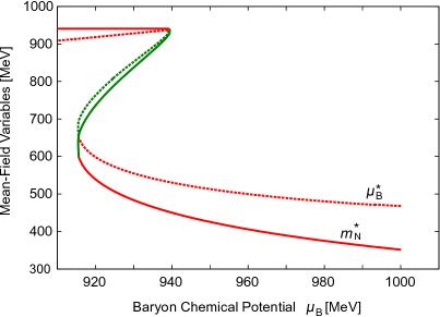
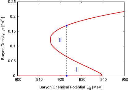
Figure 6: (Left) Mean-field variables as functions of $\mu_{\text{B}}$. There is a first-order phase transition from the low-density state in which the nucleon mass is the bare one to the high-density state in which the in-medium nucleon mass drops to almost a half. The green curves represent the unstable solutions of the gap equation. (Right) Baryon density as a function of the chemical potential. The first-order phase transition occurs so that the area in the region I is equal to that in the region II.

Two coupling constants are chosen so as to satisfy the following saturation properties of nuclear matter, that is,

$$\frac{\varepsilon}{\rho}\biggr{|}_{\rho=\rho_{0}}=m_{\text{N}}-16.3\;\text{MeV}\;,\qquad\frac{d(\varepsilon/\rho)}{d\rho}\biggr{|}_{\rho=\rho_{0}}=0\;.$$ (51)

We make a remark that the latter is understood as a stability condition for nuclear droplet. In fact, this density derivative at $T=0$ leads to $d(\varepsilon/\rho)/d\rho=\mu_{\text{B}}/\rho-\varepsilon/\rho^{2}=p/\rho^{2}=0$. We note that this $p$ is a pressure difference between the nuclear droplet and the empty vacuum. When we discuss the liquid-gas phase transition of quark matter, we will come back to this point. A set of parameters consistent with the nuclear matter properties is [89],

$$m_{\text{N}}=939\;\text{MeV}\;,\quad m_{\sigma}=550\;\text{MeV}\;,\quad m_{\omega}=783\;\text{MeV}\;,\quad g_{s}=10.3\;,\quad g_{\omega}=12.7\;.$$ (52)

The behavior of the in-medium mass $m_{\text{N}}^{\ast}$ is plotted in the left panel of Fig. 6 together with the effective chemical potential $\mu_{\text{B}}^{\ast}$. It is clear from Fig. 6 that there is a first-order liquid-gas phase transition of nuclear matter (or the liquid-vacuum phase transition, strictly speaking). The nuclear matter should exhibit a first-order phase transition at $\mu_{\text{B}}=m_{\text{N}}-B/A\simeq 923\;\text{MeV}$. In thermodynamics, equivalently, we can find this critical value of $\mu_{\text{B}}$ from the condition that the thermodynamic potential $\Omega$ becomes balanced in two states. In view of the curve of $\rho(\mu_{\text{B}})$ in the right panel of Fig. 6 the phase transition point is determined so that the area in the region I is equal to that in the region II.  This can be understood from $\Delta\Omega({\mu_{\text{B}}}_{c})=\Omega({\mu_{\text{B}}}_{c})-\Omega({\mu_{\text{B}}}_{c})=-\oint_{{\mu_{\text{B}}}_{c}}^{{\mu_{\text{B}}}_{c}}\rho(\mu)d\mu=0$ along the path from the lower dot to the upper dot in the right panel of Fig. 6. Such a way to find ${\mu_{\text{B}}}_{c}$ is reminiscent of the Maxwell construction for $p$ and $V$.

The left panel of Fig. 7 is the saturation curve of the energy per nucleon as a function of the baryon density $\rho$. Obviously the saturation point and the binding energy agree with the values in Eq. (51) as a result of the fit. In this simplest setup, however, the compressibility cannot be reproduced well, and a potential term $V(\sigma,\omega)$ should be added in Eq. (45) [90], which we will not discuss, for we are mostly interested in the qualitative aspects of the phase structure.

3.1.2 Liquid-gas phase transition of symmetric nuclear matter

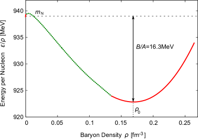
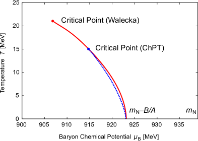
Figure 7: (Left) The saturation curve of the energy per nucleon as a function of the baryon density $\rho$. The global minimum is located at the saturation density. The dotted curve represents the unstable solution of the gap equation. (Right) First-order phase boundary and the critical point in the Walecka model and in the chiral perturbation theory in the three-loop order [91].

The existence of the first-order phase transition is an inevitable consequence from the saturation properties of symmetric nuclear matter. This world as it is, in other words, embodies the mixed state, and in general, a self-bound system of fermionic particles should have a first-order phase transition.

Differently than the second-order phase transition governed by the global symmetry and its spontaneous breaking, the first-order phase transition in nuclear matter does not change the symmetry pattern at all. Because two states before and after the transition have a different density as seen clearly in the right panel of Fig. 6, one can regard this type of the transition as associated with the density. Then, typically, the dilute phase corresponds to a gaseous state and the dense phase corresponds to a liquid state, and nuclear matter hence results in the liquid-gas phase transition. Right at the first-order phase transition a mixed state should be formed, during which the gas and the liquid parts can coexist in space. The most optimal spatial shape should emerge from the competition between the Coulomb energy and the surface energy (see Ref. [92] and references therein), and the resulting peculiar shapes are referred to as various “pasta” phases.

To fit the saturation properties the Walecka model was solved at $T=0$, and it is straightforward to extend such model calculations to the finite-$T$ situation. We have already written the gap equations (47) down with the matter terms. Then, solving them numerically, we can make a prediction for the first-order boundary elongated toward $T\neq 0$. In the Walecka model meson fluctuations are totally neglected, and thus, we should not apply this model to the analysis at high $T$ where abundant pions are thermally excited. As noticed in the numerical results in Fig. 7, the terminal point of the first-order phase boundary (i.e. the critical point) lies around $T\sim 20\;\text{MeV}$, which is small enough to justify our neglecting pion fluctuations.

The phase boundary tends to bend toward smaller chemical potential with increasing temperature, which can be understood from the Clausius-Clapeyron relation [93]. On the first-order phase transition the thermodynamic potential should be balanced between two phases. If we move along the phase boundary from $T$ and $\mu_{\text{B}}$ by infinitesimal $dT$ and $d\mu_{\text{B}}$, the thermodynamic potentials, $\Omega_{\text{dilute}}$ in a dilute state and $\Omega_{\text{dense}}$ in a dense state should remain equal, which immediately leads to

$$\frac{\partial\Omega_{\text{dilute}}}{\partial T}dT+\frac{\partial\Omega_{\text{dilute}}}{\partial\mu_{\text{B}}}d\mu_{\text{B}}=\frac{\partial\Omega_{\text{dense}}}{\partial T}dT+\frac{\partial\Omega_{\text{dense}}}{\partial\mu_{\text{B}}}d\mu_{\text{B}}\quad\Rightarrow\quad\frac{dT}{d\mu_{\text{B}}}=-\frac{\Delta\rho}{\Delta s}\;,$$ (53)

where $\Delta\rho=\rho_{\text{dense}}-\rho_{\text{dilute}}$ is the density difference and $\Delta s=s_{\text{dense}}-s_{\text{dilute}}$ is the entropy difference. The slope $dT/d\mu_{\text{B}}$ is negative in Fig. 7 and this implies that $\Delta\rho$ and $\Delta s$ should have the same sign. In most cases, indeed, the entropy density becomes greater in the dense state than in the dilute state, which means $\Delta\rho/\Delta s>0$.

From the theoretical point of view the underlying mechanism in quark matter to produce a first-order phase transition is exactly the same as that in the Walecka model we elucidated here. In the case of quark matter, however, there is no strong support for the existence of the first-order phase transition.

3.2 Chiral perturbation theory

One of the most advanced methods to deal with nuclear matter in a relativistic framework is the chiral perturbation theory. We have already introduced a Lagrangian (32) that describes low-energy chiral dynamics. It was necessary to utilize the linear sigma model because $\sigma$ can be a soft mode at chiral restoration. At low temperatures, however, chiral symmetry is significantly broken, and the low-energy dynamics is completely ruled by the light NG bosons. Hence, it should be the most appropriate to formulate an effective theory in terms of the NG bosons only, which is obtainable by integrating $\sigma$ out from the linear sigma model. In such a way, one can come by a non-linear representation of the low-energy effective theory. Actually, thanks to the low-energy theorems, one can adopt any representation only to get the same physics results (Haag theorem) [94], which provides us with a systematic and model-independent tool to disclose the properties of hadronic matter.

3.2.1 Effective Lagrangian and the power counting

In the vacuum we do not have to consider the scalar particles because they are much heavier than the NG bosons. Then, as seen in Eq. (33), the theory is defined as a function of $\boldsymbol{\tau}\cdot\boldsymbol{\pi}$ where $\boldsymbol{\tau}$ is the Pauli matrices in isospin space in the $N_{\text{f}}=2$ case. It is the most useful choice to employ a representation in terms of unitary matrix,

$$U=e^{i\boldsymbol{\tau}\cdot\boldsymbol{\pi}/f_{\pi}}\;,\qquad U\;\to\;L^{\dagger}\,U\,R\;,$$ (54)

having the same transformation property as $M$ with the $\sigma$ meson dropped off. The chiral-symmetric Lagrangian density is to be expanded in terms of $U$ and derivatives; the lowest-order is

$$\mathcal{L}_{\pi}^{(2)}=\frac{f_{\pi}^{2}}{4}\text{tr}(D_{\mu}UD^{\mu}U^{\dagger})+\frac{f_{\pi}^{2}}{4}\text{tr}(\chi U^{\dagger}+U\chi^{\dagger})\;,$$ (55)

with two derivatives and and one symmetry breaking term. The parameter in the latter term is $\chi=2B_{0}(s+ip)$ where $s$ is the quark mass matrix. Using $B_{0}$ one can express the chiral condensate as $\langle\bar{q}q\rangle=-f_{\pi}^{2}B_{0}$ and the pion mass as $m_{\pi}^{2}=(m_{u}+m_{d})B_{0}$ which is consistent with the Gell-Mann-Oakes-Renner relation (24). The covariant derivative is defined as $D_{\mu}U=\partial_{\mu}U+i\ell_{\mu}U-iUr_{\mu}$ that transforms as $D_{\mu}U\;\to\;L^{\dagger}(x)(D_{\mu}U)R(x)$ with properly defined $\ell_{\mu}$ and $r_{\mu}$ for local chiral rotations $L(x)$ and $R(x)$ as in the gauge theory.

The chiral effective Lagrangian (55) can be regarded as the lowest-order $\mathcal{O}(p^{2})$ contribution in the expansion with respect to pion momentum scale $p$ as compared to the typical chiral scale $\Lambda_{\chi}=4\pi f_{\pi}\sim 1\;\text{GeV}$. Then, the pion mass $m_{\pi}$ is $\mathcal{O}(p)$ and then $\chi\propto m_{\pi}^{2}$ is $\mathcal{O}(p^{2})$. We can perform the theoretical calculation for physical observables up to $\mathcal{O}(p^{2})$ using this Lagrangian (55) at the tree-level. To go to the next order of $\mathcal{O}(p^{4})$, one should include one-loop diagrams from $\mathcal{L}_{\pi}^{(2)}$ together with the tree-level contributions from $\mathcal{L}_{\pi}^{(4)}$ at $\mathcal{O}(p^{4})$. In the $\mathrm{SU}(N_{\text{f}}=3)$ case there are 10 independent terms (including $\chi$, $\ell_{\mu}$, $r_{\mu}$) and 10 low-energy constants are required at $\mathcal{O}(p^{4})$. In the $\mathrm{SU}(2)$ case there are less parameters. These constants are fixed to fit with the experimental data of the meson masses, $\pi$-$\pi$ scattering, rare pion decays, $K_{\ell 4}$ decay, $f_{K}/f_{\pi}$, etc, and then one can carry theoretical predictions out. This systematic program of the low-energy expansion of the effective theory of QCD in terms of the NG bosons is called the chiral perturbation theory (ChPT).

Let us consider how to apply the ChPT to figure out the behavior of the chiral condensate at finite temperature and density. Because the operator $\bar{\psi}\psi$ and the quark mass $m_{\text{q}}$ are conjugate to each other, the chiral condensate $\langle\bar{\psi}\psi\rangle$ is derived from the derivative of the thermodynamic potential $\Omega$ with respect to $m_{\text{q}}$, that is, $\langle\bar{\psi}\psi\rangle=-\partial\Omega/\partial m_{\text{q}}$. Thanks to the GOR relation (24), it is a straightforward procedure to convert the $m_{\text{q}}$-derivative to that in terms of the pion mass squared $m_{\pi}^{2}$. Then, in a medium at finite $T$ and density $\rho$, the deviation of the in-medium chiral condensate from the vacuum value $\langle\bar{\psi}\psi\rangle_{0}$ can be expressed as

$$\frac{\langle\bar{\psi}\psi\rangle_{T,\rho}}{\langle\bar{\psi}\psi\rangle_{0}}=1-f_{\pi}^{-2}\biggl{(}\frac{\partial\Omega}{\partial m_{\pi}^{2}}+\frac{\sigma_{\pi\text{N}}}{m_{\pi}^{2}}\frac{\partial\Omega}{\partial m_{\text{N}}}\biggr{)}\;,$$ (56)

where the second contribution has the nuclear sigma term that is defined and estimated as [95, 96],

$$\sigma_{\pi\text{N}}\equiv m_{\text{q}}\frac{\partial m_{\text{N}}}{\partial m_{\text{q}}}\simeq 45\;\text{MeV}\;.$$ (57)

The lowest-order correction originates from contributions induced by $T$ from the free pion gas and $\rho$ from the free nucleon gas. If the pion mass can be negligible (i.e. $m_{\pi}\simeq 0$) and $\rho$ is sufficiently small enough to approximate the scalar density $\rho_{\text{s}}=-\partial\Omega/\partial m_{\text{N}}$ with the density $\rho$, the analytical integration is possible, leading to [97, 98],

$$\frac{\langle\bar{\psi}\psi\rangle_{T,\rho}}{\langle\bar{\psi}\psi\rangle_{0}}=1-\frac{T^{2}}{8f_{\pi}^{2}}-\frac{\sigma_{\pi\text{N}}}{m_{\pi}^{2}f_{\pi}^{2}}\,\rho+\mathcal{O}(T^{4},\rho^{2})\;,$$ (58)

at the lowest order in the linear density approximation. The finite-$m_{\pi}$ correction is not really negligible, in fact, and the expansion breaks down around $T\sim 150\;\text{MeV}$ due to the neglected excitations of other mesonic states. Because the $\sigma$ meson decouples from the dynamics, one has no chance to describe the chiral phase transition using the non-linear representation. Nevertheless, it would be suggestive to see explicitly where the chiral condensate vanishes with increasing $T$ and $\rho$ according to the lowest-order expression (58). The results are depicted in the left panel of Fig. 8. It seems that the chiral condensate disappears to draw a sort of the phase boundary on the $T$-$\rho$ plane, though the approximation in Eq. (58) breaks down there. Even though we cannot reach the chiral phase transition in the ChPT, such in-medium reduction of the chiral condensate or $f_{\pi}$ can be an experimental measure for the partial restoration of chiral symmetry [99] (see also Eq. (66)).

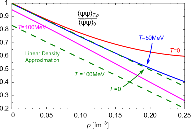
Figure 8: (Left) Chiral condensate at finite $T$ and $\rho$ in the limit of the free pion gas and the linear density approximation given in Eq. (58). (Right) Chiral condensate calculated in the NLO three-loop order. Figure adapted from Ref. [100] and the linear density approximation results (dashed lines) are overlaid for reference.

3.2.2 Application to nuclear matter

It is necessary to take account of the heavy baryonic degrees of freedom into the dynamics at high density. The fermion part is expressed by the Lagrangian, $\mathcal{L}=\bar{\psi}\bigl{[}i\hbox to5.30904pt{\hbox to0.0pt{\hbox to5.30904pt{\hss/\hss}\hss}\hbox{$\partial$}}-g(\sigma-i\boldsymbol{\tau}\cdot\boldsymbol{\pi})\bigr{]}\psi$, which is converted into the non-linear representation after dropping the scalar field. The usual procedure to write the baryon theory down is to perform the field redefinition as

$$\xi=e^{i\boldsymbol{\tau}\cdot\boldsymbol{\pi}/2f_{\pi}}\;,\qquad N_{\text{L}}=\xi^{\dagger}\psi_{\text{L}}\;,\qquad N_{\text{R}}=\xi\psi_{\text{R}}\;,\qquad U=\xi\xi\;.$$ (59)

Then the fermionic Lagrangian is translated into the form similar to the gauge theory, $\mathcal{L}=\bar{N}(i\hbox to8.55695pt{\hbox to0.0pt{\hbox to8.55695pt{\hss/\hss}\hss}\hbox{$D$}}-\hbox to7.50002pt{\hbox to0.0pt{\hbox to7.50002pt{\hss/\hss}\hss}\hbox{$A$}}\gamma_{5}-\boldsymbol{m})N$, with $D_{\mu}=\partial_{\mu}+iV_{\mu}$ and the vector and the axial-vector fields,

$$V_{\mu}=-\frac{i}{2}(\xi^{\dagger}\partial_{\mu}\xi+\xi\partial_{\mu}\xi^{\dagger})\;,\qquad A_{\mu}=-\frac{i}{2}(\xi^{\dagger}\partial_{\mu}\xi-\xi\partial_{\mu}\xi^{\dagger})\;.$$ (60)

Including the renormalization constants that change the axial-vector coupling from unity to $g_{A}\simeq 1.26$, the nucleon effective Lagrangian is expanded in terms of the pion fields up to the quadratic order as

$$\mathcal{L}_{\text{N}}=\bar{N}(i\hbox to5.30904pt{\hbox to0.0pt{\hbox to5.30904pt{\hss/\hss}\hss}\hbox{$\partial$}}-m_{\text{N}})N+\frac{g_{A}}{f_{\pi}}\bar{N}\gamma^{\mu}\gamma_{5}\frac{\boldsymbol{\tau}}{2}N\cdot\partial_{\mu}\boldsymbol{\pi}-\frac{1}{4f_{\pi}^{2}}\bar{N}\gamma^{\mu}\boldsymbol{\tau}\cdot\boldsymbol{\pi}\times\partial_{\mu}\boldsymbol{\pi}N+\frac{\sigma_{\pi\text{N}}}{2f_{\pi}^{2}}\boldsymbol{\pi}^{2}\bar{N}N$$ (61)

with the pseudo-vector $\pi NN$-vertex and the Tomozawa-Weinberg $\pi\pi NN$-contact vertex. With these interaction vertices the thermodynamics and the chiral condensate are derived; the next-to-leading-order (NLO) results are calculated and shown in the right panel of Fig. 8 adapted from Ref. [100]. The linear density approximation comes to work fine for $T\gtrsim 50\;\text{MeV}$, while the $T$-dependence at NLO shows a significant deviation from Eq. (58).

From the point of view of the systematic expansion with respect to the energy scale, it is not straightforward to formulate perturbative expansions involving baryons with the consistent power counting. A new scale, i.e. the nucleon mass $m_{\text{N}}$, is not small as compared to the chiral symmetry breaking scale $\Lambda_{\chi}$ and appears in higher loops that contribute to lower order. Thus, the apparent one-to-one correspondence between the loop and the derivative expansions is, at first glance, lost. Yet, within the fully relativistic framework one can retrieve the consistent power counting for multi-loop diagrams using appropriate renormalization conditions [101, 102]. Another resolution to avoid this drawback is to adopt a heavy baryon reduction yielding the non-relativistic limit of the original theory, that is, the heavy baryon chiral perturbation theory (HBChPT) where the power counting is restored [103]. We write the nucleon momentum as

$$p^{\mu}=m_{\text{N}}v^{\mu}+k^{\mu}\;,$$ (62)

where $v^{\mu}$ is the four-velocity with $v^{2}=1$ and $k^{\mu}$ is the residual momentum of order $\Lambda_{\text{QCD}}$, so that one can perform the derivative expansion systematically in energy range below $\Lambda_{\chi}$. The Lagrangian density is written in terms of the nucleon field $B$ carrying $v^{\mu}$ which is related to the original field $N$ via

$$B(x)=\exp\bigl{(}im_{\text{N}}v\cdot x\bigr{)}\,N(x)\;.$$ (63)

With this the nucleon part of the Lagrangian density becomes

$$\mathcal{L}_{\text{N}}=\bar{N}\bigl{(}i\gamma^{\mu}\partial_{\mu}-m_{\text{N}}\bigr{)}N=\bar{B}\,iv^{\mu}\partial_{\mu}B\;.$$ (64)

Therefore no hard scale appears in the theory. Higher-order terms are arranged in powers of $k^{\mu}/\Lambda_{\chi}$ and $k^{\mu}/m_{\text{N}}$. Loop calculations in the HBChPT framework are simpler as compared to the relativistic treatment and the HBChPT has been applied to a broad range of the nuclear physics problems. For reviews, see Refs. [104, 105, 106].

In the nuclear medium the methodology of chiral effective field theory can also be formulated. The in-medium ChPT Lagrangian is derived from the generating functional after integrating the nucleon fields out but keeping the particle-hole part of the fermion determinant. The in-medium pion decay constants,

$$\langle N|J_{\text{A}}^{0}(x)|\pi(q)\rangle=iq^{0}\,f_{\pi}^{t}\,e^{iqx}\;,\qquad\langle N|J_{\text{A}}^{i}(x)|\pi(q)\rangle=iq^{i}\,f_{\pi}^{s}\,e^{iqx}\;,$$ (65)

are found at one-loop order in symmetric nuclear matter as [107]

$$f_{\pi}^{t}(\rho)=f_{\pi}\left[1-\frac{\rho}{\rho_{0}}(0.26\pm 0.04)\right]\;,\qquad f_{\pi}^{s}(\rho)=f_{\pi}\left[1-\frac{\rho}{\rho_{0}}(1.23\pm 0.07)\right]\;.$$ (66)

A model-independent analysis valid at low density leads to a scaling relation between $f_{\pi}^{t}$ and the in-medium quark condensate [108], with which one sees that the condensate decreases in nuclear matter, indicating partial restoration of chiral symmetry (see Ref. [109] for a review).

3.3 Mesons, baryons, and exotica

From the ChPT one can calculate how the chiral condensate decreases. If the chiral condensate significantly drops, then, it should have sizable influences on the hadron spectra such as the nucleon mass. Indeed we have already elucidated that the in-medium effective mass in the Walecka model is different largely from the bare value. The question is, then, how chiral symmetry becomes manifest for the hadronic degrees of freedom if (partial) chiral restoration occurs in dense matter.

3.3.1 Mended symmetry

In general a large variety of representations are possible for composite states made from quarks that belong to the fundamental representation. When chiral symmetry $G$ were not spontaneously broken down into $H$, the physical states would be classified by irreducible representations of $G$. With broken chiral symmetry, the physical states belong no longer to those irreducible representations, but instead are superposition of all the possible representations. The physical state $|\alpha\rangle$ is expressed in a series of a complete set of states $|J\rangle$ characterized by good quantum numbers $J$;

$$|\alpha\rangle=\sum_{J}c_{J}|J\rangle\;.$$ (67)

The coefficients $c_{J}$ contain information about the broken chiral symmetry. The state $|\alpha\rangle$ can further be constrained by applying the large-$N_{\text{c}}$ approximation (see Sec. 3.5 also) as well as current algebraic relations [110, 111]. The states for the low-lying excitations with zero helicity are classified by a limited number of the irreducible representations and form a closed algebra which is referred to as mended symmetries.

As shown in Ref. [110], assuming that the Adler-Weisberger sum rules for the scattering process, $\pi_{a}+\alpha(\lambda)\to\pi_{b}+\beta(\lambda^{\prime})$ for helicities $\lambda$ and $\lambda^{\prime}$, can be saturated with narrow one-particle states, the set of the sum rules is put into the Lie-algebraic form,

$$\left[X_{a},X_{b}\right]=if_{abc}T_{c}\;,$$ (68)

where $f_{abc}$ is the structure constant, $T_{c}$ is the generator of the $\mathrm{SU}(N_{\text{f}})_{\text{V}}$ group that satisfies

$$\left[T_{a},T_{b}\right]=if_{abc}T_{c}\;,$$ (69)

and $X_{a}$ is the axial-vector coupling matrix defined from the matrix elements at zero invariant momentum transfer of the axial-vector current between states with collinear momenta via

$$\langle\vec{q}\lambda^{\prime}\beta|(J_{\text{A}a}^{0}+J_{\text{A}a}^{3})|\vec{p}\lambda\alpha\rangle=(2\pi)^{3}2p^{+}\delta^{3}(\vec{p}-\vec{q})\delta_{\lambda^{\prime}\lambda}\left[X_{a}(\lambda)\right]_{\beta\alpha}\;.$$ (70)

Thus, from this definition, some non-trivial calculations lead us to the following commutation relation,

$$\left[T_{a},X_{b}\right]=if_{abc}X_{c}\;.$$ (71)

Putting together, Eqs. (68), (69), and (71) close the algebra and one sees that the $X_{a}$ together with the unbroken $\mathrm{SU}(N_{\text{f}})_{\text{V}}$ generators $T_{c}$ satisfies the commutation relations of the Lie algebra of the broken symmetry group $G$.

In the broken phase the $X_{a}$ is not symmetry generators. In fact, it does not commute with mass-squared matrix $m^{2}$. We note that $m^{2}$ here refers to the general hadron masses and is not necessarily vanishing in the chiral symmetric phase. The non-commutativity which follows from Eq. (68) along with the Jacobi identity defines $m_{4}^{2}$, that is, the chiral-symmetry breaking part of $m^{2}$ as

$$\left[X_{b},\left[m^{2},X_{a}\right]\right]=-m_{4}^{2}\delta_{ab}\;.$$ (72)

In the $N_{\text{f}}=2$ case, for example, $m_{4}$ transforms as the fourth component of a chiral four-vector (like the $\sigma$ meson). This tells us that the mass matrix is a sum of a chiral-singlet $m_{0}^{2}$ that satisfies $[X_{a},m_{0}^{2}]=0$ and a non-singlet $m_{4}^{2}$, i.e.

$$m^{2}=m_{0}^{2}+m_{4}^{2}\;.$$ (73)

When $m_{4}^{2}$ vanishes, i.e. chiral symmetry is restored, $X_{a}$ becomes true symmetry generators, so that $X_{a}$ commutes with $m^{2}$ and hadrons form degenerate multiplets filling out a complete set of representations of $G$.

In the chiral broken phase the algebraic representations of $X_{a}$ do not always coincide with the mass eigenstates as accounted for by $\left[X_{a},m^{2}\right]\neq 0$. In general, there, physical particle states are expressed as a sum of all possible elements of various representations of the Lie algebra composed of $X_{a}$ and $T_{c}$. The $X_{a}$ is therefore entirely determined by the mixing angles which define the coefficients of the representations in the sum. Let the physical states of the low-lying $\lambda=0$ mesons, the scalar $\sigma$, pseudo-scalar $\pi$, vector $\rho$ and axial-vector $a_{1}$ mesons, be in the following admixture of the chiral representations [110, 112],

$$\begin{split}|\pi\rangle&=|\left(N_{\text{f}},N_{\text{f}}^{\ast}\right)\oplus\left(N_{\text{f}}^{\ast},N_{\text{f}}\right)\rangle\sin\theta{}+|\left(N_{\text{f}}^{2}\!-\!1,1\right)\oplus\left(1,N_{\text{f}}^{2}\!-\!1\right)\rangle\cos\theta\;,\\ |a_{1}(\lambda=0)\rangle&=|\left(N_{\text{f}},N_{\text{f}}^{\ast}\right)\oplus\left(N_{\text{f}}^{\ast},N_{\text{f}}\right)\rangle\cos\theta{}-|\left(N_{\text{f}}^{2}\!-\!1,1\right)\oplus\left(1,N_{\text{f}}^{2}\!-\!1\right)\rangle\sin\theta\;,\\ |\sigma\rangle&=|\left(N_{\text{f}},N_{\text{f}}^{\ast}\right)\oplus\left(N_{\text{f}}^{\ast},N_{\text{f}}\right)\rangle\;,\\ |\rho(\lambda=0)\rangle&=|\left(N_{\text{f}}^{2}\!-\!1,1\right)\oplus\left(1,N_{\text{f}}^{2}\!-\!1\right)\rangle\;.\end{split}$$ (74)

This quartet structure based on the chiral algebraic sum rules is known as a notion of mended symmetry [111]. This leads to the decay widths as functions of the mixing angle $\theta$ and masses as well as $f_{\pi}$. The experimental rate for $\rho\to\pi+\pi$ and the pion decay constant $f_{\pi}$ give approximately $\theta\approx 45^{\circ}$ and one then finds

$$m_{\rho}\approx m_{\sigma}\;,\qquad m_{a_{1}}^{2}\approx 2m_{\rho}^{2}\;,$$ (75)

indicating that the above algebraic consideration indeed yields the reasonable order of magnitude for the masses.

Apparently, those helicity-zero mesons as well as the pion all become massless at a second-order phase transition where $m_{\sigma}$ becomes vanishing [111]. When an external parameter, such as $T$ and $\rho$, drives a system from broken to unbroken phase, the mixing angle is in general supposed to have some intrinsic dependence on the external parameter. Such medium evolution of the mixing angle needs to be pinned down so that some signals of the chiral phase transition in hadronic quantities would be revealed.

3.3.2 The problem of mass

In introducing baryon fields, there are two alternative ways of assigning chirality to the nucleons. Let us consider a pair of chiral partners, $\psi_{1}$ and $\psi_{2}$, that realizes chiral $\mathrm{SU}(2)_{\text{L}}\times\mathrm{SU}(2)_{\text{R}}$. One is,

$$\begin{split}\text{(Standard Assignment)}\qquad&\psi_{1\text{L}}\to L\psi_{1\text{L}}\;,\qquad\psi_{1\text{R}}\to R\psi_{1\text{R}}\;,\\ &\psi_{2\text{L}}\to L\psi_{2\text{L}}\;,\qquad\psi_{2\text{R}}\to R\psi_{2\text{R}}\;,\end{split}$$ (76)

which is anchored on the standard chiral symmetry structure where the entire constituent quark or nucleon mass (in the chiral limit) is generated via spontaneous chiral symmetry breaking. The other is [113],

$$\begin{split}\text{(Mirror Assignment)}\qquad&\psi_{1\text{L}}\to L\psi_{1\text{L}}\;,\qquad\psi_{1\text{R}}\to R\psi_{1\text{R}}\;,\\ &\psi_{2\text{L}}\to R\psi_{2\text{L}}\;,\qquad\psi_{2\text{R}}\to L\psi_{2\text{R}}\;,\end{split}$$ (77)

which allows for a chiral invariant mass term,

$$\mathcal{L}_{m}=m_{0}\bigl{(}\bar{\psi}_{2\text{L}}\psi_{1\text{R}}-\bar{\psi}_{2\text{R}}\psi_{1\text{L}}-\bar{\psi}_{1\text{L}}\psi_{2\text{R}}+\bar{\psi}_{1\text{R}}\psi_{2\text{L}}\bigr{)}\;,$$ (78)

with which $m_{0}$ remains non-zero at chiral restoration. One should notice that the left- and right-handedness of a fermion is the representation of the Lorentz group, whereas chiral symmetry is entirely associated with the internal symmetry. Therefore those must be in general dealt with independently, which enables us to adopt the above non-standard chiral rotation. In other words, the mirror assignment is possible since the nucleon is not an elementary particle but a composite state made from quarks.

A part of the nucleon mass, $m_{0}$, must arise from a mechanism that is not associated with spontaneous chiral symmetry breaking. Various observables both in the vacuum such as baryon decays [114] and pion-nucleon scattering [115, 116] and in a medium such as nuclear matter properties [117, 118, 119, 120] and the thermal gluon condensate [121] have been explored based on chiral Lagrangian approaches with mirror baryons. The analysis tells us that an $m_{0}$ of a few hundred MeV cannot be ruled out. In the non-linear realization of chiral symmetry only the properties coming from the vectorial transformation are remained [122], and therefore the standard and mirror assignments cannot be distinguished. Even if indistinguishable in matter-free space, they are expected to start showing their differences due to the remaining $m_{0}$ as one approaches the chiral restoration point.

What is the origin of such a mass $m_{0}$? Recall that the emergence of $\Lambda_{\text{QCD}}$ is signaling the breaking of conformal invariance, i.e. the trace anomaly, of QCD in the chiral limit where the theory has no dimensionful parameters. Spontaneous chiral symmetry breaking, which gives rise to a nucleon mass, and the trace anomaly are intimately linked to each other [123] and dynamical scales in hadronic systems are then considered to originate from them. Hence, the origin of $m_{0}$ can be attributed to the non-vanishing gluon condensate in chiral symmetric phase [121] (see also discussions in Sec. 3.3.3).

This is reminiscent of Weinberg’s chiral-singlet mass in Eq. (73). The chiral representation mixing (74) would be expected to be resolved when chiral symmetry is restored in such a way that the $\pi$ and $\sigma$ mesons form a degenerate multiplet as chiral partners, as presumed from the argument of the $\mathrm{O}(4)$-universality class in $N_{\text{f}}=2$ QCD.  This is in fact realized when the mixing goes like $\cos\theta\to 0$ and with which the $\pi$ and $\sigma$ belong to the same representation $|(N_{\text{f}},N_{\text{f}}^{\ast})\oplus(N_{\text{f}}^{\ast},N_{\text{f}})\rangle$ and being massless protected by the NG theorem, whereas this is not the case for the $\rho$ and $a_{1}$ mesons being degenerate in the same representation at chiral restoration and in general having a non-vanishing common mass. It is also possible that those lowest-lying mesons form a quartet being all the mesons massless when the mixing remains unresolved as demonstrated using the mended symmetry notion in Ref. [111] where $m_{\rho}=m_{\sigma}$ is predicted. Or even with a resolving mixing, if there are some mechanisms that the $\rho$ and $a_{1}$ mesons become massless, the massless quartet can be well accommodated to the requirement of chiral restoration, such as in the context of the Brown-Rho (BR) scaling [124], an analysis of RG flows within a class of chiral effective field theory [125, 126] and of the non-linear sigma model implementing the trace anomaly [121].

Yet, massive vector bosons with no mixing at chiral restoration are not prohibited by symmetries. The mixing angle can be in general a function of temperature and density and therefore would develop in a hot/dense medium. Even if the mixing is preferred being $m_{\rho}=m_{\sigma}$ in matter-free space, it might evolve so that $\cos\theta\to 0$, not optionized in Ref. [111], namely $m_{\pi}=m_{\sigma}=0$ and $m_{\rho}=m_{a_{1}}\neq 0$ can be allowed.

3.3.3 Thermodynamics of dilatons

The trace anomaly is implemented in a chiral Lagrangian by introducing a dilaton (or scalar glueball) field $\chi$ representing the gluon condensate $\langle G_{\mu\nu}G^{\mu\nu}\rangle$ [127, 128]. Requiring that the dilatation current associated with scale transformation is saturated by a condensed dilation field leads to the potential,

$$V_{\chi}=\frac{B}{4}\biggl{(}\frac{\chi}{\chi_{0}}\biggr{)}^{4}\biggl{[}\ln\biggl{(}\frac{\chi}{\chi_{0}}\biggr{)}^{4}-1\biggr{]}\;.$$ (79)

The two parameters, i.e. the bag constant $B$ and a scale parameter $\chi_{0}$, are fixed from the vacuum energy density $\mathcal{E}=\frac{1}{4}B$ and the glueball mass $M_{\chi}=2\sqrt{B}/\chi_{0}$. Effective Lagrangians are written so that they possess chiral and scale invariance, mimicking dynamical breaking of those symmetries of QCD in low energies.

In relativistic nuclear physics, a scalar boson plays an essential role as a mediator of the medium-range $NN$ interaction as we discussed using the Walecka model in Sec. 3.1. The important lesson from the model studies is that this scalar degree of freedom cannot be identified with the scalar meson that appears as the chiral partner of the NG boson in a linear sigma model since otherwise no stable nuclear ground state is achieved and one cannot reproduce the basic saturation properties [129, 130]. This problem would be resolved in a non-linear representation as in the ChPT, or different chiral approaches have been introduced with modified interaction potentials among the chiral fields and the dilaton [130, 131, 132]. A non-linear chiral Lagrangian with a soft dilaton [133] is derived when a heavy component of the dilaton, responsible for the pure glueball dynamics, is integrated out [134].

Besides those approaches implementing the dilaton, a parity doublet model based on the mirror assignment can also be accommodated to the nuclear ground state [118]. The presence of a chiral invariant mass $m_{0}$ of the nucleons is essential there and a relatively large $m_{0}\sim 800\;\text{MeV}$ is favored in order to have the known nuclear matter properties. (This number becomes reduced substantially when a tetra-quark state is introduced and $m_{0}$ in nuclear matter results in $\sim 500\;\text{MeV}$ [120].)

It appears that $m_{0}$ plays a similar role to the dilaton in nuclear matter and thus a non-vanishing condensate of the dilaton field is a conceivable origin of $m_{0}$ [121, 116]. The scalar meson as the chiral partner of the pion generates only the mass difference of the nucleon parity doublers.

3.3.4 Four-quark condensate in a medium

Four-quark states were suggested as the lightest scalar mesons [135, 136] and this explains naturally the degenerate $a_{0}(980)$ and $f_{0}(980)$ states. How does the four-quark condensate evolve with temperature or density? The NG theorem by itself does not dictate a particular operator to fulfill a non-trivial commutation relation with the broken charge $Q_{\text{A}}$. Any operators $\mathcal{O}$ yielding non-commutativity to $Q_{\text{A}}$ guarantee spontaneous chiral symmetry breaking as discussed in Sec. 2.2.1. Besides $\mathcal{O}\sim\bar{\psi}t^{a}\psi$, some operators with higher dimensions such as a four-quark are possible.

In matter-free space the four-quark condensates are often evaluated assuming factorization,

$$\langle\bar{\psi}\bar{\psi}\psi\psi\rangle\simeq\langle\bar{\psi}\psi\rangle^{2}\;.$$ (80)

This indicates that the four-quark condensate seems to vanish at the chiral phase transition as $\langle\bar{\psi}\psi\rangle$. However, the factorized form (80) is justified in the large-$N_{\text{c}}$ limit only and not quite accurate in the real QCD case with $N_{\text{c}}=3$. Its validity in a hot/dense medium is even less justifiable.

Therefore, the issue is that when $\langle\bar{\psi}\psi\rangle$ vanishes, some four-quark operators (apart from the chiral singlet part) can condense so that it breaks chiral symmetry dynamically. Such a possibility has been considered at zero temperature and zero density in Refs. [137, 138], where a non-standard pattern of dynamical symmetry breaking was suggested. This pattern keeps the center of chiral group unbroken, i.e.

$$\mathrm{SU}(N_{\text{f}})_{\text{L}}\times\mathrm{SU}(N_{\text{f}})_{\text{R}}\to\mathrm{SU}(N_{\text{f}})_{\text{V}}\times\mathrm{Z}_{N_{\text{f}}}\;.$$ (81)

The discrete $\mathrm{Z}_{N_{\text{f}}}$ symmetry protects a theory from condensate of quark bilinears. Spontaneous symmetry breaking is driven by quartic condensates which are invariant under both $\mathrm{SU}(N_{\text{f}})_{\text{V}}$ and $\mathrm{Z}_{N_{\text{f}}}$ transformation. However, this pattern is strictly ruled out in QCD both at $T=0$ and $T\neq 0$ but $\mu_{\text{q}}=0$ since the axial-vector correlator becomes greater than the pseudo-scalar correlator then, which violates the QCD inequality [139]. This argument does not exclude the above unorthodox pattern in the presence of a dense medium because the QCD inequalities do not hold then. Several studies have been made, such as a similar dynamical breaking in an O(2) scalar model [140], constructing a Ginzburg-Landau free energy consistent with Eq. (81), and the exploration of its thermodynamic consequences [141].

3.4 Hidden local symmetries

The low-energy pion dynamics is well described by the non-linear sigma model on the manifold $G/H$ which is an effective Lagrangian in terms only of NG bosons transforming non-linearly under chiral rotation. The approach using the hidden local symmetry (HLS) [142, 143] is based on the fact that the non-linear sigma model is gauge equivalent to a model possessing $G_{\rm global}\times H_{\rm local}$ symmetry (see Ref. [144] for a review and references therein). As demonstrated explicitly in Refs. [145, 146], the dynamical generation of gauge bosons is a common phenomenon which appears in a variety of systems not restricted to particular models. Furthermore, one-loop quantization of the HLS theory based on the derivative expansion as made in the ordinary ChPT is established [144]. This enables us to evaluate loop effects systematically and thus the low-energy quantities with good precision come out combined with the RG analysis. Below, we briefly introduce the HLS approach and discuss several issues in strong coupling gauge theories.

3.4.1 $G_{\text{global}}\times H_{\text{local}}$ model

The Lagrangian is based on a $G_{\text{global}}\times H_{\text{local}}$ symmetry, where $G_{\text{global}}=[\mathrm{SU}(N_{\text{f}})_{\text{L}}\times\mathrm{SU}(N_{\text{f}})_{\text{R}}]_{\text{global}}$ is chiral symmetry and $H_{\text{local}}=[\mathrm{SU}(N_{\text{f}})_{\text{V}}]_{\text{local}}$ is the HLS.  The entire symmetry $G_{\text{global}}\times H_{\text{local}}$ is spontaneously broken to its diagonal subgroup $\mathrm{SU}(2)_{\text{V}}$. The basic quantities are the HLS gauge boson, $V_{\mu}$, and two matrix valued variables $\xi_{\text{L}}$, $\xi_{\text{R}}$, which are combined in an $N_{\text{f}}\times N_{\text{f}}$ special-unitary matrix $U=\xi_{\text{L}}^{\dagger}\xi_{\text{R}}$. There exists an ambiguity in the decomposition and this redundancy is identified with a local gauge transformation $H_{\text{local}}$. These variables are conventionally parameterized as

$$\xi_{\text{L,R}}(x)=e^{i\sigma(x)/{f_{\sigma}}}e^{\mp i\pi(x)/{f_{\pi}}}\,,$$ (82)

where $\pi=\pi^{a}T_{a}$ denotes the pseudo-scalar NG bosons associated with the spontaneous breaking of chiral symmetry, and $\sigma=\sigma^{a}T_{a}$ the NG bosons associated with the spontaneous breaking of $H_{\text{local}}$. The $\sigma$ is the longitudinal part of the vector meson and absorbed into the HLS gauge boson through the Higgs mechanism, so that the gauge boson acquires its mass. $f_{\pi}$ and $f_{\sigma}$ are the decay constants of the associated particles.

The main building blocks are $\hat{\alpha}_{\perp,\parallel}^{\mu}$ defined from the Maurer-Cartan 1-forms as

$$\hat{\alpha}_{\perp,\parallel}^{\mu}=\frac{1}{2i}\left(D^{\mu}\xi_{\text{R}}\cdot\xi_{\text{R}}^{\dagger}{}\mp D^{\mu}\xi_{\text{L}}\cdot\xi_{\text{L}}^{\dagger}\right)\;,$$ (83)

where the covariant derivatives of $\xi_{\text{L,R}}$ are given by

$$\begin{split}D_{\mu}\xi_{\text{\text{L}}}&=\partial_{\mu}\xi_{\text{L}}-iV_{\mu}\xi_{\text{L}}+i\xi_{\text{L}}{\mathcal{L}}_{\mu}\;,\\ D_{\mu}\xi_{\text{R}}&=\partial_{\mu}\xi_{\text{R}}-iV_{\mu}\xi_{\text{R}}+i\xi_{\text{R}}{\mathcal{R}}_{\mu}\end{split}$$ (84)

with ${\mathcal{L}}_{\mu}$ and ${\mathcal{R}}_{\mu}$ being the external gauge fields (weak bosons and photons) introduced by gauging $G_{\text{global}}$. The most general Lagrangian with lowest derivatives is given by [142]

$$\mathcal{L}=f_{\pi}^{2}\text{tr}\bigl{(}\hat{\alpha}_{\perp\mu}\hat{\alpha}_{\perp}^{\mu}\bigr{)}+f_{\sigma}^{2}\text{tr}\bigl{(}\hat{\alpha}_{\parallel\mu}\hat{\alpha}_{\parallel}^{\mu}\bigr{)}-\frac{1}{2g^{2}}\text{tr}\bigl{(}V_{\mu\nu}V^{\mu\nu}\bigr{)}\;,$$ (85)

where $g$ is the HLS gauge coupling and the field strength is $V_{\mu\nu}=\partial_{\mu}V_{\nu}-\partial_{\nu}V_{\mu}-i[V_{\mu},V_{\nu}]$. When the vector-meson kinetic term is ignored in low energy, the second term of the Lagrangian vanishes with the equation of motion of $V_{\mu}$ and the well-known non-linear sigma model on the coset space $G/H$ is derived. The leading-order Lagrangian contains two arbitrary parameters, $a=f_{\sigma}^{2}/f_{\pi}^{2}$ and $g$. For a particular choice $a=2$, the known phenomenological facts are successfully reproduced; universality of the vector meson coupling, the Kawarabayashi-Suzuki-Riazuddin-Fayyazudin (KSRF) relation, and vector meson dominance of the pion electromagnetic form factor [142].

There are other models of vector mesons introduced as the matter field, the anti-symmetric tensor field or in the massive Yang-Mills method. It is shown that they are equivalent to the gauge-fixed form of the HLS Lagrangian. For details, see e.g. Refs. [143, 147, 148, 144] and references therein.

3.4.2 Modeling strongly-coupled gauge theories

In principle one can enlarge the gauge group with more redundant variables. With such a generalized HLS (GHLS) [143, 149], the lowest-lying axial-vector mesons are embedded in a $G_{\text{global}}\times G_{\text{local}}$ model. Other higher-lying vector modes can also be incorporated systematically by introducing enlarged gauge symmetries. This idea is employed in so-called dimensional deconstruction which resembles the nearest neighbor interactions in condensed matter physics, constructed on a lattice [150, 151, 152]. The theory possesses gauge group which is a product of many numbers of the same gauge group. The interaction to matter fields is characterized by “theory space locality” [153] where the mixing of left and right chirality is generated only through gauge boson exchanges. Taking the continuum limit generates an extra dimension. Inspired by those studies, a dimensionally-deconstructed QCD was proposed [154]. The resultant five-dimensional Yang-Mills action is shown to reproduce some of known low-energy hadron properties.

The identical action implemented with the Chern-Simons action is obtained from the string theory based on the gauge/gravity duality (see Sec. 3.5.3 for the Sakai-Sugimoto model) [23, 155]. Performing the Kaluza-Klein mode expansion yields a four-dimensional action which contains the NG bosons and an infinite tower of vector and axial-vector mesons. When all the vector modes except the lowest-lying vector meson are integrated out, the $\mathcal{O}(p^{4})$ terms as well as the $\mathcal{O}(p^{2})$ terms of the HLS Lagrangian are generated [156]. The higher vector mesons are now accommodated in the $\mathcal{O}(p^{4})$ part.

Another type of duality of interest is the electric/magnetic duality in $\mathcal{N}=1$ supersymmetric Yang-Mills theory (i.e. Seiberg duality) [157]. For $\frac{3}{2}N_{\text{c}}<N_{\text{f}}<3N_{\text{c}}$ (conformal window), there exists a magnetic theory possessing the $\mathrm{SU}(N_{\text{f}}-N_{\text{c}})$ gauge symmetry which is dual to the original $\mathrm{SU}(N_{\text{c}})$ theory regarded as the electric theory. The two theories flow to the same IR fixed point and thus exhibit the identical low-energy dynamics. When $N_{\text{f}}$ decreases to $N_{\text{f}}=N_{\text{c}}$, the magnetic gauge symmetry induced at the composite level is spontaneously broken, which corresponds to the system with confinement and spontaneously broken chiral symmetry. It should be emphasized that the induced gauge symmetry has nothing to do with the original $\mathrm{SU}(N_{\text{c}})$ gauge symmetry, but it is rather analogous to the HLS [158].

Is the Seiberg duality realized in non-supersymmetric QCD under consideration? The answer is yes [159, 160]: The HLS theory is shown to exhibit chiral symmetry restoration by its own dynamics for large $N_{\text{f}}\sim 5\,(N_{\text{c}}/3)$, as in the $CP^{N-1}$ non-linear sigma model [143]. Therefore the $\mathrm{SU}(N_{\text{f}})$ HLS theory is considered to be the Higgsed magnetic theory dual to the electric theory, i.e. $\mathrm{SU}(N_{\text{c}})$ QCD.  Some consequences of this “QCD/HLS duality” in hadron physics are discussed e.g. in Refs. [160, 161].

Here we stress that the HLS theory appears as a potentially practical approach for various gauge theories in the strong coupling region. Obviously low-energy hadron physics, not only in matter-free space but also in a hot and/or dense medium, is a case of great interest. The HLS approach has been applied to QCD matter in a wide range of density and temperature. For reviews, see Refs. [162, 163, 164, 165, 166, 167] and references therein.

3.4.3 Chiral perturbation theory with HLS

Beyond the tree-level HLS results, loop effects are systematically evaluated at a given order of the derivative expansion as in the ordinary ChPT [168, 169]. The essential concept is the HLS gauge bosons treated as light. The chiral counting of the HLS gauge coupling is assigned of order $p$, which is equivalent to the order assignment by $m_{V}\sim\mathcal{O}(p)$ [170, 171]. The pionic coupling is derivative-type typically in non-linear realization. With the above counting, the vector mesons and their interaction can naturally be put in a perturbative treatment on the same footing with the NG bosons, yielding consistent counting rules. In real QCD the vector meson mass is not very small compared to the chiral symmetry breaking scale $\Lambda_{\chi}\sim 1\;\text{GeV}$. However, there exists a limit of large-$N_{\text{c}}$ in which the above expansion is certainly justified since

$$\frac{m_{V}^{2}}{\Lambda_{\chi}^{2}}\sim\frac{1}{N_{\text{c}}}\;.$$ (86)

Thus the entire procedure for the loop calculations should be regarded as an extrapolation from large-$N_{\text{c}}$ to $N_{\text{c}}=3$ QCD.  Indeed, combined with RG equations (RGEs), this works quite well and one sees the low-energy constants and the relevant quantities in the vector meson sector in good agreement with measurements [144].

Quadratic divergences that arise from the pion loops drive a system to chiral symmetry restoration (Wigner-Weyl realization). In the HLS theory this happens with the following conditions dictated by matching of the current correlation functions to those in the operator product expansion (OPE) [172]:

$$a\to 1\;,\qquad m_{V}\to 0\;.$$ (87)

The vector meson thus becomes massless toward chiral symmetry restoration where $f_{\pi}=0$, and falls into the same chiral multiplet together with the pion. Such somewhat non-standard realization called the vector manifestation (VM) is similar to the vector realization. The essential difference is that in the vector realization the NG boson pole residue $f_{\pi}$ remains non-vanishing whereas chiral symmetry is “unbroken”, i.e. $f_{\pi}\neq 0$, $\langle\bar{\psi}\psi\rangle=0$, therefore the system is not in the Wigner-Weyl phase (see Refs. [170, 171] for more details). Here one should be cautious of the fact that although the two realizations are formulated in the HLS framework, the theory contains a limited number of low-lying mesons, pseudo-scalar, and vector mesons, and in particular lack of a scalar particle near the restoration point is unsatisfactory from the point of view of building effective theories that describe the chiral phase transition. In fact, the two conditions in Eq. (87) correspond to the fixed points of the RGEs separately. Thus higher loops or other resonances would modify the RGEs and consequently parametric conditions of symmetry restoration. Nevertheless, the power of this effective field theory is that one can examine several scenarios allowed as phenomenological options, including the $m_{V}\neq 0$ case, within the single framework [173]. How the scalar mode emerges from non-linear sigma models is an issue [174, 121] and a naïve introduction of an elementary scalar field is known to cause the naturalness problem at loop level as in the Higgs sector of the Standard Model.

An interesting extension of the phase structure study was carried out based on the GHLS at one loop [125, 126]. The chiral representation mixing between the pseudo-scalar and axial-vector meson states (74) is present in the theory and its RG evolution indicates how the mixing is resolved toward chiral symmetry restoration driven by external parameters such as $N_{\text{f}}$, temperature, and density. Three associated fixed points are found and their characteristic features are summarized below with the vector and axial-vector meson masses $m_{V,A}$:

Ginzburg-Landau type	$\cos\theta\to 0$ thus $(m_{V}/m_{A})^{2}\to 1$	VD fulfilled
Vector Manifestation type	$\sin\theta\to 0$ thus $(m_{V}/m_{A})^{2}\to 0$	VD violated
Hybrid type	$\sin\theta\to\sqrt{1/3}$ thus $(m_{V}/m_{A})^{2}\to 1/3$	VD violated

where VD represents the vector dominance. Which realization is eventually chosen is a question of the actual QCD dynamics. Violation of the VD in the latter two scenarios is rather strong, in particular near the chiral restoration point; violated by 50% in the Vector Manifestation type and 33% in the Hybrid type. Its impact on QCD phenomenology is obvious. One example is dilepton yields from in-medium $\rho$ mesons which are suppressed when the VD is violated, whereas the VD is often assumed to be valid at any temperature and density in many calculations. This will be discussed more in Sec. 5.2.

Another important finding in the GHLS approach is the spectral function sum rules that are locked to theory space locality. The extended condition for locality in the GHLS is shown to be stable against the one-loop corrections [125] and this immediately leads to the celebrated Weinberg sum rules in the pole-saturated forms [175],

$$f_{\pi}^{2}+f_{A}^{2}=f_{V}^{2}\;,\qquad f_{A}^{2}m_{A}^{2}=f_{V}^{2}m_{V}^{2}\;,$$ (88)

with the masses and decay constants of the corresponding particles. In other words, the sum rules invariant under the RG evolution are guaranteed by theory space locality.

3.5 Approaches in the large-$N_{\text{c}}$ limit

We here give detailed explanations on a non-perturbative approach based on the limit of the infinite number of colors (see Ref. [176] for a recent review). The large-$N_{\text{c}}$ limit was first considered on the diagrammatic level [177, 178], and such diagrammatic considerations are still useful for some kind of duality in supersymmetric and non-supersymmetric Yang-Mills theories (i.e. planar equivalence; see Ref. [179] for example). For non-perturbative applications we will go specially into the Skyrme model [180] and the Sakai-Sugimoto model [23] below.

3.5.1 Counting rule

If the number of colors $N_{\text{c}}$ is chosen to be infinitely large, the theoretical treatment becomes simplified, and it is even possible to extract some model-independent results. The naïve limit of $N_{\text{c}}\to\infty$ makes, however, all physical observables blow up to infinity. First, let us consider the structure of the leading diagrams, and the physically sensible way to take the the large-$N_{\text{c}}$ limit.

It is a common procedure to introduce the double-line notation in which each line refers to the index in the fundamental representation. Thus, a quark $\psi_{i}$ and an anti-quark $\bar{\psi}_{j}$ are represented by a single-line. Because the adjoint representation is composed from the non-singlet part with the fundamental and anti-fundamental indices, the gauge field $A_{ij}=A^{a}T^{a}_{ij}$ is represented by a double-line, as illustrated in the left of Fig. 9.

Figure 9: (Left) Double-line notation: a quark and anti-quark are represented by a single-line, while the gauge fields involve two lines as a combination of the fundamental and anti-fundamental indices. (Right) Quark loops are suppressed by $1/N_{\text{c}}$ as compared to gluon loops in the large-$N_{\text{c}}$ limit.

In the large-$N_{\text{c}}$ limit, using the double-line notation, it is easy to make sure that quark loops are always suppressed by $1/N_{\text{c}}$ as compared to gluon loops and thus diagrams with only gluon loops are dominant (see the right of Fig. 9). This is a crucial feature in thinking of the thermodynamics of QCD in the large-$N_{\text{c}}$ approximation. In other words, whenever we talk about the quark and baryon properties in the large-$N_{\text{c}}$ limit, we treat such baryonic degrees of freedom as a probe into the gluonic system that is not perturbed by the insertion of baryons (i.e. probe approximation).

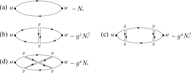
Figure 10: $N_{\text{c}}$ counting for the meson two-point function. (a) Tree-level diagram. (b) First loop correction $g^{2}N_{\text{c}}^{2}\sim N_{\text{c}}$. (c) Next planar loop correction $g^{4}N_{\text{c}}^{3}\sim N_{\text{c}}$. (d) Non-planar loop correction $g^{4}N_{\text{c}}\sim N_{\text{c}}^{-1}$.

The next important observation in the large-$N_{\text{c}}$ limit is that the so-called non-planar diagrams are suppressed by at least $1/N_{\text{c}}^{2}$ as compared to the planar diagrams. To see this, let us consider the two-point function of the meson composite field $M\sim\bar{\psi}\psi$ as drawn in Fig. 10. It is obvious that the tree-level diagram connecting two meson fields consists of simple one-loop with two lines, making a contribution of $\mathcal{O}(N_{\text{c}})$ (see Fig. 10 (a)). The next contribution at the two-loop level is shown in Fig. 10 (b), that has an extra factor by $g^{2}N_{\text{c}}$ than the tree-level contribution. Therefore, in this way, every time the loop order is incremented, a factor $g^{2}N_{\text{c}}$ at least is multiplied. Therefore, to construct the meson two-point function in a non-perturbative and non-diverging way, the strong coupling constant must scale as $g^{2}\sim 1/N_{\text{c}}$ (or so-called ’t Hooft coupling $\lambda\equiv g^{2}N_{\text{c}}$ is kept fixed), and then the contribution from Fig. 10 (b) can be of the same order as (a). The next loop order consists of the planar diagram (c) and the non-planar diagram (d) with an overhead crossing. Now that $g^{2}\sim 1/N_{\text{c}}$, (c) is at the same order as (b), while (d) is suppressed by $1/N_{\text{c}}^{2}$.

The meson two-point function $\langle M(k)M(-k)\rangle$ is of order of $N_{\text{c}}$ as is clear from Fig. 10, that means that the meson decay constant scales like $f_{\pi}\sim\sqrt{N_{\text{c}}}$. From this, it is possible to identify the scaling of the inter-meson coupling. That is, let us consider the $n$-point meson correlation function, that involves $(f_{\pi})^{n}\sim N_{\text{c}}^{n/2}$ and the $n$-point interaction vertex $g_{n}$. The whole planar diagrams should scale as $N_{\text{c}}$, and therefore, $g_{n}\sim N_{\text{c}}^{1-n/2}$. Hence, the inter-meson vertices are all vanishing for $n\geq 3$ in the limit of $N_{\text{c}}\to\infty$. The baryon, on the other hand, is composed from $N_{\text{c}}$ quarks and the baryon mass is thus of $\mathcal{O}(N_{\text{c}})$ (there are $N_{\text{c}}(N_{\text{c}}-1)$ pairs of inter-quark interactions, but the interaction strength scales as $1/N_{\text{c}}$ and then the total scaling is $\mathcal{O}(N_{\text{c}})$) [178]. Then, in QCD with $N_{\text{c}}\to\infty$, baryons are infinitely heavy and the theory is reduced to a system with infinite towers of mesons and glueballs.

3.5.2 Skyrme model

One could construct the baryon as a bound state of $N_{\text{c}}$ quarks. Then, the baryon mass is naturally $\mathcal{O}(N_{\text{c}})\sim\mathcal{O}(1/g^{2})$, while the interaction of low-lying particles is $\mathcal{O}(1/N_{\text{c}})\sim\mathcal{O}(g^{2})$. This inverse-correlation is reminiscent of the properties of the soliton. Indeed, it is possible to construct the baryon as a soliton in terms of the low-lying fields.

Single skyrmion

Here, we shall limit our discussions in the simplest example of the $\mathrm{SU}(2)$ case. The low-energy effective Lagrangian in the non-linear representation again is

$$\mathcal{L}=\frac{f_{\pi}^{2}}{4}\text{tr}\bigl{(}\partial_{\mu}U\partial^{\mu}U^{\dagger}\bigr{)}+\frac{1}{32e^{2}}\text{tr}\bigl{(}\partial_{\mu}UU^{\dagger},\partial_{\nu}UU^{\dagger}\bigr{)}^{2}\;,$$ (89)

if we neglect the infinite tower of mesons and pick up only the pion field. A parameter $e$ which is $\mathcal{O}(\sqrt{N_{\text{c}}})$ is dimensionless and takes a real value. The second term (sometimes called the Skyrme term) is absent in the leading-order ChPT, and the presence of this term is crucially important; the soliton solution would collapse to zero size without this fourth-order derivative term (Derrick’s theorem; this might be relaxed with inclusion of $\omega$ meson, see Ref. [181]).

Introducing a current, $\Sigma_{\mu}=U\partial_{\mu}U^{\dagger}$, the expectation of the Hamiltonian leads to the energy,

$$E=\int d^{3}x\,\text{tr}\biggl{[}\frac{f_{\pi}^{2}}{4}\Sigma_{i}\Sigma_{i}^{\dagger}+\frac{1}{16e^{2}}(\epsilon_{ijk}\Sigma_{i}\Sigma_{j})(\epsilon_{abk}\Sigma_{a}\Sigma_{b})^{\dagger}\biggr{]}\;,$$ (90)

and the baryon current is expressed as $j_{\text{B}}^{\mu}=(1/24\pi^{2})\epsilon^{\mu\nu\alpha\beta}\text{tr}\Sigma_{\nu}\Sigma_{\alpha}\Sigma_{\beta}$, from which one can define the baryon number, $B=\int d^{3}x\,j_{\text{B}}^{0}(x)$. With the following hedgehog Ansatz using a spatial unit vector $\hat{\boldsymbol{r}}=\boldsymbol{r}/r$ for a chiral soliton,

$$U(x)=\exp\bigl{[}iF(r)\boldsymbol{\tau}\cdot\hat{\boldsymbol{r}}\bigr{]}\;,$$ (91)

the energy can be written as a functional of $F$, i.e.

$$E[F]=4\pi\int_{0}^{\infty}dr\,r^{2}\biggl{[}\frac{f_{\pi}^{2}}{2}\Bigl{(}F^{\prime 2}+2\frac{\sin^{2}F}{r^{2}}\Bigr{)}+\frac{1}{2e^{2}}\frac{\sin^{2}F}{r^{2}}\Bigl{(}\frac{\sin^{2}F}{r^{2}}+2{F^{\prime}}^{2}\Bigr{)}\biggr{]}\;,$$ (92)

and the baryon number density is calculated into a form of $j_{\text{B}}^{0}(x)=-F^{\prime}\sin^{2}F/(2\pi^{2}r^{2})$. The baryon number is then properly quantized as

$$B=\frac{1}{2\pi}\bigl{[}2F(0)-\sin 2F(0)\bigr{]}\to 1\;,$$ (93)

if the boundary condition is chosen as $F(0)=\pi$, where we have used $F(\infty)\to 0$.

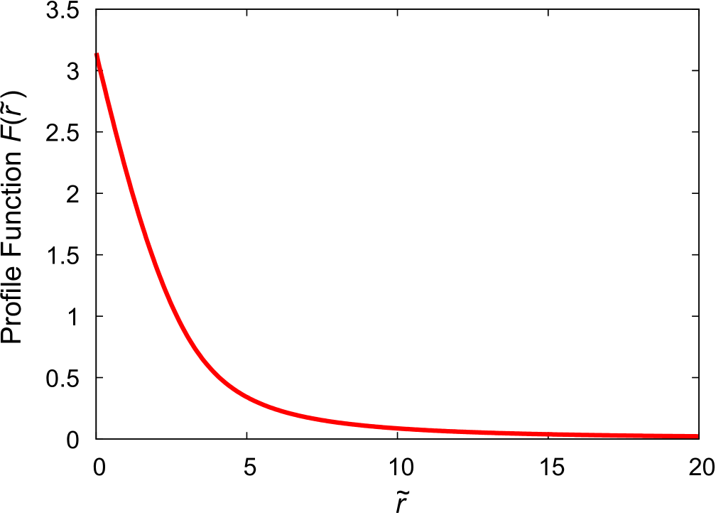
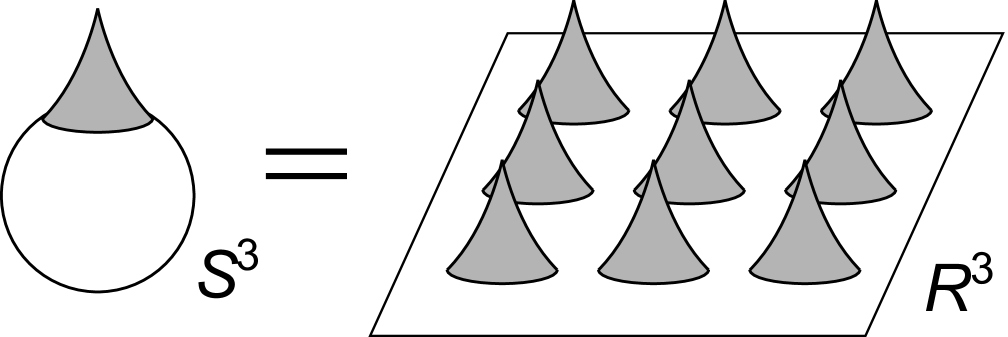
Figure 11: (Left) Profile function $F(\tilde{r})$ as a function of the dimensionless radius variable. The slope at the origin is chosen to satisfy the boundary condition; $F(\tilde{r}\to\infty)\to 0$. (Right) Schematic picture of nuclear matter of skyrmions placed on $S^{3}$.

The concrete form of the pion profile $F(r)$ is determined to minimize the energy (92),

$$\biggl{(}\frac{\tilde{r}^{2}}{4}+2\sin^{2}F\biggr{)}F^{\prime\prime}+\frac{\tilde{r}}{2}F^{\prime}+F^{\prime 2}\sin 2F-\frac{\sin 2F}{4}-\frac{\sin^{2}F\sin 2F}{\tilde{r}^{2}}=0\;.$$ (94)

Here we used a dimensionless variable $\tilde{r}=r/R$ with $R^{-1}=2ef_{\pi}$. The numerical solution that satisfies the proper boundary conditions is plotted in the left panel of Fig. 11. For a more realistic description, one should include strangeness, quantize the solution to give proper quantum numbers such as the angular momentum and the iso-spin, which is beyond our scope of this review.

Nuclear matter as a Skyrme crystal

This pion profile describes a single baryon, and it is necessary to extend the formulation to be capable of including multi-baryons to study the nuclear matter properties. It is not easy to construct skyrmions for $B\gg 1$ directly, but a system at finite density can be emulated with periodically placed skyrmions [182] since baryons are infinitely heavy and static in the large-$N_{\text{c}}$ limit. One can analyze this problem by putting a skyrmion on $S^{3}$, which can be viewed as multi-skyrmions on $R^{3}$ as schematically visualized in the right panel of Fig. 11. This idea has been extended to the skyrmion in the holographic QCD model [183].

Interestingly enough, such a description of skyrmion matter might suggest that nuclear matter in the large-$N_{\text{c}}$ limit could have an inhomogeneous structure in it. Actually, the Skyrme model is based on the non-linear representation of the chiral model as we saw above, and it is impossible to reach chiral restoration, and yet, one can argue chiral restoration as a spatial average of $\langle\text{tr}U\rangle$. This implies that the chiral condensate may have inhomogeneity there, and this is indeed one of the characteristic features in quarkyonic matter as we see in Sec. 4.5.

Half-skyrmions and the Brown-Rho scaling

In Ref. [124] a universal scaling law in dense matter was suggested;

$$\Phi(\rho)=\frac{m_{\text{N}}^{\ast}}{m_{\text{N}}}=\frac{m_{\text{V}}^{\ast}}{m_{\text{V}}}=\frac{f_{\pi}^{\ast}}{f_{\pi}}\;,$$ (95)

where the asterisks are for in-medium quantities and $\Phi$ is a scaling function of density $\rho$. This scaling called the Brown-Rho (BR) scaling is achieved starting with the chiral Lagrangian with the Skyrme term and modifying it such that the correct scaling property expected from QCD is recovered.

The periodic skyrmion configuration is not necessarily optimal in energy and more careful analysis on crystallography should be necessary, which results in BCC and FCC crystal structures involving half-skyrmions [184, 185]. In fact, an intermediate phase where a skyrmion turns into two half-skyrmions was found at some critical density $\rho_{1/2}$ higher than the normal nuclear density $\rho_{0}$ [186, 187], is also observed in the holographic QCD models [188]. For an intriguing implication to the QCD phase diagram, the state with half-skyrmions indicates the presence of the pseudo-gap phase above the chiral phase transition as is suggested in Ref. [189].

It turned out that the meson and baryon masses behave differently in increasing density and the scaling (95) holds fairly well up to the density $\rho_{1/2}$, but above $\rho_{1/2}$, it is significantly deviated [190]. The baryon mass drops at a slower rate than the meson mass with increasing density and stays non-vanishing at chiral symmetry restoration, which matches the chiral invariant mass $m_{0}$ discussed in Sec. 3.3.1. Its consequences on the tensor forces and the EoS at high density are discussed adopting a modified scaling motivated by the above observation in Ref. [190].

3.5.3 Sakai-Sugimoto model

Another non-perturbative approach developed in the large-$N_{\text{c}}$ limit is the holographic technique that is becoming more and more familiar among QCD physicists nowadays. There are countless number of works using the holographic QCD models, and it is not realistic to make an attempt to cover them all. We will pay special attention to the phase diagram disclosed by the Sakai-Sugimoto model, following the computational steps of Ref. [22].

The basic idea of the holographic approach is based on a hypothetical correspondence between a gravity theory in higher dimensions and a field theory of our interest (see Ref. [191] for a review). The original conjecture was made for the $\mathcal{N}=4$ supersymmetric Yang-Mills theory, which at large-$N_{\text{c}}$ and large-’t Hooft coupling may be equivalently described by the classical solution (anti-de Sitter metric) of the super-gravity theory. For the investigation of QCD, however, supersymmetry and conformal symmetry are unwanted and should be gotten rid of. To this end, one can compactify one extra direction and impose the anti-periodic boundary condition to fermionic super-particles, so that unphysical particles become heavy and decouple from the low-lying dynamics (see Fig. 12). This extra direction is denoted by the coordinate $X_{4}$ here.

Figure 12: Geometries in the confined and the deconfined phases. The roles of the (imaginary) time $\tau$ and the extra coordinate $x_{4}$ are swapped from one to the other phase.

In this subsection, to simplify the notation, we use dimensionless variables rescaled by the radius of the AdS space, $R$. That is,

$$\tilde{t}=\frac{t}{R}\;,\qquad\tilde{\boldsymbol{x}}=\frac{\boldsymbol{x}}{R}\;,\qquad\tilde{x}_{4}=\frac{X_{4}}{R}\;,\qquad\tilde{u}=\frac{u}{R}\;,$$ (96)

where the first $(t,\boldsymbol{x})$ refer to the ordinary Minkowski coordinates, $X_{4}$ is the compact direction, and $u$, together with $(t,\boldsymbol{x})$, spans the 5-dimensional AdS space, and the Minkowski space-time resides at the UV edge, $u=\infty$. In what follows, we omit writing the tilde for notational simplicity.

Deconfinement phase transition

In the confined phase at low temperature, the bulk geometry corresponding to the D4-brane background is expressed by the following metric,

$$\text{(Confining geometry)}~{}~{}~{}~{}~{}ds^{2}=u^{3/2}\bigl{[}-dt^{2}+d\boldsymbol{x}^{2}+f(u)dx_{4}^{2}\bigr{]}+\frac{du^{2}}{u^{3/2}f(u)}+u^{1/2}d\Omega_{4}^{2}\;,\\$$ (97)

where $f(u)=1-(u_{\text{KK}}/u)^{3}$ and $u_{\text{KK}}$ is fixed by the size of $x_{4}$ compactification. This above geometry is singular at $u=u_{\text{KK}}$ and to avoid the conical singularity at $u=u_{\text{KK}}$, in the same way as the angle variable in the polar coordinates, the period of $x_{4}$ (denoted by $\delta x_{4}$ here) is uniquely determined that is translated to a mass scale called the Kaluza-Klein mass, i.e.

$$\delta x_{4}=\frac{4\pi}{3u_{\text{KK}}^{1/2}}\qquad\Rightarrow\qquad M_{\rm KK}=\frac{2\pi R^{-1}}{\delta x_{4}}=\frac{3}{2}\sqrt{u_{\text{KK}}}\,R^{-1}\;.$$ (98)

The physical meaning of $M_{\rm KK}$ is a cutoff scale above which super-particles could get excited and the Sakai-Sugimoto model would be no longer a QCD dual. As we will see soon later, the deconfinement transition temperature is smaller than $M_{\rm KK}$ by a factor and the dual description of the phase diagram is indeed closed within the validity region.

In the deconfined phase at finite $T$, on the other hand, the so-called AdS-blackhole solution should be energetically preferred with the metric,

$$\text{(Deconfining geometry)}~{}~{}~{}~{}~{}ds^{2}=u^{3/2}\bigl{[}-f(u)dt^{2}+d\boldsymbol{x}^{2}+dx_{4}^{2}\bigr{]}+\frac{du^{2}}{u^{3/2}f(u)}+u^{1/2}d\Omega_{4}^{2}\;,$$ (99)

where the singularity in $x_{4}$ is replaced in the temporal direction. In Eq. (99) the definition of the function $f(u)$ is changed to $f(u)=1-(u_{T}/u)^{3}$ with $u_{T}$ fixed by the period as in Eq. (98). In Euclidean space-time with $\tau=it$ the period of $\tau$, that is nothing but the temperature inverse $1/T$, leads to

$$\frac{1}{T}=\frac{4\pi}{3u_{T}^{1/2}}\;.$$ (100)

Therefore, the location of the horizon at $u=u_{T}$ corresponds to the physical temperature $T$.

One can then evaluate the free energy to identify which of the confining and the deconfining metric is more favored and what the critical temperature $T_{\text{d}}$ is. We can easily make a theoretical guess for $T_{\text{d}}$ from the corresponding geometries illustrated in Fig. 12. Obviously the energies (or actions) should be identical when two periods coincide. That is, the first-order phase transition (Hawking-Page-type transition) should take place [192] when

$$\delta x_{4}=\frac{1}{T}\qquad\Rightarrow\qquad T_{\text{d}}=\frac{3}{4\pi}\sqrt{u_{\text{KK}}}\,R^{-1}=\frac{M_{\rm KK}}{2\pi}\;.$$ (101)

On the phenomenological level $M_{\rm KK}$ is fixed to be $949\;\text{MeV}$ to reproduce the vector meson spectrum, so that $T_{\text{d}}\simeq 151\;\text{MeV}$ is obtained, which is of the same order as the empirical value presented in Sec. 2.3. In the leading order of the large-$N_{\text{c}}$ approximation this critical temperature for deconfinement is insensitive to the presence of matter and, as discussed in Sec. 3.5.1, this is simply because quarks are suppressed by $1/N_{\text{c}}$ as compared to gluons.

We here make a remark on the weak-coupling extrapolation with non-trivial $\beta$ function. This may lead to a possibility of disconnection between deconfinement in the strong-coupling and the weak-coupling regimes [193].

Flavor branes

Let us now turn to chiral symmetry realized in the Sakai-Sugimoto model [23] and the chiral phase transition. The same chiral symmetry as QCD, i.e. $\mathrm{U}_{\text{L}}(N_{\text{f}})\times\mathrm{U}_{\text{R}}(N_{\text{f}})$, can be emulated by putting $N_{\text{f}}$ D8-branes localized at $x_{4}=0$ and $N_{\text{f}}$ $\overline{\rm D8}$-branes at $x_{4}=L$. This $L$ is a parameter inherent in the Sakai-Sugimoto model and its physical interpretation in QCD is still unclear. For the meaning of the lower edge $u_{c}$, see Fig. 13. We will explain how to fix $u_{c}$ when we incorporate the density source next. In the large-$N_{\text{c}}$ limit the D4-brane is dominant and one can assume that the classical solutions are intact regardless of flavor branes (that is, the probe approximation), which corresponds to quark suppression by $1/N_{\text{c}}$.

Figure 13: Flavor branes (D8 and $\overline{\rm D8}$ separated by the length parameter $L$) in the confined and the deconfined phases. In the confined phase chiral symmetry is inevitably broken, while in the deconfined phase both chiral broken and symmetric states are realized.

The induced metric on the D8-branes is (apart from the spherical angular part, $\Omega_{4}$), thus,

$$\text{(Confining geometry)}~{}~{}~{}~{}~{}~{}ds^{2}=u^{3/2}\bigl{(}-dt^{2}+d\boldsymbol{x}^{2}\bigr{)}+\biggl{[}u^{3/2}f(u){x_{4}^{\prime}(u)}^{2}+\frac{1}{u^{3/2}f(u)}\biggr{]}du^{2}\;,$$ (102)

$$\text{(Deconfining geometry)}~{}~{}~{}ds^{2}=u^{3/2}\bigl{(}-f(u)dt^{2}+d\boldsymbol{x}^{2}\bigr{)}+\biggl{[}u^{3/2}{x_{4}^{\prime}(u)}^{2}+\frac{1}{u^{3/2}f(u)}\biggr{]}du^{2}\;.$$ (103)

Here $x_{4}(u)$ is solved with the equation of motion later. To introduce a finite density, we need a gauge field $A_{0}(u)$ that becomes the quark chemical potential at $u=\infty$. We can then express the Dirac-Born-Infeld (DBI) action involving the gauge fields on the $N_{\text{f}}$ D8-brane, after integrating over the four-dimensional angular part $\Omega_{4}$, as

$$S_{\text{D8}}^{\text{DBI}}=-\frac{\mathcal{N}}{V_{4}}\int dt\,d^{3}x\,du\,u^{1/4}\sqrt{-\det(g_{\alpha\beta}+F_{\alpha\beta})}\;.$$ (104)

Here the dilaton potential is already included in the action and the field strength tensor in the above is rescaled to eliminate the string scale $l_{s}$ (see Refs. [23, 22] for details). The normalization constant including the $\Omega_{4}$ integration is given as $\mathcal{N}=V_{4}\cdot(N_{\text{c}}N_{\text{f}}/3)R^{6}/((2\pi)^{5}l_{s}^{6})$ with $V_{4}=\int dt\,d^{3}x$.

In Euclidean space-time at finite $T$, integrating further over the Euclidean coordinates, we can express the action in a form of the one-dimensional integration with respect to $u$. Hereafter we drop the irrelevant normalization $\mathcal{N}$ from the action and then the action simplifies, respectively, in the confined and the deconfined phases as

$$\text{(Confining geometry)}~{}~{}~{}~{}~{}~{}~{}~{}~{}~{}~{}~{}S_{\text{D8}}^{\text{DBI}}=\int du\,u^{4}\sqrt{f(u)x_{4}^{\prime}(u)^{2}+\frac{1}{u^{3}}\bigl{(}{f(u)}^{-1}-a_{0}^{\prime 2}\bigr{)}}\;,$$ (105)

$$\text{(Deconfining geometry)}~{}~{}~{}~{}~{}~{}~{}~{}~{}S_{\text{D8}}^{\text{DBI}}=\int du\,u^{4}\sqrt{f(u)x_{4}^{\prime}(u)^{2}+\frac{1}{u^{3}}(1-a_{0}^{\prime 2})}\;,$$ (106)

where $a_{0}(u)$ denotes the rescaled $A_{0}(u)$ that eventually translates to the (dimensionless) chemical potential. It is convenient to use a density variable $\rho(u)=-\delta S_{\text{D8}}^{\text{DBI}}/\delta a_{0}^{\prime}(u)$, because $\rho(u)$ turns out to be $u$-independent thanks to the equation of motion. Then, we can easily solve $a_{0}^{\prime}(u)$ from the definition of $\rho$ to find,

$$\text{(Confining geometry)}~{}~{}~{}~{}~{}~{}~{}~{}~{}~{}~{}a_{0}^{\prime}(u)=\rho\,\sqrt{\frac{u^{3}f(u)^{2}{x_{4}^{\prime}(u)}^{2}+1}{f(u)(u^{5}+\rho^{2})}}\;,$$ (107)

$$\text{(Deconfining geometry)}~{}~{}~{}~{}~{}~{}~{}~{}a_{0}^{\prime}(u)=\rho\,\sqrt{\frac{u^{3}f(u)\,{x_{4}^{\prime}(u)}^{2}+1}{u^{5}+\rho^{2}}}\;,$$ (108)

from which the quark chemical potential $\mu_{\text{q}}=a_{0}(\infty)$ is obtained in respective phases.

Introduction of the density source

Here we shall explain how to fix the lower boundary $u_{c}$ displayed on Fig. 13. If the system is in the deconfined and chiral symmetric phase at high $T$, D8 and $\overline{\rm D8}$ are parallel and such a configuration can have a finite density without source, and thus $u_{c}$ is not necessary and the $u$-integration starts simply from $u_{T}$.

When chiral symmetry is spontaneously broken, on the other hand, there should be a source for the density coming from the Chern-Simons action. To accommodate a finite density of baryonic matter, instantons or the D4-branes wrapped on the $S^{4}$ inside of the D8-branes should be placed, as argued in Ref. [194], in a similar way as the skyrmion in Sec. 3.5.2. In the confined phase baryons are the unique source for the density, while quark matter is also possible in the deconfined phase. Such a density source originating from quarks can be formulated as strings stretched from the D8-branes to the horizon. It is known, however, that such a density source leads to a larger action (i.e. larger free energy) than the instanton source [22], which means that baryonic matter is always favored than quark matter in this model. This observation might be given a deeper insight from the concept of quarkyonic matter that is the main subject of Sec. 4.5.

The point where the density source is placed along the $u$-direction defines $u_{c}$ and its value is dynamically determined by the zero-force condition. In the presence of the source the flavor-branes are pulled and $x_{4}(u)$ has a cusp at $u=u_{c}$, as illustrated in Fig. 13, and the range of the $u$-integration should be from $u_{c}$ to $+\infty$. The zero-force condition describes a situation that the tension of the D8-branes $f_{\text{D8}}$ should be balanced by the force from the source D4-brane $f_{\text{D4}}$. These forces can be given by the derivative of corresponding actions with respect to $u_{c}$.

Deconfined and chiral symmetric phase

On the phase diagram we will find a first-order phase transition associated with the restoration of chiral symmetry, and then the density $\rho$ jumps discontinuously. So, to distinguish the densities in respective phases, let us denote the density in the chiral symmetric phase as $\rho_{\text{sym}}$, while we use $\rho_{\text{broken}}$ in the chiral broken phase.

When chiral symmetry is restored at sufficiently high temperature, D8 and $\overline{\rm D8}$ are straight and parallel (the far left of Fig. 13). In this case the solution of the equation of motion is as simple as $x_{4}^{\prime}(u)=0$. Then, we do not have to introduce a source term but the horizon at $u=u_{T}$ can take care of the role as a density source. The physical chemical potential is obtained from $\mu_{\text{q}}=a_{0}(\infty)$, that is,

$$\mu_{\text{q}}=\rho_{\text{sym}}\int_{u_{T}}^{\infty}du\,\frac{1}{\sqrt{u^{5}+\rho_{\text{sym}}^{2}}}\;,$$ (109)

from Eq. (108). The thermodynamic potential is then calculated from the action (106) as

$$\Omega_{\text{sym}}=\int_{u_{T}}^{\infty}du\,\frac{u^{5}}{\sqrt{u^{5}+\rho_{\text{sym}}^{2}}}\;.$$ (110)

Deconfined and chiral broken phase

The treatment of the chiral broken phase is much more complicated than the chiral symmetric phase because the configuration of D8-branes should be numerically solved from the Euler-Lagrange equation from the action (106) as

$$x_{4}^{\prime}(u)=\frac{\sqrt{f(u_{0})(u_{0}^{8}+\rho_{\text{broken}}^{2}u_{0}^{3})}}{u^{3/2}\sqrt{f(u)\bigl{[}f(u)(u^{8}+\rho_{\text{broken}}^{2}u^{3})-f(u_{0})(u_{0}^{8}+\rho_{\text{broken}}^{2}u_{0}^{3})\bigr{]}}}\;,$$ (111)

where $u_{0}$ is defined by a point where $x_{4}^{\prime}(u_{0})$ diverges. Then, in this phase, the chemical potential is expressed from Eq. (108) as

$$\mu_{\text{q}}=\rho_{\text{broken}}\int_{u_{c}}^{\infty}du\,\sqrt{\frac{f(u)u^{3}}{f(u)(u^{8}+\rho_{\text{broken}}^{2}u^{3})-f(u_{0})(u_{0}^{8}+\rho_{\text{broken}}^{2}u_{0}^{3})}}+\frac{u_{c}}{3}\sqrt{f(u_{c})}\;.$$ (112)

We note that the second term in the right-hand side is added by the D4-brane contribution in the presence of density, and this determines the threshold $\mu_{\text{q}}$ for finite density. Such an onset of the density corresponds to $m_{\text{N}}-B/A$ in nuclear matter; we have already seen $\rho=0$ as long as $\mu_{\text{B}}<m_{\text{N}}-B/A$ (see the right panel of Fig. 7). In other words, if $\mu_{\text{q}}$ is smaller than this threshold value, the only possible solution is $\rho_{\text{broken}}=0$ and the ground state is matter-free empty. We should concretely figure out the lower edge of the integration, $u_{c}$, to proceed in the calculation. The zero-force condition, $f_{\text{D8}}=f_{\text{D4}}$, yields [22],

$$\sqrt{\frac{f(u_{c})(u_{c}^{8}+\rho^{2}u_{c}^{3})-f(u_{0})(u_{0}^{8}+\rho^{2}u_{0}^{3})}{f(u_{c})u_{c}^{3}}}=\frac{\partial}{\partial u_{c}}\,\frac{\rho}{3}\,u_{c}\sqrt{f(u_{c})}\;.$$ (113)

The thermodynamic potential in the chiral broken phase is, thus, obtained from the action, which amounts to

$$\Omega_{\text{broken}}=\int_{u_{c}}^{\infty}du\,\frac{\sqrt{f(u)\,u^{3}}\,u^{5}}{\sqrt{f(u)(u^{8}+\rho_{\text{broken}}^{2}u^{3})-f(u_{0})(u_{0}^{8}+\rho_{\text{broken}}^{2}u_{0}^{3})}}\;.$$ (114)

The above-mentioned setup suffices for the determination of the chiral phase transition point by the comparison between Eqs. (110) and (114). The concrete procedure for this is as follows: First, for a given density $\rho_{\text{broken}}$, the zero-force condition (113) gives $u_{c}(u_{0},T)$, and this renders the condition $L=2\int_{u_{c}}^{\infty}x_{4}^{\prime}(u)du$ expressed as a function of $u_{0}$. This enables us to solve $u_{0}(\rho_{\text{broken}},L,T)$, so that Eq. (112) directly relates $\mu_{\text{q}}$ and $\rho_{\text{broken}}$. Then we get $\Omega_{\text{broken}}(L,T,\mu_{\text{q}})$ finally. In the same (and much simpler) way, we can calculate $\Omega_{\text{sym}}(L,T,\mu_{\text{q}})$, and we can locate the first-order Hawking-Page transition of chiral restoration by looking for $T$ and $\mu_{\text{q}}$ that makes $\Omega_{\text{broken}}=\Omega_{\text{sym}}$. In this way, particularly at vanishing $\mu_{\text{q}}$, the critical temperature turns out to be $T_{\chi}=0.154/L$, which was first found in Ref. [195].

Density onset and the phase diagram

The phase diagram is not yet complete. We should consider another line corresponding to the liquid-gas phase transition as presented explicitly in the conventional description in the right panel of Fig. 7.

In the confined phase chiral symmetry is always broken. The equation of motion for $x_{4}^{\prime}(u)$ is slightly different from Eq. (111) and is given by

$$x_{4}^{\prime}(u)=\sqrt{\frac{f(u_{0})(u_{0}^{8}+\rho_{\text{broken}}^{2}u_{0}^{3})}{u^{3}f(u)^{2}[f(u)(u^{8}+\rho_{\text{broken}}^{2}u^{3})-f(u_{0})(u_{0}^{8}+\rho_{\text{broken}}^{2}u_{0}^{3})]}}\;,$$ (115)

from which the zero-force condition results in a similar form to Eq. (113) in which the right-hand side is replaced with $\partial(\rho u_{c}/3)\partial u_{c}$. The onset at which a finite density is turned on can be found analytically with $\rho_{\text{broken}}=0$ plugged into the above equations. Then, we simply have $u_{c}=u_{0}$, and the corresponding chemical potential is $\mu_{\text{q}}=u_{0}/3$. At the onset we can approximate (115) with $f(u)\simeq 1$ to derive $u_{0}$ analytically, and the critical $\mu_{\text{q}}$ is then obtained as $(4\pi/3)(\Gamma[9/16]/\Gamma[1/16])^{2}\simeq 0.175$ in the unit of $L$. In the deconfined phase, on the other hand, the density onset lies at $\mu_{\text{q}}=(u_{0}/3)\sqrt{f(u_{0})}$, which is $T$-dependent. Then, the phase boundary is not a straight vertical line but it has a minor dependence on $T$.

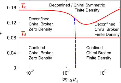
Figure 14: Phase diagram at finite temperature and density in the Sakai-Sugimoto model. The deconfinement temperature is chosen at $T_{\text{d}}=0.08$ and the scale is set by $L=1$ according to the choice of Ref. [22]. The vertical dashed line represents the onset of baryon density.

Some numerical calculations are needed to clarify the whole phase structure, and the resulting phase diagram is depicted in Fig. 14, which first appeared in Ref. [22]. This is a quite suggestive phase diagram, but we shall defer a more detailed comparison between Fig. 14 and the expected phase structure of large-$N_{\text{c}}$ QCD till Sec. 4.5.

We here raise some caveats; the above treatment is based on the probe approximation that corresponds to the quench limit of QCD, and the $1/N_{\text{c}}$ corrections should be considered to take account of back-reactions from matter. For more details including other holographic models than the Sakai-Sugimoto model, see a recent review [196]. This is not yet the end of the story about the phase diagram in the Sakai-Sugimoto model. Recently there has been an important recognition; an instability of gauge fluctuations at non-zero momenta was discovered at finite density [197, 198], and so, the phase diagram in Fig. 14 must be supplemented with additional phase boundaries associated with spatial modulations (see Fig. 1 of Ref. [197] for instance).

It is quite interesting to notice that this sort of spatially inhomogeneous structure was once discussed actively in the context of nuclear physics, and nowadays, is becoming one of the central issues in quark matter research. Here, for a while, it should be worth revisiting the possibility of inhomogeneous condensation in nuclear matter.

3.6 Inhomogeneity: pion condensation

In a medium at finite density there are collective excitations made from particle and hole ($p$-$h$) in the same channel as pions. The interaction between $N$ and $\pi$ is, however, repulsive in the $s$-wave channel and the pion self-energy is positive then. It was recognized later in Refs. [199, 200] that the $p$-wave interaction is attractive, which causes a resonant state $\Delta$ in the channel of $L=1$, $J=3/2$, $T=3/2$, and it would render the pion energy decrease in matter. This attractive interaction is attributed to underlying chiral symmetry.

The in-medium pion propagator can be written with the self-energy as

$$D_{\pi}^{-1}(\omega,\boldsymbol{p})=\omega^{2}-\boldsymbol{p}^{2}-m_{\pi}^{2}-\Pi(\omega,\boldsymbol{p})\;,$$ (116)

where the self-energy $\Pi(\omega,\boldsymbol{p})$ should involve the $p$-$h$ and $\Delta$-$h$ contributions; $\Pi=-p^{2}[U_{N}(\omega,\boldsymbol{p})+U_{\Delta}(\omega,\boldsymbol{p})]$. In the symmetric nuclear matter with $Z=N$ that is of our main interest, the collective mode is pushed down at finite $\boldsymbol{p}$ and there appears a condensate of $\pi^{0}$, while in neutron matter which is relevant to the astrophysical application the collective $\pi^{+}$ (Migdal’s $\pi_{s}^{+}$) and $\pi^{-}$ are spontaneously generated [200].

When the $\pi^{0}$ condensation occurs in symmetric nuclear matter at the momentum $\boldsymbol{p}_{c}$, the expectation value should behave as

$$\langle\pi^{0}(\boldsymbol{x},\boldsymbol{p}_{c})\rangle\;\sim\;\cos(\boldsymbol{p}_{c}\cdot\boldsymbol{x})\;.$$ (117)

The physical implication of such condensate to nuclear matter has been discussed (see Ref. [201] and other contributions in this volume).

One can find the critical density for the $\pi^{0}$ condensation, for instance, adopting the linear sigma model including $p$, $n$, and $\Delta$’s. Once the density exceeds the threshold, however, the system is unstable because only the attractive force is taken into account and the short-range (shorter than the pion Compton length) repulsive interaction between baryons should be considered. In the Fermi liquid theory such short-range $NN$ interactions (proportional to $\delta(\boldsymbol{x}_{1}\!-\!\boldsymbol{x}_{2})$) are incorporated through the Landau parameters in the following form;

$$F_{NN}=f_{NN}+f^{\prime}_{NN}\boldsymbol{\tau}_{1}\cdot\boldsymbol{\tau}_{2}+g_{NN}\boldsymbol{\sigma}_{1}\cdot\boldsymbol{\sigma}_{2}+\biggl{(}\frac{f_{\pi NN}^{2}}{m_{\pi}^{2}}\biggr{)}g^{\prime}_{NN}(\boldsymbol{\sigma}_{1}\cdot\boldsymbol{\sigma}_{2})(\boldsymbol{\tau}_{1}\cdot\boldsymbol{\tau}_{2})\;.$$ (118)

Here $\boldsymbol{\tau}_{1}$ and $\boldsymbol{\sigma}_{1}$ (and $\boldsymbol{\tau}_{2}$ and $\boldsymbol{\sigma}_{2}$) refer to the isospin and the spin of nucleon 1 (and nucleon 2, respectively) in the $NN$ system. In fact this last term is required to cancel Dirac’s delta function appearing in the one-pion exchange potential (OPEP) (if $g_{NN}^{\prime}=1/3$ is chosen, the attractive delta function in the OPEP is exactly canceled). Such a cancellation is a universal phenomenon; the Lorentz-Lorenz effect in dielectric media is the most famous example. In the same manner, including the mixing with isobars, one should further consider the Landau-Migdal parameters as

$$F_{N\Delta}=\biggl{(}\frac{f_{\pi NN}f_{\pi N\Delta}}{m_{\pi}^{2}}\biggr{)}g^{\prime}_{N\Delta}(\boldsymbol{\sigma}_{1}\cdot\boldsymbol{\sigma}_{2}^{\Delta})(\boldsymbol{\tau}_{1}\cdot\boldsymbol{\tau}_{2}^{\Delta})\;,\quad F_{\Delta\Delta}=\biggl{(}\frac{f_{\pi N\Delta}^{2}}{m_{\pi}^{2}}\biggr{)}g^{\prime}_{\Delta\Delta}(\boldsymbol{\sigma}_{1}^{\Delta}\cdot\boldsymbol{\sigma}_{2}^{\Delta})(\boldsymbol{\tau}_{1}^{\Delta}\cdot\boldsymbol{\tau}_{2}^{\Delta})\;,$$ (119)

all of which contribute to $U_{N}(\omega,\boldsymbol{p})$ and $U_{\Delta}(\omega,\boldsymbol{p})$. Because $g_{NN}^{\prime}$, $g_{N\Delta}^{\prime}$, and $g_{\Delta\Delta}^{\prime}$ represent the effect of repulsive interactions, they would disfavor the pion condensation. Therefore, the precise determination of these parameters is fatally important to judge whether the pion condensation can occur or not in reality.

Today it is widely believed that the possibility of the pion condensation in nuclear matter was somehow ruled out. This was concluded from the experimental data of the giant Gamow-Teller (GT) states which are collective modes with respect to the spin-isospin fluctuations, so that their strength can constrain $g_{NN}^{\prime}$, $g_{N\Delta}^{\prime}$, and $g_{\Delta\Delta}^{\prime}$ (see Ref. [202] for a review). Since the decomposition is difficult, it used to be often the case to assume the universality, $g_{NN}^{\prime}=g_{N\Delta}^{\prime}=g_{\Delta\Delta}^{\prime}=g^{\prime}$, and then the experimental data suggests $g^{\prime}=0.6\sim 0.9$, which is much larger than $1/3$ and the pion condensation cannot occur in a reasonable range of baryon density. Later on, in theory and experiment, different values of $g^{\prime}$ have been investigated [203], and as comprehensively reviewed in Ref. [204]. Although the pion condensation is unlikely at normal nuclear density $\rho_{0}$, the fact is that there is still a good deal of chance for the $p$-wave pion condensation to develop in nuclear matter at $\rho\gtrsim 2\rho_{0}$. According to Ref. [204], the critical density $\rho_{c}$ is calculated with $g_{NN}^{\prime}=0.59$ and $g_{N\Delta}^{\prime}=0.18+0.05g_{\Delta\Delta}^{\prime}$ fixed from the experimental data, which results in $\rho_{c}=(1.2\sim 2)\rho_{0}$ for the undetermined parameter $g_{\Delta\Delta}^{\prime}=0\sim 1$. This makes a sharp contrast to $\rho_{c}$ under the universality Ansatz, which rapidly grows up to unrealistic density. Definitely, the possibility of the pion condensation should deserves more investigations. As we will see later in Sec. 4.4, an interesting form of the inhomogeneous condensate analogous to the condensate (117) is a likely candidate for the ground state of quark matter.

4 Quark/Quarkyonic Matter

In this section we address the properties and the phase transition in deconfined quark matter assuming that the ground state of high density matter is composed from quasi-quarks. First we will make a quick review over a phenomenological description of deconfinement, and then continue our discussions utilizing chiral effective models. Finally we will closely discuss the possibility of inhomogeneous chiral condensate and the general mechanism that would derive inhomogeneity at high density.

4.1 Statistical bootstrap and the Hagedorn limiting temperature

In quantum field theories we are still far from satisfactory understanding of confinement and deconfinement. In phenomenology, however, it is quite useful (and probably a right picture) to think of the Hagedorn spectrum. Let us denote the density of states $\rho(m^{2})$ so that $\rho(m^{2})dm$ counts the number of hadronic states in the mass range $m\sim m+dm$. The idea of the statistical bootstrap model is that hadronic states are composed from a convolution of smaller hadrons. This picture is embodied as the following statistical bootstrap equation for the hadron mass spectrum [205],

$$H\rho(p^{2})=H\theta(p_{0})\delta(p^{2}-m_{\rm in}^{2})+\sum_{N=2}^{\infty}\frac{1}{N!}\int\delta^{(4)}(p-\sum_{i}^{N}p_{i})\prod_{i=2}^{N}H\rho(p_{i}^{2})d^{4}p_{i}\;,$$ (120)

where $H$ represents a proper hadronic volume and $m_{\rm in}$ is an input parameter corresponding to the “elementary” mass in the bootstrap picture. Interestingly, it is possible to fix the asymptotic form of $\rho(m^{2})$ semi-analytically from the above equation. Introducing the Laplace transforms of Eq. (120) as $G(\beta)=\int e^{-\beta p}H\rho(p^{2})d^{4}p$ and $\varphi(\beta)=\int e^{-\beta p}H\theta(p_{0})\delta(p^{2}\!-\!m_{\rm in}^{2})d^{4}p$, where $\beta$ corresponds to the temperature in the Boltzmann factor, the bootstrap equation (120) is rewritten into a simple form;

$$G(\beta)=\varphi(\beta)+e^{G(\beta)}-G(\beta)-1\;.$$ (121)

Although it is not easy to solve $G$ as a function of $\varphi$, Eq. (121) already solves $\varphi$ in terms of $G$; $\varphi=2G+1-e^{G}$, which has a maximum and we shall denote this extremal point by $\varphi_{0}$, and this $\varphi_{0}$ can be converted to corresponding $\beta_{0}$. Then, $G(\beta)$ can be expanded around $\beta_{0}$, i.e. $G(\beta)\simeq G(\beta_{0})+\text{(const.)}(\beta-\beta_{0})^{1/2}$. Such a type of square-root singularity can be reproduced by the density of states,

$$\rho(m^{2})=C\,m^{-3}e^{m/T_{\text{H}}}\;,$$ (122)

where $T_{\text{H}}$ is a temperature parameter (related to $\beta_{0}$) and called the Hagedorn temperature. This exponential form of the density of hadronic states is an important observation in understanding the physics of deconfinement at the phenomenological level.

The physical interpretation of the Hagedorn temperature is quite instructive. The partition function, $\int\rho(m)e^{-m/T}dm$, would diverge when $T>T_{\text{H}}$ and thus the physical temperature cannot exceed $T_{\text{H}}$ as long as the hadronic description is valid. In this sense $T_{\text{H}}$ used to be considered as the limiting temperature. In Ref. [24] it was argued that $T_{\text{H}}$ should be the critical temperature where the hadronic description breaks down and the system goes through a phase transition into deconfined quarks. Actually the very first prototype of the QCD phase diagram was conjectured in Ref. [24] based on this interpretation of $T_{\text{H}}$. In a modern language stemming from the Hagedorn picture, the deconfinement phenomenon is correctly captured by the thermal statistical model or the hadron resonance gas model (see also Sec. 4.5.2).

4.2 Chiral effective models

Once quark deconfinement occurs, the most suited description of the state of matter should be of interacting quarks rather than mesons and baryons. It is still challenging to tackle the QCD phase transitions from the first principle unless the the quark density is so small that the lattice-QCD is at work. Then, for the pragmatic studies on the QCD phase diagram, one can adopt an effective model that shares common physical features with QCD, and chiral symmetry is the guiding principle for the model building.

4.2.1 Nambu–Jona-Lasinio model

At sufficiently high density it is conceivable that the physical degrees of freedom should be quarks rather than baryons, and then it makes sense to consider a picture of quasi-quarks as a result of integrating out heavy gluonic degrees of freedom. A recent attempt along this line is found in Ref. [206].

In this context the Nambu–Jona-Lasinio (NJL) model is one of the most preferable choices of the low-lying QCD models (for reviews, see Refs. [207, 208]). In principle, the integration over gluons would lead to an infinite number of interactions in terms of quark fields, which can be expanded according to the power of $\bar{\psi}$ and $\psi$ as

$$\mathcal{L}=\bar{\psi}(i\gamma_{\mu}\partial^{\mu}-m_{0})\psi+\mathcal{L}_{\text{int}}^{(4)}(\bar{\psi},\psi)+\mathcal{L}_{\text{int}}^{(6)}(\bar{\psi},\psi)+\cdots\;,$$ (123)

where $\mathcal{L}_{\rm int}^{(4)}$ represents the interaction terms at the quartic order in terms of quark fields, $\mathcal{L}_{\rm int}^{(6)}$ at the sixth order, etc. In the vicinity of the chiral phase transition only $\mathcal{L}_{\rm int}^{(4)}$ is predominantly important in the mean-field analysis (if it is of second order and the mean-field mass is vanishingly small), and we will keep this leading-order interaction only in this article (see Ref. [209] for an extension with higher-order interactions). If the above $\mathcal{L}$ is designed to mimic the QCD dynamics, $\mathcal{L}$ should be invariant under the symmetries of the QCD Lagrangian as exposited in Sec. 2. Motivated by the presence of the chiral condensate in the scalar channel, we should retain the interaction involving the scalar channel in $\mathcal{L}_{\rm int}^{(4)}$, and naturally, $\mathcal{L}_{\rm int}^{(4)}$ should contain the interaction in the pseudo-scalar channel as the chiral partner, which leads to

$$\mathcal{L}_{\text{int}}^{(4)}=\frac{g_{s}}{2}\bigl{[}(\bar{\psi}\lambda_{a}\psi)^{2}+(\bar{\psi}i\gamma_{5}\lambda_{a}\psi)^{2}\bigr{]}-g_{v}(\bar{\psi}\gamma_{\mu}\psi)^{2}\;.$$ (124)

Here the scalar part $(\bar{\psi}\lambda_{a}\psi)^{2}$ and the pseudo-scalar part $(\bar{\psi}i\gamma_{5}\lambda_{a}\psi)^{2}$ are both necessary to be consistent with chiral symmetry, whilst the second term $(\bar{\psi}\gamma_{\mu}\psi)^{2}$ is chiral symmetric as it is. In the NJL model study in the vacuum, this vector interaction has only a minor effect except for the vector mesons, but at finite density we must not neglect it. As a matter of fact, this vector interaction plays an equivalent role as the term $(m_{\omega}^{2}/2)\omega_{\mu}\omega^{\mu}$ in the Walecka model (45).

In QCD at the quantum level $\mathrm{U(1)_{A}}$ symmetry is explicitly broken due to the axial anomaly, which should give rise to the instanton-induced interaction, as already derived in Eq. (28). Because the determinant in flavor space should be taken, the instanton-induced interaction is the four-quark interaction for $N_{\text{f}}=2$ and the six-quark interaction for $N_{\text{f}}=3$, and written then as

$$\mathcal{L}_{\text{int}}^{(6)}=g_{d}\bigl{[}\det\bar{\psi}(1-\gamma_{5})\psi+\det\bar{\psi}(1+\gamma_{5})\psi\bigr{]}\;.$$ (125)

The model parameters, $g_{s}$, $g_{v}$, $g_{d}$, and the UV cutoff $\Lambda$ are fixed so as to reproduce the hadron properties in the vacuum. In general these parameter should vary with changing $T$ and $\mu_{\text{q}}$, but there is no reliable strategy for the determination of such medium dependence. Thus, in the model studies, one usually assumes that one can keep using the same parameters as fixed at $T=\mu_{\text{q}}=0$, which brings in the most unmanageable uncertainty in theory.

Mean-field approximation in the vacuum

The thermodynamic potential is composed from three individual contributions in the simplest mean-field approximation of the NJL model. That is,

$$\Omega=\Omega_{\text{cond}}+\Omega_{\text{zero}}+\Omega_{\text{quark}}\;,$$ (126)

where the three contributions come from the condensation energy, the zero-point oscillation energy, and the quasi-quark partition function. Let us take a look at respective contributions in order below.

The condensation energy comes from the vacuum expectation value of the quark composite operator. The four-point interaction vertex of $u$-quarks, for example, can be approximated as

$$(\bar{u}u)^{2}=(\bar{u}u-\langle\bar{u}u\rangle+\langle\bar{u}u\rangle)^{2}\simeq\langle\bar{u}u\rangle+2\langle\bar{u}u\rangle(\bar{u}u-\langle\bar{u}u\rangle)=-\langle\bar{u}u\rangle^{2}+2\langle\bar{u}u\rangle\bar{u}u\;.$$ (127)

Here we have ignored second-order infinitesimals, $(\bar{u}u-\langle\bar{u}u\rangle)^{2}$. Then, in the final expression above, $-\langle\bar{u}u\rangle^{2}$ is the condensation energy and the second term amounts to the dynamical mass term for $u$-quarks, which should be taken into account in the quasi-quark partition function as the constituent quark mass. It should be mentioned that there is no mixing between different flavors like $\bar{u}u\bar{d}d$ from $\mathcal{L}_{\rm int}^{(4)}$ but the flavor mixing interaction appears solely from the anomaly terms; for $N_{\text{c}}=3$ for instance, the determinant interaction in Eq. (125) causes the flavor mixing. Including the terms $\mathcal{L}_{\rm int}^{(6)}$ for $N_{\text{f}}=3$, the condensation energy amounts in total to

$$\Omega_{\text{cond}}=g_{s}(\langle\bar{u}u\rangle^{2}+\langle\bar{d}d\rangle^{2}+\langle\bar{s}s\rangle^{2})+4g_{d}\langle\bar{u}u\rangle\langle\bar{d}d\rangle\langle\bar{s}s\rangle\;.$$ (128)

In the NJL model the zero-point oscillation energy is essential to bring about the spontaneous breaking of chiral symmetry. Because the NJL model is non-renormalizable, the momentum integration needs a UV cutoff $\Lambda$. In a naïve momentum cutoff scheme the diverging zero-point oscillation energy is expressed as

$$\Omega_{\text{zero}}=-2\cdot 2N_{\text{c}}\sum_{i}\int^{\Lambda}\frac{d^{3}p}{(2\pi)^{3}}\,\frac{\varepsilon_{i}(p)}{2}\;,$$ (129)

where the overall factor $2\cdot 2$ is from the spin and the particle and anti-particle degeneracy, and $N_{\text{c}}=3$ is the number of colors. For a more sophisticated treatment with non-local interactions that tame the UV divergence, see Refs. [210, 211, 212, 213]. We also note that the non-local formulation is already close to the Dyson-Schwinger approach [214]. The quasi-particle energy $\varepsilon_{i}(p)$ depends on the flavor which is indicated by the index $i$. In the mean-field approximation, together with the second term of Eq. (127), the quasi-quarks should have the constituent quark masses;

$$M_{i}=m_{i}-2g_{s}\langle\bar{\psi}_{i}\psi_{i}\rangle-g_{d}\,\epsilon_{ijk}\langle\bar{\psi}_{j}\psi_{j}\rangle\langle\bar{\psi}_{k}\psi_{k}\rangle\;.$$ (130)

It is possible to carry out the momentum integration analytically. In particular in the chiral limit (where $m_{\text{u}}=m_{\text{d}}=m_{\text{s}}=0$), an expanded form suffices for the investigation in the vicinity of chiral restoration;

$$\Omega_{\text{zero}}=-\frac{N_{\text{c}}N_{\text{f}}\Lambda^{4}}{8\pi^{2}}\biggl{[}\sqrt{1+\xi^{2}}(2+\xi^{2})+\frac{\xi^{4}}{2}\ln\Bigl{|}\frac{\sqrt{1+\xi^{2}}-1}{\sqrt{1+\xi^{2}}+1}\Bigr{|}\biggr{]}\simeq\frac{N_{\text{c}}N_{\text{f}}\Lambda^{4}}{4\pi^{2}}(1+\xi^{2})+\mathcal{O}(\xi^{4})\;,$$ (131)

where we have defined a dimensionless variable $\xi=M_{\text{q}}/\Lambda$ with $M_{\text{q}}=M_{\text{u}}=M_{\text{d}}=M_{\text{s}}$ in the chiral limit and $\mathcal{O}(\xi^{4})$ denotes the neglected higher-order terms. The logarithmic term has a special effect on the analysis of the order of the phase transition. Together with the condensation energy, the total energy is expanded up to the quadratic order as

$$\Omega_{\text{cond}}+\Omega_{\text{zero}}\simeq-\frac{N_{\text{c}}N_{\text{f}}\Lambda^{4}}{4\pi^{2}}\biggl{[}1+\Bigl{(}1-\frac{\pi^{2}}{N_{\text{c}}N_{\text{f}}g_{s}\Lambda^{2}}\Bigr{)}\xi^{2}\biggr{]}+\mathcal{O}(\xi^{4})\;.$$ (132)

We note here that the instanton-induced interaction of $\mathcal{O}(\xi^{3})$ is negligible in the present approximation. Then, if the potential curvature is negative, $\xi$ or the constituent quark mass spontaneously has a finite expectation value, and the symmetry breaking condition reads [215],

$$g_{s}\Lambda^{2}>g_{s}^{\ast}\Lambda^{2}\equiv\frac{\pi^{2}}{N_{\text{c}}N_{\text{f}}}\;.$$ (133)

The existence of the critical value of the coupling strength is presumably an artifact of non-confining model.

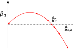
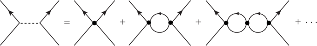
Figure 15: (Left) Schematic picture of the RG flow of the coupling constant for the four-fermion interaction $g_{s}$. The $\beta$ function crosses zero at $\hat{g}_{s}^{\ast}$. (Right) Bubble resummation for the four-fermion coupling $g_{s}$.

The physical interpretation of this condition (133) from the RG flow is quite informative (for a review, see Ref. [216]). For this purpose let us introduce the dimensionless coupling $\hat{g}_{s,k}\equiv g_{s,k}k^{2}$. The coupling constant in the NJL Lagrangian should be regarded as the bare one at the UV scale, i.e. $g_{s}=g_{s,\Lambda}$ at $k=\Lambda$. The $\beta$ function of $\hat{g}_{s,k}$ (denoted by $\beta_{g}$ here) behaves as shown schematically in the left panel of Fig. 15. If the dimensionless NJL coupling $\hat{g}_{s}$ is smaller than the fixed-point $\hat{g}_{s}^{\ast}$ that makes $\beta_{g}$ vanish, $\beta_{g}$ is positive and $\hat{g}_{s,k}$ goes smaller with decreasing $k$. If $\hat{g}_{s}$ is larger than $\hat{g}_{s}^{\ast}$, on the other hand, $\hat{g}_{s,k}$ gets larger and eventually diverges at $k\to 0$. This diverging behavior of $\hat{g}_{s,0}$ signals that chiral symmetry should be spontaneously broken. As a matter of fact, the RG flow is generated through the inclusion of fluctuations and $\hat{g}_{s,0}$ should contain all higher-loop diagrams in the four-fermion channel. In the one-loop order of $\beta_{g}$, after integrating with respect to $k$, $\hat{g}_{s,0}$ resums all bubble-type diagrams as sketched in the right panel of Fig. 15. Thus, there appear $\sigma$ and $\pi$ mesons in the intermediate states (dotted line in the right panel of Fig. 15) in $\hat{g}_{s,0}$, and $\hat{g}_{s,0}\to\infty$ at $k\to 0$ exactly corresponds to the (zero-momentum) propagation of massless mesons at the critical point. In this way, $g_{s}^{\ast}\Lambda^{2}$ in Eq. (133) can be given a clear interpretation.

With gauge field fluctuations, this $\beta_{g}$ is pushed down and if the gauge coupling is large enough, $\beta_{g}$ would be entirely negative, and chiral symmetry is spontaneously broken regardless of the starting point of the RG flow [216]. At finite temperate, on the other hand, $\beta_{g}$ is pushed up, and $\hat{g}_{s}^{\ast}$ moves toward a larger value. Then, when $\hat{g}_{s}^{\ast}$ becomes greater than a given $\hat{g}_{s}$ at a certain temperature, the second-order phase transition of chiral restoration occurs, as we see below.

Phase diagram in the mean-field approximation

At finite temperature and density the partition function of the quasi-particle excitations should be added to the thermodynamics potential, i.e.

$$\Omega_{\text{quark}}=-2N_{\text{c}}T\sum_{i}\int\frac{d^{3}p}{(2\pi)^{3}}\biggl{\{}\ln\bigl{[}1+e^{-(\varepsilon_{i}(p)-\mu_{\text{q}})/T}\bigr{]}+\ln\bigl{[}1+e^{-(\varepsilon_{i}(p)+\mu_{\text{q}})/T}\bigr{]}\biggr{\}}\;,$$ (134)

which induces a phase transition. In the chiral limit, again, we can find the critical temperature in the analytical way. That is, near the critical point, we can assume $T\gg M_{\text{q}}$ without loss of generality. Then, the high-$T$ expansion leads to,

$$\beta\Omega\simeq=-\frac{N_{\text{c}}N_{\text{f}}\Lambda^{4}}{4\pi^{2}}\biggl{\{}1+\Bigl{[}1-\frac{\pi^{2}}{N_{\text{c}}N_{\text{f}}g_{s}\Lambda^{2}}-\frac{\pi^{2}}{3}\Bigl{(}\frac{T}{\Lambda}\Bigr{)}^{2}-\Bigl{(}\frac{\mu_{\text{q}}}{\Lambda}\Bigr{)}^{2}\Bigr{]}\xi^{2}\biggr{\}}+\mathcal{O}(\xi^{4})\;.$$ (135)

The potential curvature has a modification from the finite-$T$ effects, and from the condition for the curvature to vanish at the critical point, the critical temperature is deduced as

$$T_{\text{c}}=\sqrt{\frac{3(\Lambda^{2}-\mu_{\text{q}}^{2})}{\pi^{2}}-\frac{3}{N_{\text{c}}N_{\text{f}}g_{s}}}\;.$$ (136)

This analytical result leads to a typical shape of the phase diagram in the $\mu_{\text{q}}$-$T$ plane as depicted in Fig. 16, where the Hatsuda-Kunihiro choice of the model parameters is used; $\Lambda=631\;\text{MeV}$ and $g_{s}=0.214\;\text{fm}^{2}$ for $N_{\text{f}}=2$.

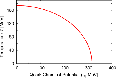
Figure 16: Typical shape of the phase diagram in the NJL model. The curve shows the analytical result (136) with $\Lambda=631\;\text{MeV}$ and $g_{s}=0.24\;\text{fm}^{2}$ used for the $N_{\text{f}}=2$ case.

So far, our discussions are limited to the special case of the second-order phase transition, and a possibility of the first-order phase transition cannot be ruled out from the above analysis. In fact, the phase diagram like the one presented in Fig. 16 should be more carefully examined and could be modified by a first-order phase boundary in the high-density region. This possibility and the underlying mechanism will be the subject of Sec. 4.3.

Coupling with the Polyakov loop

One of the major obstacles in the application of the NJL model to the finite-$T$ study is that this model may allow for unphysical quark excitations even below $T_{\text{c}}$. Such unphysical excitations should be diminished by the effect of confinement in reality. In other words, the thermal weight $e^{-(\varepsilon_{i}(p)\mp\mu_{\text{q}})/T}$ for quark excitations in Eq. (134) should be suppressed whenever the Polyakov loop $\Phi$ takes a small value. This can be easily implemented by the alteration of Eq. (134) into [217, 218]

$$\Omega_{\text{quark}} \to-2T\sum_{i}\int\frac{d^{3}p}{(2\pi)^{3}}\Bigl{\{}\text{tr}\ln\bigl{[}1+L\,e^{-(\varepsilon_{i}(p)-\mu_{\text{q}})/T}\bigr{]}+\text{tr}\ln\bigl{[}1+L^{\dagger}e^{-(\varepsilon_{i}(p)+\mu_{\text{q}})/T}\bigr{]}\Bigr{\}}\;.$$

$$=-2T\sum_{i}\int\frac{d^{3}p}{(2\pi)^{3}}\Bigl{\{}\ln\bigl{[}1+3\ell\,e^{-(\varepsilon_{i}(p)-\mu_{\text{q}})/T}+3\ell^{\ast}e^{-2(\varepsilon_{i}(p)-\mu_{\text{q}})/T}+e^{-3(\varepsilon_{i}(p)-\mu_{\text{q}})/T}\bigr{]}$$

$$\qquad\qquad\qquad\qquad\;+\ln\bigl{[}1+3\ell^{\ast}e^{-(\varepsilon_{i}(p)+\mu_{\text{q}})/T}+3\ell\,e^{-2(\varepsilon_{i}(p)+\mu_{\text{q}})/T}+e^{-3(\varepsilon_{i}(p)+\mu_{\text{q}})/T}\bigr{]}\Bigr{\}}\;.$$ (137)

In fact, in the field-theoretical derivation, one can arrive at the above coupling of Eq. (137) assuming that the Dirac operator has a constant $A_{4}$ background [218]. The integration along the temporal direction results in the Wilson line and thus the Polyakov loop as defined in Eq. (6).

This analytical structure itself is quite useful to understand some features of hot and dense QCD, especially the sign problem [38]. One can also find a reason why the strange quark (or heavy quark generally) number susceptibility can serve as a deconfinement order parameter. If the quark mass of the heavy flavor is sufficiently large, we can expand Eq. (137) and keep only the lowest-order term with respect to small Boltzmann weight. Then, differentiating the partition function with respect to the heavy-flavor chemical potential $\mu_{\text{s}}$ (which is eventually taken to be zero), we can derive the heavy-quark number $n_{\text{s}}\propto\langle\ell-\ell^{\ast}\rangle\,e^{-M_{\text{s}}/T}$ and the susceptibility $\chi_{\text{s}}\propto\langle\ell+\ell^{\ast}\rangle\,e^{-M_{\text{s}}/T}$. Since $\chi_{\text{s}}$ is proportional to the Polyakov loop, $\chi_{\text{s}}$ is qualified as an order parameter, which explains the right panel of Fig. 5.

To make concrete calculations, one needs to specify the effective potential for $\Phi$. Such a potential, $\Omega_{\text{glue}}[\Phi]$, is calculable in the perturbation theory that leads to what is called the Weiss potential [219, 220]. Non-perturbative evaluation is necessary, however, to describe a phase transition. The following Ansatz is well motivated from the strong-coupling expansion on the lattice;

$$\Omega_{\text{glue}}[\Phi]=-\frac{a(T)}{2}\bar{\Phi}\Phi+b(T)\ln\Bigl{[}1-6\bar{\Phi}\Phi+4(\bar{\Phi}^{3}+\Phi^{3})-3(\bar{\Phi}\Phi)^{2}\Bigr{]}\;,$$ (138)

where the logarithmic term has an origin in the Haar measure or the Jacobian associated with the variable change from $L$ to $A_{4}$. (The potential (138) is a function of the traced Polyakov loop that can be expressed using $A_{4}$, and thus the Jacobian from the group integration of $L$ to $A_{4}$ appears.) This Haar measure potential has cubic terms reflecting the color SU(3) nature. The $T$-dependent coefficients are chosen so that this $\Omega_{\text{glue}}[\Phi]$ can reproduce the thermodynamics of the pure Yang-Mills theory. One might wonder that $\Phi$ or $A_{4}$ cannot saturate the full thermodynamics and physical gluons should be rather two $A_{T}$’s (transverse components). The point is that $A_{T}$’s also couple to the Polyakov loop in the color adjoint representation and their thermal excitations can be controlled fully as a function of $\Phi$ [221, 222], which is also manifest in the non-perturbative construction of $\Omega_{\text{glue}}[\Phi]$ by means of the inverted Weiss potential [223, 224].

Suppose that $\Omega_{\text{glue}}[\Phi]$ is known, the Polyakov loop expectation value and the pressure are read from

$$\frac{\partial\Omega_{\text{glue}}[\bar{\Phi},\Phi]}{\partial\Phi}\biggr{|}_{\Phi=\Phi_{0},\bar{\Phi}=\bar{\Phi}_{0}}\!\!\!\!\!=\frac{\partial\Omega_{\text{glue}}[\bar{\Phi},\Phi]}{\partial\bar{\Phi}}\biggr{|}_{\Phi=\Phi_{0},\bar{\Phi}=\bar{\Phi}_{0}}\!\!\!\!\!=0\;,\qquad P=-\Omega_{\text{glue}}[\Phi_{0},\bar{\Phi}_{0}]/V\;.$$ (139)

We note that $\bar{\Phi}=\langle\ell^{\ast}\rangle$ is independent of $\Phi$ at finite density. For $\mu_{\text{q}}>0$ generally $\bar{\Phi}>\Phi$ is energetically favored. Once the expectation values $\bar{\Phi}_{0}$ and $\Phi_{0}$ are known, one can evaluate all other thermodynamic quantities from $\Omega_{\text{glue}}$. For the parametrization of $a(T)$ and $b(T)$ in Eq. (138) the following choice was inspired from the strong coupling expansion [225],

$$a(T)=12N_{\text{c}}^{2}\beta T\Lambda^{3}e^{-\alpha\Lambda/T}\;,\qquad b(T)=-\beta T\Lambda^{3}\;,$$ (140)

where $\alpha=1.052$ and $\beta=0.03$ are fixed to set the crossover temperature around $T=150\sim 200\;\text{MeV}$. Another frequently-used parametrization [226] is motivated to fit the thermodynamics of the pure Yang-Mills theory as

$$\frac{a(T)}{T^{4}}=3.51-2.47\biggl{(}\frac{T_{0}}{T}\biggr{)}+15.2\biggl{(}\frac{T_{0}}{T}\biggr{)}^{2}\;,\qquad\frac{b(T)}{T^{4}}=-1.75\biggl{(}\frac{T_{0}}{T}\biggr{)}^{3}$$ (141)

with $T_{0}$ being a scale parameter that characterizes the critical (crossover) temperature. Blue curves in Fig. 3 show a quantitative comparison between the lattice data and the potential fit from this $\Omega_{\text{glue}}$. The agreement is pretty good in the entire temperature range. One might have thought that the agreement is simply a result of the fit, but it is a highly non-trivial question whether the entire $T$ range can be covered with only three fitting parameters.

It is a straightforward extension of the NJL model with this modified $\Omega_{\text{quark}}$ of Eq. (137) and the Polyakov loop potential $\Omega_{\text{glue}}$ of Eq. (138). Such a model setup is called the Polyakov loop extended Nambu–Jona-Lasinio (PNJL) model (there are hundreds of application works; see e.g. Refs. [227]. Here let us make a technical remark; we still need to introduce a further approximation in the PNJL model for the treatment of Eq. (137). In many calculations the traced Polyakov loops are replaced as $\ell\to\Phi$ and $\ell^{\ast}\to\bar{\Phi}$, but this procedure assumes $\langle\ell^{n}\rangle\to\Phi^{n}$ and $\langle\ell^{\ast n}\rangle\to\bar{\Phi}^{n}$, which can be acceptable unless the Polyakov loop fluctuations become significant as compared to the expectation values. It is possible to go beyond this approximation to make use of a matrix model of the Polyakov loop [228, 229, 230].

Figure 17 shows typical results from the mean-field approximation of the (2+1)-flavor PNJL model. The order parameters, i.e. the Polyakov loop and the normalized chiral condensate are plotted as functions of $\mu_{\text{q}}$ and $T$. The NJL model parameters are fixed according to the Hatsuda-Kunihiro choice; $\Lambda=631\;\text{MeV}$, $m_{\text{u}}=m_{\text{d}}=5.5\;\text{MeV}$, $m_{\text{s}}=135.7\;\text{MeV}$, $g_{s}\Lambda^{2}=3.67$, $g_{d}\Lambda^{5}=-9.29$. In the market there are several different (and consistent) choices available; for example $\Lambda=602.3\;\text{MeV}$, $m_{\text{s}}=140.7\;\text{MeV}$, $g_{s}\Lambda^{2}=3.67$, $g_{d}\Lambda^{5}=-12.36$ [231] leading to qualitatively consistent results. We here make a remark that the PNJL model has been applied to color-superconductivity as well [226, 232], but one elaborates an improved treatment of the Polyakov loop [230], otherwise the color density behaves unphysically.

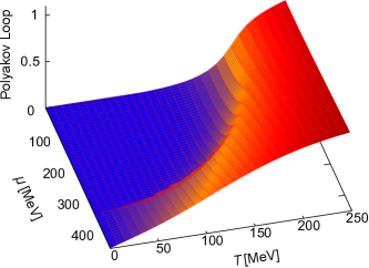
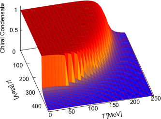
Figure 17: Order parameters calculated in the (2+1)-flavor PNJL model in the mean-field approximation. Figures adapted from Ref. [225].

We note that the trend of two simultaneous crossovers is semi-quantitatively reproduced in the whole $\mu_{\text{q}}$-$T$ region. There is seen a discontinuous jump in the chiral condensate in the high-density region, which signals a first-order phase transition. Actually it is quite non-trivial what is going on in the high-density region. One can see that the Polyakov loop stays small at low temperatures, though a jump is still visible which presumably arises from the mixing with the chiral condensate. One may be tempted to make a conclusion from the smallness of $\Phi$ that confinement must persist even in the high-density region. This smallness is intuitively understood from the interpretation of $\Phi$ as a single-quark free energy $f_{q}$, i.e., $\Phi\sim e^{-f_{q}/T}$. Quark confinement means $f_{q}\to\infty$ and so $\Phi\to 0$. However, even with a finite $f_{q}$, we can have $\Phi\to 0$ in the limit of $T\to 0$. Thus, $\Phi$ is no longer a good measure for deconfinement at low temperature. The physical picture of confinement and deconfinement of quarks still has subtleties, which has inspired theoretical deliberations on quarkyonic matter.

Finally, we make a remark on the sign problem within the framework of the PNJL model. The quasi-quark contribution of Eq. (137) corresponds to the logarithm of the Dirac determinant in the presence of constant $A_{0}$ from which $L$ and $L^{\dagger}$ emerge. In the color SU(3) case the traced Polyakov loops, $\ell$ and $\ell^{\ast}$, generally take a complex number. When the density is zero with $\mu_{\text{q}}=0$, the Dirac determinant is positive definite. At $\mu_{\text{q}}\neq 0$, however, $\Omega_{\text{quark}}$ can be complex, or its real-part can be negative. In the mean-field approximation in which $\text{tr}L$ and $\text{tr}L^{\dagger}$ are replaced with $\Phi$ and $\bar{\Phi}$, the energy becomes real and the sign problem seemingly disappears. However, we can show that the thermodynamic potential $\Omega[\Phi,\bar{\Phi}]$ is unstable in the direction of growing $\delta\Phi=\bar{\Phi}-\Phi$. The solution of the gap equation turns out to sit at the saddle point of the potential [233]. Such weird behavior of the thermodynamic potential is a manifestation of the difficulty of the sign problem within the mean-field approximation.

4.2.2 Quark-meson model

In the (P)NJL model it is technically complicated to include the effects of meson fluctuations. In such microscopic approaches the meson propagator is dynamically generated through quark loops, and thus, the momentum dependence is highly non-trivial. Moreover, the validity of the model is severely restricted by the Mott threshold for unphysical meson decay into a quark and an anti-quark.

Instead of the NJL model, depending on the problem, it would be sometimes more suitable to adopt another chiral model including meson degrees of freedom as point particles, namely, the linear sigma model. The linear sigma model usually has fermionic degrees of freedom as color-singlet baryons, but to investigate the phase transitions at high $T$ and/or $\mu_{\text{q}}$, quarks may be able to enter the dynamics, and then, a model with quarks and mesons could make more sense. Such a model setup with quarks and mesons is called the quark-meson (QM) model.

Problems in the mean-field approximation

In the two-flavor case, the QM model consists of quarks and light mesons, $\sigma$ and $\pi$, with the following Lagrangian density,

$$\mathcal{L}=\bar{\psi}\bigl{[}i\gamma_{\mu}\partial^{\mu}-g(\sigma+i\gamma_{5}\boldsymbol{\tau}\cdot\boldsymbol{\pi})\bigr{]}\psi+\frac{1}{2}(\partial_{\mu}\sigma)^{2}+\frac{1}{2}(\partial_{\mu}\vec{\pi})^{2}-\frac{\lambda}{4}(\sigma^{2}+\vec{\pi}^{2}-v^{2})^{2}+c\,\sigma\;.$$ (142)

With the potential in this Lagrangian density, chiral symmetry is spontaneously broken and the last term with $c=f_{\pi}m_{\pi}^{2}$ (which is constrained by the PCAC (23)) makes the potential slightly tilted so that $\sigma$ acquires an expectation value and three $\boldsymbol{\pi}$’s become the nearly massless NG bosons. In the chiral limit ($c=0$) one can perform the mean-field approximation simply in an analytical way, which is, however, troublesome as compared to the NJL model.

At $T=\mu_{\text{q}}=0$ the chiral symmetry breaking is almost trivial. The potential is so designed that $\sigma$ can have an expectation value at $v$, which turns out to be $f_{\pi}$. The constituent quark mass is then $M_{\text{q}}=g\sigma$. Unlike the NJL model the zero-point oscillation energy is discarded because the potential terms are supposed to take care of it. Then, at finite $T$, chiral restoration can be caused by meson excitations even without quarks, and this fact that one can treat meson loop effects is the advantage of the QM model over the NJL model. However, it is known that the simple mean-field approximation (or the Hartree approximation) would lead to an unphysical first-order phase transition due to the approximation artifact [234].

The presence of quarks would make the situation even worth. It is known by now that the conventional treatment of discarding Eq. (131) is inappropriate for the finite-$T$ investigation especially in the chiral limit [235]. To understand the problem, let us take a close look at Eq. (131). We have seen that this expanded form in terms of $\xi=M_{\text{q}}/\Lambda$ correctly describes a second-order phase transition in the NJL model. Strictly speaking, one should check if the quartic term $\sim\xi^{4}$ has a positive coefficient, and in the case of Eq. (131), indeed, the coefficient of the $\xi^{4}$ term has a logarithmic singularity $\sim-\ln|\sqrt{1+\xi^{2}}-1|\to+\infty$, and it is always positive for sufficiently small $\xi$. We note that this logarithmic singularity appears from the IR sector of massless quarks. Interestingly enough, at $T\neq 0$, this logarithmic singularity is exactly canceled by terms from Eq. (134) because quarks are fermions without Matsubara zero-mode at finite $T$. Therefore, the IR singularity should disappear whenever a finite $T$ is turned on. This implies that Eq. (134) alone without Eq. (131) would leave an uncanceled singularity, $+\ln|\sqrt{1+\xi^{2}}-1|\to-\infty$, for the coefficient of the $\xi^{4}$ term. So, a first-order phase transition occurs when the $\xi^{2}$-term approaches zero. This is obviously an artificial phase transition.

We can overcome this problem in the following way. One easy resolution is to introduce physical quark masses, and then the chiral phase transition is a smooth crossover. Such a treatment might be useful for qualitative studies at $\mu_{\text{q}}=0$, but the tendency to favor a first-order phase transition is overestimated, which is fatal for the QCD critical point search. For a more serious remedy, the latter problem is not so difficult to remove; because the logarithmic singularity is analytically known, one can cancel it by hand, or one can simply add the zero-point oscillation energy and readjust the model parameters. More cumbersome is the problem of artificial first-order transition; one should improve the approximation to go beyond the Hartree resummation.

Renormalization group improvement

It is a tedious calculation to handle the Fock and the higher-loop diagrams such as the sunset type [236]. Fortunately, nowadays, a sophisticated formulation for non-perturbative resummation has been developed well, which completely resolves the problem of artificial first-order phase transition.

Let us elaborate how to perform the calculation. The starting point is the functional RG equation, which is also known as the Wetterich equation [237], that is concisely written as

$$\frac{\partial\Gamma_{k}}{\partial k}=\frac{1}{2}\text{Tr}\bigl{(}R_{k}\,G_{k}\bigr{)}\;,\qquad G_{k\,ij}^{-1}(q)=\frac{\delta^{2}\Gamma_{k}}{\delta\phi_{i}(-q)\delta\phi_{j}(q)}+R_{k}(q)\delta_{ij}\;,$$ (143)

for generic scalar field theories. Here $i$, $j$ indicate the meson species such as $\sigma$ and $\pi$. The trace denoted by Tr involves the momentum integration as well as the sum over $i$, $j$. The scale $k$ refers to the RG scale and the effective action $\Gamma_{k}$ is coarse-grained up to this IR scale $k$. The important step to reach Eq. (143) is to introduce a scale-dependent mass that satisfies the following boundary condition,

$$R_{k}(q)\to\left\{\begin{array}[]{lp{1em}l}0&&(q^{2}\gg k^{2})\\ k^{2}&&(q^{2}\ll k^{2})\end{array}\right.\qquad\Longrightarrow\qquad\Gamma_{k}\to\left\{\begin{array}[]{lp{1em}l}\Gamma&&(k\to 0)\\ S&&(k=\Lambda)\end{array}\right.$$ (144)

Then, the theory has $k$-dependence through $R_{k}(q)$, and one can define the generating functional $Z_{k}[J]$, and $W_{k}[J]$ for connected diagrams in the standard method in the quantum field theory. The $k$-dependent effective action, $\Gamma_{k}[\phi]$, is a Legendre transform of $W_{k}[J]$. We note that the regulator term should be properly subtract by $-\frac{1}{2}\int d^{4}q\,R_{k}(q)\phi(-q)\phi(q)$ in the definition of $\Gamma_{k}[\phi]$ (see Ref. [238] for a pedagogical derivation). Since $R_{k}(q)$ vanishes in the limit of $k\to 0$, the coarse-grained action amounts to the standard effective action $\Gamma$ with full quantum effects, while $\Gamma_{k\to\Lambda}\to S$ where $S$ is the classical action and the flow start at the UV scale $\Lambda$. Actually Eq. (143) is the exact formula to define quantum field theories containing equivalent information as the functional quantization method. Therefore, of course, it is an impossible task to integrate Eq. (143) unless the theory is solvable.

A frequently-used assumption to go into the practical calculations is that the non-locality in the effective action is neglected so that $\Gamma_{k}[\phi]$ can be decomposed into the tree-level kinetic term and the local potential. Corresponding to the Lagrangian density of the QM model in Eq. (142) the Ansatz in this local potential approximation (LPA) is taken as

$$\Gamma_{k}[\sigma,\pi]=\int d^{4}x\biggl{\{}\bar{\psi}\bigl{[}i\gamma_{\mu}\partial^{\mu}-g(\sigma+i\gamma_{5}\boldsymbol{\tau}\cdot\boldsymbol{\pi})\bigr{]}\psi+\frac{1}{2}(\partial_{\mu}\sigma)^{2}+\frac{1}{2}(\partial_{\mu}\boldsymbol{\pi})^{2}+\Omega_{k}[\sigma,\pi]\biggr{\}}\;,$$ (145)

and then one can convert the RG equation for $\Gamma_{k}$ into that for $\Omega_{k}$. The RG equation turns out to be surprisingly simple under the choice of the so-called optimized regulator [239],

$$R_{k}(q)=(k^{2}-\boldsymbol{q}^{2})\theta(k^{2}-\boldsymbol{q}^{2})\;,$$ (146)

which is a useful choice for the finite-$T$ calculation, while the covariant form would be more appropriate for the $T=0$ case. One can immediately confirm that this simple choice satisfies the requirement (144). Thanks to the Heaviside theta function, one can carry the $q$-integration out analytically to find,

$$\frac{\partial\Omega_{k}}{\partial k}=\frac{k^{4}}{12\pi^{2}}\biggl{[}\frac{3}{E_{\pi}}\coth\Bigl{(}\frac{E_{\pi}}{2T}\Bigr{)}+\frac{1}{E_{\sigma}}\coth\Bigl{(}\frac{E_{\sigma}}{2T}\Bigr{)}-\frac{24}{E_{q}}\bigl{\{}1-n_{\text{F}}(E_{\text{q}}\!-\!\mu_{\text{q}})-n_{\text{F}}(E_{\text{q}}\!+\!\mu_{\text{q}})\bigr{\}}\biggr{]}\;,$$ (147)

where the quark part has a coefficient given by twice of the fermionic degrees of freedom, $2N_{\text{c}}N_{\text{f}}=12$. Here $n_{\text{F}}(E)$ is the Dirac-Fermi distribution function at $T$, and the energies in the denominator are $E_{i}=\sqrt{k^{2}+M_{i}^{2}}$ with

$$M_{\text{q}}^{2}=g^{2}\sigma^{2}\;,\qquad M_{\sigma}^{2}=\Omega_{k}^{\prime\prime}\;,\qquad M_{\pi}^{2}=\frac{\Omega_{k}^{\prime}}{\sigma}\;.$$ (148)

The $\sigma$ meson mass is naturally the curvature of the effective potential, and the pion mass is also the curvature with respect to the $\pi$ field, which can be expressed by the $\sigma$-derivative in an assumption that $\Omega_{k}$ is a function of $\sigma^{2}+\boldsymbol{\pi}^{2}$ (except for the explicit symmetry breaking term $c\sigma$).

There are two representative strategies to integrate the RG equation (147) with respect to $k$. One is to expand $\Omega_{k}(\sigma)$ around the minimum at each $k$. The whole shape of $\Omega_{k}(\sigma)$ is not necessary, but the meaningful observable is the potential value right at the physical point. Another method is to discretize $\Omega_{k}(\sigma)$ on the $\sigma$-grid and solve hundreds of differential equations numerically. In this latter formulation one does not have to find a minimum of the potential at each $k$.

We shall make some comments on the RG equation (143). In the traditional application of the RG analysis, the critical phenomena associated with the second-order phase transition have been of central interest and the critical exponents have been calculated around the IR fixed point. The applicability of the formula (143) is, however, not restricted only around the second-order phase transition. As we mentioned, Eq. (143) can be an alternative of the quantization scheme, and the full effective potential can be retrieved whether or not the system is far from the critical point. For the purpose to examine the first-order phase transition, the grid method is powerful enough to carve the double-well potential shape. In practical calculation, one should stop the $k$-integration at some small $k$ [60]; otherwise the potential becomes flat due to the convexity.

It is a straightforward extension of the QM model to introduce the coupling with the Polyakov loop in the same way as in Eq. (137), and this extended model is called the PQM model. In the PQM model the resulting phase diagram has turned out to be quite similar to what we have already discussed using the PNJL model. In particular chiral restoration in the high density region has a general tendency to favor the first-order phase transition. If the existence of the first-order boundary is a robust feature of the phase diagram, it ends up with a terminal that is to be identified as the second-order phase transition point. Then, around the critical region where fluctuations are enhanced, the (P)QM model should by far surpass the PNJL model. For the phase diagram and the critical properties around the QCD critical point in the PQM model, see Refs. [240, 241, 242, 243] and references therein. The question is, then, whether the first-order phase transition really exists or not.

4.3 Liquid-gas phase transition of quark matter

For the first-order phase transition at high density there is no universality argument. This is a dynamical problem depending on the details of the microscopic theory. Nevertheless, most of chiral models (without repulsive vector interactions) predict the first-order phase transition in the high-density region, and there must be some intuitive explanation for this general tendency [244, 245].

Let us start our heuristic argument with a simple setup; cold and dense quark matter in a quasi-particle description. This means that we assume a Fermi liquid of quark matter, which should be valid for bulk thermodynamic quantities as long as $T$ is small enough and the Landau damping is a minor effect. Then, the thermodynamic potential coming from a hot and dense medium is expressed as a function of the quasi-particle mass $M_{\text{q}}$ as

$$\Omega_{\text{matter}}(M_{\text{q}})=-\int_{0}^{\mu_{\text{q}}}d\mu^{\prime}\rho_{\text{q}}(\mu^{\prime})-4N_{\text{c}}N_{\text{f}}\,T\int\frac{d^{3}p}{(2\pi)^{3}}\ln\bigl{(}1+e^{-\omega_{p}/T}\bigr{)}\;,$$ (149)

where $\rho_{\text{q}}(\mu_{\text{q}})$ is the quark number density; $\rho_{\text{q}}(\mu_{\text{q}})=2N_{\text{c}}N_{\text{f}}\int\frac{d^{3}p}{(2\pi)^{3}}[n_{\text{F}}(\omega_{p}-\mu_{\text{q}})-n_{\text{F}}(\omega_{p}+\mu_{\text{q}})]$ and the dispersion relation is $\omega_{p}=\sqrt{p^{2}+M_{\text{q}}^{2}}$ in the quasi-particle picture. This form (149) is common in any chiral models such as the (P)NJL and the (P)QM models. It is then the vacuum part that is severely contaminated by model uncertainties.

In the spirit of the Ginzburg-Landau expansion, we can postulate the vacuum part as a polynomial form,

$$\Omega_{0}(M_{\text{q}})=a(M_{0}^{2}-M_{\text{q}}^{2})^{2}-bM_{\text{q}}-cM_{\text{q}}^{3}\;.$$ (150)

In the parametrization (150) $a$ is the curvature of the potential at the origin, $b$ represents the effect of the explicit symmetry breaking due to current quark mass, and $c$ takes care of the instanton-induced interaction for $N_{\text{f}}=3$. Here, for simplicity, we take $c=0$; we are interested in the reason why a first-order phase transition is dynamically favored at high density, and if $c\neq 0$ the tendency toward the first-order transition would be just strengthened by the tree-level contribution. The potential minimum is located around $M_{\text{q}}\simeq M_{0}$, so that $M_{0}$ is a parameter to be identified as the constituent quark mass in the vacuum.

Although this setup is extremely simple or even primitive, we emphasize that the above $\Omega_{0}+\Omega_{\text{matter}}$ can grasp the essential properties of all chiral quark models, except for the uncanceled logarithmic singularity in Eq. (149), which we will ignore here because it is dangerous only near the chiral limit. Moreover, in the regime at high $T$, meson fluctuations may give rise to $T$-dependent coefficients. Therefore, the analysis in this subsection is valid only for $\mu_{\text{q}}\gg T$.

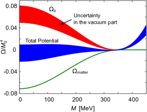
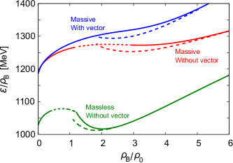
Figure 18: (Left) Potential shapes from Eqs. (149) and (150) at $T=0$ and $\mu_{\text{q}}=370\;\text{MeV}$. $\Omega_{\text{matter}}$ is fairly model independent, while uncertainty is unavoidable in $\Omega_{0}$. The parameters in $\Omega_{0}$ are chosen as $M_{0}=340\;\text{MeV}$, $a=0.05\sim 0.08$, $b=c=0$. (Right) The saturation curve of the energy per baryon as a function of the baryon density. From the bottom to the top, the solid curves represent the results in the chiral limit without the vector interaction, with massive quarks without the vector interaction, and with massive quarks with the vector interaction. The dotted parts are unstable and the dashed curves represent the branches corresponding to the chiral spiral. Figures adapted from Ref. [245].

The left panel of Fig. 18 shows the typical behavior of the effective potential. The matter part $\Omega_{\text{matter}}$ always has a minimum at $M_{\text{q}}=0$ because the baryon density is the largest when quasi-particles are massless. Then, together with $\Omega_{0}$ that has a minimum at $M_{\text{q}}=M_{0}$, it is conceivable to expect two minima in the total $\Omega$, and the absolute minimum jumps from one to the other at the first-order phase transition. This is the mechanism why the density effect tends to favor the first-order phase transition. At the same time, this argument can explain why the location and even the existence of the first-order boundary on the phase diagram are such model-dependent. The largest uncertainty comes from $a$; in Fig. 18 uncertainty associated with $a=0.05\sim 0.08$ (empirical values in the NJL and the QM models) is shown.

In the same way as the left panel of Fig. 7 for nuclear matter, it is useful to make a plot for the energy per baryon, $\varepsilon/\rho_{\rm B}$ at $T=0$, which is presented in the right panel of Fig. 18. As we already discussed in Sec. 3.1, the minimum of this curve tells us the saturation density and the binding energy. Because we are now working for quark matter, the saturation density can differ from $\rho_{0}$, and moreover, there may not be a minimum at all.

The existence of the first-order boundary of chiral restoration corresponds to the appearance of the minimum in the saturation curve. Thus, if quark droplets are possible [89], as is the case in Fig. 18 for massless $b=0$, the first-order phase transition and the QCD critical point can be concluded. From these analyses it is evident that the first-order phase transition in quark matter has exactly the same origin as the liquid-gas phase transition of nuclear matter. Even when droplets are only meta-stable, as is the case in Fig. 18 for $b=0.08M_{0}^{3}$ (massive, without vector), the first-order phase transition occurs.

We have not mentioned on the impact of the vector interaction as introduced in the Lagrangian density 124. The role of this type of the interaction is to add,

$$\Omega_{\text{vec}}(M_{\text{q}})=g_{v}\rho_{\text{q}}^{2}\;,$$ (151)

to the thermodynamic potential at the mean-field level. It should be noted that the mean-field calculation needs not only the tree-level $-g_{v}\rho_{\text{q}}^{2}$ term but also the shifted chemical potential $\mu_{\text{q}}^{\ast}$ as seen in Sec. 3.1.1. If expanded by the shift $g_{v}\rho_{\text{q}}$, this latter effect amounts to $2g_{v}\rho_{\text{q}}^{2}$, and Eq. (151) results together with the tree-level term.

It is obvious from the saturation curve that the repulsive ($g_{v}>0$) vector interaction always disfavors the first-order phase transition. The energy $\varepsilon$ is pushed up by $\propto\rho_{\rm B}^{2}$ from the vector interaction, and eventually the local minimum is completely washed out with increasing $g_{v}$, as exemplified in Fig. 18 for $b=0.08M_{0}^{3}$ and $g_{v}=0.12/M_{0}^{2}$ (massive, with vector). These parameters are arbitrarily chosen here for demonstration. Once the absence of the local minimum becomes the situation with sufficiently large $g_{v}$, there no longer appears a first-order phase boundary, and the QCD phase diagram has only smooth crossover entirely.

Above mentioned is the simplest and the most intuitive explanation about the impact of the vector interaction on the order of the chiral phase transition (at $T=0$) that was first addressed in a model study [246] and discussed repeatedly [225, 247, 248, 249]. See also Ref. [Lourenco:2012yv] for an attempt to estimate the strength of the vector interaction using the PNJL model.

4.4 Inhomogeneous chiral condensates

The existence of the QCD critical point is easily affected by unknown factors, while the inhomogeneous chiral condensate is more robust and, to the best of our knowledge, no counter-example against the inhomogeneous state has been found. Since the discovery of the relation between the QCD critical point and the Lifshitz point [250], more and more attention is being attracted to inhomogeneous quark matter, though there were earlier theoretical studies [251, 252, 253] and also the crystalline color-superconductors were intensely investigated in the higher density region (see Ref. [19] and references therein).

The simplest way to introduce inhomogeneity in the chiral condensate is to adopt the Ansatz of the chiral spiral, and actually, the chiral spiral is very useful to deepen the understanding of the driving force for spatial modulation. Under the 1-dimensional chiral-spiral Ansatz [254], the scalar and the pseudo-scalar condensates form a spiral (along the $z$-direction in our choice) as

$$\langle\bar{\psi}\psi\rangle=\chi\cos(2qz)\;,\qquad\langle\bar{\psi}\gamma_{5}\tau_{3}\psi\rangle=\chi\sin(2qz)$$ (152)

with a wave-number $q$. This is nothing but the quark-matter analogue of the $p$-wave pion condensation (117) in nuclear matter. Also, this Ansatz is sometimes referred to as the dual chiral-density wave [255].

The technical advantage of the chiral spiral is that this inhomogeneity is readily described by the redefinition of the basis; $\psi=e^{i\gamma_{5}\tau_{3}qz}\psi^{\prime}$ with a homogeneous condensate $\chi=\langle\bar{\psi}^{\prime}\psi^{\prime}\rangle$. Such a rotation in the chiral limit can remove the $\mu_{\text{q}}$-term in the Dirac operator, and then, the quasi-particle dispersion relation in the $\psi^{\prime}$-basis is expressed as

$$E_{p}=\sqrt{p_{\perp}^{2}+(\sqrt{p_{z}^{2}+M_{\text{q}}^{2}}\pm q)^{2}}$$ (153)

with dynamical mass $M_{\text{q}}$ on the $\psi^{\prime}$-basis. This type of simple inhomogeneity pattern has been considered repeatedly in various contexts such as large-$N_{\text{c}}$ QCD [256, 251], the Overhauser instability [252, 255], the quarkyonic chiral spiral [257], and so on. The dispersion relation (153) should be plugged into $\Omega_{\text{matter}}$ in Eq. (149) to evaluate the thermodynamic potential.

The most important observation is that a large part of the mass effect can be absorbed if $q\sim M_{\text{q}}$. Then, the density $\rho_{\text{q}}$ is not suppressed even with large $M_{\text{q}}$. In fact, the (1+1)-dimensional system is this extreme example; $\rho_{\text{q}}$ has an origin in the quantum anomaly and is completely insensitive to $M_{\text{q}}$ but dependent only on the chemical potential.

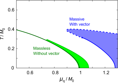
Figure 19: Typical phase diagrams with the chiral spiral for two cases. The solid curves represent a first-order phase transition. The shaded region in the left shows the chiral spiral for the massless ($b=0$) case without the vector interaction ($g_{v}=0$), and that in the right for the massive ($b=0.08M_{0}^{3}$) case with the vector interaction ($g_{v}=0.12/M_{0}^{2}$) with $M_{0}$ being a typical scale in the potential (150). Figure adapted from Ref. [245].

This simple observation from Eq. (153) can explain how the chiral spiral with $q\sim M_{\text{q}}$ can lower the total thermodynamic potential. If one makes a plot for $\Omega_{\text{matter}}(M_{\text{q}},q)$, one can find that this mechanism works efficiently and $\Omega_{\text{matter}}(M_{\text{q}},q)$ goes arbitrarily smaller for $q\sim M_{\text{q}}\to\infty$. This is a very simple and robust mechanism for the energy gain from finite $\vec{q}$. This large energy gain should overcome the energy loss from the kinetic term in $\Omega_{0}(M_{\text{q}},q)$, which can be expanded as

$$\Omega_{0}(M_{\text{q}},q)=\Omega_{0}(M_{\text{q}},q=0)+(\alpha M_{\text{q}}^{2}+\beta b)q^{2}\;.$$ (154)

The first term with $\alpha>0$ represents the kinetic term. One could estimate $\alpha$ using a chiral model, but one should be careful not to pick unphysical terms up from gauge-variant regularization. The term $\propto\beta$ is also necessary to take account of the effect of the current quark mass that would disfavor the chiral spiral. Quantitative details depend on $\alpha$ and $\beta$, but this setup with $\Omega_{0}(M_{\text{q}},q)+\Omega_{\text{matter}}(M_{\text{q}},q)$ suffices to capture the model-independent essence regardless of the choice of $\alpha$ and $\beta$.

Figure 19 shows typical phase diagrams resulting from this simple description with a choice, $\alpha=0.25$ and $\beta=0.25/M_{0}$. The chiral spiral is favored in the shaded region surrounded by the phase transitions of first order or second order.

We would stress that the vector interaction chosen here ($g_{v}=0.12/M_{0}^{2}$) is large enough to make the QCD critical point disappear from the phase diagram. Yet, the chiral spiral persists for any $g_{v}$ as confirmed in Fig. 19 even for the massive case with strong vector interaction. Therefore, the possibility of inhomogeneous states in quark matter is a more robust prediction from the model than the QCD critical point. The corresponding saturation curves are overlaid on the right panel of Fig. 18 with dashed lines. As noticed in this figure, it is possible that a local minimum is revived, so that a first-order phase boundary can come back with inclusion of the chiral spiral structure.

For more realistic ground states, it is desired to optimize the spatial structure beyond the Ansatz of the chiral spiral. This has been done by minimizing the Ginzburg-Landau potential and the solitonic solution is derived, which is known to have a lower energy than the chiral spiral in concrete model calculations [258, 259], which is also systematically investigated using the Ginzburg-Landau theory [260]. The saturation curves associated with such solitonic solutions are discussed in Ref. [261]. Even though the chiral spiral is an oversimplified form as compared to the soliton, it is still useful to exemplify that the inhomogeneous state takes over the homogeneous one. More theoretical studies are needed to clarify the stability of inhomogeneous states with other interactions (analogous to the effect of $g^{\prime}$ in the $p$-wave pion condensation) or with meson fluctuations in the RG method.

4.5 Quarkyonic matter

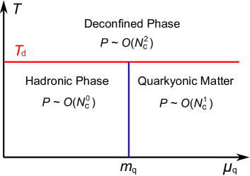
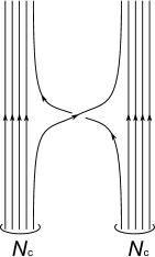
Figure 20: (Left) Schematic phase diagram of large-$N_{\text{c}}$ QCD.  The pressure is $\mathcal{O}(N_{\text{c}}^{0})$ in the hadronic phase, $\mathcal{O}(N_{\text{c}}^{2})$ in the deconfined phase, and $\mathcal{O}(N_{\text{c}}^{1})$ in quarkyonic matter. (Right) Baryon-baryon interaction of $\mathcal{O}(N_{\text{c}})$ in the large-$N_{\text{c}}$ limit. The exchanged quarks should have the same color. If they have the different color, one gluon exchange is necessary.

In the large-$N_{\text{c}}$ limit the deconfinement phase transition is well-defined and the phase structure associated with deconfinement is quite simple. As we have seen in Sec. 3.5 quark loops are suppressed by $1/N_{\text{c}}$ as compared to gluons, and yet, matter with finite baryon density may appear if the chemical potential is large enough. What does nuclear matter look like in the large-$N_{\text{c}}$ limit? We already have sufficient ingredients to tackle this question – we have discussed a Skyrme crystal in Sec. 3.5.2 and discovered a large-$N_{\text{c}}$ phase diagram in Fig. 14. We have also clarified the order parameter behavior in Fig. 17 obtained in the PNJL model in which the large-$N_{\text{c}}$ limit is implicitly assumed [262].

4.5.1 Phase diagram and the pressure

Apart from the fate of chiral symmetry, the phase diagram of large-$N_{\text{c}}$ QCD is as simple as in the left panel of Fig. 20, which is equivalent to Fig. 14 without a curve representing $T_{\chi}$. The horizontal line at $T=T_{\text{d}}$ is the deconfinement phase boundary below which only glueballs exist, the pressure of which should be of $\mathcal{O}(N_{\text{c}}^{0})$. Because there are $(N_{\text{c}}^{2}-1)$ gluons in the deconfined phase, the pressure sharply jumps from $\mathcal{O}(N_{\text{c}}^{0})$ in the glueball (or hadronic) phase to $\mathcal{O}(N_{\text{c}}^{2})$ in the deconfined phase. An onset for a finite quark density is located at $\mu_{\text{q}}=m_{\text{q}}$ and, if finite-density matter behaves as a free quark gas, its pressure is $\sim N_{\text{c}}\mu_{\text{q}}^{4}$. Hence, the deconfinement phase boundary cannot be affected by quarks unless $N_{\text{c}}\mu_{\text{q}}^{4}$ becomes comparable to $N_{\text{c}}^{2}$, namely, $\mu_{\text{q}}\sim\mathcal{O}(N_{\text{c}}^{1/4})$. Eventually, for $\mu_{\text{q}}\sim\mathcal{O}(N_{\text{c}}^{1/2})$, quarks are no longer suppressed by $1/N_{\text{c}}$ which is compensated by $\mu_{\text{q}}^{2}$ from the quark loop, and the gluon interactions are screened by dynamical quarks.

The above argument suggests that the pressure in the right-bottom part is of $\mathcal{O}(N_{\text{c}}^{1})$, which is indeed the case if the state of matter is a (nearly) free quark gas and $\mu_{\text{q}}\sim\mathcal{O}(N_{\text{c}}^{0})$. Such an argument is, however, too naïve; as is clear from Fig. 14 in the Sakai-Sugimoto model, the ground state in the low-$T$ and high-$\mu_{\text{q}}$ region is identified as nuclear matter rather than quark matter. This is also consistent with model studies as in Fig. 17 which implies quark confinement with small $\Phi$ in this region. In fact, gluons are confined below $T_{\text{d}}$, and it would be quite reasonable to assume that quarks are also confined there.

In Ref. [21] it was pointed out that the pressure of large-$N_{\text{c}}$ nuclear matter is of $\mathcal{O}(N_{\text{c}}^{1})$ and it resembles a pressure of quark matter. In nuclear matter at large $N_{\text{c}}$ nucleons are infinitely heavy and static, so that their kinetic energy is suppressed by $1/M_{\text{N}}\sim\mathcal{O}(N_{\text{c}}^{-1})$ and the dominant pressure contribution comes from the $NN$ interaction. Such a situation is correctly incorporated as a Skyrme crystal, which should be an approximate description of quarkyonic matter. Baryons at large $N_{\text{c}}$ interact strongly and the $NN$ interaction energy should be of $\mathcal{O}(N_{\text{c}})$, which is understood immediately from a diagram in the right panel of Fig. 20; the interaction is of order of the combinatorial factor to pick exchanged quarks up among $N_{\text{c}}$ quarks inside of baryon. One can make sure that not only the two-body but also the multi-baryon interactions generally scale as $\mathcal{O}(N_{\text{c}})$. In summary, in the large-$N_{\text{c}}$ limit, nuclear matter is a system of strongly interacting baryons, and it looks like knowing quark degrees of freedom in it. In Ref. [21] a name was given to such a baryonic and quark-like state of matter, i.e. quarkyonic matter.

If quarkyonic matter is a new state of matter, there must be some order parameter to characterize it. This is a natural question but is a source of confusion about the physical interpretation of quarkyonic matter. An intuitive picture of quarkyonic matter is the following; quarks deep inside the Fermi sphere are weakly interacting, because it is hard to excite these quarks above the Fermi sea due to Pauli blocking. On the other hand, the quarks near the Fermi surface with a shell-width $\sim\Lambda_{\text{QCD}}$ are not affected so much from the Pauli blocking and can interact strongly. Thus, the bulk thermodynamics such as the pressure, entropy and so on are dominated by the quarks inside of the Fermi sphere, while the physical excitations on top of the Fermi surface are dominated by color-singlet baryons.

4.5.2 Characterization of quarkyonic matter

A frequently-asked question is; what is the definition of quarkyonic matter? In other words, what is the order parameter for quarkyonic matter?

Formal definition

In accord with the original argument in Ref. [21], the definition of quarkyonic matter could be a state of matter that satisfies the McLerran-Pisarski conjecture. Here we introduced a term – the McLerran-Pisarski conjecture – which claims that a system of dense baryons be dual to a system of quarks. Thus, in quarkyonic matter, both descriptions of baryonic matter and quark matter can work to capture correct thermodynamic properties.

In Sec. 3.5.3 we mentioned on two density sources; the D4 instantons corresponding to baryons and the string sources corresponding to quarks in the Sakai-Sugimoto model. Although the baryonic state has a lower energy in the analysis in Ref. [22], such a treatment of the density sources may have some subtlety (for example the validity of the DBI action with a cusp singularity, see Ref. [263]). If the baryonic and quark sources turn out to be indistinguishable after all, it would be the clearest holographic example of quarkyonic matter.

Phenomenological signature

This above formal definition is not radical but quite understandable in view of the success of the thermal statistical model or the hadron resonance gas (HRG) model to capture the QCD thermodynamics [264]. (For details about the model setup, see Refs. [265, 266] and also Ref. [267] for a textbook.) In the HRG model it is assumed that hot and dense matter consists of non-interacting mesons, baryons, and all resonating states. This is a modern renovation of Hagedorn’s old idea (see Sec. 4.1). Suppose that all observed states obey the Hagedorn spectrum (122), the partition function blows up at $T=T_{\text{H}}$, and the growing behavior of the pressure near $T_{\text{c}}$ fits well with the one known from the lattice-QCD simulation as in Fig. 4. This observation is quite consistent with the behavior of QCD at large $N_{\text{c}}$. As we discussed in Sec. 3.5, the system is reduced to infinite towers of non-interacting mesons in the large-$N_{\text{c}}$ limit of QCD.

It is also known from the chiral effective models that the thermodynamic properties near $T_{\text{c}}$ are well understood in terms of quasi-quarks and gluons [224]. Therefore, thanks to a smooth crossover from the hadronic phase to the quark-gluon plasma, one can view the state of matter in this transitional region as both hadronic and quark-like. In a broad sense, the crossover region of QCD at zero density satisfies the McLerran-Pisarski conjecture, and the state of matter is quark-mesonic instead of quark-baryonic=quarkyonic.

In a narrow sense, quarkyonic matter should be distinguished from quark-mesonic matter. Baryons interact strongly, and this situation is so different from the description by the HRG model. In the thermal statistical model the interaction effects are indirectly taken into account via the Van der Waals force with a parameter of the excluded volume [268]. However, in physical processes, the interactions should encompass the quark degrees of freedom as depicted in the diagram of Fig. 20, and the excluded volume factor is not adequate to go into the regime of quarkyonic matter. Thus, in the beam-energy scan of the relativistic heavy-ion collision, if any deviation between the experimental data and the HRG model fit becomes more and more appreciable, it would hint quarkyonic matter.

Chiral property

Nuclear physicists would still wonder how quarkyonic matter can be different from ordinary nuclear matter in the real world with $N_{\text{c}}=3$. There is no clear-cut distinction. In nuclear matter $k_{\text{F}}$ is as small as the pion mass and the system is dilute (in a sense that one can perform the expansion with respect to $k_{\text{F}}$), while quarkyonic matter is dense by definition.

One possible characterization of quarkyonic matter is how it breaks chiral symmetry. In quarkyonic matter with infinitely large $N_{\text{c}}$ inhomogeneity is expected [251, 257]. This spatial modulation is attributed to the pseudo 1-dimensional nature on top of the Fermi surface at high density. Interestingly, as briefly noted in Sec. 3.5.3, the Sakai-Sugimoto model exhibits instabilities with respect to spatial modulations [197, 198]. However, this sort of inhomogeneity is nothing peculiar for nuclear physics; as addressed in Sec. 3.6, the $p$-wave pion condensation is essentially the same as the (quarkyonic) chiral spiral. Then, we have to conclude that quarkyonic matter is not really distinct from nuclear matter, or the $p$-wave pion condensation may be smoothly connected to the quarkyonic chiral spiral and vice versa.

4.5.3 Implications to the phase diagram

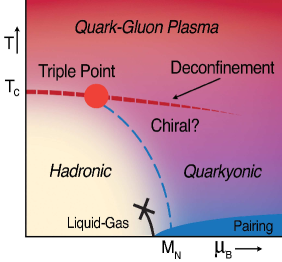
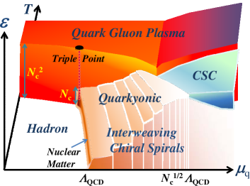
Figure 21: (Left) Phase diagram with a region that looks like a triple point where the hadronic phase, the deconfined phase (quark-gluon plasma), and quarkyonic matter meet. Figure adapted from Ref. [269]. (Right) Phase diagram with interweaving chiral spirals. Figure adapted from Ref. [270].

With quarkyonic matter in addition to the hadronic phase and the quark-gluon plasma, the phase diagram should take a structure of the left panel of Fig. 21, and then there may appear a region that looks like an approximate triple-point as speculated in Ref. [269] (see also the lattice-QCD results in Ref. [271]).

Later on, in Ref. [270], this phase diagram was brushed up into the form of the right panel of Fig. 21. Here the essential alteration is to add the phase structures associated with the quarkyonic chiral spirals. The chiral spiral is favored due to the pseudo 1-dimensionality, and the Fermi surface should be covered with such pseudo 1-dimensional patches. Because the transverse size of each patch is expected to be $\sim\Lambda_{\text{QCD}}$, the number of patches should increase with increasing $\mu_{\text{q}}$ (and increasing area of the Fermi surface). This “interweaving” picture naturally leads us to the speculation of successive phase transitions associated with the number of patches. In other words, the most optimal crystalline structure should depend on the density and the structural changes would divide the inhomogeneous region (as indicated by the shaded area in Fig. 19) into finer substates named the interweaving chiral spirals [270].

The most serious concern on reality of inhomogeneous quarkyonic matter is the validity of the extrapolation from $N_{\text{c}}=\infty$ to $N_{\text{c}}=3$, which is discussed for example in Ref. [272]. We finally point out that there exist quite a few theoretical arguments and pictures that are essentially indistinguishable from the McLerran-Pisarski conjecture and quarkyonic matter at $N_{\text{c}}=3$. A related duality (at zero density) has already been discussed in Ref. [273]. At high density the quark-hadron continuity in the context of color-superconductivity [274, 275] is not really different from the McLerran-Pisarski conjecture (for the confinement properties in color-superconductor, see Ref. [13]). At the phenomenological level the percolation model may provide us with an interpretation of quarkyonic matter at $N_{\text{c}}=3$ [276, 277].

5 Experimental Prospects

There are many theoretical speculations and conjectures on QCD at high density, and some of them should be filtered out by experimental data. Here we concisely discuss experimental implications to explore the properties of dense QCD matter.

5.1 Liquid-gas phase transition and the critical point

5.1.1 Experimental signals in nuclear matter

For general discussions on the liquid-gas phase transition, see Ref. [92] and references therein. Here we enumerate experimental signals for the critical point in nuclear matter. The extensive study of nuclear multi-fragmentation has been stimulated by the suggestion that this process might be a critical phenomenon [278, 279, 280, 281]. In particular the produced fragment distributions follow a power law of the form $P(A)\sim A^{-\tau}$ with the atomic number $A$, which suggests that a class of “universality” exists behind it [282]. Available multi-fragmentation data in nucleus-nucleus and hadron-nucleus reactions provide a distinct change of its character. Given these signals, the observation of the liquid-gas phase transition in a finite nuclear system is strongly supported [283, 284, 285, 286, 287].

The caloric curve, i.e. the heat versus temperature, is one of the important observables to distinguish the critical phenomena. Temperature of the system has to be reconstructed from observable quantities. In chemical and thermal equilibrium the temperature is extracted from the yields of isotope ratios [288]. The observed isotope temperature as a function of the excitation energy per nucleon $E/A$ shows a plateau over the range of relatively low $E/A$ [289, 290]. The observed caloric curve agrees qualitatively with predictions of the multi-fragmentation model [280] which is an event generator as a generalized liquid-drop model for hot nuclei, and the properties are consistent with a liquid-gas phase transition.

Another experimental signal of the phase transition is the appearance of a negative specific heat capacity: The entropy has typically a convex structure when a system experiences a first-order phase transition and this results in the specific heat $C$ being negative. This effect has been extracted from analysis of the energy fluctuations and the presence of a negative $C$ branch was indeed found [291].

The location of the critical point $T_{\text{c}}$ for the nuclear liquid-gas phase transition comes out from the observables. At this point the isotherm in the phase diagram has an inflection point. The major source of experimental information for $T_{\text{c}}$ is the fragment yield. However, the procedures to extract $T_{\text{c}}$ are highly scheme-dependent and the obtained values lie in a wide range $T_{\text{c}}\sim 5$-$20\;\text{MeV}$, indicating a severe model-dependence to be resolved (see e.g. Ref. [292]). The critical exponents have also been extracted from the moments of the fragmentation charge distributions [293, 294, 295]. The analysis concludes that the phase transition is of second order and finds the critical exponents consistent with the $\mathrm{Z}_{2}$ universality class.

5.1.2 Toward the QCD critical point

First-order phase transitions for cold and dense quark matter have been predicted in several approaches using chiral models [296, 297, 93], Dyson-Schwinger equations [298, 299, 300], and lattice-QCD in the strong coupling limit [301, 302, 303, 304, 305]. Given the observation of a crossover at zero chemical potential from lattice QCD computations, this might suggest an additional critical point other than that of the nuclear liquid-gas in the QCD phase diagram.

The order of the QCD phase transition at low temperature and high density is not established yet and thus the existence of a QCD critical point by itself remains an issue under debate. If it exists, the critical point must exhibit the critical exponents of the 3-dimensional Ising model that belongs to the $\mathrm{Z}_{2}$ universality class [306]. A potential signal for the QCD phase transition is modifications in the magnitude of fluctuations or the corresponding susceptibilities. In particular, fluctuations related to conserved quantities (baryon number $B$, quark number $q=3B$, electric charge $Q$, strangeness $S$, energy $E$, etc) play an important role since they are directly accessible in experiments [307].

A phase transition can be probed with response of a medium to temperature and chemical potential. The $n$-th order cumulant of a conserved quantity $X$, such as $B$, $q$, $Q$, $S$, etc, is computed from the partition function $Z$ via

$$\chi_{n}^{X}=\frac{1}{VT^{3}}\frac{\partial^{n}\ln Z}{\partial(\mu_{X}/T)^{n}}\;.$$ (155)

By taking the following cumulant ratios a volume factor can be eliminated;

$$R_{n,m}^{X}=\frac{\chi_{n}^{X}}{\chi_{m}^{X}}\;.$$ (156)

The ratios $R_{4,2}^{q}$ and $R_{4,2}^{Q}$ are shown to be sensitive to quark deconfinement at $\mu_{\text{q}}=0$ and they exhibit qualitatively different behavior from those of the HRG model [308]. At finite $\mu_{\text{q}}$ higher order cumulants of baryon number are particularly important since they diverge stronger on the chiral phase boundary in the chiral limit as well as at the critical point [309]. Higher moments and their signs have also been proposed as sensitive probes to the phase transitions [310].

Recently it has been shown that the fourth-order cumulant and the ratio $R_{4,2}$ (kurtosis) become universally negative when the critical point is approached from the crossover side [311]. Here the variance $\sigma_{X}$, the skewness $S_{X}$, and the kurtosis $\kappa_{X}$ are defined as

$$\sigma_{X}^{2}=VT^{3}\chi_{2}^{X}\;,\qquad S_{X}\sigma_{X}=\frac{\chi_{3}^{X}}{\chi_{2}^{X}}\;,\qquad\kappa_{X}\sigma_{X}^{2}=\frac{\chi_{4}^{X}}{\chi_{2}^{X}}\;.$$ (157)

A study using scaling functions shows that the fourth-order cumulant $\chi_{4}^{B}$ changes its sign around the crossover region from positive at lower temperature to negative at higher temperature, as a generic feature [312]. The temperature at which $\chi_{4}^{B}$ becomes negative is not universal since it depends on the regular part of the partition function. This suggests that the negative kurtosis is not a unique indicator of the critical point.

The STAR collaboration reported the ratio $R_{4,2}^{B}$ [313], which is consistent with the HRG model result [314, 315]. More recent data of the moment products, $\kappa_{X}\sigma_{X}^{2}$ and $S_{X}\sigma_{X}$, of the net proton number and electric charge distributions [316, 317, 318] differ from the HRG model result. This might be due to such simplified modeling of the QCD medium, although the thermal statistical model or the HRG model works well with various particle number ratios. So far, no experimental indication of the critical point is found.

If any signal of a first-order phase transition were observed, this would become an indication of the presence of the critical point as in the case of nuclear matter. In this respect, it is also challenging in heavy-ion collisions to observe the proposed consequences of the spinodal decomposition associated with a would-be first-order phase transition at high density, such as an enhancement of baryon and strangeness fluctuations [319, 320, 321] and a negative quark number susceptibility [322].

5.2 Dilepton measurements and chiral symmetry restoration

Dileptons are considered to be promising probes to study for changes of hadron properties in matter since they pass through the fireball created in heavy-ion collisions without hadronic interactions. The short-lived vector mesons like the $\rho$ mesons are expected to decay into dileptons inside the hot and dense matter. An enhancement in the dilepton rates below the $\rho/\omega$ resonance – indicating the medium modification of the vector mesons – has been observed in many experiments. Although a major number of experiments detected a strong width broadening and no “mass shift”, no perfect agreement among different experiments is reached yet [109, 323, 324]. A shift of the $\rho/\omega$ peak in the in-medium spectral function is often regarded as a “mass shift” of the vector meson. However, this is clearly an oversimplified interpretation since complicated reaction processes, numbers of resonances in a medium, and their interactions are involved and those complications are integrated into the final spectra. Therefore, picking up a maximum of such broad distributions does not readily give us the in-medium mass of the vector meson.

Below we will briefly argue some theoretical issues related to the dilepton measurements.

5.2.1 Is vector dominance fulfilled in a medium?

A lepton pair is emitted from the hot and dense matter through a decaying virtual photon. The differential production rate in the medium for fixed temperature $T$ or baryon density $\rho_{\rm B}$ is calculated with the imaginary part of the photon self-energy $\text{Im}\Pi$ via

$$\frac{dN}{d^{4}q}(q_{0},\vec{q};T,\rho_{\rm B})=\frac{\alpha^{2}}{\pi^{3}M^{2}}\,\frac{1}{e^{q_{0}/T}-1}\,\text{Im}\Pi(q_{0},\vec{q};T,\rho_{B})\;,$$ (158)

where $\alpha=e^{2}/4\pi$ is the electromagnetic coupling constant, $M$ is the invariant mass of the produced dilepton, and $q_{\mu}=(q_{0},\vec{q})$ denotes the momentum of the virtual photon. We will focus on an energy region around the $\rho$-meson mass scale in the following argument. In this energy range the photon self-energy is expected to be dominated by the two-pion process and its imaginary part is related to the pion electromagnetic form factor $\mathcal{F}(s;T)$ through

$$\text{Im}\Pi(s;T,\rho_{\rm B})=\frac{1}{6\pi\sqrt{s}}\biggl{(}\frac{s-4m_{\pi}^{2}}{4}\biggr{)}^{3/2}\bigl{|}\mathcal{F}(s;T,\rho_{\rm B})\bigr{|}^{2}$$ (159)

with the pion mass $m_{\pi}$ and the form factor given by

$$\mathcal{F}(s;T,\rho_{\rm B})=g_{\gamma\pi\pi}(T,\rho_{\rm B})+\frac{g_{\rho}(T,\rho_{\rm B})\cdot g_{\rho\pi\pi}(T,\rho_{\rm B})}{m_{\rho}^{2}(T,\rho_{\rm B})-s-\theta(s-4m_{\pi}^{2})\,im_{\rho}(T,\rho_{\rm B})\Gamma_{\rho}(s;T,\rho_{\rm B})}\;.$$ (160)

In matter-free space, a single photon mainly couples to two pions via the vector meson exchange, known as vector meson dominance (VD). This is assumed to hold in a hot and dense medium in many model calculations for the in-medium vector spectrum. One should, however, keep in mind that this is not a priori justifiable. A reliable theoretical framework to handle the VD is a hidden local symmetric (HLS) approach as discussed in Sec. 3.4; the vector meson properties are essentially controlled by one parameter $a$ and a particular choice, $a=2$, leads to vanishing photon-pion coupling,

$$g_{\gamma\pi\pi}(T=\rho_{\rm B}=0)=0\;.$$ (161)

A consistent achievement of chiral symmetry restoration at a given set of $T$ and $\rho_{\rm B}$ requires that the parameter $a$ should evolve toward unity with $T$ and $\rho_{\rm B}$ [325, 326, 327]. The immediate consequence is a strong violation of the VD in matter: The coupling $g_{\gamma\pi\pi}$ is an increasing function of thermal parameters whereas the vector-meson–photon coupling is a decreasing function of them toward chiral symmetry restoration as

$$g_{\gamma\pi\pi}\to\frac{1}{2}\;,\qquad g_{\rho}\to 0\;.$$ (162)

This indicates more dilepton rates from two-pion annihilation not involving the in-medium vector mesons when the system approaches the chiral phase transition. Thus the dilepton yields become suppressed there [328].

5.2.2 Has the BR scaling been excluded by the NA60 dimuon data?

The NA60 collaboration reported a strong in-medium broadening of the $\rho$ meson and no mass shift in dimuon measurements [329, 330]. The data were compared with the theoretical predictions based on phenomenological Lagrangians (width broadening due to hadronic many-body effects versus dropping $\rho$ mass), and the broadening with no mass shift is apparently favored. The measurement has excluded the scenario with a naïve dropping mass as in the form,

$$m_{\rho}(n)\sim m_{\rho}(n=0)\biggl{(}1-\alpha\frac{n}{n_{0}}\biggr{)}\;,$$ (163)

where $n$ represents either temperature or density, $\alpha$ a constant, and $n_{0}$ an appropriate scale for normalization.

If partial restoration of chiral symmetry modifies the vector meson property, it would appear not only in the mass but also all the interactions involving the vector meson. In principle those modifications should be incorporated systematically within a given effective theory for relevant hadrons. Therefore, a naïve replacement of the vector meson mass with Eq. (163) in the quantities such as the spectral function is incomplete. Also, the VD is shown to be violated at a certain $n$ once the vector meson, if its mass drops, feels partial chiral symmetry restoration [325, 326, 327]. On top of the in-medium broadening and the suppression of the vector-meson–photon coupling due to the VD violation, it was argued [331, 332, 167] that the signal of the Brown-Rho (BR) scaling is totally hidden in matter-free contributions essentially coming from the vector mesons which do not feel partial restoration and thus peaked around the vacuum mass, $m_{\rho}=770\;\text{MeV}$. Thus, a comparison of the data with the “dropping mass scenario” needs to be made with great caution.

Aiming to characterize a broad spectrum without clear resonance structure, an “average mass” can be introduced as [333, 334]

$$\bar{m}_{V,A}^{2}\equiv\frac{\int ds\,s\,\rho_{V,A}}{\int ds\,\rho_{V,A}}\;.$$ (164)

At order $T^{2}$ the vector meson pole mass does not receive any thermal corrections [335, 336] and the numerical analysis for $\bar{m}_{V}$ using QCD sum rules was shown to be consistent with this statement. The vector meson “mass” $\bar{m}_{V}$ stays almost constant up to $T\sim m_{\pi}$, whereas the axial-vector meson “mass” $\bar{m}_{A}$ decreases with rising temperature. Therefore, in this range of the temperature a dropping $\rho$ mass is not supported [334].

On the other hand, in-medium $\rho$ mesons in cold nuclear matter exhibit a different feature: The calculated $\bar{m}_{V}$ making use of the in-medium spectral function follows [333]

$$\frac{\bar{m}_{V}^{\ast}}{\bar{m}_{V}^{\rm vac}}\sim\frac{f_{\pi}^{\ast}}{f_{\pi}}\sim 1-0.15\,\frac{\rho_{\rm B}}{\rho_{0}}\;.$$ (165)

This suggests that the tendency of the BR scaling is indeed visible with the in-medium spectral function which shows a quite broad distribution. This observation is, contrary to the first impression, a good example of the “hidden” BR scaling in the broad spectrum in matter.

5.2.3 Chiral mixing in vector and axial-vector spectral functions

There is no doubt that dilepton measurements have observed in-medium modifications in the vector-meson channel. Yet, it remains unclear how such broadened vector spectra would eventually be linked to chiral symmetry restoration. Although the axial-vector spectral function is hardly measurable, axial-vector mesons come in to the vector spectrum via a mixing to pions in hot/nuclear matter [335, 337]. The mixing between the vector and axial-vector spectral functions, $\rho_{V}$ and $\rho_{A}$, is derived in a model-independent way at low $T$ and $\rho_{\rm B}$, arranged in a low-temperature/density theorem,

$$\begin{split}\rho_{V}(s;n)&=(1-\epsilon)\rho_{V}(s;0)+\epsilon\rho_{A}(s;0)\;,\\ \rho_{A}(s;n)&=(1-\epsilon)\rho_{A}(s;0)+\epsilon\rho_{V}(s;0)\;,\end{split}$$ (166)

where chiral mixing is characterized by the parameter $\epsilon=T^{2}/6f_{\pi}^{2}$ or $4\rho_{\rm B}\sigma_{\pi\text{N}}/3f_{\pi}^{2}m_{\pi}^{2}$ with the pion-nucleon sigma term $\sigma_{\pi\text{N}}$. The spectral functions with the mixing Eq. (166) at finite temperature has been explored in the QCD sum rules [338, 334, 339, 340] where one finds an indication of the expected tendency of the spectra $\rho_{V}$ and $\rho_{A}$ becoming degenerate.

Properties of the vector and axial-vector mesons constrained by current algebra are summarized in the sum rules for the spectral functions, known as Weinberg sum rules [175],

$$\int_{0}^{\infty}\frac{ds}{s}\bigl{[}\rho_{V}(s)-\rho_{A}(s)\bigr{]}=f_{\pi}^{2}\;,\qquad\int_{0}^{\infty}ds\bigl{[}\rho_{V}(s)-\rho_{A}(s)\bigr{]}=0\;.$$ (167)

Those sum rules extended to a finite temperature have been explored [341] where the following relation was deduced assuming the pole-saturated forms of $\rho_{V}$ and $\rho_{A}$;

$$\frac{f_{\pi}^{2}(T)}{f_{\pi}^{2}}=2Z_{\rho}(T)\biggl{(}\frac{m_{\rho}^{2}}{m_{\rho}^{2}(T)}-\frac{m_{\rho}^{2}}{m_{a_{1}}^{2}(T)}\biggr{)}$$ (168)

with the pole residue $Z_{\rho}$. Clearly, when $m_{\rho}(T)=m_{a_{1}}(T)$, chiral symmetry is restored with the vanishing order parameter $f_{\pi}(T)\to 0$. The sum rules by themselves do not distinguish how the masses behave with increasing temperature. Possible scenarios are (i) both decrease, (ii) both increase, (iii) $m_{\rho}(T)$ increases whereas $m_{a_{1}}(T)$ decreases. Using an $N_{f}=2$ linear sigma model, $m_{\rho}(T)$ is shown to go up by chiral restoration temperature if the VD holds in hot matter [342]. (See also Refs. [343, 344] for the linear sigma model with global chiral symmetry, which can be extended to non-zero temperature.) Non-linear sigma model calculations also yield the same tendency at low temperature where the VD is well satisfied [327]. If the VD is violated, there is no unique prediction unless one imposes a certain set of conditions for the model parameters being consistent with restoration of chiral symmetry.

The spectral functions $\rho_{V}$ and $\rho_{A}$ become degenerate when the mixing parameter reaches $\epsilon=1/2$. However, such a naïve extrapolation of Eq. (166) to higher $n$ requires the vector and axial-vector meson masses staying their vacuum values and thus they are not necessarily degenerate in contradiction to the desired property of chiral partners. An approach which does not rely on Eq. (166) is to use chiral effective theories of the vector and axial-vector mesons explicitly. The mixing and its evolution in matter are generated from processes involving the $\pi\,\rho\,a_{1}$ interaction. Due to the mixing the axial-vector meson appears as a bump in $\rho_{V}$ around $\sqrt{s}=m_{a_{1}}-m_{\pi}$ and this makes $\rho_{V}$ broadened. When the system evolves toward chiral symmetry restoration with temperature, it was shown that the chiral mixing vanishes at a critical point $T_{\text{c}}$ in the chiral limit [173]. Therefore the “maximal mixing” scenario, $\epsilon=1/2$, does not happen but instead, the resonance peak and the bump tend to be degenerate forming a single peaked structure which obviously indicating the degenerate $m_{\rho}$ and $m_{a_{1}}$. It is also interesting that even with explicit symmetry breaking the $\rho$ and $a_{1}$ masses are predicted to be well degenerate around a pseudo-critical temperature.

At finite chemical potential chiral mixing is generated at tree level since charge conjugation invariance is lost, which allows the following term that mixes vector and axial-vector fields [345],

$$\mathcal{L}_{\rm mix}=2C\epsilon^{0\nu\lambda\sigma}\text{tr}\bigl{[}\partial_{\nu}V_{\lambda}\cdot A_{\sigma}+\partial_{\nu}A_{\lambda}\cdot V_{\sigma}\bigr{]}$$ (169)

with the coupling $C$ and the total anti-symmetric tensor $\epsilon^{0123}=1$. One can deduce the above term from the $\omega\,\rho\,a_{1}$ part in the Wess-Zumino-Witten term with replacing $\omega_{0}$ with its expectation value,

$$\langle\omega_{0}\rangle=g_{\omega NN}\frac{\rho_{\rm B}}{m_{\omega}^{2}}\;.$$ (170)

Therefore, the coupling $C$ is

$$C=g_{\omega\rho a_{1}}\langle\omega_{0}\rangle\;,$$ (171)

and at normal nuclear density $\rho_{0}$ one finds $C\sim 0.1\;\text{GeV}$. The mixing term is also derived from the reduction of five-dimensional Chern-Simons action to four dimensions in a holographic QCD model [346] where $C\sim 1\;\text{GeV}$ at $\rho_{\rm B}=\rho_{0}$ was found. Such a strong mixing is, however, unrealistic since otherwise it yields vector meson condensation slightly above $\rho_{0}$. Thus, a large $C$ is supposed to be an artifact in large $N_{\text{c}}$ and/or of the specific model construction applied to a dense system.

The mixing term (169) modifies the dispersion relation resulting in

$$p_{0}^{2}-\vec{p}^{\;2}=\frac{1}{2}\biggl{[}m_{V}^{2}+m_{A}^{2}\pm\sqrt{(m_{A}^{2}-m_{V}^{2})^{2}+16C^{2}\vec{p}^{\;2}}\biggr{]}\;,$$ (172)

which describes the propagation of a mixture of the transverse $\rho$ and $a_{1}$ mesons. The longitudinal polarizations follow the standard dispersion relation. Consequently, the spin-averaged current correlator is superposition of the longitudinal mode peaked at $m_{V}$ and the transverse modes with two bumps peaked at shifted $m_{V}$ and $m_{A}$ obeying Eq. (172). The presence of mixing makes the entire spectral function broadened and this influences over dilepton production rates. Its impact on the rates crucially depends on the size of $C$. Let us suppose that the lowest $\omega$ dominance giving rise to $C\sim 0.1\;\text{GeV}$ at $\rho_{\rm B}=\rho_{0}$ is favored. Mixing does not have significance at this density. With increasing density, i.e. increasing $C$, the structure of the spectral function starts to show a change from the vacuum distribution, and such a modification becomes distinct when density reaches $\sim 3\rho_{0}$ [345].

The mixing (169) is chirally symmetric and thus does not vanish at chiral restoration in contrast to the vanishing chiral mixing at finite temperature without baryon density. In the presence of both mixing effects, a tendency of chiral symmetry restoration signaled by degenerating $\rho$ and $a_{1}$ mesons would become more obscure. Therefore, it seems a hard issue to observe a clear signal of chiral symmetry restoration in dilepton measurements. At least from the theoretical side, the in-medium vector spectral functions known to agree with data can be compared with the axial-vector spectra calculated in a given model with those mixing. Unless the description for the hadrons involved in terms of local fields breaks down totally, such a comparison could offer us an indirect evidence for the symmetry restoration, with attention to the notion of in-medium mass.

5.3 Astrophysical Implication

Historically speaking, the research on dense nuclear matter and the microscopic calculation of the EoS were motivated in the context of the structures of compact stellar objects (see e.g. Ref. [347] for a textbook).

There was an astonishing news in the year of 2010; it was reported in Ref. [25] that the Shapiro delay measurement for the binary pulsar PSR J1614-2230 results in the pulsar mass of $(1.97\pm 0.04)M_{\odot}$. This discovery has a tremendous impact on nuclear physics: Indeed, the abstract of Ref. [25] reads, “effectively rules out the presence of hyperons, bosons, or free quarks at densities comparable to the nuclear saturation density.” Once the EoS is known, one can plug $p(\rho)$, the pressure as a function of density, into the Tolman-Oppenheimer-Volkoff (TOV) equation to solve the relation between the mass and the radius of compact stars. The mass cannot be arbitrarily large but bounded by an upper limit corresponding to $p(\rho)$ that should sustain the star against the gravitational collapse. The EoS should be harder, i.e. $p$ should be larger for a given $\rho$, to support a larger mass.

The problem is that the EoS tends to be softer with exotic compositions, with which it may not be consistent with the existence of the neutron star as heavy as almost twice of the solar mass, though it can be; see Refs. [348, 349]. There is not really a final statement on this issue, and actually it is quite difficult to establish any reliable derivation of the EoS of quark matter (see e.g. Ref. [350] for a recent attempt), and thus it can become harder than believed (see Ref. [351] for example). Also, if the repulsive vector-interaction as in Eq. (124) is strong enough, it would easily make the EoS sufficiently hard. In other words, to explain the neutron star with $\sim 2M_{\odot}$, a substantially large vector interaction should be expected, and this implies in turn that the QCD critical point is disfavored from the QCD phase diagram [248].

Without assuming the state of matter, it is also a feasible program to compile astrophysical observations to constrain the EoS of dense matter directly. For recent progresses in this direction, see Refs. [352, 353, 354, 355].

The cooling rate is also informative on the state of matter in the neutron stars [356], and it is an interesting question how to constrain the possibility of the pion condensation [357]. We must keep in mind, however, that the environment of the neutron star is not necessarily the same as that we consider for the QCD phase diagram or for the heavy-ion collision. In the neutron star $\beta$ equilibrium is achieved, while it is usually symmetric nuclear and quark matter that is relevant to the phase diagram research. Besides, even if exotic contents such as the pion condensation, the kaon condensation, and quark matter were ruled out from the neutron-star observation (which is difficult from the mass-radius relation alone [348]), they might be still possible in symmetric matter and/or at higher densities.

6 Summary and Outlook

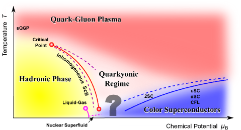
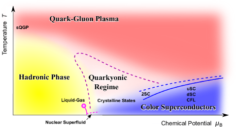
Figure 22: Two representative scenarios for the QCD phase diagram; one with the QCD critical point(s) adapted from Ref. [18] and the other without the first-order phase transition at all. “Quarkyonic Matter” is intentionally replaced with “Quarkyonic Regime” (see an explanation in the text).

In this review we have addressed physical properties of nuclear and quark matter and given pedagogical descriptions on the tools used in theoretical research. On the phase diagram with two environmental parameters, the temperature $T$ and the baryon chemical potential $\mu_{\text{B}}$, only a small portion has been understood; the QCD phase transitions of deconfinement and chiral restoration at (nearly) zero density, and the nuclear liquid-gas phase transition that is inevitable from the saturation property of nuclear matter. For the zero-density crossover, a pile of experimental and lattice-QCD data have been accumulated. Also the hadron resonance gas model works nicely, with which a physical picture has been established. In the nuclear physics territory the correct understanding is guided by experimental data, but the direct application of QCD to nuclear matter is still a big challenge. In practice one cannot avoid modeling the QCD dynamics in a form of the effective description.

In nuclear matter not far from the normal nuclear density chiral symmetry cannot be totally restored, but partial restoration has been confirmed both in theory and in experiment of the deeply bound pionic states. Mesons and baryons should be modified accordingly, and the hidden local symmetry model provides us with the most consistent description on these issues. It is, however, still hard to make conclusive statements on the changes of the hadron spectra and the mixing pattern at finite density. To grasp the qualitative character of dense matter, it is useful to increase the number of colors to infinity; $N_{\text{c}}\to\infty$. Then, the Skyrme model and also the most promising holographic QCD model (Sakai-Sugimoto model) tell us that the ground state of nuclear matter at $N_{\text{c}}\to\infty$ takes a crystal structure and spatial modulations should appear at high density, which is reminiscent of the old idea of the $p$-wave pion condensation.

Interestingly enough, this sort of inhomogeneity is favored by a robust mechanism in quark matter. Using a generic quasi-quark picture, we have demonstrated a simple calculation how the first-order phase transition and the inhomogeneous states can emerge in such a way induced by the density effects. This simple argument is helpful in understanding what part is robust and what part is not in theoretical predictions. We have demonstrated that the first-order phase transition and thus the QCD critical point can disappear from the phase diagram if the repulsive vector interaction is substantially strong, which is also suggested from the existence of the two-solar-mass neutron star. With the same parameter set, on the other hand, the inhomogeneous (chiral spiral) phase can persist, and we can say that the appearance of inhomogeneity is quite robust unlike the QCD critical point.

Then, it is conceivable that such inhomogeneous states of quark matter may be connected to the $p$-wave pion condensation. More generally, it might be even possible that strongly interacting nuclear matter has a dual description in terms of quark degrees of freedom. In fact, such “duality” is suggested in the large-$N_{\text{c}}$ counting, which defines a new regime on the phase diagram called quarkyonic matter. It was once said that quarkyonic matter could be a state with confinement but chiral symmetry restoration, but this characterization was misleading. The crucial aspects of quarkyonic matter are; (1) strong interaction of baryons, (2) inhomogeneous chiral condensates, and (3) quark degrees of freedom. Model buidling with these properties correctly equipped along the similar line to the hadron resonance gas model is an urgent theory problem.

What should the QCD phase diagram look like? In the market of the QCD phase diagram research, there are many variants of the schematic figures. We pick two representative scenarios up here in Fig. 22. The left figure (taken from Ref. [18]) is similar to the conventional type of the QCD phase diagram. It has a first-order boundary for the chiral phase transition and accommodates the critical point(s). The right one is a rather unconventional but these two phase diagrams are both viable enough. The QCD phase transitions, namely, deconfinement and chiral restoration, can be only crossovers and no critical point (apart from the nuclear liquid-gas transition) exists on the whole QCD phase diagram. Even in this case the inhomogeneous states around the regime of quarkyonic matter should be robust, as pictured with the dashed curve, in a sense that no model has falsified yet. In particular, in this latter scenario, the quarkyonic chiral spiral, the $p$-wave pion condensation in nuclear matter, and possibly the crystalline color-superconductivity may well be linked without sharp phase boundary, which is collectively referred to as “crystalline state” in the right panel of Fig. 22. In these figures we intentionally use a term “Quarkyonic Regime” instead of quarkyonic matter because it is important to note that quarkyonic matter is not a distinct state of matter. Quarkyonic matter should be understood as a transitional state between dense nuclear matter and quark matter, having both aspects of them.

With available theoretical knowledge and experimental data, it is still far from feasible to be able to select out the genuine one among many proposed diagram. We must solve QCD to establish a unique picture of the QCD phase diagram, and at the same time, we need more experimental data of the beam-energy scan from the relativistic heavy-ion collision. The sign problem inherent in the Monte-Carlo simulation is extraordinarily difficult to handle in a satisfactory manner, and the QCD phase diagram research awaits some other technical breakthrough not relying on the importance sampling.

As an extrapolation from nuclear matter toward higher density, one need to resort to effective approaches. Applying effective chiral Lagrangians in terms of a given set of mesons and baryons to dense matter is based on the assumption that those hadrons keep their particle identity and can still be expressed as local fields. It is not obvious whether this approximation is legitimate, but rather it can be taken as a working hypothesis. In fact, the spectroscopic factor for various nuclei indicating a deviation from the fully occupied mean-field orbits clearly shows that single-particle-ness of excitations reaches $\sim 70\%$ [358]. This would encourage modeling dense matter in a quasi-particle picture. In particular, when partial restoration of chiral symmetry sets in, light degree(s) of freedom that will be degenerate with the NG bosons must appear in a system. Thus, if one chooses “appropriate” degrees of freedom, such effective Lagrangian approaches with the local-field approximation would give a good description.

This speculative consideration is also supported by our knowledge on condensed matter physics where strongly correlated systems are well described by effective field theories and the notion of quasi-particles has been successful. A considerable example is a phase transition between the Néel (antiferromagnet) and valence bond solid (VBS, paramagnet) phases. Topology of those phases is well captured by the non-linear sigma models and a skyrmion configuration splitting into two half-skyrmions has been known [359, 360, 361]. The effective theory contains an emergent gauge field that mediates interactions between effective degrees of freedom [362]. This is quite suggestive and a similarity would be expected in nuclear many-body systems in high densities. Indeed, the concept of induced gauge fields, which arise when “fast” modes separated from “soft” modes are integrated out, have been recognized in various fields of physics [363]. In the context of QCD, non-Abelian gauge potentials (Berry phases) appear naturally in topological chiral bags under any adiabatic rotation [364].

On the QCD phase diagram we must widen our perspective outside of nuclear matter toward higher temperature and/or density, and the validity of effective approaches is questionable then. To this end, there is no bypass but solving QCD is the one-track way to reveal the QCD phase diagram completely. This used to be an impossible problem, but nowadays, it is becoming tractable owing to the technical developments in the functional methods. The QCD application of the Dyson-Schwinger equation has a long history and the mechanism of color confinement has been understood based on the gluon and the ghost propagators in the Landau gauge (see Ref. [365] for a review). Also, the Wetterich equation as we discussed in Sec. 4.2.2 is the exact formulation and has an equivalent content as the Dyson-Schwinger approach [366]. The QCD-based understanding of confinement is successfully transferred to the finite-$T$ studies on the QCD phase transitions [223, 367, 368, 369]. In these approaches toward QCD matter at high density, the most severe obstacle lies in the description of baryons and quarks on the equal footing. There is no model known in the market that can cope with baryons melting into quarks within a single framework. In principle, such a unified treatment of baryons and quarks may be formulated by means of dynamical hadronization with quarks and diquarks. Further progresses in the Dyson-Schwinger and the functional RG methods with inclusion of diquarks are indispensable for future studies.

The completion of the whole QCD phase diagram requires mutual collaborations extending over nuclear physics, high-energy particle physics and super-string theories, assisted by condensed-matter physics and astrophysics. This is such an interdisciplinary research area and new ideas are always desired.

References

- [1] N. Itoh, Prog. Theor. Phys. 44, 291 (1970).
- [2] J. C. Collins and M. J. Perry, Phys. Rev. Lett. 34, 1353 (1975).
- [3] J. Kapusta and C. Gale, Finite-Temperature Field Theory: Principles and Applications (Cambridge University Press, 2006).
- [4] M. Le Bellac, Thermal Field Theory (Cambridge University Press, 2000).
- [5] T. Appelquist and R. D. Pisarski, Phys. Rev. D23, 2305 (1981).
- [6] A. D. Linde, Rept. Prog. Phys. 42, 389 (1979).
- [7] A. D. Linde, Phys. Lett. B96, 289 (1980).
- [8] D. Zwanziger, Phys. Rev. D76, 125014 (2007), [hep-ph/0610021].
- [9] C. Manuel, Phys. Rev. D53, 5866 (1996), [hep-ph/9512365].
- [10] B. C. Barrois, Nucl. Phys. B129, 390 (1977).
- [11] D. Bailin and A. Love, Phys. Rept. 107, 325 (1984).
- [12] D. Son, Phys. Rev. D59, 094019 (1999), [hep-ph/9812287].
- [13] D. Rischke, D. Son and M. A. Stephanov, Phys. Rev. Lett. 87, 062001 (2001), [hep-ph/0011379].
- [14] M. G. Alford, K. Rajagopal and F. Wilczek, Phys. Lett. B422, 247 (1998), [hep-ph/9711395].
- [15] R. Rapp, T. Schafer, E. V. Shuryak and M. Velkovsky, Phys. Rev. Lett. 81, 53 (1998), [hep-ph/9711396].
- [16] M. G. Alford, A. Schmitt, K. Rajagopal and T. Schafer, Rev. Mod. Phys. 80, 1455 (2008), [0709.4635].
- [17] D. H. Rischke, Prog. Part. Nucl. Phys. 52, 197 (2004), [nucl-th/0305030].
- [18] K. Fukushima and T. Hatsuda, Rept. Prog. Phys. 74, 014001 (2011), [1005.4814].
- [19] R. Anglani et al., 1302.4264.
- [20] S. Muroya, A. Nakamura, C. Nonaka and T. Takaishi, Prog. Theor. Phys. 110, 615 (2003), [hep-lat/0306031].
- [21] L. McLerran and R. D. Pisarski, Nucl. Phys. A796, 83 (2007), [0706.2191].
- [22] O. Bergman, G. Lifschytz and M. Lippert, JHEP 0711, 056 (2007), [0708.0326].
- [23] T. Sakai and S. Sugimoto, Prog. Theor. Phys. 113, 843 (2005), [hep-th/0412141].
- [24] N. Cabibbo and G. Parisi, Phys. Lett. B59, 67 (1975).
- [25] P. Demorest, T. Pennucci, S. Ransom, M. Roberts and J. Hessels, Nature 467, 1081 (2010), [1010.5788].
- [26] M. A. Stephanov, Phys. Rev. Lett. 76, 4472 (1996), [hep-lat/9604003].
- [27] Particle Data Group, J. Beringer et al., Phys. Rev. D86, 010001 (2012).
- [28] C. Baker et al., Phys. Rev. Lett. 97, 131801 (2006), [hep-ex/0602020].
- [29] D. E. Kharzeev, L. D. McLerran and H. J. Warringa, Nucl. Phys. A803, 227 (2008), [0711.0950].
- [30] K. Fukushima, D. E. Kharzeev and H. J. Warringa, Phys. Rev. D78, 074033 (2008), [0808.3382].
- [31] E. Witten, Nucl. Phys. B156, 269 (1979).
- [32] G. Veneziano, Nucl. Phys. B159, 213 (1979).
- [33] S. Elitzur, Phys. Rev. D12, 3978 (1975).
- [34] F. Englert and R. Brout, Phys. Rev. Lett. 13, 321 (1964).
- [35] P. W. Higgs, Phys. Lett. 12, 132 (1964).
- [36] G. Guralnik, C. Hagen and T. Kibble, Phys. Rev. Lett. 13, 585 (1964).
- [37] K. James and P. Landshoff, Phys. Lett. B251, 167 (1990).
- [38] K. Fukushima, J. Phys. G39, 013101 (2012), [1108.2939].
- [39] A. V. Smilga, Phys. Rept. 291, 1 (1997), [hep-ph/9612347].
- [40] K. G. Wilson, Phys. Rev. D10, 2445 (1974).
- [41] C. E. Detar and L. D. McLerran, Phys. Lett. B119, 171 (1982).
- [42] H. Meyer-Ortmanns, Nucl. Phys. B230, 31 (1984).
- [43] R. D. Pisarski, Phys. Rev. D62, 111501 (2000), [hep-ph/0006205].
- [44] B. Svetitsky and L. G. Yaffe, Nucl. Phys. B210, 423 (1982).
- [45] B. Svetitsky, Phys. Rept. 132, 1 (1986).
- [46] J. Engels et al., Nucl. Phys. Proc. Suppl. 53, 420 (1997), [hep-lat/9608099].
- [47] P. de Forcrand and O. Jahn, Nucl. Phys. Proc. Suppl. 129, 709 (2004), [hep-lat/0309153].
- [48] J. Christensen, G. Thorleifsson, P. Damgaard and J. Wheater, Nucl. Phys. B374, 225 (1992).
- [49] B. Lucini, M. Teper and U. Wenger, JHEP 0401, 061 (2004), [hep-lat/0307017].
- [50] J. Engels, J. Fingberg and M. Weber, Nucl. Phys. B332, 737 (1990).
- [51] N. A. Alves, B. A. Berg and S. Sanielevici, Phys. Rev. Lett. 64, 3107 (1990).
- [52] C. Vafa and E. Witten, Phys. Rev. Lett. 53, 535 (1984).
- [53] J. B. Kogut and L. Susskind, Phys. Rev. D11, 3594 (1975).
- [54] G. ’t Hooft, Phys. Rev. Lett. 37, 8 (1976).
- [55] M. Kobayashi and T. Maskawa, Prog. Theor. Phys. 44, 1422 (1970).
- [56] R. Pisarski and L. Yaffe, Phys. Lett. B97, 110 (1980).
- [57] T. Schafer, Nucl. Phys. B575, 269 (2000), [hep-ph/9909574].
- [58] E. V. Shuryak, Comments Nucl. Part. Phys. 21, 235 (1994), [hep-ph/9310253].
- [59] R. D. Pisarski and F. Wilczek, Phys. Rev. D29, 338 (1984).
- [60] J. Berges, N. Tetradis and C. Wetterich, Phys. Lett. B393, 387 (1997), [hep-ph/9610354].
- [61] K. Fukushima, K. Kamikado and B. Klein, Phys. Rev. D83, 116005 (2011), [1010.6226].
- [62] Z. Fodor and S. Katz, 0908.3341.
- [63] O. Philipsen, 1207.5999.
- [64] S. Gupta, K. Huebner and O. Kaczmarek, Phys. Rev. D77, 034503 (2008), [0711.2251].
- [65] B. Beinlich, F. Karsch, E. Laermann and A. Peikert, Eur. Phys. J. C6, 133 (1999), [hep-lat/9707023].
- [66] S. Datta and S. Gupta, Phys. Rev. D82, 114505 (2010), [1006.0938].
- [67] M. Panero, Phys. Rev. Lett. 103, 232001 (2009), [0907.3719].
- [68] A. Mykkanen, M. Panero and K. Rummukainen, JHEP 1205, 069 (2012), [1202.2762].
- [69] S. Borsanyi, G. Endrodi, Z. Fodor, S. Katz and K. Szabo, JHEP 1207, 056 (2012), [1204.6184].
- [70] Y. Aoki, G. Endrodi, Z. Fodor, S. Katz and K. Szabo, Nature 443, 675 (2006), [hep-lat/0611014].
- [71] M. Cheng et al., Phys. Rev. D77, 014511 (2008), [0710.0354].
- [72] Wuppertal-Budapest Collaboration, S. Borsanyi et al., JHEP 1009, 073 (2010), [1005.3508].
- [73] S. Borsanyi et al., JHEP 1011, 077 (2010), [1007.2580].
- [74] Y. Hatta and K. Fukushima, Phys. Rev. D69, 097502 (2004), [hep-ph/0307068].
- [75] Y. Aoki, Z. Fodor, S. Katz and K. Szabo, Phys. Lett. B643, 46 (2006), [hep-lat/0609068].
- [76] A. Bazavov et al., Phys. Rev. D85, 054503 (2012), [1111.1710].
- [77] M. Cheng et al., Phys. Rev. D74, 054507 (2006), [hep-lat/0608013].
- [78] S. Ejiri et al., Phys. Rev. D80, 094505 (2009), [0909.5122].
- [79] O. Kaczmarek et al., Phys. Rev. D83, 014504 (2011), [1011.3130].
- [80] G. Endrodi, Z. Fodor, S. Katz and K. Szabo, JHEP 1104, 001 (2011), [1102.1356].
- [81] O. Philipsen, Prog. Theor. Phys. Suppl. 174, 206 (2008), [0808.0672].
- [82] S. Borsanyi et al., JHEP 1208, 053 (2012), [1204.6710].
- [83] E. Vicari and H. Panagopoulos, Phys. Rept. 470, 93 (2009), [0803.1593].
- [84] HotQCD Collaboration, A. Bazavov et al., Phys. Rev. D86, 094503 (2012), [1205.3535].
- [85] T. Csorgo, R. Vertesi and J. Sziklai, Phys. Rev. Lett. 105, 182301 (2010), [0912.5526].
- [86] N. Kaiser, S. Fritsch and W. Weise, Nucl. Phys. A697, 255 (2002), [nucl-th/0105057].
- [87] J. Walecka, Annals Phys. 83, 491 (1974).
- [88] S. Floerchinger and C. Wetterich, 1202.1671.
- [89] M. Buballa, Nucl.Phys. A611, 393 (1996), [nucl-th/9609044].
- [90] J. Boguta and A. Bodmer, Nucl. Phys. A292, 413 (1977).
- [91] S. Fiorilla, N. Kaiser and W. Weise, Nucl. Phys. A880, 65 (2012), [1111.2791].
- [92] T. Tatsumi, N. Yasutake and T. Maruyama, 1107.0804.
- [93] A. M. Halasz, A. Jackson, R. Shrock, M. A. Stephanov and J. Verbaarschot, Phys. Rev. D58, 096007 (1998), [hep-ph/9804290].
- [94] R. Haag, Phys. Rev. 112, 669 (1958).
- [95] J. Gasser, H. Leutwyler and M. Sainio, Phys. Lett. B253, 252 (1991).
- [96] J. Alarcon, J. Martin Camalich and J. Oller, Phys. Rev. D85, 051503 (2012), [1110.3797].
- [97] J. Gasser and H. Leutwyler, Phys. Lett. B184, 83 (1987).
- [98] P. Gerber and H. Leutwyler, Nucl. Phys. B321, 387 (1989).
- [99] K. Suzuki et al., Phys. Rev. Lett. 92, 072302 (2004), [nucl-ex/0211023].
- [100] S. Fiorilla, N. Kaiser and W. Weise, Prog. Part. Nucl. Phys. 67, 317 (2012), [1111.3688].
- [101] T. Becher and H. Leutwyler, Eur. Phys. J. C9, 643 (1999), [hep-ph/9901384].
- [102] T. Fuchs, J. Gegelia, G. Japaridze and S. Scherer, Phys. Rev. D68, 056005 (2003), [hep-ph/0302117].
- [103] E. E. Jenkins and A. V. Manohar, Phys. Lett. B255, 558 (1991).
- [104] V. Bernard, N. Kaiser, J. Kambor and U. G. Meissner, Nucl. Phys. B388, 315 (1992).
- [105] V. Bernard, N. Kaiser and U.-G. Meissner, Int. J. Mod. Phys. E4, 193 (1995), [hep-ph/9501384].
- [106] T.-S. Park, D.-P. Min and M. Rho, Phys. Rept. 233, 341 (1993), [hep-ph/9301295].
- [107] U. G. Meissner, J. A. Oller and A. Wirzba, Annals Phys. 297, 27 (2002), [nucl-th/0109026].
- [108] D. Jido, T. Hatsuda and T. Kunihiro, Phys. Lett. B670, 109 (2008), [0805.4453].
- [109] R. S. Hayano and T. Hatsuda, Rev. Mod. Phys. 82, 2949 (2010), [0812.1702].
- [110] S. Weinberg, Phys. Rev. 177, 2604 (1969).
- [111] S. Weinberg, Phys. Rev. Lett. 65, 1177 (1990).
- [112] F. J. Gilman and H. Harari, Phys. Rev. 165, 1803 (1968).
- [113] C. E. Detar and T. Kunihiro, Phys. Rev. D39, 2805 (1989).
- [114] Y. Nemoto, D. Jido, M. Oka and A. Hosaka, Phys. Rev. D57, 4124 (1998), [hep-ph/9710445].
- [115] S. Gallas, F. Giacosa and D. H. Rischke, Phys. Rev. D82, 014004 (2010), [0907.5084].
- [116] W.-G. Paeng, H. K. Lee, M. Rho and C. Sasaki, Phys. Rev. D85, 054022 (2012), [1109.5431].
- [117] T. Hatsuda and M. Prakash, Phys. Lett. B224, 11 (1989).
- [118] D. Zschiesche, L. Tolos, J. Schaffner-Bielich and R. D. Pisarski, Phys. Rev. C75, 055202 (2007), [nucl-th/0608044].
- [119] C. Sasaki and I. Mishustin, Phys. Rev. C82, 035204 (2010), [1005.4811].
- [120] S. Gallas, F. Giacosa and G. Pagliara, Nucl. Phys. A872, 13 (2011), [1105.5003].
- [121] C. Sasaki, H. K. Lee, W.-G. Paeng and M. Rho, Phys. Rev. D84, 034011 (2011), [1103.0184].
- [122] S. Weinberg, Phys. Rev. 166, 1568 (1968).
- [123] W. A. Bardeen, C. N. Leung and S. Love, Phys. Rev. Lett. 56, 1230 (1986).
- [124] G. Brown and M. Rho, Phys. Rev. Lett. 66, 2720 (1991).
- [125] M. Harada and C. Sasaki, Phys. Rev. D73, 036001 (2006), [hep-ph/0511312].
- [126] Y. Hidaka, O. Morimatsu and M. Ohtani, Phys. Rev. D73, 036004 (2006), [hep-ph/0512375].
- [127] J. Schechter, Phys. Rev. D21, 3393 (1980).
- [128] A. A. Migdal and M. A. Shifman, Phys. Lett. B114, 445 (1982).
- [129] A. Kerman and L. Miller, (1974).
- [130] R. Furnstahl, B. D. Serot and H.-B. Tang, Nucl. Phys. A598, 539 (1996), [nucl-th/9511028].
- [131] E. K. Heide, S. Rudaz and P. J. Ellis, Nucl. Phys. A571, 713 (1994), [nucl-th/9308002].
- [132] P. Papazoglou, S. Schramm, J. Schaffner-Bielich, H. Stoecker and W. Greiner, Phys. Rev. C57, 2576 (1998), [nucl-th/9706024].
- [133] V. Miransky and V. Gusynin, Prog. Theor. Phys. 81, 426 (1989).
- [134] R. Furnstahl, H.-B. Tang and B. D. Serot, Phys. Rev. C52, 1368 (1995), [hep-ph/9501386].
- [135] R. L. Jaffe, Phys. Rev. D15, 267 (1977).
- [136] R. L. Jaffe, Phys. Rev. D15, 281 (1977).
- [137] M. Knecht and J. Stern, hep-ph/9411253.
- [138] J. Stern, Phys. Rev. Lett. (1998), [hep-ph/9801282].
- [139] I. I. Kogan, A. Kovner and M. A. Shifman, Phys. Rev. D59, 016001 (1999), [hep-ph/9807286].
- [140] Y. Watanabe, K. Fukushima and T. Hatsuda, Prog. Theor. Phys. 111, 967 (2004), [hep-th/0312271].
- [141] M. Harada, C. Sasaki and S. Takemoto, Phys. Rev. D81, 016009 (2010), [0908.1361].
- [142] M. Bando, T. Kugo, S. Uehara, K. Yamawaki and T. Yanagida, Phys. Rev. Lett. 54, 1215 (1985).
- [143] M. Bando, T. Kugo and K. Yamawaki, Phys. Rept. 164, 217 (1988).
- [144] M. Harada and K. Yamawaki, Phys. Rept. 381, 1 (2003), [hep-ph/0302103].
- [145] T. Kugo, H. Terao and S. Uehara, (1985).
- [146] T. Kugo, Phys. Lett. B109, 205 (1982).
- [147] U. G. Meissner, Phys. Rept. 161, 213 (1988).
- [148] M. C. Birse, Z. Phys. A355, 231 (1996), [hep-ph/9603251].
- [149] M. Bando, T. Fujiwara and K. Yamawaki, Prog. Theor. Phys. 79, 1140 (1988).
- [150] N. Arkani-Hamed, A. G. Cohen and H. Georgi, Phys. Rev. Lett. 86, 4757 (2001), [hep-th/0104005].
- [151] N. Arkani-Hamed, A. G. Cohen and H. Georgi, Phys. Lett. B513, 232 (2001), [hep-ph/0105239].
- [152] N. Arkani-Hamed, H. Georgi and M. D. Schwartz, Annals Phys. 305, 96 (2003), [hep-th/0210184].
- [153] N. Arkani-Hamed, A. G. Cohen and H. Georgi, JHEP 0207, 020 (2002), [hep-th/0109082].
- [154] D. Son and M. Stephanov, Phys. Rev. D69, 065020 (2004), [hep-ph/0304182].
- [155] T. Sakai and S. Sugimoto, Prog. Theor. Phys. 114, 1083 (2005), [hep-th/0507073].
- [156] M. Harada, S. Matsuzaki and K. Yamawaki, Phys. Rev. D82, 076010 (2010), [1007.4715].
- [157] N. Seiberg, Nucl. Phys. B435, 129 (1995), [hep-th/9411149].
- [158] Z. Komargodski, JHEP 1102, 019 (2011), [1010.4105].
- [159] M. Harada and K. Yamawaki, Phys. Rev. Lett. 83, 3374 (1999), [hep-ph/9906445].
- [160] R. Kitano, JHEP 1111, 124 (2011), [1109.6158].
- [161] S. Abel and J. Barnard, JHEP 1205, 044 (2012), [1202.2863].
- [162] G. Brown and M. Rho, Phys. Rept. 269, 333 (1996), [hep-ph/9504250].
- [163] R. Furnstahl, B. D. Serot and H.-B. Tang, Nucl. Phys. A615, 441 (1997), [nucl-th/9608035].
- [164] B. D. Serot and J. D. Walecka, Int. J. Mod. Phys. E6, 515 (1997), [nucl-th/9701058].
- [165] R. Casalbuoni and R. Gatto, Phys. Lett. B464, 111 (1999), [hep-ph/9908227].
- [166] G. Brown and M. Rho, Phys. Rept. 363, 85 (2002), [hep-ph/0103102].
- [167] G. E. Brown, M. Harada, J. W. Holt, M. Rho and C. Sasaki, Prog. Theor. Phys. 121, 1209 (2009), [0901.1513].
- [168] M. Harada and K. Yamawaki, Phys. Lett. B297, 151 (1992), [hep-ph/9210208].
- [169] M. Tanabashi, Phys. Lett. B316, 534 (1993), [hep-ph/9306237].
- [170] H. Georgi, Phys. Rev. Lett. 63, 1917 (1989).
- [171] H. Georgi, Nucl. Phys. B331, 311 (1990).
- [172] M. Harada and K. Yamawaki, Phys. Rev. Lett. 86, 757 (2001), [hep-ph/0010207].
- [173] M. Harada, C. Sasaki and W. Weise, Phys. Rev. D78, 114003 (2008), [0807.1417].
- [174] S. Beane and U. van Kolck, Phys. Lett. B328, 137 (1994), [hep-ph/9401218].
- [175] S. Weinberg, Phys. Rev. Lett. 18, 507 (1967).
- [176] B. Lucini and M. Panero, 1210.4997.
- [177] G. ’t Hooft, Nucl. Phys. B72, 461 (1974).
- [178] E. Witten, Nucl. Phys. B160, 57 (1979).
- [179] M. Hanada and N. Yamamoto, JHEP 1202, 138 (2012), [1103.5480].
- [180] T. Skyrme, Nucl. Phys. 31, 556 (1962).
- [181] G. S. Adkins and C. R. Nappi, Phys. Lett. B137, 251 (1984).
- [182] I. R. Klebanov, Nucl. Phys. B262, 133 (1985).
- [183] K. Nawa, H. Suganuma and T. Kojo, Phys. Rev. D79, 026005 (2009), [0810.1005].
- [184] A. S. Goldhaber and N. Manton, Phys. Lett. B198, 231 (1987).
- [185] L. Castillejo, P. Jones, A. Jackson, J. Verbaarschot and A. Jackson, Nucl. Phys. A501, 801 (1989).
- [186] B.-Y. Park, D.-P. Min, M. Rho and V. Vento, Nucl. Phys. A707, 381 (2002), [nucl-th/0201014].
- [187] H.-J. Lee, B.-Y. Park, D.-P. Min, M. Rho and V. Vento, Nucl. Phys. A723, 427 (2003), [hep-ph/0302019].
- [188] M. Rho, S.-J. Sin and I. Zahed, Phys. Lett. B689, 23 (2010), [0910.3774].
- [189] K. Zarembo, JETP Lett. 75, 59 (2002), [hep-ph/0104305].
- [190] H. K. Lee, B.-Y. Park and M. Rho, Phys. Rev. C83, 025206 (2011), [1005.0255].
- [191] O. Aharony, S. S. Gubser, J. M. Maldacena, H. Ooguri and Y. Oz, Phys. Rept. 323, 183 (2000), [hep-th/9905111].
- [192] C. P. Herzog, Phys. Rev. Lett. 98, 091601 (2007), [hep-th/0608151].
- [193] G. Mandal and T. Morita, JHEP 1109, 073 (2011), [1107.4048].
- [194] E. Witten, JHEP 9807, 006 (1998), [hep-th/9805112].
- [195] O. Aharony, J. Sonnenschein and S. Yankielowicz, Annals Phys. 322, 1420 (2007), [hep-th/0604161].
- [196] Y. Kim, I. J. Shin and T. Tsukioka, 1205.4852.
- [197] W.-y. Chuang, S.-H. Dai, S. Kawamoto, F.-L. Lin and C.-P. Yeh, Phys. Rev. D83, 106003 (2011), [1004.0162].
- [198] H. Ooguri and C.-S. Park, Phys. Rev. Lett. 106, 061601 (2011), [1011.4144].
- [199] R. Sawyer and D. Scalapino, Phys. Rev. D7, 953 (1973).
- [200] A. Migdal, Phys. Rev. Lett. 31, 257 (1973).
- [201] R. Tamagaki, Prog. Theor. Phys. Suppl. 112, 1 (1993).
- [202] E. Oset, H. Toki and W. Weise, Phys. Rept. 83, 281 (1982).
- [203] E. Shiino, H. Toki, Y. Saito and M. Ichimura, Phys. Rev. C34, 1004 (1986).
- [204] T. Tatsumi, nucl-th/0302009.
- [205] R. Hagedorn, Nuovo Cim. Suppl. 3, 147 (1965).
- [206] K.-I. Kondo, Phys. Rev. D82, 065024 (2010), [1005.0314].
- [207] T. Hatsuda and T. Kunihiro, Phys. Rept. 247, 221 (1994), [hep-ph/9401310].
- [208] U. Vogl and W. Weise, Prog. Part. Nucl. Phys. 27, 195 (1991).
- [209] K. Kashiwa, H. Kouno, T. Sakaguchi, M. Matsuzaki and M. Yahiro, Phys. Lett. B647, 446 (2007), [nucl-th/0608078].
- [210] S. Schmidt, D. Blaschke and Y. Kalinovsky, Phys. Rev. C50, 435 (1994).
- [211] T. Hell, S. Roessner, M. Cristoforetti and W. Weise, Phys. Rev. D79, 014022 (2009), [0810.1099].
- [212] T. Hell, S. Rossner, M. Cristoforetti and W. Weise, Phys. Rev. D81, 074034 (2010), [0911.3510].
- [213] A. Radzhabov, D. Blaschke, M. Buballa and M. Volkov, Phys. Rev. D83, 116004 (2011), [1012.0664].
- [214] D. Horvatic, D. Blaschke, D. Klabucar and O. Kaczmarek, Phys. Rev. D84, 016005 (2011), [1012.2113].
- [215] Y. Nambu and G. Jona-Lasinio, Phys. Rev. 122, 345 (1961).
- [216] J. Braun, J. Phys. G39, 033001 (2012), [1108.4449].
- [217] K. Fukushima, Phys. Lett. B591, 277 (2004), [hep-ph/0310121].
- [218] C. Ratti, M. A. Thaler and W. Weise, Phys. Rev. D73, 014019 (2006), [hep-ph/0506234].
- [219] N. Weiss, Phys. Rev. D24, 475 (1981).
- [220] N. Weiss, Phys. Rev. D25, 2667 (1982).
- [221] K. Fukushima, Acta Phys. Polon. Supp. 3, 567 (2010).
- [222] C. Sasaki and K. Redlich, Phys. Rev. D86, 014007 (2012), [1204.4330].
- [223] J. Braun, H. Gies and J. M. Pawlowski, Phys. Lett. B684, 262 (2010), [0708.2413].
- [224] K. Fukushima and K. Kashiwa, 1206.0685.
- [225] K. Fukushima, Phys. Rev. D77, 114028 (2008), [0803.3318].
- [226] S. Roessner, C. Ratti and W. Weise, Phys. Rev. D75, 034007 (2007), [hep-ph/0609281].
- [227] D. Blaschke, M. Buballa, A. Radzhabov and M. Volkov, Yad.Fiz. 71, 2012 (2008), [0705.0384].
- [228] A. Dumitru, Y. Hatta, J. Lenaghan, K. Orginos and R. D. Pisarski, Phys. Rev. D70, 034511 (2004), [hep-th/0311223].
- [229] E. Megias, E. Ruiz Arriola and L. Salcedo, Phys. Rev. D74, 065005 (2006), [hep-ph/0412308].
- [230] H. Abuki and K. Fukushima, Phys. Lett. B676, 57 (2009), [0901.4821].
- [231] W.-j. Fu, Z. Zhang and Y.-x. Liu, Phys. Rev. D77, 014006 (2008), [0711.0154].
- [232] D. Gomez Dumm, D. Blaschke, A. Grunfeld and N. Scoccola, Phys. Rev. D78, 114021 (2008), [0807.1660].
- [233] K. Fukushima and Y. Hidaka, Phys. Rev. D75, 036002 (2007), [hep-ph/0610323].
- [234] G. Baym and G. Grinstein, Phys. Rev. D15, 2897 (1977).
- [235] V. Skokov, B. Friman, E. Nakano, K. Redlich and B.-J. Schaefer, Phys. Rev. D82, 034029 (2010), [1005.3166].
- [236] T. Nishikawa, O. Morimatsu and Y. Hidaka, Phys. Rev. D68, 076002 (2003), [hep-ph/0302098].
- [237] C. Wetterich, Phys. Lett. B301, 90 (1993).
- [238] J. Berges, hep-ph/9902419.
- [239] D. F. Litim, Phys. Lett. B486, 92 (2000), [hep-th/0005245].
- [240] B.-J. Schaefer, J. M. Pawlowski and J. Wambach, Phys. Rev. D76, 074023 (2007), [0704.3234].
- [241] B.-J. Schaefer, M. Wagner and J. Wambach, Phys. Rev. D81, 074013 (2010), [0910.5628].
- [242] B. Schaefer and M. Wagner, Phys. Rev. D85, 034027 (2012), [1111.6871].
- [243] T. K. Herbst, J. M. Pawlowski and B.-J. Schaefer, Phys. Lett. B696, 58 (2011), [1008.0081].
- [244] K. Fukushima, Phys. Rev. D78, 114019 (2008), [0809.3080].
- [245] K. Fukushima, Phys. Rev. D86, 054002 (2012), [1204.0594].
- [246] M. Kitazawa, T. Koide, T. Kunihiro and Y. Nemoto, Prog. Theor. Phys. 108, 929 (2002), [hep-ph/0207255].
- [247] C. Sasaki, B. Friman and K. Redlich, Phys. Rev. D75, 054026 (2007), [hep-ph/0611143].
- [248] N. M. Bratovic, T. Hatsuda and W. Weise, 1204.3788.
- [249] G. Contrera, A. Grunfeld and D. Blaschke, 1207.4890.
- [250] D. Nickel, Phys. Rev. Lett. 103, 072301 (2009), [0902.1778].
- [251] E. Shuster and D. Son, Nucl. Phys. B573, 434 (2000), [hep-ph/9905448].
- [252] B.-Y. Park, M. Rho, A. Wirzba and I. Zahed, Phys. Rev. D62, 034015 (2000), [hep-ph/9910347].
- [253] R. Rapp, E. V. Shuryak and I. Zahed, Phys. Rev. D63, 034008 (2001), [hep-ph/0008207].
- [254] V. Schon and M. Thies, hep-th/0008175.
- [255] E. Nakano and T. Tatsumi, Phys. Rev. D71, 114006 (2005), [hep-ph/0411350].
- [256] D. Deryagin, D. Y. Grigoriev and V. Rubakov, Int. J. Mod. Phys. A7, 659 (1992).
- [257] T. Kojo, Y. Hidaka, L. McLerran and R. D. Pisarski, Nucl. Phys. A843, 37 (2010), [0912.3800].
- [258] D. Nickel, Phys. Rev. D80, 074025 (2009), [0906.5295].
- [259] S. Carignano, D. Nickel and M. Buballa, Phys. Rev. D82, 054009 (2010), [1007.1397].
- [260] H. Abuki, D. Ishibashi and K. Suzuki, Phys. Rev. D85, 074002 (2012), [1109.1615].
- [261] M. Buballa and S. Carignano, 1210.7155.
- [262] L. McLerran, K. Redlich and C. Sasaki, Nucl. Phys. A824, 86 (2009), [0812.3585].
- [263] M. Harada, S. Nakamura and S. Takemoto, Phys. Rev. D86, 021901 (2012), [1112.2114].
- [264] A. Tawfik, Phys. Rev. D71, 054502 (2005), [hep-ph/0412336].
- [265] F. Becattini, J. Manninen and M. Gazdzicki, Phys. Rev. C73, 044905 (2006), [hep-ph/0511092].
- [266] A. Andronic, P. Braun-Munzinger and J. Stachel, Phys. Lett. B673, 142 (2009), [0812.1186].
- [267] J. Letessier and J. Rafelski, Hadrons and Quark-Gluon Plasma (Cambridge University Press, 2002).
- [268] A. Andronic, P. Braun-Munzinger, J. Stachel and M. Winn, Phys. Lett. B718, 80 (2012), [1201.0693].
- [269] A. Andronic et al., Nucl. Phys. A837, 65 (2010), [0911.4806].
- [270] T. Kojo, Y. Hidaka, K. Fukushima, L. D. McLerran and R. D. Pisarski, Nucl. Phys. A875, 94 (2012), [1107.2124].
- [271] Z. Fodor, S. D. Katz and C. Schmidt, JHEP 0703, 121 (2007), [hep-lat/0701022].
- [272] G. Torrieri and I. Mishustin, Phys. Rev. C82, 055202 (2010), [1006.2471].
- [273] C. Wetterich, Phys. Lett. B462, 164 (1999), [hep-th/9906062].
- [274] T. Schafer and F. Wilczek, Phys. Rev. Lett. 82, 3956 (1999), [hep-ph/9811473].
- [275] M. G. Alford, J. Berges and K. Rajagopal, Nucl. Phys. B558, 219 (1999), [hep-ph/9903502].
- [276] S. Lottini and G. Torrieri, Phys. Rev. Lett. 107, 152301 (2011), [1103.4824].
- [277] S. Lottini and G. Torrieri, 1204.3272.
- [278] J. Bondorf et al., Nucl. Phys. A443, 321 (1985).
- [279] J. Bondorf, R. Donangelo, I. Mishustin and H. Schulz, Nucl. Phys. A444, 460 (1985).
- [280] J. Bondorf, A. Botvina, A. Ilinov, I. Mishustin and K. Sneppen, Phys. Rept. 257, 133 (1995).
- [281] Y.-G. Ma, Phys. Rev. Lett. 83, 3617 (1999), [nucl-th/0102019].
- [282] J. Finn et al., Phys. Rev. Lett. 49, 1321 (1982).
- [283] A. Panagiotou, M. Curtin, H. Toki, D. Scott and P. Siemens, Phys. Rev. Lett. 52, 496 (1984).
- [284] V. Viola, Nucl. Phys. A734, 487 (2004), [nucl-ex/0311010].
- [285] V. Viola et al., Phys. Rept. 434, 1 (2006), [nucl-ex/0604012].
- [286] P. Chomaz, M. Colonna and J. Randrup, Phys. Rept. 389, 263 (2004).
- [287] Y. Ma et al., Phys. Rev. C71, 054606 (2005), [nucl-ex/0410018].
- [288] S. Albergo, S. Costa, E. Costanzo and A. Rubbino, Nuovo Cim. A89, 1 (1985).
- [289] J. Pochodzalla et al., Phys. Rev. Lett. 75, 1040 (1995).
- [290] J. Natowitz et al., Phys. Rev. C65, 034618 (2002), [nucl-ex/0106016].
- [291] M. D’Agostino et al., Phys. Lett. B473, 219 (2000), [nucl-ex/9906004].
- [292] V. Karnaukhov et al., Phys. Rev. C67, 011601 (2003), [nucl-ex/0302006].
- [293] J. Hufner, Phys. Rept. 125, 129 (1985).
- [294] EOS Collaboration, M. Gilkes et al., Phys. Rev. Lett. 73, 1590 (1994).
- [295] J. Elliott et al., Phys. Rev. C49, 3185 (1994).
- [296] M. Asakawa and K. Yazaki, Nucl. Phys. A504, 668 (1989).
- [297] J. Berges and K. Rajagopal, Nucl. Phys. B538, 215 (1999), [hep-ph/9804233].
- [298] A. Barducci, R. Casalbuoni, S. De Curtis, R. Gatto and G. Pettini, Phys. Lett. B231, 463 (1989).
- [299] A. Barducci, R. Casalbuoni, S. De Curtis, R. Gatto and G. Pettini, Phys. Rev. D41, 1610 (1990).
- [300] Y. Taniguchi and Y. Yoshida, Phys. Rev. D55, 2283 (1997), [hep-ph/9512375].
- [301] E.-M. Ilgenfritz and J. Kripfganz, Z. Phys. C29, 79 (1985).
- [302] P. Damgaard, D. Hochberg and N. Kawamoto, Phys. Lett. B158, 239 (1985).
- [303] F. Karsch and K. Mutter, Nucl. Phys. B313, 541 (1989).
- [304] K. Fukushima, Prog. Theor. Phys. Suppl. 153, 204 (2004), [hep-ph/0312057].
- [305] Y. Nishida, Phys. Rev. D69, 094501 (2004), [hep-ph/0312371].
- [306] F. Wilczek, Int. J. Mod. Phys. A7, 3911 (1992).
- [307] M. A. Stephanov, K. Rajagopal and E. V. Shuryak, Phys. Rev. Lett. 81, 4816 (1998), [hep-ph/9806219].
- [308] S. Ejiri, F. Karsch and K. Redlich, Phys. Lett. B633, 275 (2006), [hep-ph/0509051].
- [309] M. Stephanov, Phys. Rev. Lett. 102, 032301 (2009), [0809.3450].
- [310] M. Asakawa, S. Ejiri and M. Kitazawa, Phys. Rev. Lett. 103, 262301 (2009), [0904.2089].
- [311] M. Stephanov, Phys. Rev. Lett. 107, 052301 (2011), [1104.1627].
- [312] B. Friman, F. Karsch, K. Redlich and V. Skokov, Eur. Phys. J. C71, 1694 (2011), [1103.3511].
- [313] STAR Collaboration, M. Aggarwal et al., Phys. Rev. Lett. 105, 022302 (2010), [1004.4959].
- [314] F. Karsch and K. Redlich, Phys. Lett. B695, 136 (2011), [1007.2581].
- [315] R. Gavai and S. Gupta, Phys. Lett. B696, 459 (2011), [1001.3796].
- [316] STAR Collaboration, X. Luo, 1210.5573.
- [317] STAR Collaboration, D. McDonald, 1210.7023.
- [318] PHENIX Collaboration, J. Mitchell, 1211.6139.
- [319] D. Bower and S. Gavin, Heavy Ion Phys. 15, 269 (2002).
- [320] V. Koch, A. Majumder and J. Randrup, Phys. Rev. C72, 064903 (2005), [nucl-th/0509030].
- [321] J. Randrup, Phys. Rev. Lett. 92, 122301 (2004), [hep-ph/0308271].
- [322] C. Sasaki, B. Friman and K. Redlich, Phys. Rev. Lett. 99, 232301 (2007), [hep-ph/0702254].
- [323] S. Leupold, V. Metag and U. Mosel, Int. J. Mod. Phys. E19, 147 (2010), [0907.2388].
- [324] R. Rapp, J. Wambach and H. van Hees, 0901.3289.
- [325] M. Harada and C. Sasaki, Phys. Lett. B537, 280 (2002), [hep-ph/0109034].
- [326] M. Harada, Y. Kim and M. Rho, Phys. Rev. D66, 016003 (2002), [hep-ph/0111120].
- [327] M. Harada and C. Sasaki, Nucl. Phys. A736, 300 (2004), [hep-ph/0304282].
- [328] M. Harada and C. Sasaki, Phys. Rev. D74, 114006 (2006), [hep-ph/0608237].
- [329] NA60 Collaboration, R. Arnaldi et al., Phys. Rev. Lett. 96, 162302 (2006), [nucl-ex/0605007].
- [330] S. Damjanovic, Eur. Phys. J. C49, 235 (2007), [nucl-ex/0609026].
- [331] G. Brown and M. Rho, nucl-th/0509001.
- [332] G. Brown and M. Rho, nucl-th/0509002.
- [333] Y. Kwon, M. Procura and W. Weise, Phys. Rev. C78, 055203 (2008), [0803.3262].
- [334] Y. Kwon, C. Sasaki and W. Weise, Phys. Rev. C81, 065203 (2010), [1004.1059].
- [335] M. Dey, V. Eletsky and B. Ioffe, Phys. Lett. B252, 620 (1990).
- [336] V. Eletsky and B. Ioffe, Phys. Rev. D51, 2371 (1995), [hep-ph/9405371].
- [337] B. Krippa, Phys. Lett. B427, 13 (1998), [hep-ph/9708365].
- [338] E. Marco, R. Hofmann and W. Weise, Phys. Lett. B530, 88 (2002), [hep-ph/0110110].
- [339] P. M. Hohler and R. Rapp, Nucl. Phys. A892, 58 (2012), [1204.6309].
- [340] N. P. Holt, P. M. Hohler and R. Rapp, 1210.7210.
- [341] J. I. Kapusta and E. V. Shuryak, Phys. Rev. D49, 4694 (1994), [hep-ph/9312245].
- [342] R. D. Pisarski, Phys. Rev. D52, 3773 (1995), [hep-ph/9503328].
- [343] M. Urban, M. Buballa and J. Wambach, Nucl. Phys. A697, 338 (2002), [hep-ph/0102260].
- [344] D. Parganlija, F. Giacosa and D. H. Rischke, Phys. Rev. D82, 054024 (2010), [1003.4934].
- [345] M. Harada and C. Sasaki, Phys. Rev. C80, 054912 (2009), [0902.3608].
- [346] S. K. Domokos and J. A. Harvey, Phys. Rev. Lett. 99, 141602 (2007), [0704.1604].
- [347] S. Shapiro and S. Teukolsky, Black Holes, White Dwarfs and Neutron Stars (Wiley, 2008).
- [348] M. Alford, M. Braby, M. Paris and S. Reddy, Astrophys. J. 629, 969 (2005), [nucl-th/0411016].
- [349] T. Klahn et al., Phys.Lett. B654, 170 (2007), [nucl-th/0609067].
- [350] A. Kurkela, P. Romatschke and A. Vuorinen, Phys. Rev. D81, 105021 (2010), [0912.1856].
- [351] K. Masuda, T. Hatsuda and T. Takatsuka, 1205.3621.
- [352] F. Ozel, G. Baym and T. Guver, Phys. Rev. D82, 101301 (2010), [1002.3153].
- [353] J. M. Lattimer, Prog. Theor. Phys. Suppl. 186, 1 (2010).
- [354] H. Sotani, K. Nakazato, K. Iida and K. Oyamatsu, Phys. Rev. Lett. 108, 201101 (2012), [1202.6242].
- [355] A. W. Steiner, J. M. Lattimer and E. F. Brown, 1205.6871.
- [356] D. G. Yakovlev and C. Pethick, Ann. Rev. Astron. Astrophys. 42, 169 (2004), [astro-ph/0402143].
- [357] H. Umeda, K. Nomoto, S. Tsuruta, T. Muto and T. Tatsumi, Astrophys.J. 431, 309 (1994).
- [358] W. Dickhoff and C. Barbieri, Prog. Part. Nucl. Phys. 52, 377 (2004), [nucl-th/0402034].
- [359] F. Haldane, Phys. Rev. Lett. 61, 1029 (1988).
- [360] S. Chakravarty, B. I. Halperin and D. R. Nelson, Phys. Rev. B39, 2344 (1989).
- [361] N. Read and S. Sachdev, Phys. Rev. Lett. 62, 1694 (1989).
- [362] T. Senthil, A. Vishwanath, L. Balents, S. Sachdev and M. Fisher, SCIENCE 303, 1490 (2004).
- [363] E. Shapere, Alfred D. and E. Wilczek, Frank, Adv. Ser. Math. Phys. 5, 1 (1989).
- [364] H. Lee, M. A. Nowak, M. Rho and I. Zahed, Annals Phys. 227, 175 (1993), [hep-ph/9301242].
- [365] C. S. Fischer, A. Maas and J. M. Pawlowski, Annals Phys. 324, 2408 (2009), [0810.1987].
- [366] J. M. Pawlowski, D. F. Litim, S. Nedelko and L. von Smekal, Phys. Rev. Lett. 93, 152002 (2004), [hep-th/0312324].
- [367] J. Braun, L. M. Haas, F. Marhauser and J. M. Pawlowski, Phys. Rev. Lett. 106, 022002 (2011), [0908.0008].
- [368] C. S. Fischer, Phys. Rev. Lett. 103, 052003 (2009), [0904.2700].
- [369] C. S. Fischer, J. Luecker and J. A. Mueller, Phys. Lett. B702, 438 (2011), [1104.1564].