On estimating extremal dependence structures by parametric spectral measures

Abstract

Estimation of extreme value copulas is often required in situations where available data are sparse. Parametric methods may then be the preferred approach. A possible way of defining parametric families that are simple and, at the same time, cover a large variety of multivariate extremal dependence structures is to build models based on spectral measures. This approach is considered here. Parametric families of spectral measures are defined as convex hulls of suitable basis elements, and parameters are estimated by projecting an initial nonparametric estimator on these finite-dimensional spaces. Asymptotic distributions are derived for the estimated parameters and the resulting estimates of the spectral measure and the extreme value copula. Finite sample properties are illustrated by a simulation study.

1 Introduction

Extreme value copulas provide a suitable general approach to modelling multivariate extremes. Various nonparametric methods for estimating extreme value copulas have been proposed in the last few years [17], [10], [11], [3] (also see [15], [5] and [13] for related approaches). In practical applications, such as for instance operational risk or rare natural disasters, one is however often in a situation where available data are sparse. Nonparametric methods generally require a fairly large sample size in order to be reliable. For small samples and in situations where one may have some idea about plausible properties of the distribution, parametric methods are likely to yield more accurate results. An approach to parametric inference for extreme value copulas is discussed for instance in [2].

One of the key issues is how to define parametric families that are simple and at the same time general enough to cover a large variety of multivariate dependence structures in the extremes. For instance, some of the most popular models are based on Archimedean copulas, which all correspond to the same type of extremal dependence structure, characterized by the Gumbel copula [7]. One way of achieving more flexibility in the extremes is to build models based on spectral measures. This is the approach taken here. For related work see e.g. [6], [12], and [11].

More specifically, the idea pursued in the following is to select a finite number of suitable spectral measures as basis elements and to use their convex combinations as a parametric family of dependence structures. Given a sufficiently large number of such basis elements, any spectral measure can be approximated by a weighted sum. Estimation of the coefficients can then be carried out by projecting a nonparametric estimator, such as the one in [3], on the finite-dimensional space generated by the basis elements. If the number of basis elements in the model is large (and increasing with the sample size), then projecting the original non-parametric estimator can be considered as a discretization technique. This is the setting in [6] and [11].

On the other hand, an appropriate model with a small number of basis elements can have the advantage of dimension reduction. Given a reasonable parametric model with a small number of parameters, one can reduce the variability of a nonparametric estimator by projecting it on a low-dimensional space. This is the approach studied here. We define explicit parameter estimators in the low-dimensional setting and study the asymptotic distribution of the resulting estimators of the dependence structure. To illustrate the potential advantage of dimension reduction, we construct an example with three basis elements and compare a non-parametric estimator with its low-dimensional projection in a simulation study.

Note that in principle any nonparametric estimator (cf. [5], [3], [13], [17], [10], [11]) can be used as a starting point. Depending on the nonparametric method used in the projection, the marginal distributions are either known or estimated from the observed data. The asymptotic results given below only require that a functional limit theorem in a suitable topology holds for the initial estimator.

The paper is organized as follows. Basic definitions and concepts of multivariate extreme value theory are summarized in section 2. Parametric models in the spectral domain and a corresponding parametric estimator are introduced in section 3. Asymptotic results, including consistency and a central limit theorem, are derived in section 4. The theoretical results are illustrated by simulations for a specific model in section 5. Final remarks in section 6 with a discussion of some open problems conclude the paper.

2 Basic definitions

Consider a sample $\mathbf{X}_{1},\ldots,\mathbf{X}_{n}$ consisting of iid realizations $\mathbf{X}_{i}=\left(X_{i,1},\ldots,X_{i,d}\right)^{T}$ of a $d$-dimensional random vector $\mathbf{X}=\left(X_{1},\ldots,X_{d}\right)^{T}\in\mathbb{R}^{d}$ with marginal distributions $F_{1},\ldots,F_{d}$ and copula $C_{\mathbf{X}}$. That is, $F_{j}(t)=P\left(X_{j}\leq t\right)$ for $j=1,\ldots,d$ and $t\in\mathbb{R}$, and

$$P\left(\mathbf{X}\leq\mathbf{x}\right)=C_{\mathbf{X}}\left(F_{1}\left(x_{1}\right),\ldots,F_{d}\left(x_{d}\right)\right)$$

for $\mathbf{x}\in\mathbb{R}^{d}$. The notation $\mathbf{x}\leq\mathbf{y}$ for $\mathbf{x},\mathbf{y}\in\mathbb{R}^{d}$ means $x_{j}\leq y_{j}$ for $j=1,\ldots,d$. The transposition operator $(\cdot)^{T}$ in $\mathbf{X}=\left(X_{1},\ldots,X_{d}\right)^{T}$ indicates that $\mathbf{X}$ is considered as a column vector. Distinguishing columns and rows will be useful in some calculations later on.

The vector $\mathbf{M}_{n}=\left(M_{n,1},\ldots,M_{n,d}\right)^{T}$ of componentwise maxima

$$M_{n,j}=\max_{i=1,2,\ldots,n}X_{i,j}$$

then has marginal distributions $P(M_{n,j}\leq t)=F_{j}^{n}(t)$ and a copula $C_{\mathbf{M}_{n}}\left(u\right)$ given by

$$P\left(\mathbf{M}_{n}\leq\mathbf{x}\right)=C_{\mathbf{M}_{n}}\left(F_{1}^{n}\left(x_{1}\right),\ldots,F_{d}^{n}\left(x_{d}\right)\right)=C_{\mathbf{X}}^{n}\left(F_{1}\left(x_{1}\right),\ldots,F_{d}\left(x_{d}\right)\right).$$

In the limit one obtains, under general conditions, an extreme value copula $C\left(\mathbf{u}\right)=\lim_{n\rightarrow\infty}C_{\mathbf{X}}^{n}\left(\mathbf{u}^{1/n}\right)$ ($\mathbf{u}=\left(u_{1},\ldots,u_{d}\right)^{T}\in\left[0,1\right]^{d}$) with the characteristic max-stable property

$$C\left(\mathbf{u}\right)=C^{n}\left(\mathbf{u}^{1/n}\right)$$ (1)

for all $n\in\mathbb{N}$. For an accessible introduction to this topic see e.g. [9] and references therein. The definition (1) of extreme value or max-stable copulas is equivalent to the representation

$$C\left(\mathbf{u}\right)=\exp\left(-\ell\left(-\log u_{1},\ldots,-\log u_{d}\right)\right)$$

with the tail dependence function

$$\ell(\mathbf{x})=\int_{\Delta_{d}}\max_{i=1,\ldots,d}\left(w_{i}x_{i}\right)d\Psi\left(w_{1},\ldots,w_{d}\right),\quad(\mathbf{x}\in[0,\infty)^{d}),$$ (2)

and $\Psi$ the so-called spectral measure on the unit simplex in $\mathbb{R}^{d}$, $\Delta_{d}=\{\mathbf{x}\in[0,1]^{d}:\sum_{i=1}^{d}x_{i}=1\}$, satisfying

$$\int_{\Delta_{d}}w_{i}d\Psi(w_{1},\ldots,w_{d})=1,\quad(i=1,\ldots,d)$$ (3)

(cf. Theorem 6.2.2 in [9]). Note that the last condition implies $\int_{\Delta_{d}}d\Psi\left(\mathbf{w}\right)=d$. The underlying original results go back to [4] and [15]. The main conclusion is that spectral measures, tail dependence functions, and extreme value copulas are equivalent representations of dependence structures in multivariate extreme value theory. Note also that $\ell(r\mathbf{x})=r\ell(\mathbf{x})$ for $r>0$ and $\mathbf{x}\in[0,\infty)^{d}$, so that it is sufficient to specify $\ell(\mathbf{x})$ for $\mathbf{x}\in\Delta_{d}$ only. The restriction of $\ell$ to $\Delta_{d}$ is also called Pickands dependence function and is usually denoted by $A\left(\cdot\right)$. The extension to $\mathbf{x}\in[0,\infty)^{d}$ is obtained by

$$\ell(\mathbf{x})=\|\mathbf{x}\|_{1}\ell\left(\frac{\mathbf{x}}{\|\mathbf{x}\|_{1}}\right)=\|\mathbf{x}\|_{1}A\left(\mathbf{w}\right)$$ (4)

where $\|\mathbf{x}\|_{1}=x_{1}+\cdots+x_{d}$ (since $x_{j}\geq 0$), and $\mathbf{w}=$ $\mathbf{x}/\|\mathbf{x}\|_{1}$. Note that condition (3) is equivalent to

$$A(\mathbf{e}_{j})=1,\quad(j=1,\ldots,d)$$ (5)

where $\mathbf{e}_{j}=(e_{j,1},...,e_{j,d})^{T}$ is the $j$-th unit vector in $\mathbb{R}^{d}$: $e_{j,l}=0$ ($j\neq l$) and $e_{j,j}=1$. That is, (3) standardizes $A$ on the vertices of the unit simplex $\Delta_{d}$.

3 Parametric models for spectral measures: construction and estimation

3.1 Models

One way of building parametric models that encompass a large variety of extremal dependence structures is to start at the level of the spectral measure $\Psi$. Thus, suppose that $\Psi_{1}\ldots,\Psi_{p}$ are some fixed spectral measures. The correspoding dependence functions and extreme value copulas will be denoted by $\ell_{1},\ldots,\ell_{p}$, $A_{1},\ldots,A_{p}$ and $C_{1},\ldots,C_{p}$, respectively. A parametric family of spectral measures $\mathcal{P}_{p}=\left\{\Psi\left(\cdot,\mathbf{\theta}\right),\mathbf{\theta}\in\Theta\right\}$, and corresponding families $\mathcal{A}_{p}$ and $\mathcal{C}_{p}$ of (Pickands) dependence functions and copulas respectively, can then be obtained by defining spectral measures of the form

$$\Psi\left(\cdot,\mathbf{\theta}\right)=\sum_{i=1}^{p-1}\theta_{i}\Psi_{i}(\cdot)+\left(1-\sum_{i=1}^{p-1}\theta_{i}\right)\Psi_{p}(\cdot)$$

where $\mathbf{\theta}=\left(\theta_{1},\ldots,\theta_{p-1}\right)\in\Theta$ and $\Theta=\{\mathbf{\vartheta}\in(0,1)^{p-1}:\sum_{i=1}^{p-1}\vartheta_{i}\leq 1\}$. As (3) remains valid for convex combinations, $\Psi\left(\cdot,\mathbf{\theta}\right)$ is a spectral measure by definition. In terms of the corresponding dependence functions we have

$$\ell\left(\mathbf{x},\mathbf{\theta}\right) =\sum_{i=1}^{p-1}\theta_{i}\ell_{i}\left(\mathbf{x}\right)+\left(1-\sum_{i=1}^{p-1}\theta_{i}\right)\ell_{p}\left(\mathbf{x}\right),$$

$$A\left(\mathbf{w},\mathbf{\theta}\right) =\sum_{i=1}^{p-1}\theta_{i}A_{i}\left(\mathbf{w}\right)+\left(1-\sum_{i=1}^{p-1}\theta_{i}\right)A_{p}\left(\mathbf{w}\right).$$

For the copulas we obtain

$$C\left(\mathbf{u},\mathbf{\theta}\right) =\exp\left\{-\sum_{i=1}^{p-1}\theta_{i}\left[\ell_{i}\left(-\log\mathbf{u}\right)-\ell_{p}\left(-\log\mathbf{u}\right)\right]-\ell_{p}\left(-\log\mathbf{u}\right)\right\}$$ (6)

$$=C_{p}\left(\mathbf{u}\right)\left(\prod_{i=1}^{p-1}\left(\frac{C_{i}\left(\mathbf{u}\right)}{C_{p}\left(\mathbf{u}\right)}\right)^{\theta_{i}}\right)$$

where $\ell_{i}\left(-\log\mathbf{u}\right)=\ell_{i}\left(-\log u_{1},\ldots,-\log u_{d}\right)$.

Henceforth we assume that the parameter $\theta$ is identifiable in the sense that $A_{\mathbf{\theta}}=A_{\mathbf{\theta}^{\prime}}$ implies $\mathbf{\theta}=\mathbf{\theta}^{\prime}$ for $\mathbf{\theta},\mathbf{\theta}^{\prime}\in\Theta$. A sufficient criterion for the identifiability of $\mathbf{\theta}$ is linear independence of the basis elements $A_{1},\ldots,A_{p}$. If $\theta$ is not identifiable, then an estimator $\hat{\mathbf{\theta}}$ may fail to converge. An important example of this issue is the decomposition of discrete spectral measures. According to [14], any discrete spectral measure on $\Delta_{2}$ can be expressed as a convex combination of two-point spectral measures. This result can also be written in terms of piecewise linear dependence functions and Marshall-Olkin copulas. However, the decomposition is not necessarily unique. This can be illustrated by the following example. Let $(t,1-t)\in\Delta_{2}$ be represented by the first coordinate $t\in[0,1]$ and consider the family $\mathcal{Q}_{4}$ of discrete spectral measures $\Psi=\sum_{i=1}^{4}c_{i}\delta_{(i-1)/3}$ with $c_{i}\geq 0$ for $i=1,\ldots,4$. It is easy to see that a basis of $2$-point spectral measures needed for the decomposition of all $\Psi\in\mathcal{Q}_{4}$ must include all elements of $\mathcal{Q}_{4}$ with only two atoms. These are

$$\Psi_{1}=\delta_{0}+\delta_{1},\ \Psi_{2}=\delta_{1/3}+\delta_{2/3},\ \Psi_{3}=\frac{1}{2}\delta_{0}+\frac{3}{2}\delta_{2/3},\ \Psi_{4}=\frac{3}{2}\delta_{1/3}+\frac{1}{2}\delta_{1}.$$

The non-uniqueness follows from $\frac{1}{4}\Psi_{1}+\frac{3}{4}\Psi_{2}=\frac{1}{2}(\Psi_{3}+\Psi_{4})$.

3.2 Estimation

Several nonparametric estimators of Pickands dependence functions, spectral measures, and corresponding extreme value copulas have been proposed in the recent literature [5], [3], [13], [17], [10], [11]. Generally, these methods require fairly large sample sizes in order to achieve a sufficient degree of accuracy. In contrast, parametric estimates are expected to be reasonably accurate for moderate or even small sample sizes, provided that the parametric assumptions are sufficiently realistic. To see how much may be gained by parametric estimation, we consider the following approach. Suppose that a nonparametric estimate $\widehat{A}$ of the dependence function $A$ is given, and recall that the corresponding $\widehat{l}$ is obtained from $\widehat{A}$ according to (4). A natural parametric estimator based on the family $\mathcal{A}_{p}$, and $\widehat{A}$ as intial estimate, is obtained by projecting the function $\widehat{A}$ on $\mathcal{A}_{p}$. Note that even if (2) does not hold for $\widehat{A}$ (see e.g. [10]), it holds automatically for the projection of $\widehat{A}$ on $\mathcal{A}_{p}$, so that this projection is a proper dependence function by definition. Note also that the projection improves the accuracy of the estimate if the true dependence function is indeed in $\mathcal{A}_{p}$. Related improvements for projections on infinite-dimensional spaces of spectral measures and approximations by sieve methods have been considered in [6].

Specifically, we may start for instance with the following nonparametric estimator $\widehat{A}$ considered in [10], [17], [3], [5] and [15]. Suppose that the dependence structure of $\mathbf{X}\in\mathbb{R}^{d}$ ($i=1,\ldots,n$) is characterized by an extreme value copula $C\left(\cdot,\mathbf{\theta}\right)\in\mathcal{C}_{p}$, and, as before, the marginals are denoted by $F_{1},\ldots,F_{d}$. Given $n$ iid realizations $\mathbf{X}_{i}$ ($i=1,2,\ldots,n$), define $\mathbf{Y}_{i}=\left(Y_{i,1},\ldots,Y_{i,d}\right)^{T}$ by

$$Y_{i,j}=-\log F_{j}\left(X_{i,j}\right).$$

Then $Y_{i,j}$ are standard exponential random variables, and

$$P\left(Y_{i,1}>y_{1},\ldots,Y_{i,d}>y_{d}\right) =C\left(e^{-y_{1}},\ldots,e^{-y_{d}},\mathbf{\theta}\right)=\exp(-\ell(\mathbf{y},\mathbf{\theta}))$$

$$=\exp(-\left\|\mathbf{y}\right\|_{1}A(\mathbf{w},\mathbf{\theta}))$$

for $\mathbf{y}\in[0,\infty)^{d}$ (and $\mathbf{w}=\mathbf{y}/\left\|\mathbf{y}\right\|_{1}\in\Delta_{d}$). Hence, for

$$\xi_{i}(\mathbf{w}):=\min_{j=1,..,d}\frac{Y_{i,j}}{w_{j}}\quad(i=1,\ldots,n)$$

with $\mathbf{w}\in\Delta_{d}$ one obtains

$$P(\xi_{i}(\mathbf{w})>t)=P\left(Y_{i,1}>w_{1}t,\ldots,Y_{i,d}>w_{d}t\right)=\exp(-tA(\mathbf{w})).$$

This means that, for any fixed $\mathbf{w}\in\Delta_{d}$, $\xi_{1}(\mathbf{w}),\ldots,\xi_{n}(\mathbf{w})$ are iid exponentially distributed with mean $1/A(\mathbf{w})$, and $-\log(\xi_{i}(\mathbf{w}))$ ($i=1,\ldots,n$) are iid Gumbel distributed with location parameter $\log A(\mathbf{w})$. In particular,

$$E(-\log\xi_{i}(\mathbf{w}))=\log A(\mathbf{w})+\gamma$$

where $\gamma$ is the expectation of the standard Gumbel distribution (i.e. $\gamma=\Gamma^{\prime}(1)\approx 0.5772$, the Euler-Mascheroni constant). A nonparametric estimator of $A$ may therefore be defined by (see [15], [5], [13], [6], [10])

$$\log\widehat{A}(\mathbf{w})=-\frac{1}{n}\sum_{i=1}^{n}\log\xi_{i}(w)-\gamma\text{ }(\mathbf{w}\in\Delta_{d}).$$ (7)

Unfortunately, $\widehat{A}$ satisfies (2) and (5) only by chance. The standardization (5) can be achieved by modifications of $\log\widehat{A}$ that substract a suitable linear combination of $\log\widehat{A}(\mathbf{w})$ evaluated at certain values of $\mathbf{w}$ (cf. [3], [17], [10]). In particular, [10] defines a nonparametric least squares estimator (nonparametric OLS) $\widehat{A}_{OLS}(\mathbf{w})$ by $\log\widehat{A}_{OLS}(\mathbf{w})=\hat{\beta}_{0}(\mathbf{w})$ where $\hat{\beta}_{0}(\mathbf{w})$ is obtained by least squares regression of $\log\xi_{i}(\mathbf{w})-\gamma$ ($i=1,2,...,n$) on $-\log\xi_{i}(\mathbf{e}_{1})-\gamma,...,-\log\xi_{i}(\mathbf{e}_{d})-\gamma$. The resulting estimate satisfies (5), but it still may fail to satisfy (2).

In contrast, in the parametric approach introduced above a modification is not needed, because the projection on $\mathcal{A}_{p}$ automatically leads to a proper Pickands dependence function. However, the examples below demonstrate that the initial estimator remains crucial for both the asymptotic distribution and the finite sample behaviour of the parametric projection. Specifically, we will compare the parametric approach based on $\widehat{A}$ and $\widehat{A}_{OLS}$ respectively.

Classical results on empirical processes yield a functional central limit theorem of the following form (see [10] and references therein). Let $\mathcal{C}(\Delta_{d})$ denote the Banach space of real-valued continuous functions on $\Delta_{d}$ equipped with the supremum norm. Then, as $n\rightarrow\infty$,

$$\sqrt{n}\left(\widehat{A}\left(\mathbf{w}\right)-A\left(\mathbf{w}\right)\right)\overset{\mathrm{w}}{\rightarrow}A\left(\mathbf{w}\right)\zeta\left(\mathbf{w}\right)\text{ }=:\zeta_{A,\text{nonp}}(\mathbf{w})\text{ in }\mathcal{C}(\Delta_{d})$$ (8)

where $\zeta\left(\mathbf{w}\right)$ ($\mathbf{w}\in\Delta_{d}$) is a zero mean Gaussian process with covariance function

$$\gamma_{\zeta}\left(\mathbf{v},\mathbf{w}\right):=\mathrm{cov}(\mathbf{\zeta}(\mathbf{v}),\mathbf{\zeta}(\mathbf{w}))=\mathrm{cov}\left(-\log\xi(\mathbf{v}),-\log\xi(\mathbf{w})\right)\text{ \ }(\mathbf{v},\mathbf{w}\in\Delta_{d}).$$

Note that the joint distribution of $\xi_{i}(\mathbf{v}),\xi_{i}(\mathbf{w})$ does not depend on $i$, so that dropping the index $i$ here does not lead to confusion. This result implies in particular that, for large $n$ and $\mathbf{w}_{1},\ldots,\mathbf{w}_{N}\in\Delta_{d}$, the joint distribution of $\widehat{A}(\mathbf{w}_{1}),\ldots,\widehat{A}(\mathbf{w}_{N})$ can be approximated by an $N-$dimensional normal distribution with mean

$$\mu\left(\mathbf{w}_{1,}\ldots,\mathbf{w}_{N}\right)=(A(\mathbf{w}_{1}),\ldots,A(\mathbf{w}_{N}))^{T}$$

and covariance matrix $n^{-1}\Sigma=n^{-1}\left[\sigma\left(\mathbf{w}_{i},\mathbf{w}_{j}\right)\right]_{i,j=1,\ldots,N}$ with

$$\sigma\left(\mathbf{w}_{i},\mathbf{w}_{j}\right) =A(\mathbf{w}_{i})A(\mathbf{w}_{j})\gamma_{\zeta}\left(\mathbf{w}_{i},\mathbf{w}_{j}\right)$$

$$=A(\mathbf{w}_{i})A(\mathbf{w}_{j})\mathrm{cov}\left(-\log\xi(\mathbf{w}_{i}),-\log\xi(\mathbf{w}_{j})\right).$$ (9)

Now, given a parametric class of spectral measures $\mathcal{P}_{p}$ based on $\Psi_{1}\ldots,\Psi_{p}$, an estimator of the corresponding Pickands dependence function $A\left(\cdot,\mathbf{\theta}\right)\in\mathcal{A}_{p}$ can be defined as follows. Let $\widehat{A}$ be the preliminary estimator in (7), and denote by $A_{i}$ ($i=1,\ldots,p$) the Pickands dependence functions corresponding to the spectral measures $\Psi_{i}$ ($i=1,\ldots,p$). Define a grid of $\mathbf{w}$-values $\mathbf{w}_{1}^{0},\ldots,\mathbf{w}_{N}^{0}\in\Delta_{d}$, and the vector $\mathbf{\hat{a}}^{0}=\left(\hat{a}_{1}^{0},\ldots,\hat{a}_{N}^{0}\right)^{T}$ with $\hat{a}_{i}^{0}=\hat{a}(\mathbf{w}_{i}^{0})$ ($i=1,\ldots,N$) and

$$\hat{a}(\mathbf{w})=\widehat{A}\left(\mathbf{w}\right)-A_{p}\left(\mathbf{w}\right),\quad\mathbf{w}\in\Delta_{d}.$$

Furthermore, define the $N\times\left(p-1\right)$ matrix $H^{0}=\left[h_{j}(\mathbf{w}_{i}^{0})\right]_{i=1,...,N;j=1,...,p-1}$ with

$$h_{j}(\mathbf{w})=A_{j}\left(\mathbf{w}\right)-A_{p}\left(\mathbf{w}\right),\quad\mathbf{w}\in\Delta_{d}.$$

Then the least squares estimator of $\mathbf{\theta}$ is equal to

$$\mathbf{\hat{\theta}}=Q^{0}\mathbf{\hat{a}}^{0}$$

where $Q^{0}=({H^{0}}^{T}{H^{0}})^{-1}{H^{0}}^{T}$. Since the dependence functions $A_{j}\left(\mathbf{w}\right)$ are defined for all $\mathbf{w}\in\Delta_{d}$, an estimate of $A\left(\mathbf{w}\right)$ is available for any $\mathbf{w}\in\Delta_{p}$ by setting

$$A(\mathbf{w},\mathbf{\hat{\theta}})=A_{p}\left(\mathbf{w}\right)+\mathbf{h}^{T}\left(\mathbf{w}\right)\mathbf{\hat{\theta}}=A_{p}\left(\mathbf{w}\right)+\mathbf{h}^{T}\left(\mathbf{w}\right)Q^{0}\mathbf{\hat{a}}^{0}$$

where $\mathbf{h}\left(\mathbf{w}\right)=\left(h_{1}(\mathbf{w}),\ldots,h_{p-1}(\mathbf{w})\right)^{T}$.

Letting $N$ tend to infinity, an estimator of $\mathbf{\theta}$ based on all values in $\Delta_{d}$ can be obtained as follows. Suppose that the grid $\mathbf{w}_{1}^{0},\ldots,\mathbf{w}_{N}^{0}$ is chosen such that, as $N\rightarrow\infty$, the point measure $M_{N}(B)=N^{-1}\sum_{i=1}^{N}1\left\{\mathbf{w}_{i}^{0}\in B\right\}$ ($B\in\mathcal{B}(\Delta_{d})$) converges weakly to a probability measure $M$ on $\Delta_{d}$ with Lebesgue density $m(\cdot)$. This can be achieved by deterministic or by random choice (by sampling from $M$) of the grid. Then

$$N^{-1}\left({H^{0}}^{T}{H^{0}}\right)_{i,j}=N^{-1}\sum_{l=1}^{N}h_{i}(\mathbf{w}_{l}^{0})h_{j}(\mathbf{w}_{l}^{0})=\int_{\Delta_{d}}h_{i}(\mathbf{w})h_{j}(\mathbf{w})dM_{N}(\mathbf{w})$$

converges to

$$s_{i,j}=\int_{\Delta_{d}}h_{i}(\mathbf{w})h_{j}(\mathbf{w})m(\mathbf{w})d\mathbf{w}.$$

This follows from the continuity of all $A_{j}$ (and hence all $h_{j}$) and from the compactness of $\Delta_{d}$. Similarly, the limit of

$$N^{-1}\left({H^{0}}^{T}\mathbf{\hat{a}}^{0}\right)_{j}=N^{-1}\sum_{l=1}^{N}h_{j}(\mathbf{w}_{l}^{0})\hat{a}(\mathbf{w}_{l}^{0})$$

is

$$r_{j}=\int_{\Delta_{d}}h_{j}(\mathbf{w})\hat{a}(\mathbf{w})m(\mathbf{w})d\mathbf{w}.$$

Thus we obtain an estimator that depends on the density function $m$,

$$\mathbf{\hat{\theta}}_{M}=S^{-1}\mathbf{r}$$

where $S=\left(s_{i,j}\right)_{i,j=1,\ldots,p-1}$ and $\mathbf{r}=\left(r_{1},\ldots,r_{p-1}\right)^{T}$. Even more generally, the previous estimators can be seen as special cases of

$$\mathbf{\hat{\theta}}_{M}=S^{-1}\mathbf{r}$$ (10)

where

$$s_{i,j} =\int_{\Delta_{d}}h_{i}(\mathbf{w})h_{j}(\mathbf{w})dM(\mathbf{w}),$$

$$r_{j} =\int_{\Delta_{d}}h_{j}(\mathbf{w})\hat{a}(\mathbf{w})dM(\mathbf{w})$$

and $M$ is any distribution function on $\Delta_{d}$ such that $S$ is of full rank.

The same approach can be applied to any initial nonparametric estimator of $A$ for which a functional limit theorem is available. In particular, for the nonparametric OLS, $\widehat{A}_{OLS}$, Gudendorf and Segers ([10]) obtain

$$\sqrt{n}\left(\widehat{A}_{OLS}\left(\mathbf{w}\right)-A\left(\mathbf{w}\right)\right) \overset{\mathrm{w}}{\rightarrow}A\left(\mathbf{w}\right)\left[\zeta\left(\mathbf{w}\right)-\lambda_{opt}^{T}(\mathbf{w})\mathbf{\zeta}\left(\mathbf{e}\right)\right]$$

$$=:\zeta_{A,OLS,\text{nonp}}(\mathbf{w})\text{ in }\mathcal{C}(\Delta_{d})$$

where $\zeta\left(\mathbf{w}\right)$ is the Gaussian process defined in (8), $\mathbf{\zeta}\left(\mathbf{e}\right)=\left(\zeta\left(\mathbf{e}_{1}\right),...,\zeta\left(\mathbf{e}_{d}\right)\right)^{T}$, $\lambda_{opt}(\mathbf{w})=\Sigma^{-1}E\left[\mathbf{\zeta}\left(\mathbf{e}\right)\zeta(\mathbf{w})\right]$ and $\Sigma=$ $E\left[\mathbf{\zeta}\left(\mathbf{e}\right)\mathbf{\zeta}^{T}\left(\mathbf{e}\right)\right]$. Applying the parametric approach, we define as before

$$\mathbf{\hat{\theta}}_{M,OLS}=S^{-1}\mathbf{r}_{OLS}$$ (11)

with

$$r_{OLS,j}=\int_{\Delta_{d}}h_{j}(\mathbf{w})\hat{a}_{OLS}(\mathbf{w})dM(\mathbf{w})$$

and

$$\hat{a}_{OLS}(\mathbf{w})=\widehat{A}_{OLS}\left(\mathbf{w}\right)-A_{p}\left(\mathbf{w}\right),\quad\mathbf{w}\in\Delta_{d}.$$

4 Asymptotic results

We will use the notation $\sigma\left(\mathbf{v},\mathbf{w}\right)=\mathrm{cov}\left(\zeta_{A,\text{nonp}}(\mathbf{v}),\zeta_{A,\text{nonp}}(\mathbf{w})\right)$ and $\sigma_{OLS}\left(\mathbf{v},\mathbf{w}\right)=\mathrm{cov}\left(\zeta_{A,OLS,\text{nonp}}(\mathbf{v}),\zeta_{A,OLS,\text{nonp}}(\mathbf{w})\right)$ for the asymptotic covariance functions of $\hat{A}$ and $\hat{A}_{OLS}$ respectively. The asymptotic distributions of $\mathbf{\hat{\theta}}_{M}$ and $\mathbf{\hat{\theta}}_{M,OLS}$ are given by

Theorem 1.

Let $\mathbf{X}_{i}=\left(X_{i,1},\ldots,X_{i,d}\right)^{T}\in\mathbb{R}^{d}$ ($i=1,2,\ldots,n$) be iid realizations of a $d$-dimensional random vector $X$ with marginal distributions $F_{1},\ldots,F_{d}$ and extreme value copula $C\left(\cdot,\mathbf{\theta}^{0}\right)\in\mathcal{C}_{p}$. Denote by $A_{j}$ ($j=1,\ldots,p$) the Pickands dependence functions defining $\mathcal{C}_{p}$, and let $\mathbf{\hat{\theta}}_{M}$ be defined by (10) and $\mathbf{\hat{\theta}}_{M,OLS}$ by (11), where $M$ is such that $S$ is of full rank. Suppose furthermore that the parameter $\mathbf{\theta}$ is identifiable and $\mathbf{\theta}^{0}$ is in the interior of the parameter space $\Theta=\left\{\mathbf{\theta}=\left(\theta_{1},\ldots,\theta_{p-1}\right)^{T}\in\mathbb{R}_{+}^{p-1}:\left\|\mathbf{\theta}\right\|_{1}\leq 1\right\}$. Then, as $n\rightarrow\infty$, $\mathbf{\hat{\theta}}_{M}$ and $\mathbf{\hat{\theta}}_{M,OLS}$ converge to $\mathbf{\theta}^{0}$ in probability, and

$$\sqrt{n}\left(\mathbf{\hat{\theta}}_{M}-\mathbf{\theta}^{0}\right)\overset{\mathrm{w}}{\rightarrow}\mathbf{Z,}$$

$$\sqrt{n}\left(\mathbf{\hat{\theta}}_{M,OLS}-\mathbf{\theta}^{0}\right)\overset{\mathrm{w}}{\rightarrow}\mathbf{Z}_{OLS}$$

where $\mathbf{Z}$ and $\mathbf{Z}_{OLS}$ are $(p-1)$-dimensional normal random vectors with zero mean and covariance matrices

$$\mathrm{cov}(\mathbf{Z}) =V=S^{-1}\Omega\left(S^{-1}\right)^{T},$$

$$\mathrm{cov}(\mathbf{Z}_{OLS}) =V_{OLS}=S^{-1}\Omega_{OLS}\left(S^{-1}\right)^{T}$$

where $\Omega=\left[\omega_{j,l}\right]_{j,l=1,\ldots,p-1}$ and $\Omega_{OLS}=\left[\omega_{j,l}^{OLS}\right]_{j,l=1,\ldots,p-1}$ are defined by

$$\omega_{j,l} :=\int_{\Delta_{d}}\int_{\Delta_{d}}h_{j}(\mathbf{v})h_{l}(\mathbf{w})\sigma(\mathbf{v},\mathbf{w})\,dM(\mathbf{v})dM(\mathbf{w}),$$ (12)

$$\omega_{j,l}^{OLS} :=\int_{\Delta_{d}}\int_{\Delta_{d}}h_{j}(\mathbf{v})h_{l}(\mathbf{w})\sigma_{OLS}(\mathbf{v},\mathbf{w})\,dM(\mathbf{v})dM(\mathbf{w}).$$

Proof.

Since the proof for $\hat{\theta}_{M}$ and $\hat{\theta}_{M,OLS}$ is the same, it is stated for the first estimator only. We have

$$\hat{\mathbf{\theta}}_{M} =S^{-1}\int_{\Delta_{d}}\mathbf{h}(\mathbf{w})\left(\widehat{A}(\mathbf{w})-A_{p}(\mathbf{w})\right)dM(\mathbf{w})$$

$$=S^{-1}\phi\left(\widehat{A}-A_{p}\right),$$

where $\phi(f)=\int_{\Delta_{d}}\mathbf{h}(\mathbf{w})f(\mathbf{w})dM(\mathbf{w})$ is a linear mapping from $\mathcal{C}(\Delta_{d})$ into $\mathbb{R}^{p-1}$. Analogously, we have $\mathbf{\theta}^{0}=S^{-1}\phi(A-A_{p})$, and hence

$$\sqrt{n}\left(\hat{\mathbf{\theta}}-\mathbf{\theta}^{0}\right)=S^{-1}\phi\left(\widehat{A}-A\right).$$

It is obvious that the mapping $f\mapsto S^{-1}\phi(f)$ is continuous. Hence the functional Central Limit Theorem (8) for $\widehat{A}$ and the Continuous Mapping Theorem yield

$$\sqrt{n}\left(\hat{\mathbf{\theta}}-\mathbf{\theta}^{0}\right)\stackrel{{\scriptstyle\mathrm{w}}}{{\to}}S^{-1}\phi\left(\zeta_{A,nonp}\right)=:\mathbf{Z}.$$

Recall that $\zeta_{A,nonp}$ is a zero-mean Gaussian process with covariance function $\sigma(\mathbf{v},\mathbf{w})=E[\zeta_{A,nonp}(\mathbf{v})\zeta_{A,nonp}(\mathbf{w})]$ introduced in (9). Hence, as a linear mapping of $\zeta_{A,nonp}$, the random vector $\mathbf{Z}$ is Gaussian with zero mean and covariance matrix $V=S^{-1}\Omega(S^{-1})^{T}$, where $\Omega=[\omega_{i,j}]_{i,j=1,\ldots,1-p}$ is the covariance matrix of $\phi(\zeta_{A,nonp})$. The representation (12) follows from Fubini’s Theorem:

$$\omega_{i,j} =E\left[\int_{\Delta_{d}}h_{i}(\mathbf{v})\zeta_{A,nonp}(\mathbf{v})dM(\mathbf{v})\int_{\Delta_{d}}h_{j}(\mathbf{w})\zeta_{A,nonp}(\mathbf{w})dM(\mathbf{w})\right]$$

$$=\int_{\Delta_{d}}\int_{\Delta_{d}}h_{i}(\mathbf{v})h_{j}(\mathbf{w})E[\zeta_{A,nonp}(\mathbf{v})\zeta_{A,nonp}(\mathbf{w})]dM(\mathbf{v})dM(\mathbf{w}).$$

∎

An immediate consequence of this result is the asymptotic normality of $A(\mathbf{w},\mathbf{\hat{\theta}}_{M})=A_{p}(\mathbf{w})+\mathbf{h}^{T}\left(\mathbf{w}\right)\mathbf{\hat{\theta}}_{M}$ and $A(\mathbf{w},\mathbf{\hat{\theta}}_{M,OLS})=A_{p}\left(\mathbf{w}\right)+\mathbf{h}^{T}\left(\mathbf{w}\right)\mathbf{\hat{\theta}}_{M,OLS}$ uniformly in $\mathbf{w}\in\Delta_{d}$.

Corollary 2.

Under the assumptions of Theorem 1 we have, as $n\rightarrow\infty$,

$$\sqrt{n}\left(A\left(\mathbf{w},\mathbf{\hat{\theta}}_{M}\right)-A\left(\mathbf{w},\mathbf{\theta}^{0}\right)\right)\overset{\mathrm{w}}{\rightarrow}\zeta_{A}\left(\mathbf{w}\right),$$ (13)

$$\sqrt{n}\left(A\left(\mathbf{w},\mathbf{\hat{\theta}}_{M,OLS}\right)-A\left(\mathbf{w},\mathbf{\theta}^{0}\right)\right)\overset{\mathrm{w}}{\rightarrow}\zeta_{A,OLS}\left(\mathbf{w}\right)$$

where $\zeta_{A}\left(\mathbf{w}\right)$, $\zeta_{A,OLS}\left(\mathbf{w}\right)$ ($\mathbf{w\in}\Delta_{d}$) are zero-mean Gaussian process with covariance functions

$$\gamma_{A}\left(\mathbf{v},\mathbf{w}\right)=\mathbf{h}^{T}\left(\mathbf{v}\right)V\mathbf{h}\left(\mathbf{w}\right),$$

and

$$\gamma_{A}\left(\mathbf{v},\mathbf{w}\right)=\mathbf{h}^{T}\left(\mathbf{v}\right)V_{OLS}\mathbf{h}\left(\mathbf{w}\right),$$

where $V$ and $V_{OLS}$ are as in Theorem 1.

Proof.

Recall that

$$A(\mathbf{w},\mathbf{\hat{\theta}}_{M})=A_{p}(\mathbf{w})+\mathbf{h}^{T}(\mathbf{w})\mathbf{\hat{\theta}}_{M}.$$

As the mapping $\mathbf{\theta}\mapsto\mathbf{h}^{T}\mathbf{\theta}$ is linear and continuous in $\mathcal{C}(\Delta_{d})$, we obtain (13) from the Continuous Mapping Theorem. In fact, we have the representation $\zeta_{A}(\mathbf{w})=\mathbf{h}^{T}(\mathbf{w})\mathbf{Z}$ in (13). The covariance structure of the limit process follows from

$$\mathrm{cov}\left(\mathbf{h}^{T}(\mathbf{v})\mathbf{\hat{\theta}}_{M},\mathbf{h}^{T}(\mathbf{w})\mathbf{\hat{\theta}}_{M}\right)=\mathbf{h}^{T}(\mathbf{v})\mathrm{var}(\mathbf{\hat{\theta}}_{M})\mathbf{h}(\mathbf{w}).$$

∎

Note that, more specifically, Theorem 1 implies that $\sqrt{n}(A(\mathbf{w},\mathbf{\hat{\theta}}_{M})-A(\mathbf{w},\mathbf{\theta}^{0}))$ and $\sqrt{n}(A(\mathbf{w},\mathbf{\hat{\theta}}_{M,OLS})-A(\mathbf{w},\mathbf{\theta}^{0}))$ are asymptotically equivalent to the stochastic processes $\zeta_{A}(\mathbf{w})=\mathbf{h}^{T}(\mathbf{w})\mathbf{Z}$ and $\zeta_{A,OLS}(\mathbf{w})=\mathbf{h}^{T}(\mathbf{w})\mathbf{Z}_{OLS}$, respectively, with index $\mathbf{w}\in\Delta_{d}$. The random variables $\mathbf{Z}$ and $\mathbf{Z}_{OLS}$ are the weak limits in Theorem 1.

Another consequence of Theorem 1 is the asymptotic distribution of $C(\mathbf{u},\mathbf{\hat{\theta}}_{M})$ and $C(\mathbf{u},\mathbf{\hat{\theta}}_{M,OLS})$.

Corollary 3.

Under the assumptions of Theorem 1 we have, as $n\rightarrow\infty$,

$$\sqrt{n}\left(C(\mathbf{u},\mathbf{\hat{\theta}}_{M})-C(\mathbf{u},\mathbf{\theta}^{0})\right)\overset{\mathrm{w}}{\rightarrow}\zeta_{C},$$

$$\sqrt{n}\left(C(\mathbf{u},\mathbf{\hat{\theta}}_{M,OLS})-C(\mathbf{u},\mathbf{\theta}^{0})\right)\overset{\mathrm{w}}{\rightarrow}\zeta_{C,OLS}$$

where $\zeta_{C}$, $\zeta_{C,OLS}$ are zero mean Gaussian processes with covariance functions

$$\gamma_{C}(\mathbf{u},\mathbf{v}) =\dot{C}^{T}(\mathbf{u},\mathbf{\theta}^{0})V\dot{C}(\mathbf{v},\mathbf{\theta}^{0}),$$

$$\gamma_{C,OLS}(\mathbf{u},\mathbf{v}) =\dot{C}^{T}(\mathbf{u},\mathbf{\theta}^{0})V_{OLS}\dot{C}(\mathbf{v},\mathbf{\theta}^{0}).$$

Here,

$$\dot{C}(\cdot,\mathbf{\theta}^{0})=C(\cdot,\mathbf{\theta}^{0})\left(\log\frac{C_{1}(\cdot)}{C_{p}(\cdot)},\ldots,\log\frac{C_{p-1}(\cdot)}{C_{p}(\cdot)}\right)^{T}$$

and $V$, $V_{OLS}$ are as in Theorem 1. More specifically,

$$\zeta_{C}(\cdot)=\dot{C}^{T}(\cdot,\mathbf{\theta}^{0})\mathbf{Z,}\text{ }\zeta_{C,OLS}(\cdot)=\dot{C}^{T}(\cdot,\mathbf{\theta}^{0})\mathbf{Z}_{OLS}$$

with $\mathbf{Z}$, $\mathbf{Z}_{OLS}$ from Theorem 1.

Proof.

Recall (6) and denote $r=r(\mathbf{u}):=\|-\log\mathbf{u}\|_{1}$ and $\mathbf{w}=\mathbf{w}(\mathbf{u}):=r^{-1}(-\log\mathbf{u})$, where $\log(\mathbf{u})$ is understood componentwise. Then we obtain

$$C(\mathbf{u},{\theta})=\exp\left(-r\left(\mathbf{\theta}^{T}\mathbf{h}(\mathbf{w})+A_{p}(\mathbf{w})\right)\right),$$

and hence, for $j,k=1,\ldots,p-1$,

$$\partial_{\theta_{j}}C(\mathbf{u},\mathbf{\theta}) = -rh_{j}(\mathbf{w})\exp\left(-r\left(\mathbf{\theta}^{T}\mathbf{h}(\mathbf{w})+A_{p}(\mathbf{w})\right)\right)$$

$$\partial_{\theta_{j}\theta_{k}}C(\mathbf{u},\mathbf{\theta}) = r^{2}h_{j}(\mathbf{w})h_{k}(\mathbf{w})\exp\left(-r\left(\mathbf{\theta}^{T}\mathbf{h}(\mathbf{w})+A_{p}(\mathbf{w})\right)\right).$$

A well known consequence of (2) is that each Pickands dependence function $A$ assumes values in $[1/d,1]$ only. Since $\mathbf{\theta}^{T}\mathbf{h}(\mathbf{w})+A_{p}(\mathbf{w})=A(\mathbf{w},\mathbf{\theta})$ is a proper Pickands dependence function, and each $h_{j}$ is a difference of two, we obtain

$$|\partial_{\theta_{j}}C(\mathbf{u},\mathbf{\theta})| \leq 2r(\mathbf{u})\exp(-r(\mathbf{u})/d)$$

$$|\partial_{\theta_{j}\theta_{k}}C(\mathbf{u},\mathbf{\theta})| \leq 4r^{2}(\mathbf{u})\exp(-r(\mathbf{u})/d).$$

Thus the first- and second-order derivatives of $C(\mathbf{u},\mathbf{\theta})$ with respect to $\mathbf{\theta}$ are uniformly bounded in $\mathbf{u}\in[0,1]^{d}$, and the Taylor approximation

$$C(\mathbf{u},\mathbf{\hat{\theta}})-C(\mathbf{u},\mathbf{\theta}^{0})=C(\mathbf{u},\mathbf{\theta}^{0})(\hat{\theta}_{j}-\theta^{0}_{j})\left(\dot{C}\left(\mathbf{u},\mathbf{\theta}^{0}\right)\right)^{T}(\mathbf{\hat{\theta}}-\mathbf{\theta}^{0})+O(\left\|\mathbf{\hat{\theta}}-\mathbf{\theta}^{0}\right\|^{2})$$

with $\dot{C}(\mathbf{u},\mathbf{\theta}):=(\partial_{\theta_{1}}C(\mathbf{u},\mathbf{\theta}),\ldots,\partial_{\theta_{p-1}}C(\mathbf{u},\mathbf{\theta}))^{T}$ is uniform in $\mathbf{u}\in[0,1]$. The final result now easily follows from Theorem 1. ∎

5 Examples and simulations

5.1 A parametric model example

To illustrate how one may construct spectral measures $\Psi_{1},\ldots,\Psi_{p}$ for building parametric models, we consider an example with $d=2$ and $p=3$. For ease of notation, we parametrize $\Delta_{2}$ by the first coordinate, so that $t\in[0,1]$ represents $(t,1-t)\in\Delta_{2}$, and we can write $d\Psi(t)$, $A(t)$, etc. In particular, if a spectral measure $\Psi$ has a Lebesgue density $f$, then the standardization (3) reads as

$$1=\int_{0}^{1}tf(t)dt=\int_{0}^{1}(1-t)f(t)dt.$$ (14)

Let

$$f_{1}(t) =\begin{cases}\frac{a}{2}(1-\cos(3\pi t))&x\in[0,2/3]\\ ab(1+\cos(3\pi t/2))&t\in(2/3,1]\end{cases}$$

$$f_{2}(t) =f_{1}(1-t)$$

$$f_{3}(t) =c\sin(\pi t).$$

With appropriate constants $a$, $b$, and $c$, the functions $f_{i}$ satisfy (14), and we define the basis elements of the parametric family by $d\Psi_{i}(t)=f_{i}(t)dt$. Figure 1 shows plots of the spectral densities $f_{i}$, $f_{2}$, $f_{3}$. The constants $a,b,c$ are derived as follows.

Figure 1: Spectral densities $f_{1}$, $f_{2}$, and $f_{3}$.

Due to symmetry, we have $\int_{0}^{1}tf_{3}(t)dt=\int_{0}^{1}(1-t)f_{3}(t)dt$, so that (14) yields

$$2=\int_{0}^{1}f_{3}(t)dt=c\int_{0}^{1}\sin\left(\pi t\right)dt=\frac{2c}{\pi}.$$

Thus, $c=\pi$.

To determine $a$ and $b$ in $f_{1}$ and $f_{2}$, it suffices to consider $f_{1}$. Let $g_{1}(z):=\int_{0}^{z}tf_{1}(t)dt$. For $z\in[0,2/3]$ one has

$$g_{1}(z) =\frac{a}{2}\left(\left[\frac{t^{2}}{2}\right]_{0}^{z}-\left[\frac{t\sin(3\pi t)}{3\pi}\right]_{0}^{z}-\left[\frac{\cos[3\pi t]}{9\pi^{2}}\right]_{0}^{z}\right)$$

$$=\frac{a}{2}\left(\frac{z^{2}}{2}-\frac{z\sin(3\pi z)}{3\pi}-\frac{\cos(3\pi z)}{9\pi^{2}}+\frac{1}{9\pi^{2}}\right),$$

and for $z\in(2/3,1]$,

$$g_{1}(z) =\frac{a}{9}+ab\left(\left[\frac{t^{2}}{2}\right]_{2/3}^{z}+\left[\frac{t\sin(3\pi t/2)}{3\pi/2}\right]_{2/3}^{z}+\left[\frac{\cos(3\pi t/2)}{9\pi^{2}/4}\right]_{2/3}^{z}\right)$$

$$=\frac{a}{9}+ab\left(\frac{z^{2}}{2}-\frac{2}{9}+\frac{z\sin(3\pi z/2)}{3\pi/2}+\frac{\cos(3\pi z/2)}{9\pi^{2}/4}+\frac{1}{9\pi^{2}/4}\right).$$

In particular,

$$g_{1}(1)=\frac{a}{9}+ab\left(\frac{5}{18}-\frac{2}{3\pi}+\frac{4}{9\pi^{2}}\right).$$

Moreover, note that $\int_{0}^{z}(1-t)f_{1}(t)dt=h_{1}(z)-g_{1}(z)$ with $h_{1}(z):=\int_{0}^{z}f_{1}(t)dt$. For $z\in[0,2/3]$ one obtains

$$h_{1}(z)=\frac{a}{2}\left(z-\frac{\sin(3\pi z)}{3\pi}\right),$$

and for $z\in(2/3,1]$,

$$h_{1}(z) =\frac{a}{3}+ab\left[t+\frac{\sin(3\pi t/2)}{3\pi/2}\right]_{2/3}^{z}$$

$$=\frac{a}{3}+ab\left(z-2/3+\frac{\sin(3\pi z/2)}{3\pi/2}\right).$$

In particular,

$$h_{1}(1)=\frac{a(1+b(1-2/\pi))}{3}.$$

We need $a$ and $b$ such that $f_{1}$ satisfies (14), which is equivalent to $g_{1}(1)=1$ and $h_{1}(1)=2$. The latter equation yields $a=6\left(1+b(1-2/\pi)\right)^{-1}$. Substituting this in $g_{1}(1)=1$,

$$b=\frac{\pi^{2}}{8-6\pi+2\pi^{2}}$$

and hence

$$a=\frac{12\pi^{2}-36\pi+48}{3\pi^{2}-8\pi+8}.$$

Note that further spectral densities of this type can be defined, for instance, by replacing $2/3$ in the definition of $f_{1}$ by other values (in the interval $(0,1)$).

5.2 Sampling technique

The asymptotic results obtained in section 4 are illustrated by simulations for the example introduced above. Thus, the copula $C(\cdot,\theta)$ is defined by the Pickands dependence function

$$A(t,\mathbf{\theta})=\theta_{1}A_{1}(t)+\theta_{2}A_{2}(t)+(1-\theta_{1}-\theta_{2})A_{3}(t)$$

with $t\in[0,1]$ representing $(t,1-t)\in\Delta_{2}$, $0<\theta_{1},\theta_{2}<1$, $\theta_{1}+\theta_{2}\leq 1$, and $A_{i}$ $i=1,2,3$ being the Pickands dependence functions corresponding to $\Psi_{i}$ (and $f_{i}$). A random vector $(X_{1},X_{2})\sim C(\cdot,\theta)$ can be simulated exactly using the algorithm proposed in [8]. More specifically, given a bivariate dependence function $A=A(\cdot,\theta)$, the corresponding extreme value copula $C=C(\cdot,\theta)$ can be sampled as follows:

1. Simulate $Z\in[0,1]$ with distribution function

   $$P(Z\leq z)=z+z(1-z)\frac{A^{\prime}(z)}{A(z)}=:G_{Z}(z).$$

   Note that if $Z$ has a density $g_{Z}$, then $g_{Z}=G_{Z}^{\prime}$.

2. Calculate

   $$p(Z)=\frac{Z(1-Z)A^{\prime\prime}(Z)}{A(Z)G_{Z}^{\prime}(Z)}.$$

   Let $V=U_{1}$ with probability $p(Z)$ and $V=U_{1}U_{2}$ with probability $1-p(Z)$, where $U_{1},U_{2}$ are independent and uniformly distributed on $[0,1]$.

3. Set $X_{1}=V^{Z/A(Z)}$ and $X_{2}=V^{(1-Z)/A(Z)}$. Then the distribution function of the random vector $(X_{1},X_{2})$ is equal to $C$.

The computation of $G_{Z}$, $G_{Z}^{\prime}$, and $p(Z)$ can be simplified as follows. Recall that, given a spectral density $f=\theta_{1}f_{1}+\theta_{2}f_{2}+(1-\theta_{1}-\theta_{2})f_{3}$, $A(z)=\int_{0}^{1}\max(tz,(1-t)(1-z))f(t)dt$. Since $tz>(1-t)(1-z)$ is equivalent to $t>1-z$, we obtain

$$A(z) =\int_{0}^{1-z}(1-z)(1-t)f(t)dt+\int_{1-z}^{1}ztf(t)dt$$

$$=(1-z)(h(1-z)-g(1-z))+z(1-g(1-z))$$

$$=z-g(1-z)+(1-z)h(1-z),$$ (15)

where $g(z)=\int_{0}^{z}tf(t)dt$ and $h(z)=\int_{0}^{z}f(t)dt$ (note that (14) implies $g(1)=1$ and $h(1)=2$). From (15) we obtain that

$$A^{\prime}(z)=1+g^{\prime}(1-z)-(1-z)h^{\prime}(1-z)-h(1-z).$$

Consequently, $g^{\prime}(z)=zf(z)$ and $h^{\prime}(z)=f(z)$ imply that

$$A^{\prime}(z) =1+(1-z)f(1-z)-(1-z)f(1-z)-h(1-z)$$

$$=1-h(1-z),$$

$$A^{\prime\prime}(z) =h^{\prime}(1-z)=f(1-z).$$

Thus we obtain

$$G_{Z}(z)=\frac{zA(z)-(1-z)zA^{\prime}(z)}{A(z)}=\frac{z(1-g(1-z))}{A(z)},$$

and therefore

$$G_{Z}^{\prime}(z)=\frac{1-g(1-z)+z(1-z)f(1-z)}{A(z)}-\frac{z(1-g(1-z))(1-h(1-z))}{A^{2}(z)}.$$

It is obvious that all functions $f,A,g,h$ corresponding to $C(\cdot,\theta)$ are convex combinations of the corresponding $f_{i},A_{i},g_{i},h_{i}$ with weights $\theta_{1}$,$\theta_{2}$, and $1-\theta_{1}-\theta_{2}$. Since $f(z)$ ($z\in[0,1]$) is a convex combination of the bounded functions $f_{i}$ ($i=1,2,3$), we can simulate $G_{Z}$ by rejection sampling. Consequently, for the simulation of $(Y_{1},Y_{2})\sim C(\cdot,\theta)$ we only need $\theta$ and the functions $f_{i},A_{i},g_{i},h_{i}$ for $i=1,2,3$. The representations of $f_{1}$, $g_{1}$, and $h_{1}$ are already derived above, in subsection 5.1. An explicit representation for $A_{1}$ follows from (15). Due to $f_{2}(z)=f_{1}(1-z)$ one obtains $A_{2}(z)=A_{1}(1-z)$. Furthermore,

$$h_{2}(z) =\int_{0}^{z}f_{1}(1-t)dt=\int_{1-z}^{1}f_{1}(y)dy=h_{1}(1)-h_{1}(1-z)$$

$$=2-h_{1}(1-z),$$

$$g_{2}(z) =\int_{1-z}^{1}(1-y)f_{1}(y)dy=h_{1}(1)-h_{1}(1-z)-(g_{1}(1)-g_{1}(1-z))$$

$$=1-h_{1}(1-z)+g_{1}(1-z).$$

Finally, for $i=3$ we have

$$h_{3}(z) =\int_{0}^{z}f_{3}(x)dx=1-\cos(\pi z)$$

$$g_{3}(z) =\int_{0}^{z}xf_{3}(x)dx=\frac{1}{\pi}\sin(\pi z)-z\cos(\pi z).$$

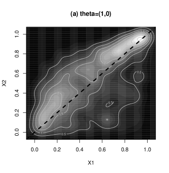
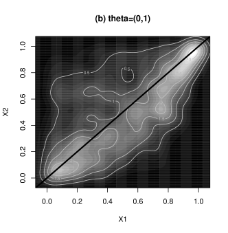
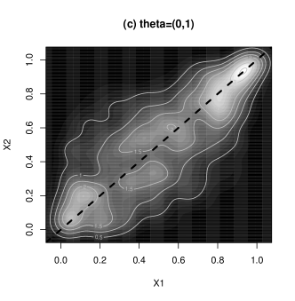
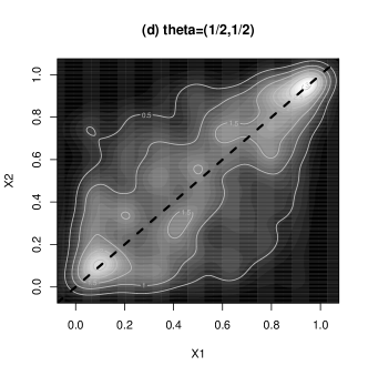
Figure 3: Image and contour plots of nonparametric density estimates for the simulated samples in figures 2a) through d).

Figures 2a) through d) show typical samples $\mathbf{X}_{i}=(X_{i1},X_{i2})\sim C(\cdot,\theta)$ ($i=1,2,...,n$) with $n=1000$, and $\mathbf{\theta}=(1,0)$, $(0,1)$, $(0,0)$ and $(\frac{1}{2},\frac{1}{2})$ respectively. Image (and contour) plots of two-dimensional kernel density estimates for these samples are shown in figures 3a) through 2d).

5.3 Simulation results

To study the finite sample performance of the estimators of $A$ discussed above, the following simulation study was carried out. For $\mathbf{\theta}=(0.1,0.1)$, $(0.05,0.9)$ and $(0.8,0.1)$ respectively, $1000$ simulated samples of size $n=25\cdot 2^{j}$ ($j=0,1,...,8$) were generated. For each sample, the nonparametric estimates $\widehat{A}$ and $\widehat{A}_{OLS}$ as well as the corresponding parametric estimates $A(\mathbf{w},\mathbf{\hat{\theta}}_{M})$ and $A(\mathbf{w},\mathbf{\hat{\theta}}_{M,OLS})$ were calculated. For $M$ (in $A(\mathbf{w},\mathbf{\hat{\theta}}_{M})$ and $A(\mathbf{w},\mathbf{\hat{\theta}}_{M,OLS})$), we used a discrete uniform distribution on the grid $\mathbf{w}_{i}=(w_{i1},1-w_{i2})$ ($w_{i1}=0.05\cdot i$, $i=1,2,...,19$). As expected, the naive nonparametric estimator $\hat{A}$ turned out to be clearly inferior to all other methods. For instance, for $\mathbf{\theta}=(0.1,0.1)$ and $n=50$, the integrated mean squared error $IMSE_{\text{nonp}}=\int_{\Delta_{2}}E[(\widehat{A}(\mathbf{w})-A(\mathbf{w}))^{2}]d\mathbf{w}$ is $74$ times larger than $IMSE_{\text{nonp},OLS}=\int_{\Delta_{2}}E[(\hat{A}_{OLS}(\mathbf{w})-A(\mathbf{w}))^{2}]d\mathbf{w}$, and $IMSE_{\text{par}}=\int_{\Delta_{2}}E[(A(\mathbf{w},\mathbf{\hat{\theta}}_{M})-A(\mathbf{w}))^{2}]d\mathbf{w}$ is almost $7$ times larger than the corresponding quantity (denoted by $IMSE_{\text{par},OLS}$) for $A(\mathbf{w},\mathbf{\hat{\theta}}_{M,OLS})$. For larger sample sizes the ratios

$$r_{\text{nonp}}=IMSE_{\text{nonp}}/IMSE_{\text{nonp},OLS}$$

and

$$r_{\text{par}}=IMSE_{\text{par}}/IMSE_{\text{par},OLS}$$

stabilize around the values of $64$ and $30$ respectively. Moreover, even if we compare the nonparametric OLS, $\hat{A}_{OLS}$, with the parametric estimator $A(\mathbf{w},\mathbf{\hat{\theta}}_{M})$, we obtain a ratio of $IMSE_{\text{par}}/IMSE_{\text{nonp},OLS}\approx 26$ for large sample sizes. We may thus conclude that using a good initial nonparametric estimator for the parametric method is essential. Detailed results on $\widehat{A}(\mathbf{w})$ and $A(\mathbf{w},\mathbf{\hat{\theta}}_{M})$ are therefore omitted, and we focus solely on the comparison between $\hat{A}_{OLS}$ and $A(\mathbf{w},\mathbf{\hat{\theta}}_{M,OLS})$. Figures 4a), b) and c) show the ratio $r=IMSE_{\text{par},OLS}/IMSE_{\text{nonp},OLS}$ for the three choices of $\mathbf{\theta}$ as a function of $n$. In all three cases, $r$ stabilizes around a value below $1$. The numerical values are given in table 1. As a function of $\mathbf{w}$, the relative precision of $\widehat{A}(\mathbf{w})$ compared to $A(\mathbf{w},\mathbf{\hat{\theta}}_{M,OLS})$ depends on $\mathbf{w}$ and the shape of $A$. This can be seen in figures 5a), b) and c), where simulated values of

$$r\left(\mathbf{w}\right)=\frac{E\left[\left(A(\mathbf{w},\mathbf{\hat{\theta}}_{M,OLS})-A(\mathbf{w})\right)^{2}\right]}{E\left[\left(\hat{A}_{OLS}(\mathbf{w})-A(\mathbf{w})\right)^{2}\right]}$$

are ploted as a function of $w_{1}$, for different values of $n$. Figures 6, 7 and 8, with estimates of $A$ for $50$ series of length $n=25$ (Fig. a,b) and $n=200$ (Fig. c,d) respectively, illustrate a further problem with the nonparametric OLS. For small sample sizes, $\hat{A}_{OLS}$ is often not exactly convex, which means that it is, with relatively high probability, not a proper dependence function. By definition, this problem does not occur for $A(\mathbf{w},\mathbf{\hat{\theta}}_{M,OLS})$. Finally, boxplots of $\hat{\theta}_{1}$ and $\hat{\theta}_{2}$ for the case with $\mathbf{\theta}=(0.05,0.9)$ are given in figures 9a) and b) respectively. One can see in particular that for small sample sizes the distributions of $\hat{\theta}_{1}$ and $\hat{\theta}_{2}$ are skewed to the right and left respectively. This is due to $\theta_{1}$ and $\theta_{2}$ being close to the border of the parameter space, and the restrictions $\theta_{1},\theta_{2}\geq 0$ and $\theta_{1}+\theta_{2}\leq 1$.

6 Final remarks

In this paper we considered estimation of extreme value copulas based on parametric models that are defined in terms of the spectral measure. This approach is very flexible, and in principle any type of dependence between extremes can be captured. The method is not restricted to the case where the marginal distributions are known, since any nonparametric estimator $\hat{A}$ can be used in the projection. Theorem 1 and Corollary 1 apply (with $\sigma\left(\mathbf{v},\mathbf{w}\right)$ replaced by the corresponding asymptotic covariance function) whenever a functional limit theorem of the form given in (8) holds for $\hat{A}$.

An important issue that would need to be addressed in future research is the extension to a larger class of copulas. In this paper, observations were assumed to be generated by an extreme value copula. In practice, an extreme value copula is usually reached only asymptotically (for multivariate maxima). In analogy to nonparametric extreme value copula estimators, consistent parametric methods will have to be developed for such situations. A further question is model choice, i.e. the question how to decide on the number and type of spectral measures to be used as a basis. For data generated by an extreme value copula, standard methods such as AIC or BIC ([1],[16]) may be useful. In the more general situation where an extreme value copula is only reached in the limit, the question is more complex.

7 Acknowledgements

This research has been supported in part by the DFG-Research Grant BE 2123/11-1. Georg Mainik would like to thank RiskLab, ETH Zurich, for financial support.

$n$	$\mathbf{\theta}=(0.1,0.1)$	$\mathbf{\theta}=(0.05,0.9)$	$\mathbf{\theta}=(0.8,0.1)$
$25$	0.375	0.504	0.480
$50$	0.444	0.622	0.652
$100$	0.512	0.636	0.696
$200$	0.613	0.652	0.767
$400$	0.756	0.674	0.815
$800$	0.840	0.749	0.876
$1600$	0.899	0.805	0.898
$3200$	0.903	0.868	0.900
$6400$	0.902	0.887	0.903

Table 1: $r=IMSE_{{\rm par},OLS}/IMSE_{{\rm nonp},OLS}$ for $\mathbf{\theta}=(0.1,0.1)$, $(0.05,0.9)$ and $\mathbf{\theta}=(0.8,0.1)$ respectively, and sample sizes $n=25\cdot 2^{j}$ $(j=0,1,...,8)$.

Figure 2: Simulated samples $\mathbf{X}_{i}=(X_{i1},X_{i2})\sim C(\cdot,\theta)$ ($i=1,2,...,n$) with $n=1000$, and $\mathbf{\theta}=(1,0)$, $(0,1)$, $(0,0)$ and $(\frac{1}{2},\frac{1}{2})$ respectively.

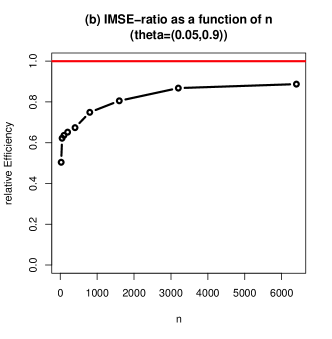
Figure 4: Ratio of parametric and nonparametric IMSE for (a) $\mathbf{\theta}=(0.1,0.1)$, (b) $(0.05,0.9)$ and (c) $(0.8,0.1)$ respectively.

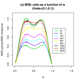
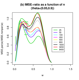
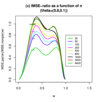
Figure 5: Ratio of parametric and nonparametric MSE, $r\left(\mathbf{w}\right)$, for (a) $\mathbf{\theta}=(0.1,0.1)$, (b) $(0.05,0.9)$ and (c) $(0.8,0.1)$, and sample sizes $n=$25, 50, 100, 200, 400, 800, 1600, 3200 and 6400 respectively.

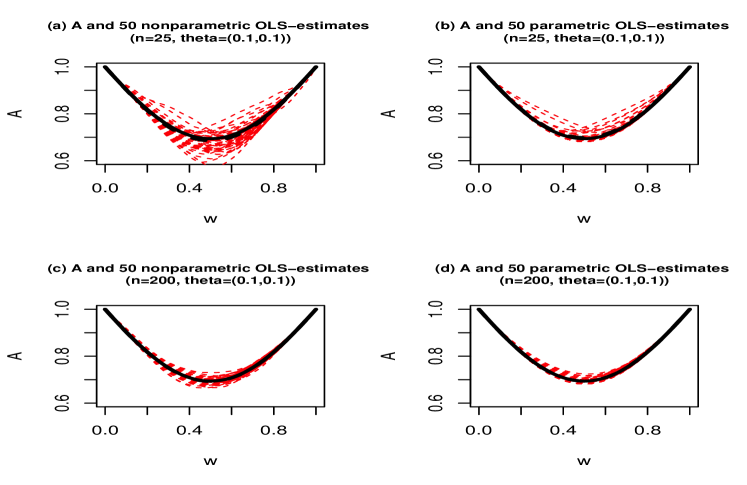
Figure 6: 50 estimates $\hat{A}_{OLS}(\mathbf{w})$ (fig. (a) and (c)) and $A\left(\mathbf{w},\mathbf{\hat{\theta}}_{M,OLS}\right)$ for $\theta=(0.1,0.1)$ and $n\in\{25,\ 200\}$. The black line represents the true function $A$.

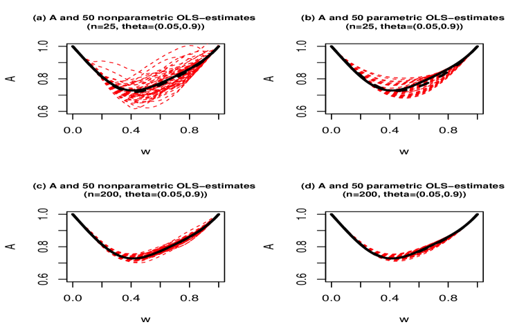
Figure 7: 50 estimates $\hat{A}_{OLS}(\mathbf{w})$ (fig. (a) and (c)) and $A(\mathbf{w},\mathbf{\hat{\theta}}_{M,OLS})$ for $\theta=(0.05,0.9)$ and $n\in\{25,\ 200\}$. The black line represents the true function $A$.

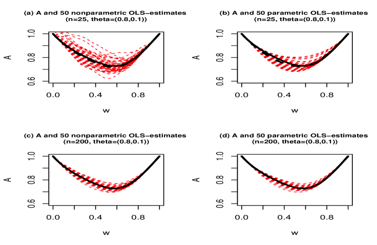
Figure 8: 50 estimates $\hat{A}_{OLS}(\mathbf{w})$ (fig. (a) and (c)) and $A(\mathbf{w},\mathbf{\hat{\theta}}_{M,OLS})$ for $\theta=(0.8,0.1)$ and $n\in\{25,\ 200\}$. The black line represents the true function $A$.

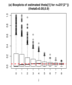
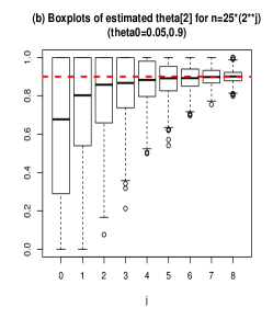
Figure 9: Boxplots of $\hat{\theta}_{OLS,1}$ (fig. a) and $\hat{\theta}_{OLS,2}$ (fig. b) for the case with $\mathbf{\theta}=(0.05,0.9)$, and $n=25\cdot 2^{j}$ $(j=0,1,...,8)$. The horizontal line represents the true value of $\theta_{i}$ ($i=1,2$).

References

- [1] Akaike, H. (1973). Information theory and an extension of the maximum likelihood principle. In: B. N. Petrov (Ed.), Proceedings of the Second International Symposium on Information Theory. Budapest: Akademiai Kiado, pp. 267-281.
- [2] Boldi, M.-O. and Davison, A. C. (2007). A mixture model for multivariate extremes. Journal of the Royal Statistical Society, Series B, Vol. 69, No. 2, 217–229.
- [3] Capéraà, P., Fougères, A.-L. and Genest, C. (1997). A nonparametric estimation procedure for bivariate extreme value copulas. Biometrika, Vol. 84, No. 3, 567–577.
- [4] de Haan, L. and Resnick, S.I. (1977). Limit theory for multivariate sample extremes. Z. Wahrscheinlichkeitstheorie und Verw. Gebiete, Vol. 40, No. 4, 317–337.
- [5] Deheuvels, P. (1991). On the limiting behavior of the Pickands estimator for bivariate extreme-value distributions. Statist. Probab. Lett., Vol. 12, No. 5, 429–439.
- [6] Fils-Villetard, A., Guillou, A. and Segers, J. (2008). Projection estimators of Pickands dependence functions. Canad. J. Statist., Vol. 36, No. 3, 369–382.
- [7] Genest, C. and Rivest, L.-P. (1989). A characterization of Gumbel’s family of extreme value distributions. Stat. Probab. Lett., Vol. 8, No. 3, 207–211.
- [8] Ghoudi, K., Khoudraji, A. and Rivest, L.-P. (1998). Propriétés statistiques des copules de valeurs extrêmes bidimensionelles. Canad. J. Statist., 26, 187-197.
- [9] Gudendorf, G. and Segers, J. (2010). Extreme-Value Copulas. In: Copula Theory and Its Applications, Bickel, P., Diggle, P., Fienberg, S., Gather, U., Olkin, I., Zeger, S., Jaworski, P., Durante, F., Härdle, W.K. and Rychlik, T. (eds.), Lecture Notes in Statistics, Vol. 198, Springer Berlin/Heidelberg, pp. 127-145.
- [10] Gudendorf, G. and Segers, J. (2011). Nonparametric estimation of an extreme-value copula in arbitrary dimensions. J. Multiv. Anal., Vol. 102, No. 1, 37 - 47.
- [11] Gudendorf, G. and Segers, J. (2012). Nonparametric estimation of multivariate extreme-value copulas. J. Statist. Plann. Inference, Vol. 142, No. 12, 3073–3085.
- [12] Guillotte, S. Perron, F. and Segers, J. (2011). Non-parametric Bayesian inference on bivariate extremes. Journal of the Royal Statistical Society, Series B, Vol. 73, No. 3, 377–406.
- [13] Hall, P. and Tajvidi, N. (2000). Distribution and dependence-function estimation for bivariate extreme-value distributions. Bernoulli, Vol. 6, No. 5, 835–844.
- [14] Mai, J.-F. and Scherer, M. (2011). Bivariate extreme-value copulas with discrete Pickands dependence measure. Extremes, Vol. 14, No. 3, 311-324.
- [15] Pickands, J. (1981). Multivariate extreme value distributions. Bulletin de l’Institut International de Statistique, Vol. 49, 859–878 and 894–902.
- [16] Schwarz, G. (1978). Estimating the dimension of a model. Annals of Statistics, Vol. 2, No. 6, 461-464.
- [17] Zhang, D., Wells, M.T. and Peng, L.. (2008). Nonparametric estimation of the dependence function for a multivariate extreme value distribution. J. Multiv. Anal., Vol. 99, No. 4, 577–588.