Constraining $f(R)$ theories with cosmography

Abstract

A method to set constraints on the parameters of extended theories of gravitation is presented. It is based on the comparison of two series expansions of any observable that depends on $H(z)$. The first expansion is of the cosmographical type, while the second uses the dependence of $H$ with $z$ furnished by a given type of extended theory. When applied to $f(R)$ theories together with the redshift drift, the method yields limits on the parameters of two examples (the theory of Hu and Sawicki Hu and Sawicki (2007), and the exponential gravity introduced by Linder Linder (2009)) that are compatible with or more stringent than the existing ones, as well as a limit for a previously unconstrained parameter.

I Introduction

The interpretation of several sets of data (such as those obtained from type Ia supernovae, large scale structure, baryon acoustic oscillations, and the cosmic microwave background) in the framework of the Standard Cosmological Model (SCM) (based on General Relativity (GR) and the Cosmological Principle) indicates that the universe is currently undergoing a phase of accelerated expansion. The most commonly accepted candidates to source such an expansion (namely, the cosmological constant, and some unknown type of matter dubbed “dark energy” ) are not free of problems. While the energy density associated with the cosmological constant that is inferred from astronomical observations is approximately 120 orders of magnitude lower than the value predicted by field theory (see for instance Capozziello and Faraoni (2011)), the scalar field used to model dark energy has features that are alien to those displayed by the scalar fields of particle physics Sotiriou and Faraoni (2010). An alternative way to describe the accelerated expansion is to assume that it is produced by the dynamics of a theory which differs from GR after matter domination. Among these, the so-called $f(R)$ theories, with action given by

$$S=\int\sqrt{-g}f(R){\rm d}^{4}x,$$

are the simplest generalization of the Einstein-Hilbert Lagrangian. The dependence of the function $f$ on the scalar curvature $R$ is to be determined by several criteria (such as matter stability Dolgov and Kawasaki (2003), absence of ghost modes in the cosmological perturbations Carroll et al. (2003), correct succession of cosmological eras Amendola et al. (2007), and the stability of cosmological perturbations Bean et al. (2007)) . Several forms for $f(R)$ have been constructed in order to successfully satisfy these constraints (for instance those given in (Starobinsky, 2007; Hu and Sawicki, 2007)), allowing in principle (potentially small) deviations from GR, quantified by some of the parameters of the $f(R)$. We shall introduce here a method that can be used to set limits on the parameters of a given $f(R)$, which is based in the comparison of two series expansions in terms of the redshift $z$. The first one is that of any observable quantity given in terms of $H(z)$ , and the second, the corresponding cosmographic expansion. While the former depends on the dynamics of the theory, the latter does not (see Sect. II). The order-by-order comparison of these expansions yields relations among $f$, its derivatives w.r.t. $R$, and the kinematical parameters (some of which are determined by observation), all at $t=\$ today. By rewritting these relations in terms of the parameters of a given $f$, the abovementioned limits can be obtained.

It is important to emphasize that the method does not rely on the actual measurement of the observable: it only demands that the expression of the observable obtained using the dynamics coincides with that obtained in a dynamic-independent way (namely, using cosmography). Although it can be applied to any observable expressed in terms of $H(z)$, yielding for each observable different limits on the parameters of the $f(R)$, the method is more useful in the case of yet-to-be measured quantities, of which only the cosmographical form has been determined.

Currently a lot of effort is devoted to the study of quantities and effects that have the potential of discriminating between different $f(R)$ models, and between these models and GR. Among them, we can mention the growth rate of matter density perturbations (see for instance Carroll et al. (2006)), the enhanced brightness of dwarf galaxies Davis et al. (2012), the modifications of the 21cm power spectrum at reionisation Brax et al. (2013), the specific angular momentum of galactic halos Lee et al. (2013), and the number counts of peaks in weak lensing maps Cardone et al. (2012). We shall apply our method to the Redshift Drift (RD), that is, the time variation of the cosmological redshift caused by the expansion of the Universe. The RD was first considered by Sandage (1962), and the effects of a nonzero cosmological constant on it were presented in McVittie (1962). As discussed in Quercellini et al. (2012), its measurement is feasible in the near future. As soon as data related to the RD become available, they could be compared with the prediction of a given $f(R)$, adjusting the parameters of the theory to describe the data. We propose here the alternative route presented above, namely the comparison of the “cosmographical RD” with the “dynamical RD”, the results of which must be compatible with those that will come from the actual measurements.

When compared to other cosmological observables, the RD has the advantage that it directly tests the dependence of the Hubble parameter with the redshift, hence probing the dynamics of the scale factor. Another feature of this observable is that it does not depend on details of the source (such as the absolute luminosity), or on the definition of a standard ruler. As demonstrated in Uzan et al. (2008), the RD would allow the test of the Copernican Principle, thus checking for any degree of radial inhomogeneity. This issue was further discussed in (Quartin and Amendola, 2010), where it was shown that the RD is positive for sources with $z<2$ in the $\Lambda$CDM, while in Lemâitre-Tolman-Bondi models is negative for sources observed from the symmetry center (Yoo et al., 2011). The RD can also be used to constrain phenomenological parametrizations of dynamical dark energy models (see Vielzeuf and Martins (2012); Martinelli et al. (2012a); Moraes and Polarski (2011)). To use the RD as an example of our method, we shall work out in Sect. II the series expansion of this observable in terms of the cosmological redshift $z$ and the time derivatives of the scale factor (i.e. the kinematical parameters). Since the RD depends on the explicit form of the Hubble parameter $H(z)$, we shall show in Sect. III that its series expansion in $z$ can be written in terms of $f(R)$ and its derivatives, using the equations of motion (EoM) of a yet unspecified $f(R)$ theory in the metric version. By comparing the two series, it will be shown that there exists relations between $f(R)$, its derivatives, and the kinematical parameters, which impose constraints on the parameters of a given $f(R)$. These constraints will be analyzed on two examples: that proposed by Hu and Sawicki (2007) (see Sect.III.1), and the exponential gravity theory introduced by Linder (2009)(see Sect.III.2). In both cases, we find limits on the parameters of these $f(R)$ theories that are compatible with or more stringent than the existing ones, as well as a limit for a previously unconstrained parameter. We close in Sect. IV with some remarks.

II A cosmographical approach to the redshift drift

Cosmography is a mathematical framework for the description of the universe, based entirely on the Cosmological Principle, and on those parts of GR that follow directly from the Principle of Equivalence (Weinberg, 1972). It is inherently kinematic, in the sense that it is independent of the dynamics obeyed by the scale factor $a(t)$. In this section we shall present the calculation, in the context of cosmography, that leads to the series expansion of the RD in terms of $z$, assuming only that spacetime is homogeneous and isotropic.

The redshift of a photon emitted by a source at time $t$ that reaches the observer at time $t_{obs}$ is given by

$$z(t)=\frac{a(t_{obs})}{a(t)}-1.$$ (1)

The time variation of the redshift is obtained by comparing this expression with the one corresponding to a photon emitted at $t^{\prime}=t+\Delta t$, that is $\Delta z=z(t+\Delta t)-z(t)$. To first order in $\Delta t_{obs}$ and $\Delta t$, it follows that (Loeb, 1998)

$$\frac{\Delta z}{\Delta t_{obs}}=\left[\frac{\dot{a}(t_{obs})-\dot{a}(t)}{a(t)}\right].$$ (2)

Using the definition of $z$ and $H(z)$ in this equation we get the expression of the RD in terms of $z$, namely

$$\frac{\Delta z}{\Delta t_{obs}}=(1+z)H_{obs}-H(z).$$ (3)

Next, an expansion of $H$ in powers of $z$ will be obtained, using the cosmographical approach, while in the next section we will exhibit the analogous expansion using the form of $H$ determined by a given $f(R)$ theory. The series development of the scale factor around $t_{0}=t_{obs}$ is given by

$$a(t)=a_{0}\left[1+H_{0}(t-t_{0})-\frac{1}{2}q_{0}H_{0}^{2}(t-t_{0})^{2}+\frac{1}{3!}j_{0}H_{0}^{3}(t-t_{0})^{3}+\frac{1}{4!}s_{0}H_{0}^{4}(t-t_{0})^{4}+{\cal O}([t-t_{0}]^{5})\right],$$ (4)

where the so-called kinematical parameters are defined by

$$H(t)\equiv+\frac{1}{a(t)}\frac{{\rm d}a}{{\rm d}t},\ \ q(t)\equiv-\frac{1}{a(t)}\frac{{\rm d}^{2}a}{{\rm d}t^{2}}\left[\frac{1}{a(t)}\frac{{\rm d}a}{{\rm d}t}\right]^{-2},\ \ j(t)\equiv+\frac{1}{a(t)}\frac{{\rm d}^{3}a}{{\rm d}t^{3}}\left[\frac{1}{a(t)}\frac{{\rm d}a}{{\rm d}t}\right]^{-3},\ s(t)\equiv+\frac{1}{a(t)}\frac{{\rm d}^{4}a}{{\rm d}t^{4}}\left[\frac{1}{a(t)}\frac{{\rm d}a}{{\rm d}t}\right]^{-4}.$$

In order to use Eq. (4) for the calculation of the RD, we need to express $t$ in terms of known quantities. This can be achieved through the physical distance travelled by a photon emitted at $t$ and observed at $t_{0}$, given by

$$D=c\int{\rm d}t=c(t_{0}-t).$$ (5)

A relation between $D$ and $z$ can be obtained from Eq. (1) Visser (2005):

$$1+z=\frac{a(t_{0})}{a(t)}=\frac{a(t_{0})}{a(t_{0}-D/c)}.$$ (6)

Performing a Taylor series expansion, Eq. (6) yields

$$z(D)=\frac{H_{0}D}{c}+\frac{2+q_{0}}{2}\frac{H_{0}^{2}D^{2}}{c^{2}}+\frac{6(1+q_{0})+j_{0}}{6}\frac{H_{0}^{3}D^{3}}{c^{3}}+{\cal O}\left(\left[\frac{H_{0}D}{c}\right]^{4}\right),$$ (7)

which can be inverted to

$$D(z)=\frac{c\ z}{H_{0}}\left[1-\left(1+\frac{q_{0}}{2}\right)z+\left(1+q_{0}+\frac{q_{0}^{2}}{2}-\frac{j_{0}}{6}\right)z^{2}-\left(1+\frac{3}{2}q_{0}(1+q_{0})+\frac{5}{8}q_{0}^{3}-\frac{1}{2}j_{0}-\frac{5}{12}q_{0}j_{0}-\frac{s_{0}}{24}\right)z^{3}+{\cal O}(z^{4})\right].$$ (8)

Setting $t=t_{0}-D/c$, the Taylor expansion of expression (2) yields

$$\frac{\Delta z}{\Delta t_{0}}(D)=-q_{0}H_{0}^{2}\frac{D}{c}-\frac{1}{2}H_{0}^{3}(j_{0}+2q_{0})\left(\frac{D}{c}\right)^{2}-\frac{1}{6}H_{0}^{4}[3q_{0}(q_{0}+2)-s_{0}+3j_{0}]\left(\frac{D}{c}\right)^{3}+{\cal O}(D^{4}).$$ (9)

Lastly, using Eq. (8) we can write the RD as a power series in $z$, with coefficients that are functions of the kinematical parameters in the form

$$\frac{\Delta z}{\Delta t_{0}}(z)=-H_{0}q_{0}z+\frac{1}{2}H_{0}\left(q_{0}^{2}-j_{0}\right)z^{2}+\frac{1}{2}H_{0}\left[\frac{1}{3}\left(s_{0}+4q_{0}j_{0}\right)+j_{0}-q_{0}^{2}-q_{0}^{3}\right]z^{3}+{\cal O}(z^{4}).$$ (10)

This equation gives the cosmographical expression of the RD up to the third order in the redshift of the source, in terms of the value of the kinematical parameters at the present epoch (whose values are known from observation, see Sect.III.1). Let us remark that Eq. (10) is completely independent of the dynamics obeyed by the gravitational field. Hence, any viable theory must yield a prediction for the RD compatible with it. In the next section, this expression will be compared with that obtained using the dynamics of an arbitrary $f(R)$ theory.

III The Redshift Drift in $f(R)$ Theories

Let us recall that the RD can be expressed in terms of $H(z)$ as follows

$$\frac{\Delta z}{\Delta t_{0}}=(1+z)H_{0}-H(z).$$ (11)

In the case of the SCM, the RD can be written as a function of the cosmological parameters $H_{0}$, $\Omega_{m,0}$, $\Omega_{r,0}$ and $\Omega_{\Lambda,0}$ using the exact expression for $H(z)$ as follows (Loeb, 1998):

$$\frac{\Delta z}{\Delta t_{0}}=H_{0}\left[(1+z)-\left(\Omega_{m,0}(1+z)^{3}+\Omega_{r,0}(1+z)^{4}+\Omega_{\Lambda,0}\right)^{1/2}\right],$$ (12)

where the subindex 0 means that the corresponding quantity is evaluated at $t=$ today. In the case of $f(R)$ theories, the expression for $H$ that follows from the variation of the action

$$S=\int{\rm d}^{4}x\sqrt{-g}\left[{f(R)}+{\cal L}_{\rm matter}\right]$$

w.r.t. the metric must be used. For the FLRW metric and considering a pressureless cosmological fluid, these equations are (see for instance Kerner (1982))

$$f^{\prime}R-2f-3f^{\prime\prime}\left(\ddot{R}+\frac{3\dot{a}\dot{R}}{a}\right)-3f^{\prime\prime\prime}\dot{R}^{2}=T,$$ (13)

$$f^{\prime}R_{tt}+\frac{1}{2}f+3f^{\prime\prime}\frac{\dot{a}\dot{R}}{a}=T_{tt},$$ (14)

where dot and prime denote, respectively, derivative w.r.t. $t$ and $R$, $R_{tt}=3\ddot{a}/a$, $R=6(\frac{\ddot{a}}{a}+\frac{\dot{a}^{2}}{a^{2}})$, and $T$ is the trace of the energy-momentum tensor. From these, the following relation can be obtained (Capozziello et al., 2008):

$$H=\frac{1}{6\dot{R}f^{\prime\prime}}\left(6H^{2}f^{\prime}-2\rho_{m}-f+Rf^{\prime}\right),$$ (15)

with $\rho_{m}=\rho_{m,0}a^{-3}=3H_{0}^{2}\Omega_{m,0}a^{-3}$. Using this expression in Eq. (11) we find

$$\frac{\Delta z}{\Delta t_{0}}(z)=\frac{\dot{a}_{0}-\dot{a}(z)}{a(z)}=H_{0}\left\{(z+1)-\frac{1}{6}\frac{f(R)-Rf^{\prime}(R)+6H^{2}f^{\prime}(R)-2\rho_{m}}{H_{0}\dot{R}(t)f^{\prime\prime}(R)}\right\},$$ (16)

where $f$, $R$, $H$, and $\rho_{m}$ are functions of $z$ . We use $\frac{{\rm d}f}{{\rm d}z}=\frac{{\rm d}f}{{\rm d}R}\frac{{\rm d}R}{{\rm d}t}\frac{{\rm d}t}{{\rm d}z}$ and analogous expressions for other quantities to expand Eq. (16) in powers of $z$. To first order, the result for an arbitrary $f(R)$ is given by

$$\frac{\Delta z}{\Delta t_{0}}(z) = \left\{H_{0}+\frac{1}{6H_{0}f^{\prime\prime}_{0}}\left[\frac{1}{\dot{R}_{0}}\left(f^{\prime\prime}_{0}\dot{R}_{0}(R_{0}-6H_{0}^{2})+2\dot{\rho}_{m,0}-12H_{0}\dot{H}_{0}f^{\prime}_{0}\right)\right.\right.\qquad\qquad\qquad\qquad\qquad\qquad\qquad$$ (17)

$$\qquad\qquad\qquad\qquad\qquad\qquad\qquad\left.\left.+\left(\frac{\ddot{R}_{0}}{\dot{R}^{2}_{0}}+\frac{f^{\prime\prime\prime}_{0}}{f^{\prime\prime}_{0}}\right)\left(f_{0}+f^{\prime}_{0}(6H_{0}^{2}-R_{0})-2\rho_{m,0}\right)\right]\right\}z+{\cal O}(z^{2}).\$$

Lastly, using that $R_{0}=6(\dot{H}_{0}+2H_{0}^{2})$, $\dot{H}_{0}=-H_{0}^{2}(1+q_{0})$ and $\ddot{H}_{0}=H_{0}^{3}(j_{0}+3q_{0}+2)$ together with the definitions of the kinematical parameters, we obtain

$$\frac{\Delta z}{\Delta t_{0}}(z) = \left\{\left[6q_{0}H_{0}^{2}f^{\prime}_{0}+f_{0}-6\Omega_{m,0}H_{0}^{2}\right](j_{0}-q_{0}-2)^{2}\frac{f^{\prime\prime\prime}_{0}}{6f^{\prime\prime}_{0}}+\right.$$ (18)

$$\quad+H_{0}^{2}f^{\prime\prime}_{0}\left[(j_{0}-2)^{2}-q_{0}(3q_{0}+(q_{0}-j_{0})^{2}-2j_{0})\right]+f^{\prime}_{0}[q_{0}(q_{0}^{2}+6q_{0}+2j_{0}+s_{0})+2j_{0}+4]$$

$$\left.\qquad\quad+\frac{f_{0}}{36H_{0}^{2}}(-s_{0}-q_{0}^{2}-6-8q_{0})+\frac{\Omega_{m,0}}{6}(s_{0}+3j_{0}+5q_{0}+q_{0}^{2})\right\}\frac{z}{f^{\prime\prime}_{0}H_{0}(j_{0}-q_{0}-2)^{2}}+{\cal O}(z^{2}).\$$

The dependence of the RD with the given theory is manifest in Eq. (18) through $f$ and its derivatives evaluated today. We can now compare the linear term in $z$ of the kinematical and dynamic approaches to the RD, given by Eqs. (10) and (18), respectively. The result is a relation between $f(R)$, its derivatives and the kinematical parameters, all evaluated at $t=$ today:

$$\left\{[q_{0}(q_{0}(q_{0}+6)+2j_{0}+s_{0})+2(j_{0}-2)]f^{\prime}_{0}+[s_{0}+q_{0}(q_{0}+8)+6]f_{0}-[q_{0}(q_{0}+5)+s_{0}+3j_{0}]\Omega_{m,0}\right\}f^{\prime\prime}_{0}+$$

$$\left[(q_{0}-j_{0})^{2}+4(1+q_{0}-j_{0})\right]\left\{f_{0}f^{\prime\prime\prime}_{0}+6H_{0}^{2}[(q_{0}f^{\prime}_{0}-\Omega_{m,0})f^{\prime\prime\prime}_{0}+(f^{\prime\prime}_{0})^{2}]\right\} = 0.\ \qquad$$ (19)

Notice that the restriction to the first order in $z$ is not related to actual measurements of the RD for sources with $z\ll 1$, but to the fact that the second order term depends on ${\ell}_{0}$, for which there are no observational limits available. Note also that Eq. (III) is a necessary condition for any $f(R)$ theory to describe the variation of the RD with $z$. By equating higher orders of $z$ from Eqs. (10) and (18) we would obtain more (actually, an infinite number of) necessary conditions on $f(R)$ and its derivatives. If the theory under discussion is to describe the RD at all orders in $z$, all these conditions should be satisfied.

We shall see next how Eq. (III) constrains the value of the parameters of a given $f(R)$, by applying it to two examples.

III.1 Example 1: The Theory of Hu and Sawicki

Let us start with the theory introduced by Hu and Sawicki (2007), which is given by

$$f(R)=R-m^{2}\frac{c_{1}(R/m^{2})^{n}}{c_{2}(R/m^{2})^{n}+1},$$ (20)

where $n>0$, $c_{1}$ and $c_{2}$ are dimensionless parameters and the mass scale is $m^{2}\equiv\kappa^{2}\bar{\rho}_{0}/3$, with $\bar{\rho}_{0}$ the average density today.

For values of the curvature high compared with $m^{2}$ (which is actually the case if the current accelerated expansion is to be not very different today from that in GR+$\Lambda$, see Hu and Sawicki (2007)), $f(R)$ may be expanded as

$$\lim_{m^{2}/R\rightarrow 0}f(R)\simeq R-\frac{c_{1}}{c_{2}}m^{2}+\frac{c_{1}}{c_{2}^{2}}m^{2}\left(\frac{m^{2}}{R}\right)^{n}$$ (21)

and, at finite $c_{1}/c_{2}^{2}$, the theory can approximate the expansion history of the $\Lambda$CDM model (Hu and Sawicki, 2007). In this regime, the parameters $c_{1}$ and $c_{2}$ must satisfy the relation

$$\frac{c_{1}}{c_{2}}\approx 6\frac{\tilde{\Omega}_{\Lambda}}{\tilde{\Omega}_{m}}.$$ (22)

For the flat $\Lambda$CDM expansion history, Eq. (21) yields

$$R \simeq 3m^{2}\left(a^{-3}+4\frac{{\tilde{\Omega}}_{\Lambda}}{{\tilde{\Omega}}_{m}}\right),$$ (23)

$$f^{\prime} \simeq 1-n\frac{c_{1}}{c_{2}^{2}}\left(\frac{m^{2}}{R}\right)^{n+1},$$ (24)

and at the present epoch,

$$R_{0} \simeq m^{2}\left(\frac{12}{{\tilde{\Omega}}_{m,0}}-9\right),$$ (25)

$$f^{\prime}_{0} \simeq 1-n\frac{c_{1}}{c_{2}^{2}}\left(\frac{12}{{\tilde{\Omega}}_{m,0}}-9\right)^{-n-1}.$$ (26)

Using Eq. (26), $c_{1}/c_{2}^{2}$ can be expressed in terms of $n$, $f^{\prime}_{0}$ and ${\tilde{\Omega}}_{m,0}$. In addition, higher order derivatives of $f$ can also be written in terms of the same quantities. Hence from now on we set ${\tilde{\Omega}}_{m,0}=0.274\pm 0.007$ (Komatsu et al., 2011) and leave $f^{\prime}_{0}$ and $n$ the only free parameters of the theory. With these considerations, Eq. (III) yields

$$f^{\prime}_{0}(n) = \frac{1}{A}\left\{[q_{0}(5q_{0}-6j_{0}+8+(q_{0}-j_{0})^{2})+(j_{0}-2)^{2}]4n+[j_{0}(j_{0}-8)-2q_{0}(j_{0}+q_{0}+8)-3(s_{0}+2)]6{\tilde{\Omega}}_{m,0}\right.\qquad\quad$$ (27)

$$\left.\qquad\qquad\quad\ +[2(j_{0}+1)+q_{0}(q_{0}+6)+s_{0}]9{\tilde{\Omega}}_{m,0}^{2}+[q_{0}(2(10+3q_{0}-2j_{0})+(q_{0}-j_{0})^{2})+2(s_{0}+6)]4\right\},\$$

with

$$A = [q_{0}((q_{0}-j_{0})^{2}-6j_{0}+8+5q_{0})+(j_{0}-2)^{2}]4n-[3s_{0}+18+22q_{0}-(j_{0}-2)^{2}+(2q_{0}+1)^{2})]6{\tilde{\Omega}}_{m,0}\qquad\qquad\quad$$ (28)

$$\qquad\qquad\qquad\qquad+[s_{0}+q_{0}^{2}+8q_{0}+6]9{\tilde{\Omega}}_{m,0}^{2}+[q_{0}(2(5q_{0}+16-4j_{0})+(q_{0}-j_{0})^{2})+2(s_{0}+10-2j_{0})]4.$$

Expression (27) gives a relation between the parameters $f^{\prime}_{0}$ and $n$ in terms of ${\tilde{\Omega}}_{m}$ and the kinematical parameters $H$, $q$, $j$, and $s$, all evaluated today. We shall take the values $q_{0}=-0.669\pm 0.052$, $j_{0}=0.284\pm 0.151$ and $s_{0}=-0.680\pm 0.456$ (Capozziello et al., 2011). In Figure 1 we plot the relation $f^{\prime}_{0}(n)$ provided by our cosmographical approach to the RD combined with the expansion of the expression of $H(z)$ for $f(R)$ theories . The curve tends asymptotically to $f^{\prime}_{0}=1$, which corresponds to the GR limit. The plot also displays the limit obtained from solar system tests, given by $|f^{\prime}_{0}-1|<0.1$ (Hu and Sawicki, 2007). We find that actually $1-f^{\prime}_{0}<0.1$ and, from this limit, values for $n$ larger than approximately $3$ are favoured, thus discarding low values for $n$, and allowing for large values, in accordance with the findings of (Martinelli et al., 2012b).

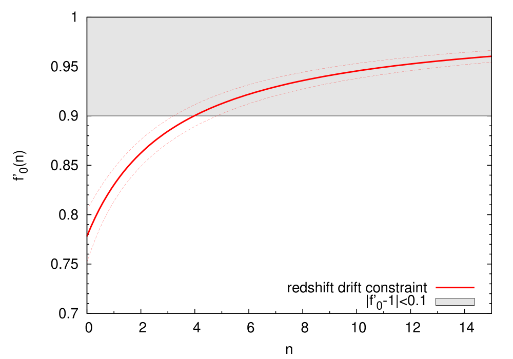
Figure 1: Constraints on the parameter space of the theory by Hu and Sawicki. The red line corresponds to the relation between $f^{\prime}_{0}$ and $n$ that follows from Eq. (III). The dashed lines represent the error propagation arising from the kinematical parameters and the density matter at the present epoch. The shady region indicates the values of $f^{\prime}_{0}$ in agreement with solar system tests.

III.2 Example 2: Exponential Gravity

Next we shall analyze the restrictions that follow from Eq. (III) on the choice of $f(R)$ proposed by Linder (2009):

$$f(R)=R-cr(1-\exp(-R/r)),$$ (29)

where $c$ and $r$ are two (positive) parameters of the model. This $f(R)$ was specifically designed to (i) avoid the inclusion of an implicit cosmological constant (since it vanishes in the low curvature limit), (ii) reduce to GR for high values of the curvature, (iii) incorporate a transition scale (given by $r$) to be fitted from observations (instead of set equal to $R_{0}$), and (iv) restore GR for locally high curvature systems such as the solar system or galaxies. As shown in (Linder, 2009), the product $cr$ is given in terms of $\Omega_{m,0}$ by

$$cr=6m^{2}(\Omega_{m,0}^{-1}-1).$$ (30)

The use of Eq. (III) for the current choice of $f(R)$ yields a relation between the dimensionless parameters $c$ and $r/m^{2}$ given by

$$c\left(\frac{r}{m^{2}}\right) = \frac{1}{B}\left\{\left[(3+s_{0}+2j_{0}(q_{0}+1)-(q_{0}-1)^{2})-(q_{0}(q_{0}+5)+s_{0}+q_{0}^{2}+3j_{0})\Omega_{m,0}\right]6\Omega_{m,0}\frac{r}{m^{2}}\right.\qquad\qquad\qquad\qquad$$ (31)

$$\qquad\qquad\qquad\qquad\qquad\qquad\qquad\qquad\left.+[4(1+q_{0}-j_{0})+(q_{0}-j_{0})^{2}]36\left(\Omega_{m,0}-1\right)\right\}\exp\left(\frac{6(1-q_{0})}{\frac{r}{m^{2}}\Omega_{m,0}}\right),\ \ \$$

with

$$B = \left\{[q_{0}(q_{0}+8)+6+s_{0}]\Omega_{m,0}\left(\frac{r}{m^{2}}\right)\left[(\exp\left(\frac{6(1-q_{0})}{\frac{r}{m^{2}}\Omega_{m,0}}\right)-1\right]-6[4(1+q_{0}-j_{0})+(q_{0}-j_{0})^{2}]\exp\left(\frac{6(1-q_{0})}{\frac{r}{m^{2}}\Omega_{m,0}}\right)\right.$$ (32)

$$\left.+6[q_{0}(q_{0}(q_{0}+7)+4+s_{0})+(j_{0}-1)^{2}-1]\right\}\Omega_{m,0}\left(\frac{r}{m^{2}}\right)-[(j_{0}-2)^{2}+q_{0}((q_{0}-j_{0})^{2}+8-6j_{0}+5q_{0})]36,$$

which is plotted along with Eq. (30) in Figure 2 . The strips formed by both curves and the corresponding errors juxtapose for all values of $c\gtrsim 6$, which imply that $r/m^{2}\lesssim 2.7$.

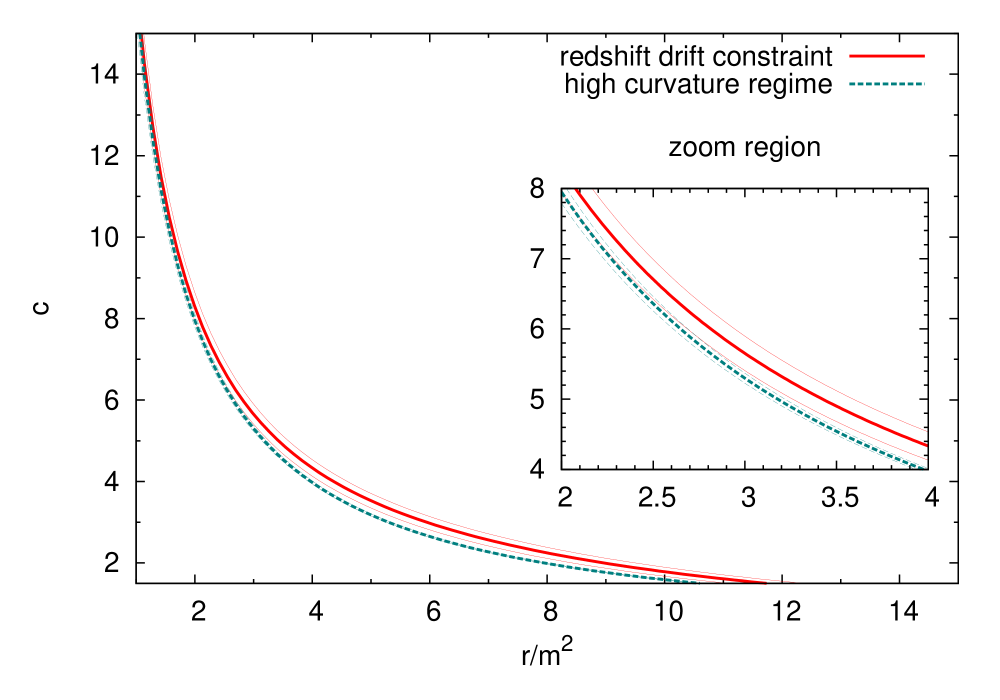
Figure 2: Constraints coming from our approach to the redshift drift (continuous line) and the relation (30) between the parameters of the theory (dashed line). In both cases, the thin lines represent the error propagation arising from the kinematical parameters and the matter density at the present epoch.

Notice that the range of possible values for the parameter $c$ that follows from our method improves the previous bound ($c\geq 1.27$) obtained in Yang et al. (2010).

IV Discussion

We have presented a method to set constraints on the parameters of $f(R)$ theories of gravitation. It is based on the comparison of two series expansions of any observable that depends on $H(z)$. The first expansion is of the cosmographical type (i.e. independent of the dynamics of the theory), while the second uses the dependence of $H$ with $z$ furnished by any $f(R)$. The comparison of the two expansions yields relations between $f$, its derivatives, and the kinematical parameters, all evaluated at $z=0$. These relations must be satisfied by any $f(R)$. We showed that when the observable is the redshift drift, the method yielded limits on the $n$ parameter of the $f(R)$ introduced in Hu and Sawicki (2007) that are in agreement with previous findings (obtained without using the redshift drift). In the case of the exponential gravity theory introduced by Linder (2009), the bound we obtained in the parameter $c$ is stronger than previously obtained limits. We also presented for the first time a bound on the parameter ($r/m^{2}$). As a byproduct, the cosmographic expression for the redshift drift given in Eq. (10) was obtained, that must be obeyed by any theory. It is worthwhile noting that the method we introduced is not restricted to $f(R)$theories: except for algebraic problems in particular examples, it can be applied to any alternative theory of gravity under the assumption of homogeneity and isotropy.

To close, we would like to emphasize that the bounds obtained by the method developed here can be analyzed toghether with those coming from the observations mentioned in the Introduction as well as other means (such as energy conditions (Perez Bergliaffa, 2006)), with the aim of deciding whether a given $f(R)$ theory is consistent with the available data.

References

- Hu and Sawicki (2007) W. Hu and I. Sawicki, Phys. Rev. D 76, 064004 (2007), eprint 0705.1158.
- Linder (2009) E. V. Linder, Phys. Rev. D 80, 123528 (2009), eprint 0905.2962.
- Li et al. (2011) M. Li, X.-D. Li, S. Wang, and Y. Wang, Commun. Theor. Phys. 56, 525 (2011), eprint 1103.5870.
- Capozziello and Faraoni (2011) S. Capozziello and V. Faraoni, Beyond Einstein Gravity. A survey of Gravitational Theories for Cosmology and Astrophysics (Springer Science+Business Media, 2011).
- Sotiriou and Faraoni (2010) T. P. Sotiriou and V. Faraoni, Rev. Mod. Phys. 82, 451 (2010), eprint 0805.1726.
- Dolgov and Kawasaki (2003) A. Dolgov and M. Kawasaki, Phys. Lett. B 573, 1 (2003), eprint astro-ph/0307285.
- Carroll et al. (2003) S. M. Carroll, M. Hoffman, and M. Trodden, Phys. Rev. D 68, 023509 (2003).
- Amendola et al. (2007) L. Amendola, R. Gannouji, D. Polarski, and S. Tsujikawa, Phys. Rev. D 75, 083504 (2007), eprint gr-qc/0612180.
- Bean et al. (2007) R. Bean, D. Bernat, L. Pogosian, A. Silvestri, and M. Trodden, Phys. Rev. D 75, 064020 (2007).
- de Felice and Tsujikawa (2010) A. de Felice and S. Tsujikawa, Living Reviews in Relativity 13, 3 (2010), eprint 1002.4928.
- Nojiri and Odintsov (2011) S. Nojiri and S. D. Odintsov, Phys. Rept. 505, 59 (2011), eprint 1011.0544.
- Starobinsky (2007) A. A. Starobinsky, Soviet Journal. of Experimental. and Theoretical. Phys. Lett. 86, 157 (2007), eprint 0706.2041.
- Capozziello et al. (2008) S. Capozziello, V. Cardone, and V. Salzano, Phys. Rev. D 78, 063504 (2008), eprint 0802.1583.
- Capozziello et al. (2011) S. Capozziello, R. Lazkoz, and V. Salzano, Phys. Rev. D 84, 124061 (2011), eprint 1104.3096.
- Aviles et al. (2012) A. Aviles, A. Bravetti, S. Capozziello, and O. Luongo, ArXiv e-prints (2012), eprint 1210.5149.
- Shafieloo et al. (2012) A. Shafieloo, A. G. Kim, and E. V. Linder, Phys. Rev. D 85, 123530 (2012), eprint 1204.2272.
- Carroll et al. (2006) S. M. Carroll, I. Sawicki, A. Silvestri, and M. Trodden, New J. Phys. 8, 323 (2006), eprint astro-ph/0607458.
- Davis et al. (2012) A.-C. Davis, E. A. Lim, J. Sakstein, and D. Shaw, Phys. Rev. D 85, 123006 (2012), eprint 1102.5278.
- Brax et al. (2013) P. Brax, S. Clesse, and A.-C. Davis, JCAP 1301, 003 (2013), eprint 1207.1273.
- Lee et al. (2013) J. Lee, G.-B. Zhao, B. Li, and K. Koyama, Astrophys. J. 763, 28 (2013), eprint 1204.6608.
- Cardone et al. (2012) V. Cardone, S. Camera, R. Mainini, A. Romano, A. Diaferio, et al. (2012), eprint 1204.3148.
- Sandage (1962) A. Sandage, Astrophys. J. 136, 319 (1962).
- McVittie (1962) G. C. McVittie, Astrophys. J. 136, 334 (1962).
- Quercellini et al. (2012) C. Quercellini, L. Amendola, A. Balbi, P. Cabella, and M. Quartin, Phys. Rept. 521, 95 (2012), eprint 1011.2646.
- Uzan et al. (2008) J.-P. Uzan, C. Clarkson, and G. F. Ellis, Phys. Rev. Lett. 100, 191303 (2008), eprint 0801.0068.
- Quartin and Amendola (2010) M. Quartin and L. Amendola, Phys. Rev. D 81, 043522 (2010), eprint 0909.4954.
- Plebanski and Krasinski (2006) J. Plebanski and A. Krasinski, An Introduction to General Relativity and Cosmology (2006).
- Yoo et al. (2011) C.-M. Yoo, T. Kai, and K.-I. Nakao, Phys. Rev. D 83, 043527 (2011), eprint 1010.0091.
- Vielzeuf and Martins (2012) P. E. Vielzeuf and C. J. A. P. Martins, Phys. Rev. D 85, 087301 (2012), eprint 1202.4364.
- Martinelli et al. (2012a) M. Martinelli, S. Pandolfi, C. J. A. P. Martins, and P. E. Vielzeuf, Phys. Rev. D 86, 123001 (2012a), eprint 1210.7166.
- Moraes and Polarski (2011) B. Moraes and D. Polarski, Phys. Rev. D 84, 104003 (2011), eprint 1110.2525.
- Weinberg (1972) S. Weinberg, Gravitation and Cosmology: Principles and Applications of the General Theory of Relativity (1972).
- Loeb (1998) A. Loeb, Astrophys. Journal Lett. 499, L111 (1998), eprint arXiv:astro-ph/9802122.
- Visser (2005) M. Visser, Gen. Rel. & Grav. 37, 1541 (2005).
- Kerner (1982) R. Kerner, Gen. Rel. & Grav. 14, 453 (1982).
- Komatsu et al. (2011) E. Komatsu, K. M. Smith, J. Dunkley, C. L. Bennett, B. Gold, G. Hinshaw, N. Jarosik, D. Larson, M. R. Nolta, L. Page, et al., Astrophys. Journal Supp. Series 192, 18 (2011), eprint 1001.4538.
- Martinelli et al. (2012b) M. Martinelli, A. Melchiorri, O. Mena, V. Salvatelli, and Z. Gironés, Phys. Rev. D 85, 024006 (2012b), eprint 1109.4736.
- Yang et al. (2010) L. Yang, C.-C. Lee, L.-W. Luo, and C.-Q. Geng, Phys. Rev. D 82, 103515 (2010), eprint 1010.2058.
- Perez Bergliaffa (2006) S. E. Perez Bergliaffa, Phys.Lett. B642, 311 (2006), eprint gr-qc/0608072.