A simulation calibrated limit on the HI power spectrum from the GMRT Epoch of Reionization experiment

Abstract

The Giant Metrewave Radio Telescope Epoch of Reionization experiment is an ongoing effort to measure the power spectrum from neutral hydrogen at high redshift. We have previously reported an upper limit of (70 mK)² at wavenumbers of $k\approx 0.65\,h\,\mathrm{Mpc}^{-1}$ using a basic piecewise-linear foreground subtraction. In this paper we explore the use of a singular value decomposition to remove foregrounds with fewer assumptions about the foreground structure. Using this method we also quantify, for the first time, the signal loss due to the foreground filter and present new power spectra adjusted for this loss, providing a revised measurement of a $2\sigma$ upper limit at (248 mK)² for $k=0.50\,h\,\mathrm{Mpc}^{-1}$. While this revised limit is larger than previously reported, we believe it to be more robust and still represents the best current constraint on reionization at $z\approx 8.6$.

1 Introduction

The Epoch of Reionization (EoR) began as the first stars ionized the neutral hydrogen around them, and ended when that ionization extended across most of the Hubble sphere. Furlanetto et al. (2006) provides a thorough review of the subject. Based on the electron column density to the cosmic microwave background (CMB) and under the assumption that reionization was instantaneous, Wilkinson Microwave Anisotropy Probe (WMAP) data suggests it would have occurred at $z=10.4$ (Komatsu et al., 2011). Theoretical work, however, has generally suggested that reionization was a patchy and extended process (Furlanetto et al., 2004; McQuinn et al., 2007; Zahn et al., 2007; Friedrich et al., 2011; Su et al., 2011; Griffen et al., 2013). Observations of absorption lines in quasar spectra can be used to limit the fraction of neutral hydrogen at high redshift (Gunn & Peterson, 1965) and it is generally accepted that reionization was complete by a redshift of $z\approx 6$ (Becker et al., 2001; Djorgovski et al., 2001), though the actual HI fraction may still have been quite high (McGreer et al., 2011; Schroeder et al., 2012). Using the global 21 cm signal as a function of redshift, Bowman & Rogers (2010) have put a lower limit on the duration of the EoR of $\Delta z>0.06$, while Zahn et al. (2012) have used measurements of the kinetic Sunyaev–Zel’dovich effect with the South Pole Telescope to suggest an upper limit on the transition from a neutral fraction of 0.99 to 0.20 of $\Delta z<4.4$.

The redshifted 21 cm HI spectral line can be used to trace the patchy distribution of neutral hydrogen in the Universe before the first luminous sources formed until the end of the EoR (Furlanetto et al., 2006). The distribution during the transition can be used to constrain cosmological parameters (Furlanetto et al., 2009; Mao et al., 2008; Cooray et al., 2008; McQuinn et al., 2006; Pandolfi et al., 2011) and deduce the nature of the first ionizing sources themselves (Iliev et al., 2012; Kovetz & Kamionkowski, 2013; Datta et al., 2012; Majumdar et al., 2012), including possible exotic reionization scenarios (e.g., Furlanetto et al., 2006; Haiman, 2011). Unfortunately the 21 cm signal is many orders of magnitude less than foregrounds from Galactic and extragalactic sources at the relevant frequencies (Oh & Mack, 2003; de Oliveira-Costa et al., 2008). These foregrounds are currently one of the largest obstacles to detecting the 21 cm signal and several schemes have been developed to address the problem (e.g., Petrovic & Oh, 2011; Liu & Tegmark, 2011; Chapman et al., 2012; Dillon et al., 2013; Parsons et al., 2012).

Several groups are making progress towards measuring the 21 cm power spectrum. Bowman et al. (2008) estimated an upper limit to the contribution of HI to the redshifted 21 cm brightness temperature of 450 mK. The Precision Array for Probing the Epoch of Reionization (PAPER) has reported a limit of approximately 5 K with a 310 mK noise level (Parsons et al., 2010). The Murchison Widefield Array (MWA; Lonsdale et al., 2009) is expected to be able to detect both the amplitude and slope of the power spectrum with a signal-to-noise ratio $>10$ (Beardsley et al., 2013). Both PAPER and MWA have emphasized the importance of antenna layout in maximizing sensitivity to the EoR signal (Parsons et al., 2012; Beardsley et al., 2013). The Low-Frequency Array (LOFAR) names the EoR as one of its Key Science Projects (Harker et al., 2010; Brentjens et al., 2011) and is currently being commissioned in the Netherlands. Zaroubi et al. (2012) estimate that LOFAR will have the potential to overcome the low signal-to-noise to directly image the neutral hydrogen. Future generations of telescopes, in particular the Square Kilometre Array, should be capable of direct imaging (Carilli et al., 2004) but will not be in full operation for another decade (Rawlings & Schilizzi, 2011).

The GMRT-EoR experiment has been an ongoing effort using the Giant Metrewave Radio Telescope (GMRT) in India (Swarup et al., 1991; Ananthakrishnan, 1995), which in contrast to other experiments features large steerable antennas with a collecting area comparable to LOFAR, and a relatively small field of view. In Paciga et al. (2011) we reported an upper limit on the neutral hydrogen power spectrum of (70 mK)² at $2\sigma$ using a simple piecewise-linear foreground filter. However, this limit did not account for any 21 cm signal lost in the foreground filter itself. The purpose of the current work is to quantify the potential signal loss, and to present these results with a new singular value decomposition (SVD) foreground filter.

This paper is organized as follows. In section 2 we briefly describe the data and the preliminary data analysis. In section 3 we discuss the SVD foreground filter, followed by quantifying the signal loss it causes. Finally, we make an estimate of the full 3D power spectrum in section 4 and conclude in section 5. When necessary we will use the WMAP7 maximum likelihood parameters $\Omega_{\mathrm{M}}=0.271$, $\Omega_{\Lambda}=0.729$ and $H_{0}=70.3\,\mathrm{km\,s^{-1}\,Mpc^{-1}}$ (Komatsu et al., 2011). All distances are in comoving units.

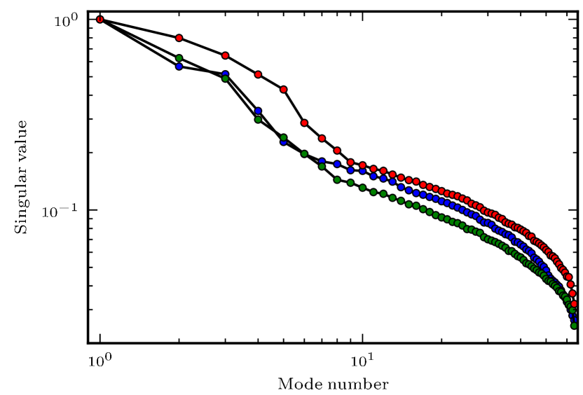
Figure 1: An example singular value spectrum for the three shortest baselines, each approximately 50–52 wavelengths at the zenith, with the largest singular value normalized to 1 for each.

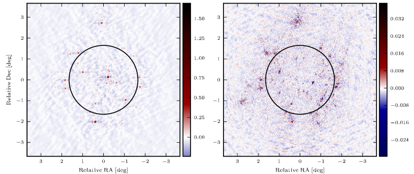
Figure 2: Sky image before and after an SVD foreground subtraction, for the night of 2007 December 10, using baselines up to 4 km. The colour scales are in units of Janskys and the black circle shows the full width half-maximum (FWHM) of the primary beam. The rms before any foreground removal (left) is 50 mJy. After removing eight SVD modes (right) the peak goes from 1.6 Jy to 39 mJy with an rms of 2 mJy. Residual point sources can still be seen around the edge of the beam while those within about one degree of the centre are effectively removed.

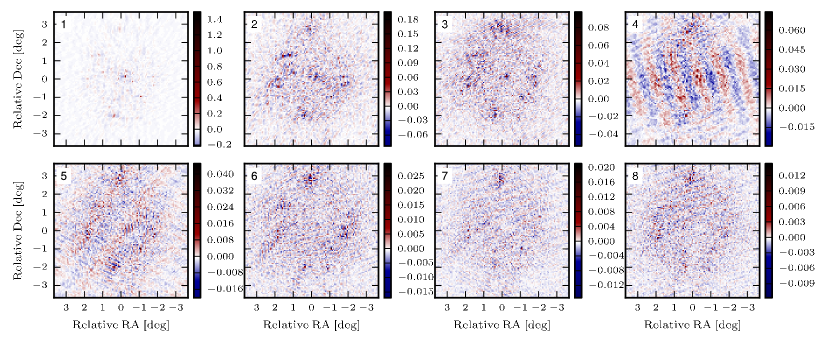
Figure 3: Sky images of the top eight SVD modes identified in the data from 2007 December 10, with all other modes set to zero. These modes are the ones subtracted between the two sky images in Fig. 2. The colour scales are in units of Janskys.

2 Observations and Data

The data analysed in this paper were taken over five nights in 2007 December and total about 40 h. The observations were centred on PSR B0823+26, a pulsar about 30^∘ off the Galactic plane, which is used to calibrate both the phases and the ionosphere by dividing the pulsar period into several gates and separating the on- and off-pulse gates. The primary beam has a full width half-maximum (FWHM) of 3.1^∘ and a maximum angular resolution of about 20 arcsec. The bandwidth covers a frequency range from 139.3 to 156.0 MHz in 64 frequency bins of 0.25 MHz each with a time resolution of 64 s. This corresponds to a redshift range of $z=8.1$–$9.2$. For more details on the observations, including radio frequency interference (RFI) removal strategies, see Paciga et al. (2011). The remainder of this section outlines the differences in the data analysis compared to this earlier work.

In addition to automated flagging of visibilities and the SVD RFI removal pipeline for broad-band interference, we have also added manual flagging of faulty antennas, timestamps, and frequency ranges that are exceptionally noisy or that visually appear to have RFI left after the automated procedures. Approximately 15 per cent of the visibilities are flagged in this way, while the dynamic range, defined as the ratio of the peak flux of the calibration source to the rms outside the primary beam, is improved by as much as a factor of 4.

To improve the comparability of each of the five nights of observing, we limit each night to the same LST range, and have regridded the visibilities in time such that each night shares the exact same timestamps, equally spaced in one minute intervals. Additionally, it is known that the flux of a pulsar can change significantly with time, which creates another source of variability from night to night. Since the visibilities are gated on the period of the pulsar, it can easily be subtracted from the data. These two changes reduce the rms noise in the difference between pairs of days by a factor of 2 on average.

Finally, the power spectrum is calculated from the cross-correlation of pairs of nights in annuli of $(u,v)$ space. This gives the 2D power perpendicular to the line of sight as a function of baseline length $|\mathbf{u}|$ or equivalently multipole moment $\ell=2\pi|\mathbf{u}|$. At the smallest $|\mathbf{u}|$, a bin width equal to that of the primary beam (20 wavelengths) was used. At larger $|\mathbf{u}|$, each bin width is increased by 60 per cent, to compensate for the decreasing density of visibilities.

It was found that outliers tended to skew the mean power in each annulus. Since the median is much more robust to such outliers, we calculate the power in each annulus (that is, at each angular scale $\ell$) as the median value over all frequencies. The error in each annulus is estimated as the median of the absolute deviations from the median power, weighted by the noise. The final power spectrum is the bootstrapped average of the power spectra over all 10 possible cross-correlation pairs of the 5 nights.

The power can also be expressed in terms of the wavenumber perpendicular to the line of sight, ${k_{\perp}}\approx(\ell/6608)\,h\,\mathrm{Mpc}^{-1}$, which becomes useful when discussing the 3D power. In the 2D case we will continue to use $\ell$. Since we do not yet include line-of-sight information, this is the power as a function of $\ell$ with fixed ${k_{\parallel}}=0$, which we denote $P(\ell|{k_{\parallel}}=0)$.

3 Foreground Removal

3.1 Singular Value Decomposition

Foreground removal techniques typically rely on the fact that the foreground signal is expected to be much smoother in frequency (that is, has fewer degrees of freedom) than the reionization signal, which decorrelates on the order of one to a few megahertz (Bharadwaj & Ali, 2005). Observations of foregrounds around 150 MHz with GMRT have shown that the fluctuations in frequency are large enough to make polynomial fits insufficient to model them (Ali et al., 2008; Ghosh et al., 2012). In this work, we instead use an SVD, which still isolates smooth foreground modes but does not make a priori assumptions that the foregrounds can be approximated with a particular function. A similar technique has been used by Chang et al. (2010) and Masui et al. (2012) to clean foregrounds for HI intensity mapping at $z\approx 0.8$, where the relative dominance of foregrounds over the 21 cm signal is comparable to $z\approx 8.6$. For reionization, Liu & Tegmark (2012) have developed a framework for using SVD modes of a frequency-frequency correlation matrix to clean foregrounds at MWA.

We perform an SVD for each baseline individually on the visibilities arranged in a matrix by time and frequency. The number of modes is limited by the 64 frequency channels. Fig. 1 shows the singular values for the shortest baselines. The spectra of values on a given baseline is generally consistent from day to day, but occasionally there are large jumps in both amplitude and rate of decline with mode number, which are likely due to either RFI or calibration errors. In these cases, the noise on the baseline also becomes much larger, such that in the final calculation of the power spectrum their contribution is significantly down-weighted.

A sky image using 8 h of data from a single night is shown in Fig. 2, compared with the same data after the first eight SVD modes, shown in Fig. 3, are removed. The overall flux is reduced substantially after only a few modes are removed. While the sources in the centre of the field are removed quite well, the dominant residuals are the point sources near the edge of the beam. This is generically true of any foreground subtraction used on this data set, as was also seen in Paciga et al. (2011). This is most likely due to beam edge effects, the worst residuals being close to the first null where the frequency dependence of the beam pattern is most significant. Though there are sophisticated schemes that may be able to model point sources while minimizing the impact on the 21 cm signal (e.g., Datta et al., 2010; Bernardi et al., 2011; Trott et al., 2012), at the angular scales we are interested in for this work ($\ell\la 2000$) the point sources are confusion limited and contribute in the same way as the diffuse background.

Each night goes through the SVD foreground removal separately, and then the cross-correlations are used to arrive at a power spectrum using the method described in section 2. The spectra for several numbers of SVD modes removed are shown in Fig. 4.

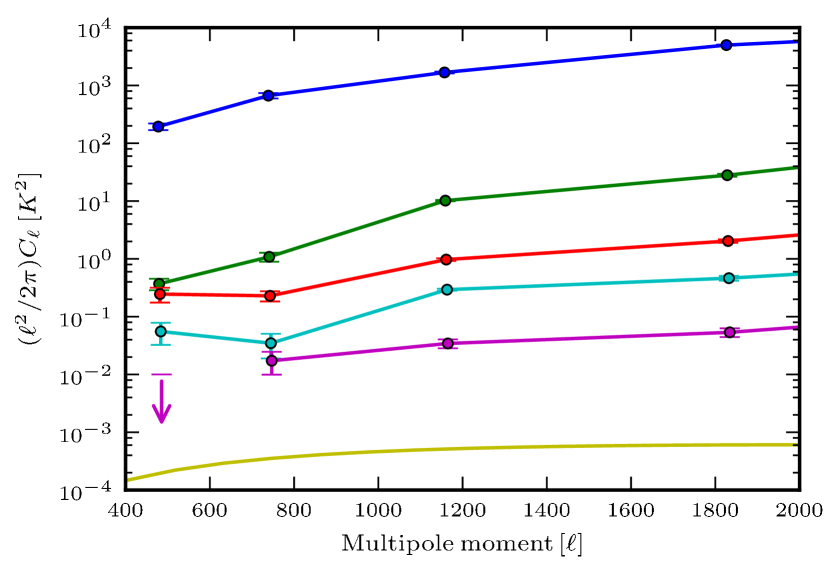
Figure 4: Power spectra before and after SVD mode removal. The blue line shows before any modes are removed. The green, red, cyan, and purple lines are for 4, 8, 16, and 32 modes removed, respectively. The error bars are from a bootstrap analysis of all cross-correlated pairs from the five nights of data. The solid yellow line represents the theoretical signal from Jelić et al. (2008).

3.2 Quantifying Signal Loss

A general problem with any foreground removal strategy is that it is impossible to completely separate the foregrounds from the signal, such that the foreground removal will likely remove some signal as well. Early work by Nityananda (2010) used a simple model of an SVD applied to a single visibility matrix to show that the signal loss could be calculated analytically. Our method of using an SVD for each baseline independently is more complex, and we wish to estimate the signal loss directly from the data itself. To quantify the signal loss, we aim to find the transfer function between the observed power $P_{\mathrm{SVD}}(\ell)$ and the real 21 cm power $P_{21\mathrm{cm}}(\ell)$. Since the real power is unknown, we use a simulated signal as a proxy. This is added to the data before the foreground subtraction and the resulting power spectrum after subtraction is compared to the input signal.

The simulated signal we use is a Gaussian random field with a matter overdensity power spectrum from CAMB scaled to $z=8.6$ using the linear-regime growth from $z=1.5$, and with the amplitude calibrated to be similar to the expected 21 cm signal from EoR assuming that the spin temperature is much greater than the CMB temperature. Fig. 5 is an image of the simulated signal as it would be seen by GMRT in the absence of any foregrounds or noise. The effect of the beam profile on the power spectrum is less than 3 per cent for scales in the range $40<\ell<2000$, and so has a relatively small effect on the result.

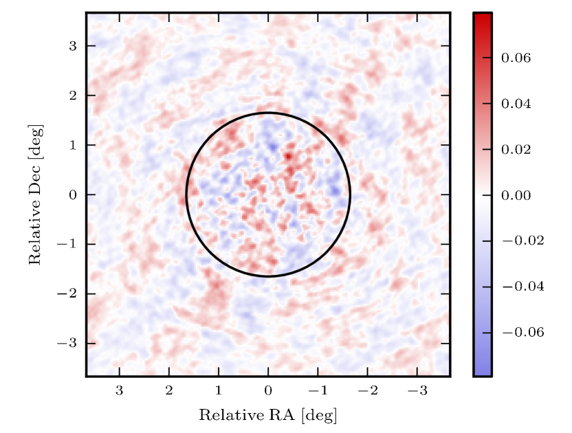
Figure 5: An image of the simulated signal as seen with GMRT in the absence of foregrounds or noise, using the same baselines and field of view as Fig.s 2 and 3. The colour scale is in units of mJy. The solid circle represents the FWHM of the primary beam.

Given a data set $x$ which is the sum of the observed data and a simulated signal, the transfer function $T(x\rightarrow F(x);\ell)$ measures how much of the signal survives in the foreground filtered data set $F(x)$ as a function of $\ell$. While $F(x)$ can stand in for any filter method applied to the visibilities $x$, for the SVD we must also specify that the modes removed are those calculated from the visibilities $x$ themselves. While the transfer function measures the signal loss for a single set of data, the power is measured from the cross-correlations of those data sets, so the relationship can be written as

$$P_{\mathrm{SVD}}(\ell)=T(x\rightarrow F(x);\ell)^{2}P_{21\mathrm{cm}}(\ell).$$ (1)

Unless it is necessary to be explicit about the mapping $T$ is measuring, we will shorten this notation to simply $T(\ell)$.

There are numerous ways one can estimate this function. The most direct way is to cross-correlate $F(x)$ with the injected signal, and normalize by the auto-power of that same signal. This is written as

$$T_{0}(\ell)=\frac{F(\textrm{data}+\textrm{signal})\times\textrm{signal}}{\textrm{signal}\times\textrm{signal}}.$$ (2)

In the ideal case where $F(x)$ removes foregrounds perfectly this will equal exactly 1.0. While conceptually simple, and used successfully by Masui et al. (2012) for data at $z\approx 0.8$, we find this estimator of the transfer function to be exceptionally noisy for realistic cases where $F(x)$ leaves residual foregrounds. In the case of the SVD, we would expect the function to become less noisy as more modes are removed and the residual foregrounds decrease, but we are still significantly limited in being able to measure the power.

An alternative is to subtract the original visibilities, under the same foreground filter, from the combined real and simulated visibilities before cross-correlating with the simulated signal. To distinguish it from the previous one, we denote this version of the transfer function $T_{1}$, which takes the form

$$T_{1}(\ell)=\frac{[F(\textrm{data}+\textrm{signal})-F(\textrm{data})]\times\textrm{signal}}{\textrm{signal}\times\textrm{signal}}.$$ (3)

In addition to being much less noisy when residual foregrounds are present, this has the benefit that by subtracting the original data we remove the possibility of the real 21 cm signal in the data correlating with the simulated signal and biasing the result. If $F(x)$ left the signal untouched, this would in principle be equal to 1.0. However, deviations are possible even when $F(x)=x$. This is due to the fact that the cross-correlations with real data in the numerator introduces RFI masks, noise, and day-to-day variations which are not present in the pure signal in the denominator. Thus, the transfer function will also correct for these effects, which enter at a level of a few per cent.

We carry out this process of estimating $T(\ell)$, averaging over 100 realizations of the simulated signal, after which both the mean and the standard deviation are well determined, and the error in the mean is small enough that it will not contribute significantly to the corrected power spectra later. Fig. 6 shows $T_{1}$ for a selection of SVD filters. While the transfer function in principle can depend non-linearly on the amplitude of the input signal, we find that the result does not change significantly within a factor of 10 of realistic signal temperatures. In the regimes where the transfer function does begin to depend on the input temperature, the two are anti-correlated; larger signals are more readily misidentified as foregrounds by the SVD, leading to a small value of $T(\ell)$.

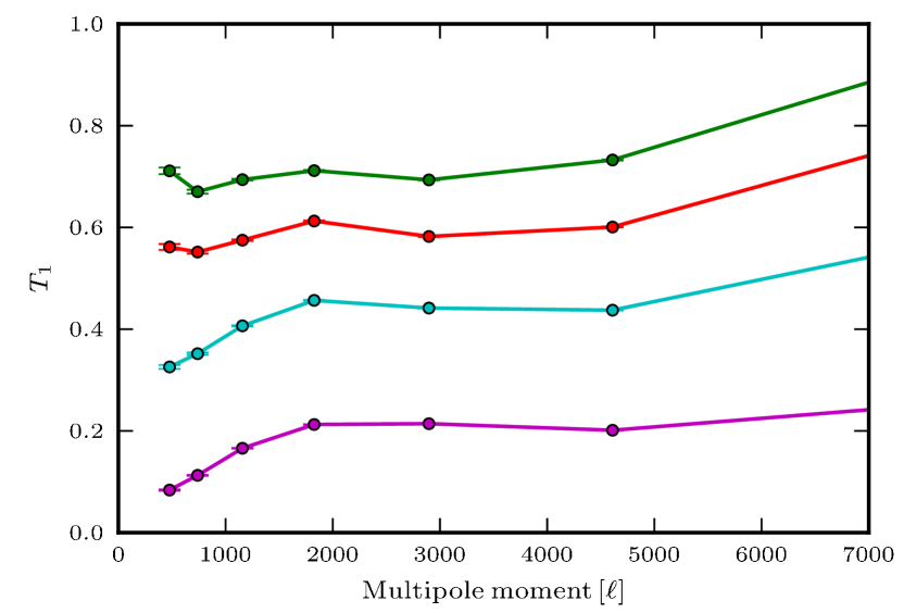
Figure 6: Transfer function $T_{1}$ with 4 (green), 8 (red), 16 (cyan), and 32 (purple) SVD modes removed, showing the fraction of the 21 cm signal that we estimate survives the SVD foreground removal. With only four modes removed, most of the 21 cm signal is expected to survive. However, when 32 modes are removed, about 20 per cent or less survives, depending on the angular scale.

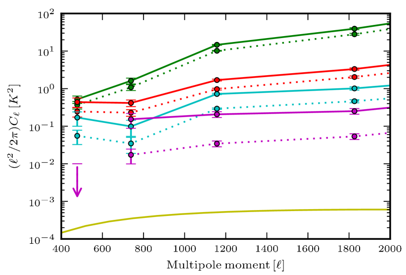
Figure 7: The $T_{1}$-corrected power spectra after SVD foreground removal. The colours represent 4 (green), 8 (red), 16 (cyan), and 32 (purple) SVD modes removed. The dotted lines show the uncorrected power spectra as in Fig. 4, while the solid lines show the power spectra after correcting for the transfer function. For 32 modes removed, at low $\ell$, the corrected power is larger than that for only 16 modes removed. As in Fig. 4, the solid yellow line represents the theoretical signal from Jelić et al. (2008).

The transfer function can be used to determine the best number of modes to remove, since as more modes are removed more of the 21 cm signal will be reduced to a point where the additional correction to the signal outweighs the gain from reducing the foregrounds. Fig. 7 shows that correcting for the transfer function after 32 modes are removed gives a weaker limit on the power than only removing 16 modes.

4 3D Power Spectrum

4.1 Line-of-sight power

The power calculated from annuli in visibility space only measures the 2D power perpendicular to the line of sight (that is, as a function of the multipole moment $\ell$ or wavenumber ${k_{\perp}}$). To find the full 3D power, we must also look at the line-of-sight, or frequency, direction and measure power as a function of ${k_{\parallel}}$. While certain forms of foreground filters will have a window function that naturally selects a ${k_{\parallel}}$, the SVD filter does not have a well defined behaviour along the line of sight. The gives us the flexibility of selecting the window function.

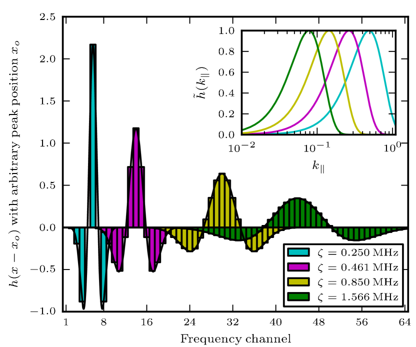
Figure 8: Hermite window in frequency space. Four examples are shown with different values of $\zeta$ increasing from left to right, with arbitrary horizontal offset. Bars indicate the value of the window in each frequency bin. In practice, $\zeta$ should not be smaller than the frequency resolution, limiting the ${k_{\parallel}}$ available. The inset plot shows the Fourier transform.

Hermite functions, having the benefit of zero mean and a simple Fourier transform, are well suited to select a range of ${k_{\parallel}}$. In frequency space, we define a window

$$h(\nu)=\frac{1}{\sqrt{8\pi}\zeta}\left(1-\frac{\nu^{2}}{\zeta^{2}}\right)\exp\left(1-\frac{\nu^{2}}{2\zeta^{2}}\right)$$ (4)

where $\zeta$ is a parameter analogous to the standard deviation of a Gaussian distribution, which in this case specifies the location of the zeros. This is shown in Fig. 8 for several $\zeta$ compared to the frequency bin size. This window has the Fourier transform

$$\tilde{h}({k_{\parallel}})=\frac{({k_{\parallel}}r\zeta)^{2}}{2}\exp\left[1-\frac{({k_{\parallel}}r\zeta)^{2}}{2}\right].$$ (5)

We have used the conversion factor $r\approx 11.6\,h^{-1}\mathrm{Mpc}/\mathrm{MHz}$ such that ${k_{\parallel}}$ is in units of $h\,\mathrm{Mpc}^{-1}$. The normalization has been chosen such that the maximum of $\tilde{h}({k_{\parallel}})$ is 1, thus preserving power. This peak in Fourier space, shown in the inset of Fig. 8, occurs when ${k_{\parallel}}=\sqrt{2}/(r\zeta)$ and determines the ${k_{\parallel}}$ at which most power survives the Hermite window. Larger $\zeta$ sample smaller ${k_{\parallel}}$, with the range of possible values limited by the frequency resolution and bandwidth.

4.2 Three approaches to the transfer function

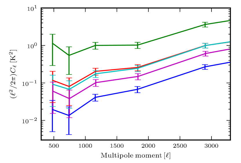
Figure 9: An example power spectrum at $\zeta=0.25$ MHz (${k_{\parallel}}=0.49\,h\,\mathrm{Mpc}^{-1}$) with 16 SVD modes removed (blue line), with the effect of each type of transfer function correction for $T_{1}$ shown. The green line corrects for both the Hermite window and the SVD subtraction, while the red line reintroduces the Hermite window, which agrees quite well with the semi-Hermite correction (cyan). The purple line uses the SVD-only transfer function. Error bars are from include contributions from the transfer function and the bootstrap error from the raw power spectra. In this example, the three approaches agree quite well, though they can diverge by an order of magnitude for other selections of mode subtraction and ${k_{\parallel}}$.

By applying a Hermite window to the data, we can calculate the 2D power spectrum at a fixed ${k_{\parallel}}$. There is some complication, however, in how we can use a transfer function to correct for possible signal loss. The Hermite filter by design reduces power on most scales while leaving power only at a specific ${k_{\parallel}}$, and we want the transfer function to only adjust for signal lost at the same ${k_{\parallel}}$. Ideally, one would apply the Hermite filter first to isolate the input power at the scales of interest and run the foreground filters on that data. If $H(x)$ represents the data set with a Hermite window applied, this would measure $T(H(x)\rightarrow F(H(x));\ell)$. Unfortunately, the SVD actually depends strongly on information in the ${k_{\parallel}}$ direction, which means that $F(H(x))$ may have a much different effect on the power at the chosen length scale than $F(x)$. That is to say, the Hermite and SVD operations do not commute.

There are several possible approaches to get around this, which are as follows:

1. Assume that the transfer function is not strongly dependent on ${k_{\parallel}}$, and use $T(x\rightarrow F(x);\ell)$ from the ${k_{\parallel}}=0$ case independent of the ${k_{\parallel}}$ selected by the Hermite window. We call this the ‘SVD only’ approach. The ${k_{\parallel}}$ behaviour only enters in through calculation of the power spectra after the Hermite window. Any important behaviour of the SVD in the ${k_{\parallel}}$ direction will not be captured.

2. We can calculate a transfer function for the signal loss due to the total effect of both the Hermite window and the SVD, $T(x\rightarrow H(F(x));\ell)$, and correct for both. We can then use an analytical form for the transfer function of the Hermite window alone to reintroduce the scale window and keep only the power at our selected ${k_{\parallel}}$. We call this the ‘full Hermite’ approach.

   To find its analytical form, we start with the fact that the transfer function associated with the Hermite window measures the ratio of the windowed power to the full power,

   $$T_{H}^{2}({k_{\perp}})=\frac{\int P({k_{\perp}},{k_{\parallel}})|\tilde{h}({k_{\parallel}})|^{2}\mathrm{d}{k_{\parallel}}}{\int P({k_{\perp}},{k_{\parallel}})\mathrm{d}{k_{\parallel}}}.$$ (6)

   If we assume the power spectrum has the form

   $$P({k_{\parallel}})\propto\frac{1}{{k_{\parallel}}^{2}+{k_{\perp}}^{2}}$$ (7)

   both the numerator and denominator of this can be evaluated analytically. The result is

   $$T_{H}^{2}({k_{\perp}}) = \frac{e^{2}r\zeta{k_{\perp}}}{8\sqrt{\pi}}\left(1-2r^{2}\zeta^{2}{k_{\perp}}^{2}\phantom{e^{r^{2}\zeta^{2}{k_{\perp}}^{2}}}\right.$$ (8)

   $$\left.+2\sqrt{\pi}r^{3}\zeta^{3}{k_{\perp}}^{3}e^{r^{2}\zeta^{2}{k_{\perp}}^{2}}\mathrm{erfc}[r\zeta{k_{\perp}}]\right)$$

   where $\mathrm{erfc}[x]=1-\mathrm{erf}[x]$ is the complimentary error function. Requiring the most steps, this method has more avenues to introduce errors or biases.

3. Apply the Hermite window first to the simulated signal. When added to the full data and passed through the SVD foreground removal, the larger amplitude of the foregrounds present in the data ensures that the SVD still has data at all ${k_{\parallel}}$ to operate on. However, since there is only a simulated signal at a specific ${k_{\parallel}}$, the cross-correlation with the simulated signal when calculating the transfer function $T(\mathrm{data}+H(\mathrm{signal})\rightarrow F(\mathrm{data}+H(\mathrm{signal}));\ell)$ only measures the effect of the SVD on that ${k_{\parallel}}$. We call this the ‘semi-Hermite’ approach. This assumes that the SVD as applied to the ${k_{\parallel}}$ limited simulated signal is a suitable proxy for how the SVD affects the real signal, given that both the real signal and the ${k_{\parallel}}$ limited simulated signal are of significantly lower amplitude than the foregrounds.

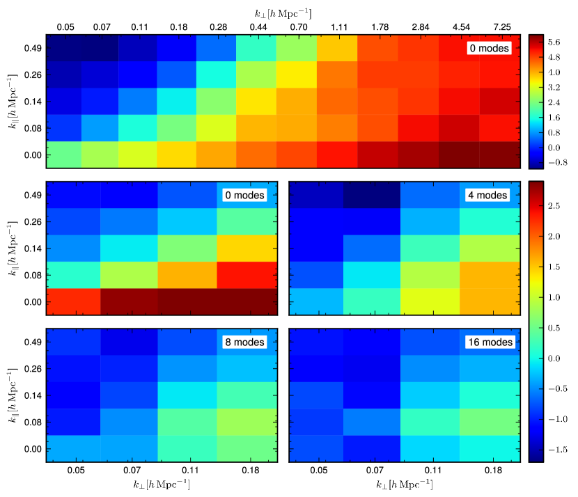
Figure 10: Power spectra as a function of both ${k_{\perp}}$ and ${k_{\parallel}}$ corrected with $T_{1}$ calculated using the semi-Hermite approach. The topmost plot shows the entire ${k_{\perp}}$ range without any foreground removal. The four smaller plots show 0, 4, 8, and 16 SVD modes removed on the same colour scale for only the lowest few ${k_{\perp}}$ bins. The colour scales are in units of $\log(\mathrm{K^{2}})$. Compared to the case with 0 modes removed, the SVD tends to reduce the overall power by one to three orders of magnitude. See also Fig. 11, which shows the power as a function of the total $k$.

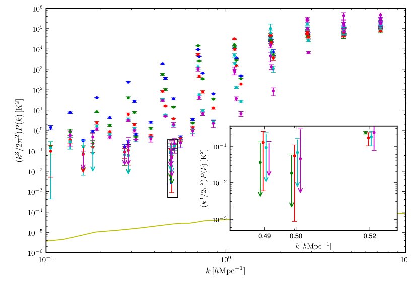
Figure 11: Power as a function of the total wavenumber $k=\sqrt{{k_{\perp}}^{2}+{k_{\parallel}}^{2}}$. Each point represents a different $({k_{\perp}},{k_{\parallel}})$ pair; there is no binning in $k$. Colours indicate the number of SVD modes removed; 0 (blue), 4 (green), 8 (red), 16 (cyan), and 32 (purple) are shown. The boxed region at $k\approx 0.5$ is shown inset, with nearby points each of the three marked $k$ spread out slightly for clarity. The best limit at $2\sigma$ is (248 mK)² at 0.50 $h$Mpc^-1 achieved with four SVD modes removed. The solid line shows the predicted 3D power spectrum from Iliev et al. (2008) assuming a 30 mK signal.

Fig. 9 shows a typical power spectrum for a particular choice of SVD filter, transfer function, and ${k_{\parallel}}$, without any correction and the resulting spectra after each of the above approaches. Differences in each approach illustrate the difficulty in finding an unbiased estimator that gives a robust result.

We find that in both the full Hermite and semi-Hermite methods there is a ${k_{\parallel}}$ dependence which is not captured by the SVD-only method, which is constant with ${k_{\parallel}}$ by definition. All three methods show deviations from unity of the order of a few per cent with zero SVD modes removed due to the additional effects from RFI masking, noise, and the beam that are captured by the transfer function. It is notable, however, that the ‘full Hermite’ approach finds $T_{1}$ deviating from 1 by tens of percent in some regimes, especially at low ${k_{\perp}}$. This is likely indicative of a mismatch between the amount of power being removed by the combination of SVD and Hermite filters and the amount modelled by the analytic form. This suggests that in areas of $({k_{\perp}},{k_{\parallel}})$ space where $T_{1}>1$, this method may overestimate the amount of signal present, in turn underestimating the 21 cm power by failing to fully correct for the signal loss. None the less, the full and semi-Hermite approaches agree much better with more SVD modes removed. Since the semi-Hermite approach seems to capture both the ${k_{\parallel}}$ dependence and is relatively well behaved with $0<T_{1}<1$, we use it as the canonical transfer function.

4.3 Sampling $({k_{\perp}},{k_{\parallel}})$ space to get $P(k)$

Using the Hermite window to select a fixed ${k_{\parallel}}$ allows us to calculate $P(\ell|{k_{\parallel}})$ and the associated transfer function at that ${k_{\parallel}}$. By repeating this for a series of ${k_{\parallel}}$, we can build up the full 3D power spectrum.

Fig. 10 shows the power as a function of both ${k_{\perp}}$ and ${k_{\parallel}}$ using the semi-Hermite correction, given a series of different SVD mode subtractions. The power shows a pattern of lower values towards low ${k_{\perp}}$ and high ${k_{\parallel}}$. Fig. 11 shows the same measurements as a function of the 3D wavenumber $k=\sqrt{{k_{\perp}}^{2}+{k_{\parallel}}^{2}}$. Though the SVD is our primary mode of foreground removal, the Hermite function itself acts as a foreground filter removing the large-scale structure in frequency space. This is reflected in the points where zero SVD modes have been removed. It is clear that our ability to remove foregrounds drops off quickly above about $k\approx 0.5\,h\,\mathrm{Mpc}^{-1}$. Our best limit at $2\sigma$ is $(248\,\mathrm{mK})^{2}$, achieved at $({k_{\perp}},{k_{\parallel}})=(0.11,0.49)\,h\,\mathrm{Mpc}^{-1}$, or a total $k$ of $0.50\,h\,\mathrm{Mpc}^{-1}$, with four SVD modes removed. At this point, the semi-Hermite value of the transfer function was $T_{1}=0.74$, meaning that an estimated 26 per cent of signal was removed by the SVD mode subtraction and Hermite window operating on each day in the cross-correlations. If instead 16 modes are removed, the limit changes to $(319\,\mathrm{mK})^{2}$ but 55 per cent of the signal is lost. Any residual foregrounds, though reduced by a much larger fraction than the signal, will also have been boosted by this correction, making this measurement an upper limit on the actual 21 cm signal.

5 Conclusion

Using an SVD as a foreground removal technique and a simulated signal to quantify the loss of a real 21 cm signal the SVD may cause, we have calculated an upper limit to the HI power spectrum at $z=8.6$ of (248 mK)² at $k=0.50\,h\,\mathrm{Mpc}^{-1}$. The ${k_{\perp}}$ component was found using the median power in annuli of the $(u,v)$ plane, while a Hermite window was used to sample the ${k_{\parallel}}$ direction. This is in contrast to our previous work with a piecewise-linear filter which operated only in the frequency direction and carried with it an implicit ${k_{\parallel}}$ window.

This limit is dependent on the method one chooses to calculate the transfer function between the real 21 cm signal and the observed power. Both the ${k_{\perp}}$ and ${k_{\parallel}}$ behaviour of the foreground filter chosen needs to be taken into account. While the semi-Hermite method chosen uses a simulated signal with power in a limited ${k_{\parallel}}$ window, and may miss interactions between the SVD filter and the signal over larger ${k_{\parallel}}$ bands, we believe it to give the most reliable estimate of the transfer function and a suitably conservative estimate on the final upper limit.

Had we instead used the full Hermite approach described, this limit would have been $(260\,\mathrm{mK})^{2}$. That this second approach gives a similar value suggests that this limit is a fairly robust one. The difference can likely be attributed in part to the simplifying assumptions necessary when deriving the analytical Hermite windowing function. We also consider the current result to be more robust than that reported previously in Paciga et al. (2011). While the previous limit was considerably lower, this can be accounted for by many factors; the different $k$ scale, the change in foreground filter, several minor changes in the analysis pipeline detailed in section 2 and most significantly the fact that this is the first time a transfer function has been used to correct for signal lost in the foreground filter. Without such a correction, our best upper limits with the SVD foreground filter may have been incorrectly reported as low as (50 mK)².

This limit still compares favourably to others established in the literature which are of the order of several Kelvin (e.g., Bebbington, 1986; Ali et al., 2008; Parsons et al., 2010). Recently, after submission of our paper, PAPER (Parsons et al., 2013) claimed an upper limit of (52 mK)² at $k=0.11\,h\,\mathrm{Mpc}^{-1}$ and $z=7.7$. However, it is not documented whether signal loss from their primary foreground filtering step (their section 3.4) has been accounted for and so it is not clear how to compare their result to ours. LOFAR has begun publishing initial results from reionization observations, but have so far focused on much longer scales ($\ell\approx 7500$) (Yatawatta et al., 2013).

In Paciga et al. (2011) we considered a model with a cold intergalactic medium (IGM), a neutral fraction of 0.5 and fully ionized bubbles with uniform radii. In such a model this current limit would constrain the brightness temperature of the neutral IGM to be at least 540 mK in absorption against the CMB. However, a value of the HI power spectrum of (248 mK)² is almost an order of magnitude higher than what is generally considered physically plausible in most reionization models. In particular, this result does not constrain reionization models with a warm IGM where the spin temperature is much greater than the CMB temperature.

The SVD procedure could be refined further by a baseline-by-baseline accounting of the optimal number of modes to subtract or by limiting the field of view on the sky to the innermost area of the beam where point source residuals are minimal, although it is not obvious what effect this would have on the signal at small angular scales. Making a measurement at larger $\ell$ would require a more careful treatment of point sources but is also limited by the fact that the SVD is less effective for longer baselines. Regardless of the foreground removal technique used, it is likely that accurately correcting for the any resulting loss of the 21 cm signal, and disentangling the 21 cm signal from any residual foregrounds, will remain a significant challenge in measuring the true EoR power spectrum.

6 Acknowledgements

Special thanks to Eric Switzer and Kiyoshi Masui for many useful discussions during the preparation of this work. We thank the staff of the GMRT that made these observations possible. GMRT is run by the National Centre for Radio Astrophysics of the Tata Institute of Fundamental Research. The computations were performed on CITA’s Sunnyvale clusters which are funded by the Canada Foundation for Innovation, the Ontario Innovation Trust and the Ontario Research Fund. The work of GP, UP and KS is supported by the Natural Science and Engineering Research Council of Canada. KB, JP and TV are supported by NSF grant AST-1009615.

References

- Ali et al. (2008) Ali S. S., Bharadwaj S., Chengalur J. N., 2008, MNRAS, 385, 2166
- Ananthakrishnan (1995) Ananthakrishnan S., 1995, Journal of Astrophysics and Astronomy Supplement, 16, 427
- Beardsley et al. (2013) Beardsley A. P. et al., 2013, MNRAS, 429, L5
- Bebbington (1986) Bebbington D. H. O., 1986, MNRAS, 218, 577
- Becker et al. (2001) Becker R. H. et al. 2001, AJ, 122, 2850
- Bernardi et al. (2011) Bernardi G., Mitchell D. A., Ord S. M., Greenhill L. J., Pindor B., Wayth R. B., Wyithe J. S. B., 2011, MNRAS, 413, 411
- Bharadwaj & Ali (2005) Bharadwaj S., Ali S. S., 2005, MNRAS, 356, 1519
- Bowman & Rogers (2010) Bowman J. D., Rogers A. E. E., 2010, Nature, 468, 796
- Bowman et al. (2008) Bowman J. D., Rogers A. E. E., Hewitt J. N., 2008, ApJ, 676, 1
- Brentjens et al. (2011) Brentjens M., Koopmans L. V. E., de Bruyn A. G., Zaroubi S., 2011, in American Astronomical Society Meeting Abstracts #217 Vol. 43 of Bulletin of the American Astronomical Society, The Low-Frequency Array (LOFAR) and EoR Key-Science Project. p. #107.04
- Carilli et al. (2004) Carilli C. L., Furlanetto S., Briggs F., Jarvis M., Rawlings S., Falcke H., 2004, New Astron. Rev., 48, 1029
- Chang et al. (2010) Chang T.-C., Pen U.-L., Bandura K., Peterson J. B., 2010, Nature, 466, 463
- Chapman et al. (2012) Chapman E. el al., 2012, MNRAS, 423, 2518
- Cooray et al. (2008) Cooray A., Li C., Melchiorri A., 2008, Phys. Rev. D, 77, 103506
- Datta et al. (2010) Datta A., Bowman J. D., Carilli C. L., 2010, ApJ, 724, 526
- Datta et al. (2012) Datta K. K., Friedrich M. M., Mellema G., Iliev I. T., Shapiro P. R., 2012, MNRAS, 424, 762
- de Oliveira-Costa et al. (2008) de Oliveira-Costa A., Tegmark M., Gaensler B. M., Jonas J., Landecker T. L., Reich P., 2008, MNRAS, 388, 247
- Dillon et al. (2013) Dillon J. S., Liu A., Tegmark M., 2013, Phys. Rev.D, 87, 43005
- Djorgovski et al. (2001) Djorgovski S. G., Castro S., Stern D., Mahabal A. A., 2001, ApJl, 560, L5
- Friedrich et al. (2011) Friedrich M. M., Mellema G., Alvarez M. A., Shapiro P. R., Iliev I. T., 2011, MNRAS, 413, 1353
- Furlanetto et al. (2009) Furlanetto S. R. et al. 2009, Astro2010: The Astronomy and Astrophysics Decadal Survey, Science White Papers, 82
- Furlanetto et al. (2006) Furlanetto S. R., Oh S. P., Briggs F. H., 2006, Phys. Rep., 433, 181
- Furlanetto et al. (2006) Furlanetto S. R., Oh S. P., Pierpaoli E., 2006, Phys. Rev. D, 74, 103502
- Furlanetto et al. (2004) Furlanetto S. R., Zaldarriaga M., Hernquist L., 2004, ApJ, 613, 1
- Ghosh et al. (2012) Ghosh A., Prasad J., Bharadwaj S., Ali S. S., Chengalur J. N., 2012, MNRAS, 426, 3295
- Griffen et al. (2013) Griffen B. F., Drinkwater M. J., Iliev I. T., Thomas P. A., Mellema G., 2013, MNRAS, 431, 3087
- Gunn & Peterson (1965) Gunn J. E., Peterson B. A., 1965, ApJ, 142, 1633
- Haiman (2011) Haiman Z., 2011, Nature, 472, 47
- Harker et al. (2010) Harker G. et al., 2010, MNRAS, 405, 2492
- Iliev et al. (2008) Iliev I. T., Mellema G., Pen U.-L., Bond J. R., Shapiro P. R., 2008, MNRAS, 384, 863
- Iliev et al. (2012) Iliev I. T., Mellema G., Shapiro P. R., Pen U.-L., Mao Y., Koda J., Ahn K., 2012, MNRAS, 423, 2222
- Jelić et al. (2008) Jelić V. et al., 2008, MNRAS, 389, 1319
- Komatsu et al. (2011) Komatsu E., Smith K. M., Dunkley J., et al. 2011, ApJS, 192, 18
- Kovetz & Kamionkowski (2013) Kovetz E. D., Kamionkowski M., 2013, Phys. Rev. D, 87, 63516
- Liu & Tegmark (2011) Liu A., Tegmark M., 2011, Phys. Rev. D, 83, 103006
- Liu & Tegmark (2012) Liu A., Tegmark M., 2012, MNRAS, 419, 3491
- Lonsdale et al. (2009) Lonsdale C. J., Cappallo R. J., Morales M. F., et al. 2009, IEEE Proceedings, 97, 1497
- Majumdar et al. (2012) Majumdar S., Bharadwaj S., Choudhury T. R., 2012, MNRAS, 426, 3178
- Mao et al. (2008) Mao Y., Tegmark M., McQuinn M., Zaldarriaga M., Zahn O., 2008, Phys. Rev. D, 78, 023529
- Masui et al. (2012) Masui K. W. et al., 2013, ApJL, 763, L20
- McGreer et al. (2011) McGreer I. D., Mesinger A., Fan X., 2011, MNRAS, 415, 3237
- McQuinn et al. (2007) McQuinn M., Lidz A., Zahn O., Dutta S., Hernquist L., Zaldarriaga M., 2007, MNRAS, 377, 1043
- McQuinn et al. (2006) McQuinn M., Zahn O., Zaldarriaga M., Hernquist L., Furlanetto S. R., 2006, ApJ, 653, 815
- Nityananda (2010) Nityananda R., 2010, NCRA Technical Report, http://ncralib1.ncra.tifr.res.in:8080/jspui/handle/2301/484
- Oh & Mack (2003) Oh S. P., Mack K. J., 2003, MNRAS, 346, 871
- Paciga et al. (2011) Paciga G. et al., 2011, MNRAS, 413, 1174
- Pandolfi et al. (2011) Pandolfi S., Ferrara A., Choudhury T. R., Melchiorri A., Mitra S., 2011, Phys. Rev. D, 84, 123522
- Parsons et al. (2012) Parsons A., Pober J., McQuinn M., Jacobs D., Aguirre J., 2012, ApJ, 753, 81
- Parsons et al. (2010) Parsons A. R. et al., 2010, AJ, 139, 1468
- Parsons et al. (2012) Parsons A. R., Pober J. C., Aguirre J. E., Carilli C. L., Jacobs D. C., Moore D. F., 2012, ApJ, 756, 165
- Parsons et al. (2013) Parsons A. R. et al., 2013, preprint (astro-ph/astro-ph/1208.0331v2)
- Petrovic & Oh (2011) Petrovic N., Oh S. P., 2011, MNRAS, 413, 2103
- Rawlings & Schilizzi (2011) Rawlings S., Schilizzi R., 2011, preprint (astro-ph/1105.5953)
- Schroeder et al. (2012) Schroeder J., Mesinger A., Haiman Z., 2012, MNRAS, p. 203
- Su et al. (2011) Su M., Yadav A. P. S., McQuinn M., Yoo J., Zaldarriaga M., 2011, preprint (astro-ph/1106.4313)
- Swarup et al. (1991) Swarup G., Ananthakrishnan S., Kapahi V. K., Rao A. P., Subrahmanya C. R., Kulkarni V. K., 1991, Current Science, Vol. 60, NO.2/JAN25, P. 95, 1991, 60, 95
- Trott et al. (2012) Trott C. M., Wayth R. B., Tingay S. J., 2012, ApJ, 757, 101
- Yatawatta et al. (2013) Yatawatta S. et al., 2013, A&A, 550, A136
- Zahn et al. (2007) Zahn O., Lidz A., McQuinn M., Dutta S., 2007, ApJ, 654, 12
- Zahn et al. (2012) Zahn O., Reichardt C. L., Shaw L., et al. 2012, ApJ, 756, 65
- Zaroubi et al. (2012) Zaroubi S., de Bruyn A. G., Harker G., et al. 2012, MNRAS, 425, 2964