$\mathcal{N}=2$ Theories from Cluster Algebras

Abstract

We propose a new description of 3d $\mathcal{N}=2$ theories which do not admit conventional Lagrangians. Given a quiver $Q$ and a mutation sequence $\bm{m}$ on it, we define a 3d $\mathcal{N}=2$ theory $\mathcal{T}[(Q,\bm{m})]$ in such a way that the $S^{3}_{b}$ partition function of the theory coincides with the cluster partition function defined from the pair $(Q,\bm{m})$.

Our formalism includes the case where 3d $\mathcal{N}=2$ theories arise from the compactification of the 6d $(2,0)$ $A_{N-1}$ theory on a large class of 3-manifolds $M$, including complements of arbitrary links in $S^{3}$. In this case the quiver is defined from a 2d ideal triangulation, the mutation sequence represents an element of the mapping class group, and the 3-manifold is equipped with a canonical ideal triangulation. Our partition function then coincides with that of the holomorphic part of the $SL(N)$ Chern–Simons partition function on $M$.

B10, B16, B34

1 Introduction

It has recently been discovered Terashima:2011qi ; Dimofte:2011ju ; Cecotti:2011iy (see also earlier works Drukker:2010jp ; Dimofte:2010tz ; Hosomichi:2010vh ) that there exists a beautiful correspondence (“3d/3d correspondence”) between the physics of 3d $\mathcal{N}=2$ gauge theories and the geometry of 3-manifolds. The latter, in more physical language, is the study of analytic continuation of 3d pure Chern–Simons $SU(2)$ gauge theory into a non-compact gauge group $SL(2)$ Witten:1989ip ; Witten:2010cx . More quantitatively, one of the consequences of this correspondence is that given a 3-manifold $M$ there is a corresponding 3d $\mathcal{N}=2$ theory $\mathcal{T}[M]$ such that the partition functions of the two theories coincide Terashima:2011qi :

$$Z^{\textrm{3d }\mathcal{N}=2}_{\mathcal{T}[M]}[S^{3}_{b}]=Z^{\textrm{Chern--Simons}}[M]\ ,$$ (1.1)

where the left-hand side is the 3-sphere partition function Kapustin:2009kz ; Jafferis:2010un ; Hama:2010av with a 1-parameter deformation by $b$ Hama:2011ea , and the right-hand side is the holomorphic part of the $SL(2)$ Chern–Simons theory with level $t$. The two parameters $b$ and $t$ are related by $b^{2}\sim 1/t$.

The correspondence (1.1) provides a fresh perspective on the systematic study of a large class of 3d $\mathcal{N}=2$ theories, and relations between them. An arbitrary hyperbolic 3-manifold could be constructed by gluing ideal tetrahedra, and correspondingly we could construct complicated 3d $\mathcal{N}=2$ theories starting from free $\mathcal{N}=2$ chiral multiplets. Gluing ideal tetrahedra is translated into the gauging of the global symmetries, and the change of polarization into an $Sp(2N,\mathbb{Z})$ action Kapustin:1999ha ; Witten:2003ya on 3d $\mathcal{N}=2$ theories. The 2-3 Pachner move, which represents the change of the ideal triangulation of the 3-manifold, is translated into the 3d $\mathcal{N}=2$ mirror symmetry Dimofte:2011ju .

Despite the beauty of this correspondence, we should keep in mind limitations of the correspondence (1.1) — not all 3d $\mathcal{N}=2$ theories are of the form $\mathcal{T}[M]$. The natural question is whether we can generalize the correspondence to a larger class of 3d $\mathcal{N}=2$ theories beyond those associated with 3-manifolds, or more generally whether there are any geometric structures in the “landscape” or “theory space” of 3d $\mathcal{N}=2$ theories. To answer these questions it is crucial to extract the essential ingredients from the correspondence (1.1).

Our answer to this question is that it is the mathematical structures of quiver mutations and cluster algebras which are essential for the correspondence (1.1). We study 3d $\mathcal{N}=2$ gauge theories $\mathcal{T}[M]$ for a large class of hyperbolic 3-manifolds, including arbitrary link complements in $S^{3}$. The present paper generalizes the previous works on this subject by the authors Terashima:2011qi ; Terashima:2011xe , and is a companion to the previous paper with K. Nagao Nagao:2011aa . It is also closely related to Cecotti:2011iy (see also Cecotti:2010fi ; Cordova:2012xk ).

Our approach turns out to be much more general than (1.1), and includes theories associated with $SL(N)$ Chern–Simons theories on 3-manifolds (cf. FockGoncharovHigher ), or more general theories not associated with 3-manifolds (Figure 1). We define a 3d $\mathcal{N}=2$ theory $\mathcal{T}[(Q,\bm{m})]$ for a pair of a quiver $Q$ and a mutation sequence $\bm{m}$ on it, satisfying the relation

$$Z^{\textrm{3d }\mathcal{N}=2}_{\mathcal{T}[(Q,\bm{m})]}[S^{3}_{b}]=Z^{\rm cluster}_{(Q,\bm{m})}\ ,$$ (1.2)

where the right-hand side is the cluster partition function defined in this paper. The right-hand side contains a quantum parameter $q$, which is related to the parameter $b$ on the left-hand side by the relation (2.6). We can think of the pair $(Q,\bm{m})$ as the defining data specifying the matter contents of 3d $\mathcal{N}=2$ theories, which in general do not have Lagrangian descriptions. It will be an exciting possibility to explore the properties of these theories further.

Figure 1: The class of 3d $\mathcal{N}=2$ theories (denoted by $\mathcal{T}[(Q,\bm{m})]$) is a special subset of general 3d $\mathcal{N}=2$ theories, and is large enough to contain theories $\mathcal{T}[M]$ dual to the geometry 3-manifolds. Little is known at present about the detailed properties of the theories $\mathcal{T}[(Q,\bm{m})]$, when the theory cannot be written in the form $\mathcal{T}[M]$.

Summary

The results of this paper are summarized as follows (Figure 2):

1. We introduce a new combinatorial object, a mutation network (section 2.3), which encodes the combinatorial data of a quiver $Q$ and a mutation sequence $\bm{m}$.

2. We obtain an explicit integral expression for the cluster partition function $Z^{\rm cluster}_{(Q,\bm{m})}$ associated with a mutation network (section 2.2, in particular (2.28)).

3. We outline the construction of a 3d $\mathcal{N}=2$ theory $\mathcal{T}[(Q,\bm{m})]$ whose $S^{3}_{b}$ partition function coincides with the partition function $Z^{\rm cluster}_{(Q,\bm{m})}$ defined previously from the mutation network (1.2) (section 3.2).

4. In this formulation we find that cluster $x$-variables (as opposed to $y$-variables commonly used in the literature in connection with 3-manifolds) nicely parametrize the global symmetry of the theory.

We also apply our formalism to the quivers and mutations associated with 3-manifolds, re-deriving and generalizing the previous results from a unified framework:

1. When the pair $(Q,\bm{m})$ satisfies certain conditions, we can construct an associated mapping cylinder $(\Sigma,\varphi)$ with a canonical ideal triangulation determined from $(Q,\bm{m})$ (section 4.3).

2. By appropriately identifying boundaries of the mapping cylinder $(\Sigma,\varphi)$, we obtain a large class of hyperbolic link complements, including arbitrary link complements in $S^{3}$ (section 4.4). This operation has a counterpart in the mutation network as well as the partition function.

3. We consider dimensional reduction of our 3d $\mathcal{N}=2$ theory to 2d $\mathcal{N}=(2,2)$ theory. The twisted superpotential coincides with the Neumann–Zagier potential NeumannZagier of hyperbolic geometry, and the vacuum equations of the 2d $\mathcal{N}=(2,2)$ theory reproduce the gluing equations of hyperbolic tetrahedra.

Note that our method is different from the existing results in the literature (e.g. Dimofte:2011ju ). Our approach relies on the Heegaard-like decomposition of 3-manifolds. This has the advantage of making the connections with the braid group and the mapping class group more direct. We also point out that cluster $x$-variables, in addition to the cluster $y$-variables discussed in the literature, play crucial roles in the construction of 3d $\mathcal{N}=2$ theories.

Figure 2: Schematic summary of this paper.

The rest of this paper is organized as follows. In section 2 we derive an integral expression of our partition functions, based on the formalism of quiver mutations and cluster algebras. The combinatorial data is summarized in the mutation network. We also write down the associated cluster partition function. In section 3 we study the 3d $\mathcal{N}=2$ theory associated with a mutation network. In section 4 we explain the geometry of hyperbolic 3-manifolds and their ideal triangulations, associated with a mutation network satisfying certain conditions. The final section (section 5) summarizes the results and comments on open problems. We include three appendices. Appendix A summarizes the properties of the quantum dilogarithm function used in the main text. Appendix B summarizes hyperbolic ideal triangulations and gluing equations. Appendix C explains the effect of the Dehn twist on the triangulation.

We have tried to make the paper accessible to a wide spectrum of readers, including mathematicians. In fact, most of the material in sections 2 and 4 (apart from the examples in section 4.6) require little prior knowledge of the subject (in physics or in mathematics), and no knowledge of supersymmetric gauge theories are necessary until section 3. Readers not interested in 3-manifold cases can skip section 4.

2 Quivers and Clusters

In this section we define the Hilbert space $\mathcal{H}_{Q}$ associated with a quiver $Q$, and the action of the mutations $\bm{m}$ on $\mathcal{H}_{Q}$. We also define the associated cluster partition function $Z^{\rm cluster}_{(Q,\bm{m})}$, and derive its integral expression. This section will be formulated in terms of quiver mutations and cluster algebras FominZelevinsky1 (see KellerSurvey for an introduction).

2.1 Quiver Mutations and Cluster Algebras

Let us begin with a quiver $Q$, i.e., a finite oriented graph. We denote the set of the vertices of the quiver by $I$, and its elements by $i,j,\ldots\in I$.

In this paper, we always assume that a quiver has no loops and oriented $2$-cycles (see Figure 3).

Figure 3: A loop (left) and an oriented $2$-cycle (right) of a quiver.

For vertices $i,j\in I$, we define

$$Q_{i,j}:=\#\{\text{arrows from $i$ to $j$}\}-\#\{\text{arrows from $j$ to $i$}\}\ ,$$ (2.1)

i.e., $|Q_{i,j}|$ represents the number of arrows from the vertex $i$ to $j$, and the sign represents the chirality (orientation) of the arrow. Note that the quiver $Q$ is uniquely determined by the matrix $Q_{i,j}$ under the assumptions above.

Given a vertex $k$, we define a new quiver $\mu_{k}Q$ (mutation of $Q$ at vertex $k$) by

$$(\mu_{k}Q)_{i,j}:=\begin{cases}-Q_{i,j}&\text{($i=k$ or $j=k$)}\ ,\\ Q_{i,j}+[Q{}_{i,k}]_{+}[Q_{k,j}]_{+}-[Q_{j,k}]_{+}[Q_{k,i}]_{+}&\text{$(i,j\neq k$)}\ ,\end{cases}$$ (2.2)

where we used the notation

$$[x]_{+}:=\textrm{max}(x,0)\ .$$ (2.3)

In more physical language, this can be regarded as a somewhat abstract version of the Seiberg duality Seiberg:1994pq . However, the difference here is that our mutations in general are outside the conformal window.

Let us now construct a non-commutative algebra $\mathcal{A}_{Q}$ associated with the quiver $Q$. This is generated by a set of variables $\mathsf{y}_{i}$, associated with each edge $i$, satisfying the relation

$$\mathcal{A}_{Q}:=\{\mathsf{y}_{i}\,{}_{(i\in I)}\,|\,\mathsf{y}_{j}\mathsf{y}_{i}=q^{2Q_{i,j}}\mathsf{y}_{i}\mathsf{y}_{j}\}\ ,$$ (2.5)

where $q$ is the quantization parameter which is related to the parameter $b$ by

$$q=e^{\sqrt{-1}\pi b^{2}}\ .$$ (2.6)

This parameter $b$ will later be identified with the deformation parameter of $S^{3}$ in (1.1). The semiclassical limit is given by $q\to 1$, or $b\to 0$. The variables $\mathsf{y}_{i}$ are the quantum versions FockGoncharovEnsembles ; FockGoncharovQuantumCluster of the so-called $y$-variables (coefficients) in the cluster algebra literature.

We can promote the mutation $\mu_{k}$ to an operator $\hat{\mu}_{k}$ on $\mathcal{A}_{Q}$:

$$\hat{\mu}_{k}:\quad\mathcal{A}_{Q}\to\mathcal{A}_{\mu_{k}Q}\ .$$ (2.7)

The operator $\hat{\mu}_{k}$ acts on $\mathsf{y}_{i}$ by

$$\mathsf{y}^{\prime}_{i}:=\hat{\mu}_{k}(\mathsf{y}_{i})=\begin{cases}\displaystyle{\mathsf{y}_{k}}{}^{-1}\ ,&(i=k)\ ,\\ \begin{array}[]{ll}\displaystyle\!\!q^{Q_{ik}[Q_{ki}]_{+}}\mathsf{y}_{i}\mathsf{y}_{k}{}^{[Q_{ki}]_{+}}\prod_{m=1}^{|Q_{ki}|}\big{(}1+q^{-\mathrm{sgn}(Q_{ki})(2m-1)}\mathsf{y}_{k}\big{)}^{-\mathrm{sgn}({Q_{ki}})}\\ \!\!=\displaystyle q^{Q_{ik}[-Q_{ki}]_{+}}\mathsf{y}_{i}\mathsf{y}_{k}{}^{[-Q_{ki}]_{+}}\prod_{m=1}^{|Q_{ki}|}\big{(}1+q^{\mathrm{sgn}(Q_{ki})(2m-1)}\mathsf{y}_{k}{}^{-1}\big{)}^{-\mathrm{sgn}({Q_{ki}})}\ .\end{array}&(i\neq k)\ .\end{cases}$$ (2.8)

We can naturally extend the action of $\mu_{k}$ to the whole of $\mathcal{A}_{Q}$. The resulting variables $\mathsf{y}^{\prime}_{i}$ satisfy commutation relation (2.5) for $\mu_{k}Q$, hence $\hat{\mu}_{k}$ is indeed a map from $\mathcal{A}_{Q}$ to $\mathcal{A}_{\mu_{k}Q}$.

The commutation relations (2.5), if written in terms of variables $\mathsf{Y}_{i}=\log(\mathsf{y}_{i})$, take a simple form

$$[\mathsf{Y}_{j},\mathsf{Y}_{i}]=2\pi b^{2}\sqrt{-1}\,Q_{i,j}\ .$$ (2.9)

This has a standard representation on a Hilbert space — we can choose a polarization, i.e., perform linear transformations to find coordinate and momentum variables, and coordinates (momenta) act by multiplication (differentiation). We denote this Hilbert space $\mathcal{H}_{Q}$; the algebra $\mathcal{A}_{Q}$ is now the set of operators acting on this state. We will present more concrete discussion in section 2.2.

In the following we consider a sequence of quiver mutations $(\mu_{m_{1}},\ldots,\mu_{m_{L}})$, specified by $\bm{m}=(m_{1},\ldots,m_{L})$ of vertices. We can think of this as a “time evolution” of the quiver, and for our case at hand will be related to the geometry of Figure 6. We define the quiver at “time” $t$ by

$$Q(t):=\hat{\mu}_{m_{t}}\hat{\mu}_{m_{t-1}}\ldots\hat{\mu}_{m_{1}}Q\ ,\quad Q(0):=Q\ .$$ (2.10)

We can then define the cluster partition function $Z^{\rm cluster}_{(Q,\bm{m})}$ by

$$Z^{\rm cluster}_{(Q,\bm{m})}:=\langle\textrm{in}|\hat{\mu}_{m_{1}}\ldots\hat{\mu}_{m_{L}}|\textrm{out}\rangle\ ,$$ (2.11)

for the initial and final states $|\textrm{in}\rangle\in\mathcal{H}_{Q(0)}$ and $|\textrm{out}\rangle\in\mathcal{H}_{Q(L)}$. The partition function depends on the choice of initial and final states, whose dependency is suppressed from the notation.

The cluster partition function has been studied in the context of the wall-crossing phenomena of 4d $\mathcal{N}=2$ theories. The quiver in that context is a BPS quiver 4d $\mathcal{N}=2$ theories, and the partition function (2.11) is the expectation values of the Kontsevich–Soibelman monodromy operators KontsevichSoibelman (e.g. Cecotti:2010fi ); see also Cecotti:2011iy ; Cordova:2012xk .

2.2 Cluster Partition Functions

Let us next evaluate the partition function (2.11). In order to convert the operator product in (2.11) into numbers, we need to insert a complete basis set in between the operators, as is standard in quantum mechanics. Namely we choose a polarization in $\mathcal{H}_{Q}$, i.e. a set of coordinates $x$ and momenta $p$. Then $\mathcal{H}_{Q}$ has a standard representation on the coordinate/momentum basis $|x\rangle,|p\rangle$, and by inserting a complete basis

$$1=\int\!dx\,|x\rangle\langle x|\ ,$$ (2.12)

we can convert the operators into $c$-numbers.

To choose a canonical choice of polarization in $\mathcal{H}_{Q}$, let us prepare a set of variables $\mathsf{u}_{i},\mathsf{p}_{i}$ for all the edges $i$, satisfying commutations relations $[\mathsf{u}_{i},\mathsf{p}_{j}]=\sqrt{-1}\pi b^{2}\delta_{i,j}$. Define $\mathsf{y}_{i}$ by

$$\mathsf{y}_{i}:=\exp\left(\mathsf{p}_{i}+\sum_{j}Q_{i,j}\mathsf{u}_{j}\right)\ .$$ (2.13)

It then follows that the $\mathsf{y}_{i}$s satisfy the commutation relation in (2.5), justifying the notation. The variables $\mathsf{u}_{i},\mathsf{p}_{i}$ have standard representations on the basis $|u\rangle,|p\rangle$:

$$\begin{split}&\mathsf{u}_{i}|u\rangle=u_{i}|u\rangle\ ,\quad\mathsf{p}_{i}|u\rangle=-\sqrt{-1}\pi b^{2}\frac{\partial}{\partial u_{i}}|u\rangle\ ,\\ &\mathsf{u}_{i}|p\rangle=\sqrt{-1}\pi b^{2}\frac{\partial}{\partial p_{i}}|p\rangle\ ,\quad\mathsf{p}_{i}|p\rangle=p_{i}|p\rangle\ ,\quad\langle u|p\rangle=\exp\left(\frac{1}{\sqrt{-1}\pi b^{2}}up\right)\ ,\end{split}$$ (2.14)

and moreover we have the completeness

$$\int\!du\,|u\rangle\langle u|=1\ ,\quad\int\!dp\,|p\rangle\langle p|=1\ ,$$ (2.15)

with $du:=\prod_{i}du_{i},dp:=\prod_{i}dp_{i}$.

Note that this is a highly redundant description of the commutation relation (2.5); we have doubled the number of variables. However the advantage is that we can canonically evaluate the expectation values of $\mathsf{y}_{i}$:

$$\langle u|\mathsf{y}_{i}|p\rangle=\exp\left(p_{i}+\sum_{j}Q_{i,j}u_{j}\right)\langle u|p\rangle\ .$$ (2.16)

After these preparations, we could now evaluate the partition function; the operator $\mu_{k}$ now acts in a concrete manner in the states $|u\rangle,|p\rangle$, and we could evaluate its expectation value by inserting the complete sets. We can go through this exercise following KashaevNakanishi ; see also Cecotti:2011iy . The answer depends on the choice of initial and final states. Here, we take these to be in the $u$-basis:

$$|\,\textrm{in}\rangle=|u(0)\rangle\ ,\quad|\,\textrm{out}\rangle=|u(L)\rangle\ .$$ (2.17)

We can evaluate the partition function in different initial and final states by converting the expression to the basis of (2.17):

$$\langle\textrm{in}|\hat{\mu}_{m_{1}}\ldots\hat{\mu}_{m_{L}}|\textrm{out}\rangle=\int du(0)du(L)\,\,\langle\textrm{in}|u(0)\rangle\langle u(0)|\hat{\mu}_{m_{1}}\ldots\hat{\mu}_{m_{L}}|u(L)\rangle\langle u(L)|\textrm{out}\rangle\ .$$ (2.18)

We will come back to the change of initial and final states in section 3.2. In the basis of (2.17), the answer reads

$$\begin{split}Z^{\rm cluster}_{(Q,\bm{m})}&=\int\prod_{t=0}^{L-1}dp(t)\prod_{t=1}^{L-1}du(t)\prod_{t=0}^{L-1}e_{b}\left(\frac{1}{2\pi b}\left(p_{m_{t}}(t)-\sum_{j}Q_{m_{t},j}(t)u_{j}(t)\right)\right)^{-1}\\ &\qquad\qquad\times\exp\left(\frac{\sqrt{-1}}{\pi b^{2}}(u(t)p(t)-u(t+1)\tilde{p}(t+1))\right)\ ,\end{split}$$ (2.19)

where

$$\tilde{p}_{i}(t+1):=\begin{cases}-p_{m_{t}}(t)&(i=m_{t})\ ,\\ p_{i}(t)+[Q_{m_{t},i}(t)]_{+}p_{m_{t}}(t)&(i\neq m_{t})\ ,\end{cases}$$ (2.20)

and $e_{b}(z)$ is the quantum dilogarithm function defined in Appendix A. For notational simplicity we did not explicitly show some of the indices $i,j,\ldots\in I$; for example $u(t)p(t):=\sum_{i}u_{i}(t)p_{i}(t)$.

This expression (2.19) was obtained in KashaevNakanishi . Our observation is that one can rewrite this expression into a form more suitable for the identification of 3d $\mathcal{N}=2$ theory.

To explain this, first note that the expression (2.19) has a large number of integral variables $u_{i}(t),p_{i}(t)$. Most of them can be trivially integrated out. Indeed, the power of the exponent in (2.19) reads

$$u(t)p(t)-u(t+1)\tilde{p}(t+1) =u_{m_{t}}(t)p_{m_{t}}(t)+\sum_{i\not=m_{t}}u_{i}(t)p_{i}(t)$$

$$+u_{m_{t}+1}(t+1)p_{m_{t}}(t)-\sum_{i\not=m_{t}}u_{i}(t+1)(p_{i}(t)+[Q_{m_{t},i}(t)]_{+}p_{m_{t}}(t))\ .$$

In particular the variable $p_{i}(t)$ $(i\neq m_{t})$ does not appear inside the argument of the dilogarithm, and only appears in the linear term $(u_{i}(t)-u_{i}(t+1))p_{i}(t)$. Integrating out $p_{i}(t)\ \ (i\not=m_{t})$, we have

$$u_{i}(t)=u_{i}(t+1)\qquad(i\not=m_{t})\ ,$$ (2.21)

and hence most of the $u$-variables are identified, leading to

$$\begin{split}Z^{\rm cluster}_{(Q,\bm{m})}&=\int\prod_{t=0}^{L-1}dp_{m_{t}}(t)\prod_{t=1}^{L-1}du(t)\prod_{t=0}^{L-1}e_{b}\left(\frac{1}{2\pi b}\left(p_{m_{t}}(t)-\sum_{j}Q_{m_{t},j}(t)u_{j}(t)\right)\right)^{-1}\\ &\quad\quad\quad\times\exp\left(\frac{\sqrt{-1}}{\pi b^{2}}p_{m_{t}}(t)(u_{m_{t}}(t)+u_{m_{t}}(t+1)-\sum_{i\not=m_{t}}[Q_{m_{t},i}(t)]_{+}u_{i}(t))\right)\ .\end{split}$$ (2.22)

We can integrate over $p_{m_{t}}(t)$ by (A.7) in Appendix A, leading to (up to a constant overall phases irrelevant for the identification of 3d $\mathcal{N}=2$ theories)

$$\begin{split}Z^{\rm cluster}_{(Q,\bm{m})}=\int\prod_{t=1}^{L-1}du(t)\,\,\prod_{t=0}^{L-1}e_{b}\left(\frac{1}{2\pi b}Z^{\prime}(t)-\frac{i\mathcal{Q}}{2}\right)^{-1}\exp\left(-\frac{\sqrt{-1}\pi}{(2\pi b)^{2}}Z^{\prime}(t)Z^{\prime\prime}(t)\right)\ ,\end{split}$$ (2.23)

where we defined $Z^{\prime}(t),Z^{\prime\prime}(t)$ by

$$\begin{split}Z^{\prime}(t)&:=2\left[-u_{m_{t}}(t)-u_{m_{t}}(t+1)+\sum_{i}[Q_{m_{t},i}(t)]_{+}u_{i}(t)\right]\ ,\\ Z^{\prime\prime}(t)&:=2\left[u_{m_{t}}(t)+u_{m_{t}}(t+1)-\sum_{i}[-Q_{m_{t},i}(t)]_{+}u_{i}(t)\right]\ ,\end{split}$$ (2.24)

and

$$\mathcal{Q}:=b+b^{-1}\ .$$ (2.25)

For later purposes we also define

$$Z(t) :=\sqrt{-1}\pi b\mathcal{Q}-2\left[\sum_{i}[Q_{m_{t},i}(t)]_{+}u_{i}(t)-\sum_{i}[-Q_{m_{t},i}(t)]_{+}u_{i}(t)\right]$$

$$=\sqrt{-1}\pi b\mathcal{Q}-2\left(\sum_{i}Q_{m_{t},i}(t)u_{i}(t)\right),$$ (2.26)

satisfying

$$Z(t)+Z^{\prime}(t)+Z^{\prime\prime}(t)=\sqrt{-1}\pi b\mathcal{Q}\ .$$ (2.27)

The factor $\sqrt{-1}\pi b\mathcal{Q}$ will turn out to be useful for later considerations.

In (2.23), we need to remember that the variables $u_{i}(t)$ are constrained by (2.21). To take these constraints into to account, it is useful to introduce a notion of a mutation network.

2.3 Mutation Networks

Let us again begin with a pair $(Q,\bm{m})$, a quiver $Q$, and sequence of mutations $\bm{m}=\{m_{1},m_{2},...,m_{L}\}$. We then associate a graph, a mutation network (see Figure 4).

The graph is always bipartite, i.e., vertices are colored either black or white, and edges connect vertices of different colors. We denote the set of black (white) vertices of the network by $B$ ($W$).

A black vertex represents a mutation, one of the $\bm{m}$’s. A white vertex represents the integral variables $u_{i}(t)$ of the previous subsection.

The black vertex $m\in B$, representing a mutation $m$, is connected to two white vertices (denoted by $x^{(m)},x^{\prime(m)}$ in Figure 4) by dotted lines — these represent the variables $u_{m_{t}}(t)$ and $u_{m_{t}}(t+1)$ in the previous subsection. A black vertex is also connected with other white vertices by undotted lines — these white vertices represent the $u_{i}(t)$s with $i\neq m_{t}$. The number of undotted arrows from $m\in B$ to $w\in W$ is determined by $Q_{m,w}:=Q(t)_{m_{t},w}$, which is one of the components of the quiver adjacency matrix before the mutation. In general there are multiple arrows from $m$ to $w$ (or from $w$ to $m$, depending on the sign of $Q_{m,w}$).

This rule defines the mutation network. Around a black vertex, the network represents the mutation and the quiver vertices affected by it. Around a white vertex, the network describes the creation of a new integral at some time, and its annihilation at a later time. The network is naturally concatenated when we combine two mutation sequences. Concrete examples of mutation networks will appear later in section 4.6.

Figure 4: (Left) A mutation network around a mutation $m$. The mutation is represented by a black vertex $m$, and the integral variables are represented by white vertices. Two of the white vertices, $x^{(m)}$ and $x^{\prime(m)}$, represent the variables associated with the mutated vertices, and are connected by dotted lines. Other white vertices are connected by undotted lines, and come with the charges $Q_{m,w}$. (Right) When the quiver arises from an ideal triangulation of a 2d surface (section 4.2), a mutation network always looks as in this figure around a black vertex.

Let us come back to our partition function (2.23). We learn from (2.21) that the independent variables are associated with the white vertices of the mutation network; we denote this variable by $x_{w}\,(w\in W)$. Some of the edges are in the initial (final) quiver $Q(0)$ ($Q(L)$), and others not; we denote the difference by $w\in W_{\rm ext}$ if they are, and $w\in W_{\rm int}$ if they are not. By definition we have

$$W_{\rm ext}\cup W_{\rm int}=W,\quad W_{\rm ext}\cap W_{\rm int}=\emptyset\ .$$

We can now rewrite the result (2.23) as

$$Z^{\rm cluster}_{(Q,\bm{m})}=\int\prod_{w\in W_{\rm int}}dx_{w}\,\,\prod_{m\in B}e_{b}\left(\frac{1}{2\pi b}Z^{\prime}(m)-\frac{\sqrt{-1}\mathcal{Q}}{2}\right)^{-1}\,\exp\left(-\frac{\sqrt{-1}\pi}{(2\pi b)^{2}}Z^{\prime}(m)Z^{\prime\prime}(m)\right)\ ,$$ (2.28)

where we defined

$$\begin{split}Z^{\prime}(m)&:=2\left[-x^{(m)}-x^{\prime(m)}+\sum_{w\in W}[Q_{m,w}]_{+}x_{w}\right]\ ,\\ Z^{\prime\prime}(m)&:=2\left[x^{(m)}+x^{\prime(m)}-\sum_{w\in W}[-Q_{m,w}]_{+}x_{w}\right]\ ,\end{split}$$ (2.29)

and

$$\begin{split}Z(m):&=\sqrt{-1}\pi b\mathcal{Q}-2\left[\sum_{w\in W}[Q_{m,w}]_{+}x_{w}-\sum_{w\in W}[-Q_{m,w}]_{+}x_{w}\right]\\ &=\sqrt{-1}\pi b\mathcal{Q}-2\left(\sum_{w\in W}Q_{m,w}\,x_{w}\right)\ .\end{split}$$ (2.30)

Note that the integrand of (2.28) factorizes into contributions from each mutation ($m$). The expression (2.28) will be the crucial ingredient for the identification of 3d gauge theories in section 3.2.

When we discuss 3-manifolds (and associated 3d $\mathcal{N}=2$ theories), we concentrate on the case when the quiver is determined from an ideal triangulation of a Riemann surface (section 4.2). In this case the mutation network always looks as in the right of Figure 4 around a white vertex, namely two lines corresponding to mutated vertices, and four lines with two charge $+1$ (denoted by $a^{(m)},c^{(m)}$) and two $-1$ (denoted by $b^{(m)},d^{(m)}$). In this notation we have

$$\begin{split}Z(m)&=\sqrt{-1}\pi b\mathcal{Q}+2\left(-a^{(m)}-c^{(m)}+b^{(m)}+d^{(m)}\right)\ ,\\ Z^{\prime}(m)&=2\left(-x^{(m)}-x^{\prime(m)}+a^{(m)}+c^{(m)}\right)\ ,\\ Z^{\prime\prime}(m)&=2\left(x^{(m)}+x^{\prime(m)}-b^{(m)}-d^{(m)}\right)\ ,\end{split}$$ (2.31)

where for notational simplicity we used $a^{(m)}$ also for the associated variable, which should be written $x_{a^{(m)}}$ in our previous notation. Interestingly, this (in particular the variable $Z(m)$) is precisely the coordinate transformation from the cluster $x$-variables to the cluster $y$-variables, or in the Teichmüller language from the Penner coordinates (geodesic length) to the Fock coordinates (shear coordinates, i.e. cross ratios); see Table 1.

Figure 5: Mutation of a quiver at vertex $x$, representing a flip of an 2d ideal triangulation.

Table 1: Dictionary between mutation networks, Teichmüller theory and cluster algebras. The Teichmüller interpretation does not exist for general quivers which do not arise from an ideal triangulation of a 2d surface.

mutation network	cluster algebra	Teichmüller space
variable $x_{w}\,\,(w\in W)$	cluster $x$-variable	Penner coordinate
variable $Z(m)\,\,(m\in B)$	cluster $y$-variable	Fock coordinate

Coming back to the general expression (2.28), we find that the integrand depend on $2|B|$ variables $Z^{\prime}(m),Z^{\prime\prime}(m)$. As we mutate the quiver, the number of such variables grows at roughly twice the speed of the number of variables $x_{w}$’s ($|W_{\rm int}|$), since we obtain two new variables $Z^{\prime}(m),Z^{\prime\prime}(m)$ for each mutation. This means that there should be constraints along $Z^{\prime}(m),Z^{\prime\prime}(m)$’s. In fact, we find the following $|W_{\rm int}|$ constraints.

Suppose that we fix a white internal vertex $w\in W_{\rm int}$. This vertex is connected with many mutations $m\in B$, and two of mutations are connected with $w$ by dotted lines — a vertex is created by a mutation, and deleted by a mutation after some steps. We call these mutations type 1. The remaining mutations are called type 2 (of type 3) if $Q_{m,w}<0$ (if $Q_{m,w}>$0). We then find

$$\sum_{m:\ {\rm type1}}Z(m)+\sum_{m:\ {\rm type2}}[-Q_{m,w}]_{+}Z^{\prime}(m)+\sum_{m:\ {\rm type3}}[Q_{m,w}]_{+}Z^{\prime\prime}(m)=2\pi b\mathcal{Q}\sqrt{-1}\ .$$ (2.33)

This relation will correspond to the superpotential constraints for R-charges in 3d $\mathcal{N}=2$ theories in section 3.2.

To show (2.33), it is useful to go back to the notation of (2.23), under which (2.33) reads

$$Z(t_{1})+Z(t_{2})+\sum_{t_{1}<t<t_{2}}[-Q_{m_{t},i}]_{+}Z^{\prime}(t)+\sum_{t_{1}<t<t_{2}}[Q_{m_{t},i}]_{+}Z^{\prime\prime}(t)=2\pi b\mathcal{Q}\sqrt{-1}\ ,$$ (2.34)

where we used the notation that the variable $u_{i}(t)$, corresponding to $w$, is generated at $t=t_{1}$ and annihilated at $t=t_{2}$, i.e., $i=m_{t_{1}}=m_{t_{2}}$. Using the definitions (2.24) and (2.26), the left-hand side of (2.34) becomes

$$2\left[-\left(\sum_{j}Q(t_{1})_{m_{t_{1}},j}u_{j}(t_{1})+\sum_{j}Q(t_{2})_{m_{t_{2}},j}u_{j}(t_{2})\right)+\sum_{t_{1}<t<t_{2}}Q(t)_{m_{t},i}\left(u_{m_{t}}(t)+u_{m_{t}}(t+1)\right)\right.$$

$$\left.+\sum_{t_{1}<t<t_{2}}\sum_{j}\left([Q(t)_{i,m_{t}}]_{+}[Q(t)_{m_{t},j}]_{+}-[Q(t)_{j,m_{t}}]_{+}[Q(t)_{m_{t},i}]_{+}\right)u_{j}(t)+\pi b\mathcal{Q}\sqrt{-1}\right]\ .$$ (2.35)

From the definition of mutation (2.2) and the constraints on the variables $u_{i}(t)$ (2.21), the third term inside the bracket of (2.35) is equivalent to

$$\sum_{t_{1}<t<t_{2}}\sum_{j\neq m_{t}}\left(Q(t+1)_{i,j}-Q(t)_{i,j}\right)u_{j}(t)=\sum_{t_{1}<t<t_{2}}\sum_{j\neq m_{t}}\left(Q(t+1)_{i,j}u_{j}(t+1)-Q(t)_{i,j}u_{j}(t)\right)\ .$$

The sum over $j$ becomes over all $j\in I$ when this is combined with the second term in (2.35). After many cancellations, this leads to

$$\sum_{j}\left(Q(t_{2})_{i,j}u_{j}(t_{2})-Q(t_{1}+1)_{i,j}u_{j}(t_{1}+1)\right)=\sum_{j}\left(Q(t_{2})_{i,j}u_{j}(t_{2})+Q(t_{1})_{i,j}u_{j}(t_{1})\right)\ .$$

This cancels the first term in (2.35), with the only remaining term in (2.35) being the fourth term, giving $2\pi b\mathcal{Q}\sqrt{-1}$. This proves (2.33).

3 3d $\mathcal{N}=2$ Theories

In this section we outline the construction of 3d $\mathcal{N}=2$ theories $\mathcal{T}[(Q,\bm{m})]$ satisfying (1.2), based on the results of section 2.

3.1 $S^{3}_{b}$ Partition Functions

Let us first summarize the basic ingredients of 3d $\mathcal{N}=2$ theories, and their $S^{3}_{b}$ partition functions Kapustin:2009kz ; Jafferis:2010un ; Hama:2010av ; Hama:2011ea .

Our theories have a number of $U(1)$ symmetries, which are labeled by the set $H$. Some of the $U(1)$ symmetries are flavor symmetries, and others gauge symmetries. We denote this by $i\in F$ and $i\in G$, respectively. By definition we have $F\cup G=H$, and $F\cap G=\emptyset$. For each $i$ there is a corresponding parameter $\sigma_{i}$, the scalar of the associated $\mathcal{N}=2$ vector multiplet. When $i\in F$, the correspondingly vector multiplet is non-dynamical and the parameter $\sigma_{i}$ is called a real mass parameter.

We also include Chern–Simons terms, including off-diagonal ones. This could be described by a symmetric matrix $k_{i,j}$ for $i,j\in H$:

$$\sum_{i,j\in H}\frac{k_{ij}}{4\pi}\int A_{i}\wedge dA_{j}\ ,$$ (3.1)

for dynamical/background gauge field $A_{i,j}$. The Chern–Simons term has to obey a quantization condition for the invariance under the large coordinate transformation and for the absence of parity anomaly, and in particular $k_{i,j}$ should be a half-integer. Note also that we consider $k_{i,j}$ for either $i$ or $j$ in $F$; these are Chern–Simons terms for background Chern–Simons terms, which play crucial roles when we gauge the associated global symmetry.

The $S^{3}_{b}$ partition function of a 3d $\mathcal{N}=2$ theory depends on the Chern–Simons term $k_{i,j}\,(i,j\in H)$ and the real mass parameters $\sigma_{i}\,(i\in F)$. Here $S^{3}_{b}$ is a 1-parameter deformation of the $S^{3}$-preserving $U(1)\times U(1)$ isometry. More explicitly it is defined by Hama:2011ea

$$b^{2}|z_{1}|^{2}+b^{-2}|z_{2}|=r^{2}\ ,$$ (3.2)

with $z_{1},z_{2}\in\mathbb{C}$. The partition function turns out to be independent of $r$.

Now the $S^{3}_{b}$ partition function, after localization computation, takes the following form:

$$Z\left[k_{i,j\,\,(i,j\in H)},\sigma_{i\,\,(i\in F)}\right]=\int\left(\prod_{i\in G}d\sigma_{i}\right)Z_{\rm classical}(k,\sigma)\,Z_{\rm 1-loop}(\sigma)\ .$$ (3.3)

The rules are summarized as follows (we specialize to Abelian gauge theories in this paper):

• The integral is over all the Abelian global symmetries $\sigma_{i}$, $(i\in G)$.

• The classical contribution $Z_{\rm classical}(k,\sigma)$ is determined by the Chern–Simons term, and is given by

  $$Z_{\rm classical}(k,\sigma)=\exp\left(-\sqrt{-1}\pi\sum_{i,j\in H}k_{i,j}\sigma_{i}\sigma_{j}\right)\ .$$ (3.4)

• The 1-loop determinant $Z_{\rm 1-loop}$ has contributions only from $\mathcal{N}=2$ chiral multiplets. This is given by

  $$Z_{\rm 1-loop}(\sigma)=\prod_{w:\,{\rm hyper}}s_{b}\left(\sum_{i\in H}Q_{i,m}\sigma_{i}+\frac{\sqrt{-1}\mathcal{Q}}{2}(1-q_{m})\right)\ ,$$ (3.5)

  where we assumed the $\mathcal{N}=2$ chiral multiplet $m$ has charges $Q_{i,m}$ under the $U(1)_{i}$ symmetry, and has R-charge $q_{m}$. The correct value of the IR superconformal R-charge is dependent on the mixing of the UV $U(1)$ R-symmetry with flavor symmetries , and we can write (3.5) as the holomorphic combination

  $$Z_{\rm 1-loop}(\sigma)=\prod_{m:\,{\rm hyper}}s_{b}\left(\frac{\sqrt{-1}\mathcal{Q}}{2}-\sum_{i\in H}Q_{i,m}\tilde{\sigma_{i}}\right)\ ,$$ (3.6)

  with

  $$\textrm{Re}(\tilde{\sigma}_{i})=\sigma_{i},\quad\sum_{i\in H}Q_{i,m}\,\textrm{Im}(\tilde{\sigma}_{i})=\frac{\mathcal{Q}}{2}\,q_{m}\ .$$ (3.7)

Note that in the partition function (3.3) the only distinction between $\sigma_{i}$ for $i\in F$ and those for $i\in G$ is that we do not integrate over the former. This means that effect of gauging a global symmetry is simply to integrate over the corresponding $\sigma_{i}$ in the $S^{3}_{b}$ partition function.

3.2 Properties of 3d $\mathcal{N}=2$ Theories

Let us finally comment on the properties of our theories $\mathcal{T}[(Q,m)]$. We will content ourselves with comments on the basic properties and defer the detailed analysis of our theories to a future publication.

The theory $\mathcal{T}[(Q,m)]$ in this paper is defined in such a way that the relation (1.2) holds: the $S^{3}_{b}$ partition function (3.3) should be compared with our partition function (2.28), which we rewrite here (using (A.3) and (A.4)) to be

$$Z^{\rm cluster}_{(Q,\bm{m})}=\int\prod_{w\in W}dw\,\,\prod_{m\in B}s_{b}\left(\frac{\sqrt{-1}\mathcal{Q}}{2}-\tilde{\sigma}_{m}\right)\,\exp\left(-\frac{\sqrt{-1}\pi}{2}\left(\frac{\sqrt{-1}\mathcal{Q}}{2}-\tilde{\sigma}_{m}\right)^{2}-\sqrt{-1}\pi\tilde{\sigma}_{m}\tilde{\sigma}^{\prime}_{m}\right)\ ,$$ (3.8)

where we defined

$$\tilde{\sigma}_{m}:=\frac{1}{2\pi b}Z^{\prime}(m),\quad\tilde{\sigma}^{\prime}_{m}:=\frac{1}{2\pi b}Z^{\prime\prime}(m)\ ,$$ (3.9)

and we have again neglected overall phase factors.

The properties of the theory $\mathcal{T}[(Q,\bm{m})]$ are summarized as follows.

1. $\mathcal{N}=2$ Abelian Vector Multiplets ($U(1)$ Symmetries)

We associate a $U(1)$ symmetry for each white vertex of the mutation network. This is either a global or gauge symmetry depending on whether or not the white vertex is associated with the quiver edge in the initial/final states.

$$F=W_{\rm ext}\ ,\quad G=W_{\rm int}\ ,\quad H=W\ .$$ (3.10)

We also identify the corresponding variables $x_{w}$ and $\tilde{\sigma}_{i}$ by the relation

$$\tilde{\sigma}_{i}=\frac{1}{2\pi b}2x_{w}\ .$$ (3.11)

For the case of 3-manifolds, an equivalent way to say this is that the $U(1)$ symmetry is associated with an edge of the tetrahedron, and is a global (gauge) symmetry if the edge is on the boundary (in the interior) of the 3-manifold.

Note that not all the $U(1)$ symmetries are really independent — in fact, many of them are related by electric–magnetic duality, and this happens when the corresponding variables $\mathsf{y}_{i}$ do not commute. Note also that the $U(1)$ symmetries in general have Chern–Simons terms, and are determined by the quadratic expression in (3.8).

2. $\mathcal{N}=2$ Chiral multiplets

We associate an $\mathcal{N}=2$ chiral multiplet $\Phi_{m}$ for each black vertex $m\in B$ of the mutation network. The charges $Q_{m,w}$ associated with the edges of the mutation network determine the charges of these fields under the $U(1)$ symmetries; the parameter $\tilde{\sigma}_{m}$, which appears inside the argument of $s_{b}$, is a linear combination of $\tilde{\sigma}_{i}$’s due to the relations (2.24), (3.9) and (3.11). In particular the R-charge of $\Phi_{m}$ is given by

$$\frac{\mathcal{Q}}{2}q_{m}=\textrm{Im}(\tilde{\sigma}_{m})=\textrm{Im}\left(\frac{Z^{\prime}(m)}{2\pi b}\right)\ .$$ (3.12)

For the case of 3-manifolds, this chiral multiplet is associated with an ideal tetrahedron.

3. Superpotential

Finally, there is a superpotential term among the $\mathcal{N}=2$ chiral multiplets. Given a white vertex in the mutation network, we associate a superpotential term. Depending on the three types (types 1, 2, 3 discussed in section 2.3), the operator $\mathcal{O}_{m,w}$ is either a fundamental field or involves monopole operators. This means that our theories are generically non-Lagrangian. The fact that the superpotential has R-charges $2$ could be guaranteed by the relation (2.33) we have proven earlier.

4. The $Sp(2N,\mathbb{Z})$ Action

Let us come back to the choice of initial and final states of the partition function (2.11); our discussion so far assumes the choice (2.17).

As we discussed in (2.18), a change of the boundary condition induces a change of the partition function. For example, when we change $\langle\textrm{in}|$ from $\langle u(0)|$ to $\langle p(0)|$, we have

$$\langle p(0)|\hat{\mu}_{m_{1}}\ldots\hat{\mu_{L}}|u(L)\rangle=\int du(0)\,\,e^{\frac{1}{\pi b^{2}\sqrt{-1}}u(0)p(0)}\,\langle u(0)|\hat{\mu}_{m_{1}}\ldots\hat{\mu_{L}}|u(L)\rangle\ ,$$ (3.13)

which is just a Fourier transformation. More generally, we could choose a different state by an $Sp(2N,\mathbb{Z})$-transformation, where $N$ here is given by $2|I|$ (note that we could choose to mix variables $u_{i}(0),p_{i}(0)$ and $u_{i}(L),p_{i}(L)$). This $Sp(2N,\mathbb{Z})$ action is lifted to the action of the wavefunction, which in turn is identified with the $Sp(2N,\mathbb{Z})$ action on 3d $\mathcal{N}=2$ Abelian theories Witten:2003ya . This involves adding Chern–Simons terms for background gauge fields and gauging global symmetries with off-diagonal Chern–Simons terms.

5. Gauging

Gluing two 3d $\mathcal{N}=2$ theories is represented by a concatenation of the mutation network. When we have several networks $\mathcal{N}_{i}$ and glue them together at a white vertex $w$, we gauge the diagonal subgroup of corresponding global symmetries $U(1)^{M}$, and we have

$$Z_{\cup_{w}\mathcal{N}_{i}}=\int dx_{w}\,\,\prod_{i}Z_{\mathcal{N}_{i}}(x_{w})\ ,$$ (3.14)

where we showed the dependencies of $Z_{\mathcal{N}_{i}}$ only with respect $x_{w}$. Such a gauging is necessary, for example, when we cap off the braids in section 4.4.

6. Dimensional Reduction and SUSY Moduli Space

The semiclassical limit $b\to 0$ discussed in section 4.5 is the limit where the ellipsoid $S^{3}_{b}$ degenerates into $\mathbb{R}^{2}\times S^{1}_{b}$ with a circle of small radius $b$. Since we take $b$ to be small we are effectively reduced to 2d $\mathcal{N}=(2,2)$ theory, but with all the KK modes taken into account. The parameters $x_{w}$ will play the role of the vector multiplet scalars (which is complexified after dimensional reduction), and $\mathcal{W}$ is the effective twisted superpotential obtained by integrating out matters. The gluing equation then is the vacuum equation for the 2d theory (cf. Nekrasov:2009uh ). The SUSY moduli space of our 3d $\mathcal{N}=2$ theory should be constructed from the symplectic quotient construction (cf. Dimofte:2011gm ), imposing (2.33) as constraints.

7. Loop Operators

We propose that the variables $\mathsf{y}_{i}$ represent the flavor Wilson/vortex operators for the $i$-th flavor symmetry. In fact, flavor Wilson (and vortex) loop operators wrapping the Hopf fiber at the north pole of the base $S^{2}$ represent the multiplication and shift to the partition function Kapustin:2012iw ; Drukker:2012sr , leading to the commutation relation (2.5). This means that insertion of the $\mathsf{y}_{i}$ in the cluster partition function (2.11) should be identified with the (unnormalized) VEV of the corresponding loop operator. The situation is similar to the case of 3d $\mathcal{N}=2$ theories coming from the dimensional reduction of 4d $\mathcal{N}=1$ theories in Heckman:2012jh ; that paper also proposes identifying (classical) $y$-variables with the VEVs of loop operators.

8. Coupling to 4d $\mathcal{N}=2$ Theory

Our quiver in many cases can be identified with a BPS quiver for a 4d $\mathcal{N}=2$ theory. In these cases it is natural to propose that our 3d theory arises on the boundary of the 4d $\mathcal{N}=2$ theory; the latter couples to the former by gauging global symmetries of the former. The BPS wall crossing causes the mutation of the BPS quiver, which is translated into the change of duality frames of our 3d $\mathcal{N}=2$ theories (see Cecotti:2011iy for a physical explanation of this correspondence, in the case associated with 3-manifolds). This includes the case where 4d $\mathcal{N}=2$ theory is complete in the classification of Cecotti:2011rv , and (in addition to several exceptional cases) the quivers coming from the triangulation, discussed in section 4.2. Our analysis suggests that this correspondence is more general, and holds for non-complete 4d $\mathcal{N}=2$ theories; the classification program of the IR fixed points of 3d $\mathcal{N}=2$ theories is closely related with the classification of 4d $\mathcal{N}=2$ theories!

4 3-manifolds

In this section we apply the formalism of the previous section to the special case of 3d $\mathcal{N}=2$ theories associated with hyperbolic 3-manifolds.

In this case, the quiver is determined from an ideal triangulation of a 2d surface, and the mutation sequence represents the action of the mapping class group. The Hilbert space then is that of the quantum Teichmüller space.

The goal of this section is threefold. We first discuss the canonical ideal triangulation of our 3-manifold (section 4.3), which originates from an ideal triangulation of a 2d surface. Second, we discuss how to modify the construction to obtain more general geometries, by identifying unglued faces of a mapping cylinder (section 4.4). This gives new methods to systematically study the geometry of link complements, and the results of the previous sections automatically gives associated 3d $\mathcal{N}=2$ theories. Third, we discuss the gluing equations of hyperbolic tetrahedra, and show that it arises from the semiclassical limit of the partition function discussed in section 2 (section 4.5).

4.1 Basic Idea

Before going into quivers and mutations, let us first briefly summarize the basic idea behind our algorithm of identifying a 3d $\mathcal{N}=2$ theory from a given 3-manifold, following closely the approach of Terashima:2011qi .

Let us first consider a 3-manifold of the form $\Sigma\times I$, where $\Sigma:=\Sigma_{g,h}$ is a Riemann surface with $h$ punctures and genus $g$, and $I$ is an interval of finite size (Figure 6). Such a 3-manifold is called a mapping cylinder. We will later generalize our analysis to more general 3-manifolds. We assume $\Sigma$ is hyperbolic, i.e., $\chi(\Sigma)<0$. When the surface $\Sigma$ has punctures, the trajectory of the punctures sweeps out a 1d defect inside the 3-manifold, defining braids inside $M$ (Figure 7).

Figure 6: Canonical quantization of the $SL(2)$ Chern–Simons theory on $\Sigma_{g,h}\times I$ gives our Hilbert space $\mathcal{H}_{\Sigma}$. In this example $\Sigma$ is a genus $2$ surface with $3$ punctures.

Figure 7: The motion of the punctures represents braids inside the mapping cylinder.

We consider $SL(2)$ Chern–Simons theory on this 3-manifold (Figure 6).

Since there is a canonical preferred direction on this 3-manifold, we could regard that direction as a time direction and carry out canonical quantization, obtaining the Hilbert space of our theory $\mathcal{H}_{\Sigma}$ on our Riemann surface $\Sigma$. This is identified with the Hilbert space of the quantum Teichmüller theory, formulated first in Chekhov:1999tn ; KashaevQuantization .

Since Chern–Simons theory is topological, the time evolution is trivial, and the only non-trivial information in this case is the choice of the boundary conditions. In other words, corresponding to the two boundaries we need to specify the two states

$$|\textrm{in}\rangle,\quad|\textrm{out}\rangle\in\mathcal{H}_{\Sigma}\ ,$$ (4.1)

and the partition function is simply given by the overlap of the two states

$$Z_{\Sigma\times I}=\langle\textrm{in}|\textrm{out}\rangle\ .$$ (4.2)

The coordinate description of $\mathcal{H}_{\Sigma}$ depends on a choice of an ideal triangulation, and the in and out states in (4.2) might be naturally described in different triangulations. To take this into consideration we introduce an operator $\hat{\varphi}$ representing the change of the triangulation between in and out states, leading to

$$Z_{\Sigma\times I}=\langle\textrm{in}|\,\hat{\varphi}\,|\textrm{out}\rangle\ .$$ (4.3)

Geometrically $\varphi$ will be an element of the mapping class group of $\Sigma$, i.e. $\varphi$ is a large coordinate transformation on $\Sigma$.

We can also identify the in and out states, and take a sum over all the possible states.

$$Z_{(\Sigma\times S^{1})_{\varphi}}=\textrm{Tr}(\varphi)=\int\!d(\textrm{in})\,\langle\textrm{in}|\hat{\varphi}\,|\textrm{in}\rangle\ .$$ (4.4)

In this case the geometry is that of a mapping torus $(\Sigma\times S^{1})_{\varphi}$, defined by identifying $(x,0)\sim(\varphi(x),1)$ for $\Sigma\times I$. Here we have taken $I=[0,1]$, and $\varphi$ to be an element of the mapping class group of $\Sigma$.

Since the action of $\hat{\varphi}$ is given explicitly, we can evaluate this expectation value and obtain an integral expression — the integrand contains one quantum dilogarithm function FaddeevVolkovAbelian ; FaddeevKashaevQuantum ; Faddeev95 for each flip of the triangulation. We can then read off the corresponding 3d $\mathcal{N}=2$ gauge theory, using the relation (1.1) as a guideline. The resulting 3d $\mathcal{N}=2$ theory can be thought of as a theory on the duality domain wall theory Gaiotto:2008sa ; Gaiotto:2008ak inside the 4d $\mathcal{N}=2$ theory of Gaiotto:2009we .

While the strategy outlined to this point should work, this program has never been worked out in generality. It is also the case that the resulting 3-manifold is apparently limited to mapping cylinders or mapping tori, and it is not clear if this method generalizes to more general 3-manifolds.

The goal of this section is to fill in these gaps.

4.2 Quantum Teichmüller Theory

The construction of the Hilbert space $\mathcal{H}_{\Sigma}$ relies on the quantum Teichmüller theory, which fits neatly into the general framework of the previous sections GSV ; FST1 .

Suppose that we have a punctured Riemann surface with negative Euler character. Let us choose an ideal triangulation $T$ of the surface, i.e., a triangulation such that all the vertices are at the punctures. Given a triangulation of a 2d surface, we can associate a quiver by drawing a 3-node quiver for each triangle (Figure 8). The index set of this quiver $i,j,\ldots\in I$ is the set of edges, and the matrix $Q$ satisfies

$$Q_{i,j}\in\{-2,-1,0,1,2\}\ ,$$ (4.5)

for all $i,j\in I$. See Figure 9 for an example.

Figure 8: Given a triangulation of a 2d surface, we can associate a quiver by drawing the quiver in this figure for each triangle. A vertex of the quiver is associated with an edge of the triangulation.

Figure 9: An example of a quiver defined for a triangulation, for a $5$-punctured sphere. The quiver is obtained by applying the rule of Figure 8 for each triangle.

Given this quiver we could construct the algebra $\mathcal{A}_{Q}$ and the Hilbert space $\mathcal{H}_{Q}$ as in the previous subsection. In the Teichmüller language, $\mathsf{y}_{i}$ is the quantization of the Fock (shear) coordinate Fock , which is the coordinate of the Teichmüller space. The commutation relation (2.5) represents the standard symplectic form (Weil–Petersson form) on the Teichmüller space, and the Hilbert space $\mathcal{H}_{Q}$ coincides with the Hilbert space of the quantum Teichmüller theory.

The description to this point relies on the choice of a triangulation. We can change the triangulation by a flip, a change of a diagonal of a square (Figure 10). In fact, it is known that any two ideal triangulations are related by a sequence of flips.

Figure 10: (a) A flip changes a diagonal of a square, consisting of two triangles in the triangulation. (b) A flip corresponds to a mutation of the associated quiver.

It is easy to see that the effect of such a flip is translated into a mutation of the associated quiver diagram. In this case, the mutation rule (2.8) simplifies to

$$\begin{split}&\mathsf{y}_{1}\to\mathsf{y}_{1}(1+q\,\mathsf{y}_{5})\ ,\quad\mathsf{y}_{2}\to\mathsf{y}_{2}(1+q^{-1}\mathsf{y}_{5}^{-1})^{-1}\ ,\\ &\mathsf{y}_{3}\to\mathsf{y}_{3}(1+q\,\mathsf{y}_{5})\ ,\quad\mathsf{y}_{4}\to\mathsf{y}_{4}(1+q^{-1}\mathsf{y}_{5}^{-1})^{-1}\ ,\quad\quad\mathsf{y}_{5}\to\mathsf{y}_{5}^{-1}\ ,\end{split}$$ (4.6)

where we use the labeling in Figure 10.

To make contact with the discussion of the previous subsection, note that an element of the mapping class group $\varphi$ changes the triangulation, and this in turn is represented by a sequence of flips $\bm{m}=(m_{1},\ldots,m_{L})$. We could then define the associated partition function $Z^{\rm cluster}_{(\Sigma,\varphi)}$ to be $Z^{\rm cluster}_{(Q,\bm{m})}$ defined in (2.11).

Note that given $\varphi$ the choice of flips $\bm{m}$ is far from unique. However, different choices of $\bm{m}$ for a given $\varphi$ lead to the same partition function, thanks to the quantum dilogarithm identities FockGoncharovQuantumCluster ; KashaevNakanishi .

4.3 Canonical Ideal Triangulations

Let us discuss the ideal triangulation of $M$. For a mapping cylinder there is a canonical choice of ideal triangulation FloydHatcher ; Lackenby ; Gueritaud .

As we have seen already, the action of $\varphi$ could be traded for a sequence of flips (which in turn is identified with a mutation sequence $\bm{m}$). We can then associate a tetrahedron for each flip; given a 2-manifold with triangulation, we can attach a tetrahedron (squeezed like a pillowcase) and we effectively obtain a new 2-manifold with a different triangulation, related to the original one by a flip (Figure 11). By repeating this procedure we obtain a sequence of tetrahedra, whose faces are glued together. The 3-manifold is now decomposed into tetrahedra:

$$M=\bigcup_{m}\Delta_{m}\ .$$ (4.7)

Our mutation network contains all the information about canonical triangulations. We associate an ideal tetrahedron for each mutation $m$ inside $\bm{m}$ (represented by a black vertex). Since a tetrahedron has six edges, each black vertex is connected with six white vertices (see the right figure of Figure 4). The mutation network also specifies how to glue these tetrahedra together, and hence the gluing equations in Appendix B; an edge $w$ (a white vertex) is shared by all the tetrahedra (black vertices) which are connected with the $w$ in the mutation network (see also Figure 19 in section 4.5).

Figure 11: Attaching a 3d tetrahedron to a 2d triangulation flips the diagonal of a square.

The canonical triangulation is so far a combinatorial triangulation, however, we can promote it to an ideal triangulation by the hyperbolic tetrahedron when the 3-manifold is hyperbolic. This means that each tetrahedron is an ideal tetrahedron in $\mathbb{H}^{3}$, and there is a (complete) hyperbolic structure of the 3-manifold (see Appendix B for brief summary of the 3d hyperbolic geometry needed for this paper).

The mutation network in the 3-manifold cases discussed in this section is reminiscent of the “braid/tangle” of Cecotti:2011iy . This is the branched locus of the IR geometry, which is a double cover of our 3-manifold $M$. In both cases we associate a basic building block, either a black vertex (for mutation network) or a crossing, to a tetrahedron (Figure 12).

However, it is important to keep in mind that the “braid” in their paper, or rather the branched locus, is not the braid/knot discussed in our paper. In fact, inside an ideal hyperbolic tetrahedron our knot (which appear in “knot complement”), for example, goes through the vertices of tetrahedra, whereas the “braid” in Cecotti:2011iy goes though the faces of tetrahedra (Figure 12). In other words their “braid” pass through the zeros of quadratic differential of a 2d surface in the section of the 3-manifold, whereas our braids pass through the poles. In the rest of this paper the words “knot/link/braid” will always refer to the knot/link/braid in our sense.

Figure 12: A flip corresponds to a tetrahedron, which is represented as a crossing in the branched locus of Cecotti:2011iy , or a black vertex of the mutation network introduced in this paper. Beware of the difference between the branched locus of Cecotti:2011iy and the braids in this paper.

4.4 Capping the Braids

There is a caveat in the discussion to this point. The 3-manifold obtained in this construction is of special type $\Sigma\times I$, and does not seem to be general enough. However, what saves the day is that by suitably identifying boundaries of this 3-manifold it is possible to obtain a rather large class of 3-manifolds, including all the link complements in $S^{3}$.

What we do here is to identify unglued faces of tetrahedra on the boundary of the mapping cylinder. Depending on the identification we obtain different 3-manifolds.

Such an identification has been worked out for the case of the $4$-punctured sphere SakumaWeeks ; FuterGueritaud . In this case, there are four faces in the triangulation, and we first identify two of the faces and then the remaining two (see Figure 13). We can verify that this face identification gives rise to the identification of the braids passing through the four punctures, and hence the braids are capped off into links. We can realize a large class of knots called 2-bridge knots in this way.

Figure 13: By identifying the faces of $4$-punctured sphere bundles, we can identify the four braids (corresponding to four punctures) in pairs; the same figures can be found in SakumaWeeks ; FuterGueritaud .

We can generalize this construction to $2n$-punctured spheres (Figure 14). In this case we can again identify the faces of the boundary surface, leading to the identification of the braids. By applying an element of the mapping class group we could obtain an arbitrary identification of $2n$-braids.

In particular we could choose the identification as in Figure 15 for the $2n$-punctured sphere bundle, both for the in and out states. A link obtained after such an identification is said to have $2n$-plat representation. It is known that an arbitrary link has a $2n$-plat representation for some $n$ Birman , which means that our procedure includes an arbitrary link in $S^{3}$. It is clear from Figure 15 that the resulting link is determined from an element of the braid group $\mathcal{B}_{2n}$ (recall also Figure 7).

Figure 14: Similar identification exists for $2n$-punctured sphere bundles, by iteratively making a pair among the faces. This is an example of $n=3$.

Figure 15: A $2n$-plat representation of a knot/link. The link is determined by an element of the the braid group $\mathcal{B}_{2n}$. The example on the right is determined by an element $s_{1}^{2}s_{2}^{3}s_{1}^{2}$ of $\mathcal{B}_{6}$, and is a link often called $6_{1}$.

The identification of the faces induces identification of edges, which is translated into the identification of corresponding variables $\mathsf{y}_{i}$ in $\mathcal{A}_{Q}$ and $\mathcal{H}_{Q}$. In mutation networks this procedure of gluing boundary faces of mapping cylinders is simply translated into the identifications of white vertices (edges of tetrahedra). We will discuss the example of the figure-eight knot complement in section 4.6.

Comparison with Heegaard Decomposition

Our capping procedure is closely related with the Heegaard decomposition of a 3-manifold, and its generalization.

A Heegaard decomposition states that a closed 3-manifold $M$ has a decomposition of the form

$$M=H_{1}\cup_{\varphi}H_{2}\ ,\quad\partial H_{1}=\partial H_{2}=\Sigma_{g,0}\ ,$$ (4.8)

where $H_{1}$ and $H_{2}$ are the handlebodies and $\varphi$ is an element of the mapping class group of $\Sigma_{g,0}$.

The decomposition (4.8) could be represented as in Figure 17 (a). As the figure shows, the only effect of the handlebody should be to choose a specific element

$$|\textrm{handlebody}\rangle\in\mathcal{H}_{\Sigma}\ ,$$

and we could evaluate the partition function by substituting these states in the in and out states (4.3).

Figure 16: A handlebody (left) and a tanglebody (Right).

For our purposes we still need a small modification; we need to include knots, and consider a 3-manifold with torus boundaries. In the two-dimensional slice the knots are point-like in the two-dimensional surface $\Sigma$, and serve as a puncture of $\Sigma$ (recall Figure 7).

Correspondingly, we need to consider a handlebody with knots inside. We call these a tanglebody: see right of Figure 16. Note that the tanglebody exists only when the number of punctures of $\Sigma$ is even, since whenever a knot comes into the tanglebody it needs to come out. It is also clear that given $\Sigma$ the tanglebody is not unique. For example, in the case of the $4$-punctured sphere we have the three tanglebodies of Figure 18, and each of them gives rise to different states. Note that the corresponding choice is present in Figure 13, where we identify the four faces of $4$-punctured spheres in pairs.

Figure 17: Heegaard decomposition (a) and tanglebody decomposition (b).

Figure 18: Three tanglebodies for the 4-punctured sphere.

Now we can generalize the Heegaard decomposition and consider the “tanglebody decomposition” (Figure 17)

$$M=T_{1}\cup_{\varphi}T_{2}\ ,\quad\partial T_{1}=\partial T_{2}=\Sigma_{g,h}\ ,$$ (4.9)

where $T_{1,2}$ are tanglebodies.

Our gluing procedure explained above (Figures 13 and 14) should be essentially the same as gluing the tanglebodies, in the sense that in both cases the braids are identified in the same way. The generality of the Heegaard decomposition roughly explains the generality of our approach. It would be interesting, however, to understand the relation between the two approaches in more detail.

4.5 The Semiclassical Limit

Finally, let us directly verify that the partition function discussed in the previous section reproduces the gluing equations (B.4) of the associated hyperbolic $3$-manifold. This is a direct demonstration of the consistency between this section and section 2. The semiclassical analysis of our partition functions can be found in KashaevNakanishi , and the fact that the saddle point analysis of our partition function reproduces the gluing equations, as well as the connection with cluster algebras, has already been worked out in Nagao:2011aa ; see also HikamiInoue .

The classical limit of the Chern–Simons theory is $t\to\infty$, or equivalently the $b\to 0,q\to 1$ limit of (1.1). It is straightforward to take the $b\to 0$ limit of the expression (2.28) obtained in the previous section, and we find, using (A.5),

$$Z_{(\Sigma,\varphi)}\to\int\prod_{w\in W_{\rm int}}dx_{w}\,\,\exp\left(\frac{\sqrt{-1}}{2\pi b^{2}}\mathcal{W}(x_{w})\right)\ ,$$ (4.10)

where $\mathcal{W}(x_{w})$ is written as a sum over the contributions $\mathcal{W}^{(m)}(x_{w})$, each associated with a flip $m$:

$$\mathcal{W}(x_{w}) =\sum_{m\in B}\mathcal{W}^{(m)}(x_{w})$$

$$=\sum_{m\in B}\left(\mathrm{Li}_{2}(e^{Z^{\prime}(m)})-\frac{1}{2}Z^{\prime}(m)Z^{\prime\prime}(m)\right)\ .$$ (4.11)

The saddle point of this integral is given by

$$\exp\left(\frac{\partial\mathcal{W}}{\partial x_{w}}\right)=1,\quad w\in W_{\rm int}\ .$$ (4.12)

We now claim that this equation is identical to the gluing equation for the canonical ideal triangulation, and that $\mathcal{W}(x_{w})$ is a generating function of the gluing equations described in NeumannZagier .

Let us pick up a particular edge of the triangulation. This is represented by a vertex $w\in B$. Then the $x_{w}$-dependent part of $\mathcal{W}$ is a sum over contributions (denoted by $\mathcal{W}^{(m)}$) from all the tetrahedra $m$ containing the edge $e$, where $\mathcal{W}^{(m)}$ in this case is given by (4.11).

The mutation $m$ is divided into three types, of type 1, type 2 or type 3, as discussed in section 2.3. The $x_{w}$-derivative of the $\mathcal{W}^{(m)}$ in each of the three cases is given by

$$\begin{aligned} &2\log(z^{(m)})-i\pi-Z(m),\\ &[-Q_{m,a}]_{+}(2\log(z^{\prime(m)})-Z^{\prime}(m)),\\ &[Q_{m,a}]_{+}(2\log(z^{\prime\prime(m)})-Z^{\prime\prime}(m))\ ,\end{aligned}$$ (4.13)

for type 1, type 2, and type 3, respectively, where we introduced tetrahedron modulus for the tetrahedron $m$ by

$$z^{\prime(m)}:=e^{Z^{\prime}(m)}\ ,$$ (4.14)

and we introduced the three parameters $z,z^{\prime},z^{\prime\prime}$ related by

$$z^{\prime(m)}=1/(1-z^{(m)}),\quad z^{\prime\prime(m)}=1-z^{(m)}{}^{-1}\ .$$

These will correspond to three different parametrizations of a tetrahedron, as explained in Appendix B.

When we collect these factors and sum over $m$, the terms linear in $Z(m),Z^{\prime}(m),Z^{\prime\prime}(m)$ in (4.13) cancel out due to (2.33) (note $b\mathcal{Q}\to 1$ in the semiclassical limit). This means that we are left with

$$\exp\left({\frac{\partial{\mathcal{W}(w)}}{\partial{w}}}\right)=\prod_{m:\,{\rm type\ 1}}z^{(m)}\prod_{m:\,{\rm type\ 2}}(z^{{}^{\prime}(m)})^{[-Q_{m,a}]_{+}}\prod_{m:\,{\rm type\ 3}}(z^{{}^{\prime\prime}(m)})^{[Q_{m,a}]_{+}}\ .$$ (4.15)

When our theory is associated with the 3-manifolds, this is exactly the gluing equation (B.4) in section 4.3, and our derivation represents the fact (proven in Nagao:2011aa ) that $y$-variables automatically solve the gluing equations.

Interestingly, there is a natural symmetry cyclically exchanging the $Z(m),Z^{\prime}(m)$ and $Z^{\prime\prime}(m)$. In fact, one can replace (4.11) by

$$\mathcal{W}^{\prime}(x_{w}) =\sum_{m\in B}\left(\mathrm{Li}_{2}(e^{Z(m)})-\frac{1}{2}(Z(m)-\sqrt{-1}\pi)Z^{\prime}(m)\right)\ ,$$ (4.16)

and we can verify that this still gives the correct saddle point equation. For the 3-manifold cases we can understand this symmetry as the cyclic exchange of three modulus parametrization $z,z^{\prime},z^{\prime\prime}$ ((B.3) in Appendix B).

The gluing equation has a rather concise expression in the mutation network defined in section 2.3. The gluing equation can be written down for an internal edge of the triangulation, and hence is associated with a white internal vertex of the network— see the left of Figure 19. The part of the mutation network around a white vertex is in direct correspondence with the projection of shape of tetrahedra along the corresponding edge (Figure 19), or equivalently the boundary torus around the edge. Note that the mutation network also specifies the parametrization of tetrahedra, i.e., whether we use $z,z^{\prime}$ or $z^{\prime\prime}$ (Figure 20).

Figure 19: The mutation network around a white vertex represents how the tetrahedra are glued together.

Figure 20: The mutation network specifies the figure of the boundary torus, as well as the parametrization of the shape parameters of the ideal tetrahedra. The three different types of edges correspond to three different parametrizations of a tetrahedron modulus.

4.6 Examples

For concreteness and for comparison with earlier results, we here work out two 3-manifold examples. This will illustrate the generality and usefulness of our approach.

4.6.1 Figure-Eight Knot Complement

Let us first discuss one of the most famous hyperbolic knot complements, the figure-eight knot complement. This can actually be realized as a mapping cylinder, and is discussed in detail in Ref. Terashima:2011xe . Here, we use the $4$-plat representation of the knot.

In the standard 4-plat representation of the figure-eight knot, we need four generators of braid group $\mathcal{B}_{4}$. For practical computations, however, it is more efficient to incorporate some of the mapping class group actions into the choice of the caps (recall section 4.4). We can then realize our knot by a single flip with caps on both ends, leading to the mutation network in Figure 21. Interestingly, this gives rise to the famous ideal triangulation of the figure-eight knot complement by the two ideal tetrahedra, found in ThurstonLecture (Figure 22):

$$A=A^{\prime},\ B=B^{\prime},\ C=C^{\prime},\ D=D^{\prime}\ ,$$

with the identification of edges:

$$x:=a=d=f=a^{\prime}=d^{\prime}=f^{\prime}\ ,\quad y:=b=c=e=b^{\prime}=c^{\prime}=e^{\prime}\ .$$

Figure 21: The mutation sequence, the mutation network and the knot projection for the figure-eight knot complement $4_{1}$. This gives the ideal triangulation in Figure 22.

Figure 22: An ideal triangulation of a figure-eight knot complement.

The semiclassical limit of the partition function (4.11) gives

$$\mathcal{W}(x,y) =\mathrm{Li}(e^{2(-e-e^{\prime}+b+d)})-\frac{1}{2}\,2(-e-e^{\prime}+b+d)\,2(e+e^{\prime}-c-f)$$

$$\ \ \ +\mathrm{Li}(e^{2(-a-a^{\prime}+b+d)})-\frac{1}{2}\,2(-a-a^{\prime}+b+d)\,2(a+a^{\prime}-c-f)$$

$$=2(\mathrm{Li}(e^{2x-2y})+2(x-y)^{2})\ ,$$ (4.17)

where $x,y$ are parameters associated with the two edges. When we define $z:=e^{2x-2y}$, the critical points are given by

$$z^{2}-z+1=0\ ,\quad\textrm{i.e.},\quad z=\frac{-1\pm\sqrt{-3}}{2}\ .$$

This corresponds the complete hyperbolic structure (and its complex conjugate) of the figure-eight knot complement. We can verify that the critical value of $\mathcal{W}$ reproduces the hyperbolic volume and the Chern–Simons invariant of the 3-manifold.

By following similar methods, we can compute the partition function for any link complements in $S^{3}$— see Figure 23 for another example. The general recipe for reading off a mutation sequence for a given Dehn twist is explained in Appendix C. This rule is rather useful for practical computations.

Figure 23: The mutation sequence, the mutation network, knot projection and the boundary torus for the knot complement $5_{2}$. Compare this with (FuterGueritaud, , Appendix).

4.6.2 Once-Punctured Torus Bundles Revisited

To illustrate the usefulness of our formalism, let us work out the example of the once-punctured torus bundle. This example has been worked out in detail in Terashima:2011xe . In particular it was found there that the quadratic piece of $\mathcal{W}$ depends in a subtle way on the mutation sequence. We find here that the rules proposed in this paper reproduce the findings in Terashima:2011xe .

Let us discuss the mapping cylinder for the once-punctured torus with $\varphi=LLRRRRL$, in the notation of Terashima:2011xe ; this is sufficient to discuss the general pattern. The mutation network is given in Figure 24. We use the form of the semiclassical potential in (4.16),

$$\mathcal{W}=\sum_{t=0}^{6}\left[\mathrm{Li}_{2}(e^{Z(t)})-\frac{1}{2}(Z(t)-\sqrt{-1}\pi)Z^{\prime}(t)\right]\ ,$$ (4.18)

with

$$\begin{split}&Z(0)-\sqrt{-1}\pi=2b-2c,\quad Z^{\prime}(0)=-a-a^{\prime}+2c,\\ &Z(1)-\sqrt{-1}\pi=2b-2a^{\prime},\quad Z^{\prime}(1)=-c-c^{\prime}+2a^{\prime},\\ &Z(2)-\sqrt{-1}\pi=2c^{\prime}-2a^{\prime},\quad Z^{\prime}(2)=-b-b^{\prime}+2a^{\prime},\\ &Z(3)-\sqrt{-1}\pi=2b^{\prime}-2a^{\prime},\quad Z^{\prime}(3)=-c^{\prime}-c^{\prime\prime}+2a^{\prime},\\ &Z(4)-\sqrt{-1}\pi=2c^{\prime\prime}-2a^{\prime},\quad Z^{\prime}(4)=-b^{\prime\prime}-b^{\prime\prime\prime}+2a^{\prime},\\ &Z(5)-\sqrt{-1}\pi=2b^{\prime\prime}-2a^{\prime},\quad Z^{\prime}(5)=-c^{\prime\prime}-c^{\prime\prime\prime}+2a^{\prime},\\ &Z(6)-\sqrt{-1}\pi=2b^{\prime\prime}-2c^{\prime\prime\prime},\quad Z^{\prime}(6)=-a^{\prime\prime}-a^{\prime}+2c^{\prime\prime\prime}\ ,\end{split}$$ (4.19)

where we have again used the simplified notation $w$ for the variable $x_{w}$, and for a mapping torus we identify $a^{\prime\prime}=a,b^{\prime\prime}=b,c^{\prime\prime\prime}=c$. As have already seen, the saddle point of this potential $\mathcal{W}$ gives the gluing equation of the hyperbolic 3-manifold.

Figure 24: The quiver, the mutation network and the boundary torus for a once-punctured torus bundle with $\varphi=LLRRRRL$. Compare the boundary torus with those in Gueritaud ; Terashima:2011xe .

Let us define $w_{t}:=Z(t-1)-\sqrt{-1}\pi$ for $t=1,\ldots,7$, and re-express $\mathcal{W}$ in terms of the $w_{t}$s. We then find

$$\begin{split}\mathcal{W}(w)=&\mathrm{Li}_{2}(-e^{w_{1}})+\frac{1}{4}w_{1}(-w_{7}-w_{2}+2w_{1})\\ &+\mathrm{Li}_{2}(-e^{w_{2}})+\frac{1}{4}w_{2}(-w_{1}+w_{2}+w_{3})\\ &+\mathrm{Li}_{2}(-e^{w_{3}})+\frac{1}{4}w_{3}(w_{2}+w_{4})\\ &+\mathrm{Li}_{2}(-e^{w_{4}})+\frac{1}{4}w_{4}(w_{3}+w_{5})\\ &+\mathrm{Li}_{2}(-e^{w_{5}})+\frac{1}{4}w_{5}(w_{4}+w_{6})\\ &+\mathrm{Li}_{2}(-e^{w_{6}})+\frac{1}{4}w_{6}(w_{5}-w_{7}+w_{6})\\ &+\mathrm{Li}_{2}(-e^{w_{7}})+\frac{1}{4}w_{7}(-w_{6}-w_{1}+2w_{7})\ .\end{split}$$ (4.20)

Note that associated with the $\mathrm{Li}_{2}(-e^{w_{t}})$, there is a quadratic expression with respect to $w_{t-1},w_{t},w_{t+1}$. This is determined by the choice of either $L$ or $R$ for the neighboring $(t-1),t,(t+1)$-th flips, which for $t=1,\ldots,7$ are given by

$$1:LLL\ ,\quad 2:LLR\ ,\quad 3:LRR\ ,\quad 4:RRR\ ,\quad 5:RRR\ ,\quad 6:RRL\ ,\quad 7:RLL\ .$$

We can compare this with the results of Terashima:2011xe , and find complete agreement. For example, for the first line of (4.20) we have $LLL$, and this coincides with the case 1 of (Terashima:2011xe, , section 3.4).

As this example illustrates, while it is possible to write the final expression only in terms of the cluster $y$-variable, the most systematic expression requires the use of the cluster $x$-variables.

5 Summary and Outlook

In this paper, we have proposed a new conjecture that a class of 3d $\mathcal{N}=2$ theories is naturally and systematically associated with a sequence of quiver mutations. The data of the quiver mutation is encoded in a bipartite graph, the mutation network, from which we have computed the associated cluster partition function and identified the corresponding 3d $\mathcal{N}=2$ theory. The rules are summarized in Table 2. This is a rather general procedure, and includes in particular theories associated with 3-manifolds.

Table 2: Dictionary between mutation network, 3-manifold and 3d $\mathcal{N}=2$ theory.

mutation network	3-manifold	3d $\mathcal{N}=2$ theory
a white vertex	an edge of tetrahedron	a $U(1)$-symmetry
an intermediate white vertex	an internal edge	a gauge $U(1)$-symmetry
an initial/final white vertex	a boundary edge	a global $U(1)$-symmetry
a parameter associated	a parameter on	a vector multiplet scalar
with a white vertex	an edge of a tetrahedron
a black vertex	an ideal tetrahedron	an $\mathcal{N}=2$ chiral multiplet
an edge connecting	an edge belonging to	$U(1)$ charges
black and white vertices	an ideal tetrahedron	of a chiral multiplet
black vertices	ideal tetrahedra	a superpotential term
connected to a white vertex	glued around an edge

We leave the detailed field theory analysis of our theories for future work. For example, it would be interesting to discuss the mutations of the $(A_{k},A_{n})$ quivers discussed in Cecotti:2010fi ; Xie:2012mr ; Heckman:2012jh ; Franco:2012mm .

In this paper we have identified our 3d $\mathcal{N}=2$ theories based on the relations (1.1), (1.2) and the $S^{3}_{b}$ partition function. For the case with 3-manifolds, it is believed that our 3d $\mathcal{N}=2$ theories actually arise from compactification of 6d $(2,0)$ theory on a 3-manifold, and also from the boundary conditions of 4d $\mathcal{N}=2$ Abelian theories. The latter in particular gives a direct physical method for identifying the 3d $\mathcal{N}=2$ theories, which are expected to have the same $S^{3}_{b}$ partition function as our 3d Abelian theories. This program has been carried out for 1/2 BPS boundary conditions in 4d $\mathcal{N}=4$ theory Gaiotto:2008sa ; Gaiotto:2008ak , and more results in this direction will appear in the upcoming work HPY .

There are also more mathematical questions to ask — our partition function defines a knot invariant, and it would be desirable to define the invariant more rigorously. In fact, the discussion in section 4 uses braid groups and plat representations of knots, which is often used in the study of Jones polynomials and their generalizations (cf. ReshetikhinTuraev ).

For the case without a 3-manifold description, we have different questions to ask. Why does the relation (1.2) hold? For precisely which class of 3d gauge theories does the relation hold? Do we have a string theory realization of our theories? As noted previously, our discussion includes the case where our quiver is identified with the BPS quivers of 4d $\mathcal{N}=2$ theories, and for these examples it is expected that our 3d $\mathcal{N}=2$ theories are the 1/2 BPS boundary theories of the 4d $\mathcal{N}=2$ theories. However, our quivers in this paper can be arbitrary quivers and they will not necessarily be the BPS quivers.

The fact that (1.2) holds for a rather rich class of 3d $\mathcal{N}=2$ theories is a strong indication that there exists a rather rich structure in the “space of 3d $\mathcal{N}=2$ theories” beyond the realm of 3-manifold theories, and what we know right now is probably only a tip of the iceberg of a much richer structure. Indeed, the cluster algebra in our paper, and their interpretation as the algebra of loop operators, suggest the general philosophy that the IR fixed points of 3d $\mathcal{N}=2$ theories can be characterized by the algebra of 1/2-BPS loop operators.

One important clue for this ambitious program should be the mathematical structures discussed in this paper, such as cluster algebras and hyperbolic 3-manifolds. They appear in diverse areas of physics and mathematics, including wall-crossing phenomena of 4d $\mathcal{N}=2$ theories Cecotti:2011rv ; Alim:2011kw ; Xie:2012gd , dimer integrable models Goncharov:2011hp ; Franco:2011sz , on-shell scattering amplitudes ArkaniHamed:2012nw , and superpotential conformal indices of 4d $\mathcal{N}=1$ theories and their dimensional reductions, as well as associated integrable spin lattices Terashima:2012cx ; Yamazaki:2012cp .

Appendix A Quantum Dilogarithms

In this appendix we collect formulas for the so-called non-compact quantum dilogarithm function (simply called quantum dilogarithm function in the main text) $s_{b}(z)$ and $e_{b}(z)$ FaddeevVolkovAbelian ; FaddeevKashaevQuantum ; Faddeev95 .

We define the function $s_{b}(z)$ by

$$s_{b}(z)=\exp\left[\frac{1}{i}\int_{0}^{\infty}\frac{dw}{w}\left(\frac{\sin 2zw}{2\sinh(bw)\sinh(w/b)}-\frac{z}{w}\right)\right]\ ,$$ (A.1)

and $e_{b}(z)$ by

$$e_{b}(z)=\exp\left(\frac{1}{4}\int_{-\infty+i0}^{\infty+i0}\frac{dw}{w}\frac{e^{-i2zw}}{\sinh(wb)\sinh(w/b)}\right),$$ (A.2)

where the integration contour is chosen above the pole $w=0$. In both these expressions we require $|\mathrm{Im}\,z|<|\mathrm{Im}\,c_{b}|$ for convergence at infinity. The two functions are related by

$$e_{b}(z)=e^{\frac{\pi iz^{2}}{2}}e^{-\frac{i\pi(2-Q^{2})}{24}}s_{b}(z)\ ,$$ (A.3)

where $\mathcal{Q}:=b+b^{-1}$.

It immediately follows from the definition that

$$e_{b}(z)=e_{b^{-1}}(z)\ ,\quad s_{b}(z)=s_{b^{-1}}(z)\ ,\quad s_{b}(z)s_{b}(-z)=1\ .$$ (A.4)

In the classical limit $b\to 0$, we have

$$e_{b}(z)\to\exp\left(\frac{1}{2\pi ib^{2}}\textrm{Li}_{2}(-e^{2\pi bz})\right),$$ (A.5)

where $\textrm{Li}_{2}(z)$ denotes classical dilogarithm function of Euler, defined by

$$\textrm{Li}_{2}(z)=\sum_{n=1}^{\infty}\frac{z^{n}}{n^{2}}=-\int_{0}^{z}\frac{\log(1-t)}{t}dt\ .$$ (A.6)

The Fourier transform of $e_{b}(z)^{\pm 1}$ basically comes back to itself Faddeev:2000if :

$$\begin{split}&\int dx\,e_{b}(x)\,e^{2\pi iwx}=e^{-i\pi w^{2}+\frac{i\pi}{12}(1+Q^{2})}\,e_{b}\left(w+i\frac{Q}{2}\right)\ ,\\ &\int dx\,e_{b}(x)^{-1}\,e^{2\pi iwx}=e^{i\pi w^{2}-\frac{i\pi}{12}(1+Q^{2})}\,e_{b}\left(-w-i\frac{Q}{2}\right)^{-1}\ .\end{split}$$ (A.7)

Appendix B Hyperbolic Geometry in a Nutshell

In this appendix we briefly recall the minimal ingredients of classical 3d hyperbolic geometry (see, e.g., ThurstonLecture ; ThurstonReview ), for readers unfamiliar with the subject. Let $\mathbb{H}^{3}$ be the 3d hyperbolic space, namely the upper half plane

$$\mathbb{R}^{3}_{>0}=\{(x_{1},x_{2},y)|\,x_{1},x_{2}\in\mathbb{R},y>0\}\,,$$ (B.1)

with the metric

$$ds^{2}=\frac{(dx_{1})^{2}+(dx_{2})^{2}+dy^{2}}{y^{2}}\,.$$ (B.2)

An ideal tetrahedron is a tetrahedron all four of whose vertices are on the boundary of $\mathbb{H}^{3}$ (see Figure 25). By a suitable isometry of $\mathbb{H}^{3}$ we can take the vertices to be at positions $0,1,z$ and infinity. This complex parameter $z$ is called the modulus (shape parameter) of the tetrahedron.

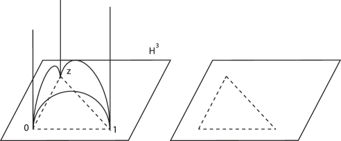
Figure 25: An ideal tetrahedron in $\mathbb{H}^{3}$ has all four vertices on the boundary of $\mathbb{H}^{3}$, which we can take to be $\{0,1,z,\infty\}\in\mathbb{C}\cup\{\infty\}$.

A tetrahedron has six edges and, correspondingly, six face angles. For an ideal tetrahedron with modulus $z$, the two face angles on the opposite side of the tetrahedron are the same. These are given as the arguments of three complex parameters

$$z\ ,\quad z^{\prime}:=\frac{1}{1-z}\ ,\quad z^{\prime\prime}:=1-z^{-1}\,,$$ (B.3)

satisfying $zz^{\prime}z^{\prime\prime}=-1$. These three distinct parametrizations of the tetrahedron modulus will play an important later, when we discuss our rules.

When we glue the tetrahedra to construct 3-manifolds, we need to ensure that the angles around an edge sum up to $2\pi$. Since the angles of tetrahedra could be described either by $z,z^{\prime}$ or $z^{\prime\prime}$ depending on the parametrization, we have

$$\prod_{m:\,{\rm type\ 1}}z^{(m)}\prod_{m:\,{\rm type\ 2}}z^{\prime(m)}\prod_{m:\,{\rm type\ 3}}z^{\prime\prime(m)}=1\ ,$$ (B.4)

where we classified a tetrahedron $m$ depending on whether the angle around the edge is parametrized by $z^{(m)},z^{\prime(m)}$ or $z^{\prime\prime(m)}$. We call these equations gluing equations. In the boundary torus this simply represents the the condition that the product of $z$ around a vertex is trivial. We refer to this equation in section 4.5.

Appendix C Dehn Twists as Flips

As explained in the main text, an element of the mapping class group could be represented as a sequence of flips on the 2d triangulation. In this appendix we identify this flip sequence systematically. This result will be important for practical computations.

The mapping class group is generated by the Dehn twist $D_{\gamma}$ along non-contractible cycles (Figure 26). Moreover explicit generators and relations for the mapping class group of $\Sigma_{g,h}$ are known in the literature (see e.g. Birman ; Gervais ). This means that all we need to do is to identify an explicit sequence of flips corresponding to a single Dehn twist.

Figure 26: A Dehn twist along a non-contractible cycle (colored red).

Suppose that we perform a Dehn twist along a non-contractible cycle $\gamma$, which intersects several triangles as in Figure 27 (a). We can then verify that the flips shown in Figure 27 (b) and (c) realize the Dehn twist. Note also we need to exchange the labels appropriately after the flips. This is a rather general rule, which applies to any triangulation and to surfaces of any genus.

Figure 27: A flip sequence for a Dehn twist along a cycle $\gamma$. (a) The cycle $\gamma$ intersects many triangles along the way, some of which have an extra edge on the left and some on the right. We have highlighted all the triangles on the left side (colored red) and some on the right (colored green). (b) For each red/green block, we perform a sequence of flips, as here. (c) By repeating (b), and effectively shifting the position of one triangle one by one, we obtain a Dehn twist on the triangulation.

The situation is especially simple in the case of the $1$-punctured torus, studied in detail in Terashima:2011qi ; Terashima:2011xe — the Dehn twist along the $\alpha,\beta$-cycles both correspond to a single flip.

For the $n$-punctured sphere, consider a cycle encircling the $i$-th and $(i+1)$-th punctures, and the corresponding Dehn twist $s_{i}$. These Dehn twists generate the braid group. We can verify that this Dehn twist $s_{i}$, in the triangulations in Figures 28 and 29, are given by either $2$ or $4$ flips.

Figure 28: A Dehn twist along the red cycle could be traded for two flips (and re-labeling).

Figure 29: The Dehn twist ($s_{i}$) on the $n$-punctured sphere could be traded for two or four flips (and re-labeling).

References

- (1) Y. Terashima and M. Yamazaki, SL(2,R) Chern-Simons, Liouville, and Gauge Theory on Duality Walls, JHEP 1108 (2011) 135, [arXiv:1103.5748].
- (2) T. Dimofte, D. Gaiotto, and S. Gukov, Gauge Theories Labelled by Three-Manifolds, arXiv:1108.4389.
- (3) S. Cecotti, C. Cordova, and C. Vafa, Braids, Walls, and Mirrors, arXiv:1110.2115.
- (4) N. Drukker, D. Gaiotto, and J. Gomis, The Virtue of Defects in 4D Gauge Theories and 2D CFTs, arXiv:1003.1112.
- (5) T. Dimofte, S. Gukov, and L. Hollands, Vortex Counting and Lagrangian 3-manifolds, arXiv:1006.0977.
- (6) K. Hosomichi, S. Lee, and J. Park, AGT on the S-duality Wall, arXiv:1009.0340.
- (7) E. Witten, QUANTIZATION OF CHERN-SIMONS GAUGE THEORY WITH COMPLEX GAUGE GROUP, Commun. Math. Phys. 137 (1991) 29–66.
- (8) E. Witten, Analytic Continuation Of Chern-Simons Theory, arXiv:1001.2933.
- (9) A. Kapustin, B. Willett, and I. Yaakov, Exact Results for Wilson Loops in Superconformal Chern- Simons Theories with Matter, JHEP 03 (2010) 089, [arXiv:0909.4559].
- (10) D. L. Jafferis, The Exact Superconformal R-Symmetry Extremizes Z, arXiv:1012.3210.
- (11) N. Hama, K. Hosomichi, and S. Lee, Notes on SUSY Gauge Theories on Three-Sphere, arXiv:1012.3512.
- (12) N. Hama, K. Hosomichi, and S. Lee, SUSY Gauge Theories on Squashed Three-Spheres, arXiv:1102.4716.
- (13) Y. Terashima and M. Yamazaki, Semiclassical Analysis of the 3d/3d Relation, arXiv:1106.3066.
- (14) K. Nagao, Y. Terashima, and M. Yamazaki, Hyperbolic 3-manifolds and Cluster Algebras, arXiv:1112.3106.
- (15) T. Dimofte and S. Gukov, Chern-Simons Theory and S-duality, arXiv:1106.4550.
- (16) T. Dimofte, D. Gaiotto, and S. Gukov, 3-Manifolds and 3d Indices, arXiv:1112.5179.
- (17) J. Teschner and G. Vartanov, 6j symbols for the modular double, quantum hyperbolic geometry, and supersymmetric gauge theories, arXiv:1202.4698.
- (18) D. Gang, E. Koh, and K. Lee, Superconformal Index with Duality Domain Wall, JHEP 1210 (2012) 187, [arXiv:1205.0069].
- (19) C. Cordova, S. Espahbodi, B. Haghighat, A. Rastogi, and C. Vafa, Tangles, Generalized Reidemeister Moves, and Three-Dimensional Mirror Symmetry, arXiv:1211.3730.
- (20) A. Kapustin and M. J. Strassler, On mirror symmetry in three-dimensional Abelian gauge theories, JHEP 9904 (1999) 021, [hep-th/9902033].
- (21) E. Witten, SL(2,Z) action on three-dimensional conformal field theories with Abelian symmetry, hep-th/0307041.
- (22) S. Cecotti, A. Neitzke, and C. Vafa, R-Twisting and 4d/2d Correspondences, arXiv:1006.3435.
- (23) V. Fock and A. Goncharov, Moduli spaces of local systems and higher Teichmüller theory, Publ. Math. Inst. Hautes Études Sci. (2006), no. 103 1–211.
- (24) W. D. Neumann and D. Zagier, Volumes of hyperbolic three-manifolds, Topology 24 (1985), no. 3 307–332.
- (25) S. Fomin and A. Zelevinsky, Cluster algebras I: Foundations, J. Amer. Math. Soc. 15 (2002), no. 2 497–529.
- (26) B. Keller, “Cluster algebras, quiver representations and triangulated categories.” arXiv:0807.1960.
- (27) D. Gaiotto, G. W. Moore, and A. Neitzke, Framed BPS States, arXiv:1006.0146.
- (28) N. Seiberg, Electric - magnetic duality in supersymmetric nonAbelian gauge theories, Nucl.Phys. B435 (1995) 129–146, [hep-th/9411149].
- (29) V. V. Fock and A. B. Goncharov, Cluster ensembles, quantization and the dilogarithm, Ann. Sci. Éc. Norm. Supér. (4) 42 (2009), no. 6 865–930.
- (30) V. V. Fock and A. B. Goncharov, The quantum dilogarithm and representations of quantum cluster varieties, Invent. Math. 175 (2009), no. 2 223–286.
- (31) M. Kontsevich and Y. Soibelman, Stability structures, motivic Donaldson-Thomas invariants and cluster transformations, arXiv:0811.2435.
- (32) R. M. Kashaev and T. Nakanishi, Classical and quantum dilogarithm identities, arXiv:1104.4630.
- (33) G. Festuccia and N. Seiberg, Rigid Supersymmetric Theories in Curved Superspace, JHEP 1106 (2011) 114, [arXiv:1105.0689].
- (34) N. A. Nekrasov and S. L. Shatashvili, Supersymmetric vacua and Bethe ansatz, Nucl.Phys.Proc.Suppl. 192-193 (2009) 91–112, [arXiv:0901.4744].
- (35) T. Dimofte, Quantum Riemann Surfaces in Chern-Simons Theory, arXiv:1102.4847.
- (36) A. Kapustin, B. Willett, and I. Yaakov, Exact results for supersymmetric abelian vortex loops in 2+1 dimensions, arXiv:1211.2861.
- (37) N. Drukker, T. Okuda, and F. Passerini, Exact results for vortex loop operators in 3d supersymmetric theories, arXiv:1211.3409.
- (38) J. J. Heckman, C. Vafa, D. Xie, and M. Yamazaki, String Theory Origin of Bipartite SCFTs, arXiv:1211.4587.
- (39) S. Cecotti and C. Vafa, Classification of complete N=2 supersymmetric theories in 4 dimensions, arXiv:1103.5832.
- (40) L. Chekhov and V. Fock, Quantum Teichmuller space, Theor.Math.Phys. 120 (1999) 1245–1259, [math/9908165].
- (41) R. M. Kashaev, Quantization of Teichmüller spaces and the quantum dilogarithm, Lett. Math. Phys. 43 (1998), no. 2 105–115.
- (42) L. Faddeev and A. Y. Volkov, Abelian current algebra and the Virasoro algebra on the lattice, Phys. Lett. B 315 (1993), no. 3-4 311–318.
- (43) L. D. Faddeev and R. M. Kashaev, Quantum dilogarithm, Modern Phys. Lett. A 9 (1994), no. 5 427–434.
- (44) L. D. Faddeev, Discrete Heisenberg-Weyl group and modular group, Lett. Math. Phys. 34 (1995), no. 3 249–254, [hep-th/9504111].
- (45) D. Gaiotto and E. Witten, Supersymmetric Boundary Conditions in N=4 Super Yang-Mills Theory, arXiv:0804.2902.
- (46) D. Gaiotto and E. Witten, S-Duality of Boundary Conditions In N=4 Super Yang-Mills Theory, arXiv:0807.3720.
- (47) D. Gaiotto, N=2 dualities, arXiv:0904.2715.
- (48) M. Gekhtman, M. Shapiro, and A. Vainshtein, Cluster algebras and Poisson geometry, vol. 167 of Mathematical Surveys and Monographs. American Mathematical Society, Providence, RI, 2010.
- (49) S. Fomin, M. Shapiro, and D. Thurston, Cluster algebras and triangulated surfaces. I. Cluster complexes, Acta Math. 201 (2008), no. 1 83–146.
- (50) V. V. Fock, Dual Teichmüller spaces, hep-th/9702018.
- (51) W. Floyd and A. Hatcher, Incompressible surfaces in punctured-torus bundles, Topology Appl. 13 (1982), no. 3 263–282.
- (52) M. Lackenby, The canonical decomposition of once-punctured torus bundles, Comment. Math. Helv. 78 (2003), no. 2 363–384.
- (53) F. Guéritaud, On canonical triangulations of once-punctured torus bundles and two-bridge link complements, Geom. Topol. 10 (2006) 1239–1284. With an appendix by David Futer.
- (54) M. Sakuma and J. Weeks, Examples of canonical decompositions of hyperbolic link complements, Japan. J. Math. (N.S.) 21 (1995), no. 2 393–439.
- (55) D. Futer and F. Gueritaud, Explicit angle structure for veering triangulations, arXiv:1012.5134.
- (56) J. S. Birman, Braids, links, and mapping class groups. Princeton University Press, Princeton, N.J., 1974. Annals of Mathematics Studies, No. 82.
- (57) K. Hikami and R. Inoue, Cluster Algebra and Complex Volume of Once-Punctured Torus Bundles and Two-Bridge Knots, arXiv:1212.6042.
- (58) W. P. Thurston, The geometry and topology of three-manifolds, 1978-79.
- (59) D. Xie and M. Yamazaki, Network and Seiberg Duality, JHEP 1209 (2012) 036, [arXiv:1207.0811].
- (60) S. Franco, Bipartite Field Theories: from D-Brane Probes to Scattering Amplitudes, arXiv:1207.0807.
- (61) A. Hashimoto, P. Ouyang, and M. Yamazaki, in progress.
- (62) N. Reshetikhin and V. G. Turaev, Invariants of -manifolds via link polynomials and quantum groups, Invent. Math. 103 (1991), no. 3 547–597.
- (63) M. Alim, S. Cecotti, C. Cordova, S. Espahbodi, A. Rastogi, et al., N=2 Quantum Field Theories and Their BPS Quivers, arXiv:1112.3984.
- (64) D. Xie, BPS spectrum, wall crossing and quantum dilogarithm identity, arXiv:1211.7071.
- (65) A. Goncharov and R. Kenyon, Dimers and cluster integrable systems, arXiv:1107.5588.
- (66) S. Franco, Dimer Models, Integrable Systems and Quantum Teichmuller Space, JHEP 1109 (2011) 057, [arXiv:1105.1777].
- (67) N. Arkani-Hamed, J. L. Bourjaily, F. Cachazo, A. B. Goncharov, A. Postnikov, et al., Scattering Amplitudes and the Positive Grassmannian, arXiv:1212.5605.
- (68) Y. Terashima and M. Yamazaki, Emergent 3-manifolds from 4d Superconformal Indices, Phys.Rev.Lett. 109 (2012) 091602, [arXiv:1203.5792].
- (69) M. Yamazaki, Quivers, YBE and 3-manifolds, JHEP 1205 (2012) 147, [arXiv:1203.5784].
- (70) L. D. Faddeev, R. M. Kashaev, and A. Y. Volkov, Strongly coupled quantum discrete Liouville theory. I: Algebraic approach and duality, Commun. Math. Phys. 219 (2001) 199–219, [hep-th/0006156].
- (71) W. P. Thurston, Three-dimensional manifolds, Kleinian groups and hyperbolic geometry, Bull. Amer. Math. Soc. (N.S.) 6 (1982), no. 3 357–381.
- (72) S. Gervais, A finite presentation of the mapping class group of a punctured surface, Topology 40 (2001), no. 4 703–725.