A continuation method for the efficient solution of parametric optimization problems in kinetic model reduction

Abstract

Model reduction methods often aim at an identification of slow invariant manifolds in the state space of dynamical systems modeled by ordinary differential equations. We present a predictor corrector method for a fast solution of an optimization problem the solution of which is supposed to approximate points on slow invariant manifolds. The corrector method is either an interior point method or a generalized Gauss–Newton method. The predictor is an Euler prediction based on the parameter sensitivities of the optimization problem. The benefit of a step size strategy in the predictor corrector scheme is shown for an example.

1 Introduction

Models including multiple time scales arise in many applications as e.g. combustion chemistry and biochemistry. The models under consideration are described by a system of ordinary differential equations (ODE). Model reduction methods for stiff multiple time scale ODE aim at an identification of the slow directions in the phase space of the system. After a short relaxation phase, the dynamics of the ODE model are mainly determined by the slow modes.

The slow dynamics are often described by so-called slow invariant manifolds (SIM). In the phase space of the dynamical system under consideration, trajectories bundle on those SIM being attractors of nearby trajectories. These are hierarchically ordered with decreasing dimension towards stable equilibrium, and the dimension corresponds to the set of slow (large) time scales. Fenichel analyzes slow manifolds in context of singular perturbed systems of ODE in a series of articles [11, 12, 13, 14]. It is shown there that for a sufficiently large separation of time scales (a sufficiently small singular perturbation parameter) there exists a mapping from a compact subset of the subspace of slow variables into the subspace of fast variables. The graph of this mapping is the slow manifold.

Many model reduction methods identify or approximate such SIM. The quasi steady state approximation identifies the slow manifold of singular perturbed systems of ODE by setting the singular perturbation parameter to zero [7, 9, 35]. The dynamics are only described by the differential algebraic equation that consists of the ODE for the slow variables and the implicit function relating the fast variables to the slow ones and defining the slow manifold. The ILDM method identifies a local SIM approximation based on an eigenvalue decomposition of the Jacobian of the right hand side of the ODE [29]. The CSP method identifies a local basis where fast and slow dynamics in the phase space are separated [23]. Many more methods for model reduction based on an analysis of a separation of time scales exist, see e.g. the review [21].

In this article, we discuss the development of an efficient application of a model reduction method based on optimization of trajectories to models including realistic detailed chemical combustion mechanisms. In Section 2, we review the optimization problem for model reduction. The numerical optimization method to solve this optimization problem is explained in Section 3. A continuation method including the optimization method as corrector is introduced in Section 4. Existence of a homotopy path is regarded as well as a step size strategy for efficient progress. In Section 5, results of an application to example problems are shown. The article is summarized in Section 6 and an outlook is given.

2 Optimization based model reduction

An approach for model reduction based on optimization of trajectories is raised in [24]. The idea is to identify certain trajectories along which a criterion takes its minimum value that represents a mathematical characterization of slowness and attraction of nearby trajectories. This relaxation criterion is minimized subject to the constraints of the dynamics, the fixed parameters for parametrization of the SIM, and eventual conservation laws.

2.1 Optimization problem

In [27], it is shown for two specific models that the method identifies asymptotically the correct SIM. Here we stick near to the formulation chosen there. We denote the ODE that describe the dynamics of the kinetic system with

$$\mathrm{D}z(t)=S(z(t)),$$ (1)

where $\mathrm{D}$ is the derivative of state vector $z(t)$ at time $t$ w.r.t. $t$. The function $S:\mathrm{D}\rightarrow\mathbb{R}^{n}$ is assumed sufficiently smooth in an open domain $D\in\mathbb{R}^{n}$. Conservation relations are valid for many models. Typically, these are restrictions to an initial value $z(t_{0})$ for an initial value problem with the dynamics (1) and represent the conservation of the mass of chemical elements in the system.

A subset of state variables is usually chosen for parametrization of the SIM approximation. In our formulation, these variables $z_{j}(t_{*})$, $j\in\mathcal{I}_{\text{pv}}$, which are called reaction progress variables or represented species, are fixed at $t_{*}$ to a certain value $z_{j}^{t_{*}},$ $j\in\mathcal{I}_{\text{pv}}$ with $|\mathcal{I}_{\text{pv}}|<n$. The aim of a model reduction method that allows for species reconstruction is the computation of the corresponding unrepresented variables $z_{j}(t_{*})$, $j\notin\mathcal{I}_{\text{pv}}$, at $t_{*}$ leading to a local representation of the SIM.

A general formulation of the optimization problem (similar to [27]) to compute an approximation of a SIM is given by

$$\min_{z}\ \Psi(z)$$ (2a)

subject to

$$\mathrm{D}z(t) =S(z(t))$$ (2b)

$$0 =\bar{C}(z(t))$$ (2c)

$$0 =z_{j}(t_{*})-z_{j}^{t_{*}},\quad j\in\mathcal{I}_{\text{pv}}$$ (2d)

$$0 \leqslant z(t)$$ (2e)

and

$$t \in[t_{0},t_{\mathrm{f}}]$$ (2f)

$$t_{*} \in[t_{0},t_{\mathrm{f}}]\quad\text{(fixed)}.$$ (2g)

This means, a trajectory (piece) $z$ has to be identified on an interval $[t_{0},t_{\mathrm{f}}]$ such that the trajectory obeys the ODE (2b) and necessary conservation relations (2c). The reaction progress variables are fixed to the desired values $z_{j}^{t_{*}}$, $j\in\mathcal{I}_{\text{pv}}$ at a point in time $t_{*}$ in the interval $[t_{0},t_{\mathrm{f}}]$ in Eq. (2d). In some applications, positivity of the state variables has to be demanded explicitly to guarantee physical feasibility in the iterative solution algorithm for problem (2) as it is done in (2e).

2.1.1 Objective function

Various suggestions for a suitable objective functional $\Psi$ have been made, especially in [25]. In [27], the objective function

$$\Psi(z)\mathrel{\mathop{:}}=\int_{t_{0}}^{t_{\textrm{f}}}\Phi\left(z(t)\right)\;\mathrm{d}t$$ (3)

with the integrand

$$\Phi(z(t))=\|J_{S}(z(t))\;S(z(t))\|_{2}^{2}$$

in the Lagrange term is used, where $J_{S}$ denotes the Jacobian of $S$.

This might be motivated by the estimate

$$\|J_{S}\;S\|_{2}\leqslant\|J_{S}\|_{2}\;\|S\|_{2},$$

where a small spectral norm $\|J_{S}\|_{2}$ relates to the attraction property of the SIM and a small $\|S\|_{2}$ relates to slowness.

2.1.2 Local formulation

The approximation of points on the SIM computed as solution of optimization problem (2) is often used e.g. in computational fluid dynamics (CFD) and other applications. In this context, a large number of approximation points of the SIM for different values of the reaction progress variables is needed. This means, problem (2) has to be solved repeatedly for a range of values of $z_{j}^{t_{*}}$, $j\in\mathcal{I}_{\text{pv}}$. This is generally very time consuming.

In this case, a local formulation (in time) can be used. It is given by (cf. [20])

$$\min_{z(t_{*}),T(t_{*})}\;\|J_{S}(z(t_{*}))\;S(z(t_{*}))\|_{2}^{2}$$ (4a)

subject to

$$0 =C(z(t_{*}))$$ (4b)

$$0 =z_{j}(t_{*})-z_{j}^{t_{*}},\quad j\in\mathcal{I}_{\text{pv}}$$ (4c)

$$0 \leqslant z(t_{*}).$$ (4d)

In the case of the objective function $\Psi$ in (3), optimization problem (2) is semi-infinite. A discretization method such as a collocation of orthogonal polynomials or a shooting approach has to be applied to project it into a finite nonlinear programming (NLP) problem. If (4) is used, the optimization problem is a finite dimensional NLP problem, and the solution of the system dynamics (2b) is dispensable. This problem can be solved directly with standard NLP software as sequential quadratic programming [31] or interior point [19] methods.

2.2 Parametric optimization

In the optimization problem which is solved for model reduction purposes, there is a parameter dependence in terms of the fixation of the reaction progress variables. Therefore, we consider parametric finite dimensional NLP problems in the following. The standard problem is given as

$$\min_{x\in\mathbb{R}^{n}}f(x,r)$$ (5a)

subject to

$$g(x,r) =0$$ (5b)

$$h(x,r) \geqslant 0,$$ (5c)

where the objective function $f:D\times\tilde{D}\rightarrow\mathbb{R}$, the equality constraint function $g:D\times\tilde{D}\rightarrow\mathbb{R}^{n_{2}}$, and the inequality constraint function $h:D\times\tilde{D}\rightarrow\mathbb{R}^{n_{3}}$ depend on the parameter vector $r\in\tilde{D}$ with both $D\subset\mathbb{R}^{n}$, $\tilde{D}\subset\mathbb{R}^{n_{r}}$ open. The Lagrangian function can be written as

$$\mathcal{L}(x,\lambda,\mu,r)\mathrel{\mathop{:}}=f(x,r)-\lambda^{\mathrm{T}}g(x,r)-\mu^{\mathrm{T}}h(x,r).$$

First order sensitivity results are given by the following theorem of Fiacco [16]. These results are used in context of real-time optimization, see e.g. [8], and nonlinear model predictive control, e.g. in [15, 40], for embedding of neighboring solutions of a function of a parameter $r$.

Theorem 1 (Second-order sufficient conditions [30]).

Let $x^{*}$ be a feasible point of (5) for which the KKT conditions are satisfied with Lagrange multipliers $(\lambda^{*},\mu^{*})$. Suppose further that

$$v^{\mathrm{T}}\nabla_{\!xx\,}^{2}\mathcal{L}(x^{*},\lambda^{*},\mu^{*},r)v>0\quad\forall v\in\mathcal{C}(x^{*},\lambda^{*},\mu^{*}),\ v\neq 0,$$

where $\mathcal{C}$ is the critical cone. Then $x^{*}$ is a strict local minimizer for (5).

Proof.

See e.g. [17, 30]. ∎

Theorem 2 (Parameter sensitivity [16]).

Let the functions $f$, $g$, and $h$ in problem (5) be twice continuously differentiable in a neighborhood of $(x^{*},0)$. Let the second order sufficient conditions hold (see Theorem 1) for a local minimum of (5) at $x^{*}$ with $r=0$ and Lagrange multipliers $\lambda^{*}$, $\mu^{*}$. Furthermore, let linear independence constraint qualification (LICQ) be valid in $(x^{*},0)$ and strict complementary slackness, i.e. $\mu_{i}^{*}>0$ if $h_{i}(x^{*},0)=0$, $i=1,\dots,n_{3}$. Then the following holds:

1. The point $x^{*}$ is a isolated local minimizer of (5) with $r=0$, and the associated Lagrange multipliers $\lambda^{*}$, $\mu^{*}$ are unique.

2. For $r$ in a neighborhood of $0$, there exists a unique once continuously differentiable function $(x(r),\lambda(r),\mu(r))$ satisfying the second order sufficient conditions for a local minimum of (5) such that

   $$(x(0),\lambda(0),\mu(0))=(x^{*},\lambda^{*},\mu^{*}),$$

   and $x(r)$ is a isolated local minimizer of (5) with Lagrange multipliers $\lambda(r)$ and $\mu(r)$.

3. Strict complementarity with respect to $\mu(r)$ and LICQ hold at $x(r)$ for $r$ near $0$.

Proof.

See [16]. ∎

Numerically, the inequality constraints (5c) can be treated with either an active set (AS) strategy or an interior point (IP) method. In an AS strategy, the AS is updated in each iteration. Active constraints are considered as equality constraints, inactive constraints are omitted. By contrast, the objective function is modified with a barrier term eliminating the inequality constraints in an IP framework. Therefore, we only regard equality constraints in the following.

The necessary optimality (KKT) conditions (stationarity of the Lagrangian function, feasibility, and complementarity) for problem (14) can shortly be written as

$$K(x,\lambda,\mu,r)=0.$$ (6)

with e.g. for an active set method

$$K(x,\lambda,\mu,r)\mathrel{\mathop{:}}=\left\{\begin{aligned} &\nabla f(x,r)-\nabla_{\!x\,}g(x,r)\lambda-\nabla_{\!x\,}h(x,r)\mu\\ &g(x,r)\\ &h_{i}(x,r),\quad i\in\mathcal{A}(x),\end{aligned}\right.$$

We are interested in the derivative of the solution $(x^{*}(r),\lambda^{*}(r),\mu^{*}(r))$ of (6) with respect to the parameters. The implicit function theorem yields

$$\mathrm{D}_{(x,\lambda,\mu)}K(x^{*},\lambda^{*},\mu^{*},r)\;\mathrm{D}_{r}(x,\lambda,\mu)=-\mathrm{D}_{r}K(x^{*},\lambda^{*},\mu^{*},r).$$

The symbol $\mathrm{D}_{x}f$ denotes the partial derivative of $f$ w.r.t. $x$. The same equation in matrix notation is

$$\begin{bmatrix}\mathrm{D}_{x}K&\mathrm{D}_{\lambda}K&\mathrm{D}_{\mu}K\end{bmatrix}\begin{bmatrix}\mathrm{D}_{r}x\\ \mathrm{D}_{r}\lambda\\ \mathrm{D}_{r}\mu\end{bmatrix}=-\mathrm{D}_{r}K.$$ (7)

The KKT matrix

$$\begin{bmatrix}\mathrm{D}_{x}K&\mathrm{D}_{\lambda}K&\mathrm{D}_{\mu}K\end{bmatrix}$$ (8)

is nonsingular if LICQ and second order sufficient optimality conditions [17, 30] are fulfilled.

3 Numerical solution of the optimization problem (4)

The optimization problem (4) is a constrained nonlinear least squares (CNLLS) problem of the form

$$\min_{x\in\mathbb{R}^{n}}\;\tfrac{1}{2}\|F_{1}(x)\|_{2}^{2}$$ (9a)

subject to

$$F_{2}(x) =0$$ (9b)

where the functions $F_{i}:D\rightarrow\mathbb{R}^{n_{i}},\ i=1,2$, are supposed to be at least twice continuously differentiable in their open domain $D\subset\mathbb{R}^{n}$. The problem is solved iteratively: $x_{k+1}=x_{k}+t_{k}d_{k}$, where $d_{k}\in\mathbb{R}^{n}$ is the increment and $t_{k}\in(0,1]$ the step length.

In order to solve this CNLLS problem, we use a generalized Gauss–Newton (GGN) method as described in [6, 37], where the step direction (increment) is computed as solution of the linearized optimization problem

$$\min_{d\in\mathbb{R}^{n}}\;\tfrac{1}{2}\|F_{1}(x_{k})+J_{1}(x_{k})d\|_{2}^{2}$$ (10a)

subject to

$$F_{2}(x_{k})+J_{2}(x_{k})d =0$$ (10b)

where $J_{i}$ is the Jacobian matrix of $F_{i}$ for $i=1,2$.

An AS strategy is used to treat inequality constraints. For globalization, we employ a filter method [18]. The filter is implemented as in [38, 39]. The most important feature of a filter is the fact, that a step is accepted if it improves the value of the objective function or the constraint violation. The combination of a GGN method with a filter method for globalization of convergence is new to our knowledge.

To prevent the Maratos effect [30], we use a second order correction (SOC) as in [38, 39]. The SOC increment is computed as solution of the least squares problem, cf. [30]:

$$\min_{\check{d}}\;\|\check{d}\|_{2}^{2}$$ (11)

subject to

$$F_{2}(x+d)+J_{2}(x)\check{d}=0.$$

If a trial point is not accepted by the filter after several reductions of the step size, a feasibility restoration phase is necessary. This can be done efficiently in context of a Gauss-Newton method. The aim of the feasibility restoration phase is the computation of a feasible point that is “near” to the last accepted iterate and acceptable to the updated filter.

The goal to find a feasible point that is “near” to the last iterate $x=x_{k}$ can be written in context of GGN methods as the following CNLLS problem

$$\min_{\bar{x}}\;\tfrac{1}{2}\|\bar{x}-x\|_{2}^{2}$$ (12a)

subject to

$$F_{2}(\bar{x}) =0$$ (12b)

Problem (12) can be solved iteratively with an increment $\bar{d}_{kl}$ with the new iteration index $l$ as solution of a CLLS optimization problem

$$\min_{\bar{d}}\;\tfrac{1}{2}\|\bar{x}_{k}-x+\bar{d}\|_{2}^{2}$$ (13a)

subject to

$$F_{2}(\bar{x}_{k})+J_{2}(\bar{x}_{k})\bar{d} =0$$ (13b)

and initial value $\bar{x}^{0}\mathrel{\mathop{:}}=x$. The only difference between (13) and problem (10) is the objective function, matrix factorizations, e.g. of $J_{2}$, can be reused.

4 Continuation strategy

It is useful to follow the homotopy path of the zero of the KKT conditions in dependence of the reaction progress variables to solve families of optimization problems alike (2) for different parameters.

In the following, we consider the finite dimensional parametric optimization problem

$$\min_{x\in\mathbb{R}^{n}}\ f(x)$$ (14a)

subject to

$$0 =g(x)$$ (14b)

$$0 =x_{j(i)}-r^{i},\quad i=1,\dots,n_{r}$$ (14c)

where the functions $f:D\rightarrow\mathbb{R}$ and $g:D\rightarrow\mathbb{R}^{n_{2}}$ are $\mathcal{C}^{2}(D)$ in the open domain $D\subset\mathbb{R}^{n}$. The fixed values of the reaction progress variables in (14c) are denoted by the parameter vector $r\in\mathbb{R}^{n_{r}}$, $r^{i}=z_{j(i)}^{t_{*}}$, $i=1,\dots,n_{r}$, $n_{r}<n-n_{2}$ with the notation of Equation (2d), where $j:\{1,\dots,n_{r}\}\rightarrow\mathcal{I}_{\text{pv}}$, $i\mapsto j(i)$ is a bijective map to the index set $\mathcal{I}_{\text{pv}}\subset\{1,\dots,n\}$ of the reaction progress variables.

4.1 Parameter sensitivities in the GGN method

If Newton’s method together with an active set method is used to find a candidate solution of (14), i.e. the computation of a root of $K$, the KKT matrix $\mathrm{D}_{(x,\lambda,\mu)}K(x_{k},\lambda_{k},\mu_{k})$ has to be computed in every iteration $k$. This is different if a generalized Gauss–Newton method is employed.

We return to the notation used in Section 3: The objective function is written as $f(x)=\|F_{1}(x)\|_{2}^{2}$ with a sufficiently smooth function $F_{1}:D\subset\mathbb{R}^{n}\rightarrow\mathbb{R}^{n_{1}}$. The constraints are given as $F_{2}:D\subset\mathbb{R}^{n}\rightarrow\mathbb{R}^{\bar{n}_{2}}$, $\bar{n}_{2}=n_{2}+n_{r}+|\mathcal{A}(x)|$ with

$$F_{2}(x)=\left\{\begin{aligned} &g(x)\\ &x_{j(i)}-r^{i},\quad i=1,\dots,n_{r}\\ &x_{i},\quad i\in\mathcal{A}(x)\end{aligned}\right.$$

and the active set $\mathcal{A}(x)$ in $x$. The Jacobian matrices of $F_{1}$ and $F_{2}$ are denoted as $J_{1}$ and $J_{2}$, respectively.

In every iteration, the equation system

$$\begin{bmatrix}J_{1}^{\mathrm{T}}J_{1}&J_{2}^{\mathrm{T}}\\ J_{2}&0\end{bmatrix}\begin{bmatrix}d\\ -\lambda\end{bmatrix}=-\begin{bmatrix}J_{1}^{\mathrm{T}}F_{1}\\ F_{2}\end{bmatrix}$$ (15)

is solved in the GGN method (where the argument $x_{k}$ is omitted and the vector $\lambda$ is used for all equality and active inequality constraints); that is the KKT system of the CLLS problem (10), see Section 3. By contrast,

$$\begin{bmatrix}\mathcal{L}_{xx}&-J_{2}^{\mathrm{T}}\\ J_{2}&0\end{bmatrix}\begin{bmatrix}\Delta x\\ \Delta\lambda\end{bmatrix}=-\begin{bmatrix}\nabla_{x}\mathcal{L}\\ F_{2}\end{bmatrix}$$ (16)

is solved if Newton’s method is applied to find a KKT point of the original CNLLS problem (9). The derivative of the Lagrangian function of the CNLLS problem is $\nabla_{\!x\,}\mathcal{L}^{\mathrm{T}}=F_{1}(x)^{\mathrm{T}}J_{1}(x)-\lambda^{\mathrm{T}}J_{2}(x)$. The difference in the KKT matrices in Equations (16) and (15) is the difference in the Hessians of the different Lagrangian functions: In the GGN method, $J_{1}^{\mathrm{T}}J_{1}$ is used; whereas Newton’s method applied to the KKT conditions of the original CNLLS problem (9) exploits

$$\mathcal{L}_{xx} =\nabla_{\!xx\,}\tfrac{1}{2}\|F_{1}(x)\|_{2}^{2}-\sum_{i=1}^{\bar{n}_{2}}\lambda_{i}\nabla_{\!xx\,}F_{2}^{i}(x)$$ (17)

$$=J_{1}^{\mathrm{T}}J_{1}+\left(\mathrm{D}_{x}J_{1}^{\mathrm{T}}\right)F_{1}-\sum_{i=1}^{\bar{n}_{2}}\lambda_{i}\nabla_{\!xx\,}F_{2}^{i}(x),$$

where $F_{2}^{i}$ is the $i$-th component of $F_{2}$.

In our application in chemical kinetics, the constraints $F_{2}$ are given via conservation relations. In this case, the second derivative $\nabla_{\!xx\,}F_{2}^{i}$ of $F_{2}^{i}$ typically is zero. This might not be true, if an entry in $F_{2}$ is a nonlinear equation in $x$ representing an energy conservation law, see also [26]. This means, the effort for computing $\mathcal{L}_{xx}$ instead of $J_{1}^{\mathrm{T}}J_{1}$ is mainly the effort to compute the expression $\left(\mathrm{D}_{x}J_{1}^{\mathrm{T}}\right)F_{1}$. This can be evaluated using automatic differentiation [22] as a directional derivative of $J_{1}$ with respect to direction $F_{1}$.

4.2 Euler predictor

If the approximation of points on the SIM is used in simulations in computational fluid dynamics, approximations of the tangent vectors of the SIM in these points are needed, too, see e.g. [34]. These are given via the parameter sensitivities $D_{r^{i}}x^{*}=\tfrac{\mathrm{d}z^{*}(t_{*})}{\mathrm{d}z_{j(i)}^{t_{*}}}$ at the solution $x^{*}$ and $z^{*}$ of the optimization problems (14) and (2), respectively. As these derivatives are available, we use the Euler prediction in a predictor corrector scheme for initialization of the optimization algorithm (corrector) to solve neighboring problems. In our case, this is the computation of a solution with the optimization algorithm for various parameter values of the reaction progress variables $r$.

The prediction can be used in a homotopy method with a step size strategy. An effective step size strategy is published in [10] and extensively discussed and modified in [3, 4, 5]. We use the method as discussed in [4]. The aim of the step length strategy of den Heijer and Rheinboldt [10] is to achieve a desired number of iterations for the corrector step. The strategy allows for the computation of a step length based on the contraction rate of the latest corrector iterations and an error model for the corrector such that the desired number of iterations is achieved.

We define a curve $c$ as a mapping from the parameter space to the space of the primal and dual variables of (14)

$$c:\mathbb{R}^{n_{r}} \rightarrow\mathbb{R}^{n+n_{2}}$$

$$r \mapsto c(r)\mathrel{\mathop{:}}=\begin{pmatrix}x^{*}(r)\\ \lambda^{*}(r)\end{pmatrix}.$$

For each value of the parameter vector $r$, $c(r)$ is the solution $(x^{*}(r),\lambda^{*}(r))$ of (14).

We denote the Euler predictor step

$$c_{i+1}^{0}(h_{i})=c_{i}+h_{i}(r_{i+1}-r_{i})^{\mathrm{T}}\tfrac{\mathrm{d}}{\mathrm{d}r}c_{i}(r_{i}),\quad i=0,\dots$$ (18)

The prediction $c_{i}^{0}$ is used as initialization of the corrector to compute the solution of (14). The corrector iterations are denoted

$$c_{i}^{j+1}(h_{i})=\mathrm{C}(c_{i}^{j}(h_{i})),\quad j=0,\dots$$

with the corrector $\mathrm{C}$. It is assumed that the corrector iterations converge to the solution

$$c_{i}^{\infty}(h_{i})\mathrel{\mathop{:}}=\lim_{j\rightarrow\infty}c_{i}^{j}(h_{i})\in K^{-1}(0).$$

The sophisticated aspect in the work of den Heijer and Rheinboldt [10] is the error model $\phi$. This error model estimates the error of the iterates

$$\epsilon_{j}(h_{i})=\|c_{i}^{\infty}(h_{i})-c_{i}^{j}(h_{i})\|_{2}$$

independently of $h$ via an expression of the form

$$\epsilon_{j+1}(h_{i})\leqslant\phi(\epsilon_{j}(h_{i})).$$

The formula for the error model depends on the contraction rate of the corrector, see [4, p. 53ff.], where we use the error model for the quadratically convergent Newton’s method and for the linearly convergent GGN method.

Linear step

Optimization problem (14) has to be solved many times for different values of the parameter $r$. Especially if the approximation of points on a SIM is needed in situ, e.g. in a CFD simulation, it is necessary to compute the solution of neighboring optimization problems fast.

If the values $r^{\textrm{new}}$ for the reaction progress variables, for which a SIM approximation is needed, are near to the values $r^{*}$

$$\|r^{\textrm{new}}-r^{*}\|_{2}<\epsilon_{\mathrm{tol}}$$ (19)

for which the optimization problem is already solved, it can save computing time to use $z^{\mathrm{lin}}$ as approximation of the SIM. This is defined (in analogy to (18)) as

$$z^{\mathrm{lin}}\mathrel{\mathop{:}}=z^{*}(t_{*})+\left(r^{\textrm{new}}-r^{*}\right)^{\mathrm{T}}\frac{\mathrm{d}z^{*}(t_{*})}{\mathrm{d}r}(r^{*})$$ (20)

where the notation is in accordance with the notation in (2), $r^{i}=z_{j(i)}^{t_{*}}$, $i=1,\dots,n_{r}$, $n_{r}=|\mathcal{I}_{\text{pv}}|$, $j$ is the bijection, and $r^{i}$ is the $i$-th component of $r$.

5 Numerical results

For numerical validation of our method, we use a test model for model reduction purposes. The reaction mechanism is given in Table 1. We use thermodynamical data in form of coefficients of NASA polynomials we received from J. M. Powers and A. N. Al-Khateeb, which they use in [1, 2].

The mechanism is published originally in [28]. The simplified version shown in Table 1 is used by Ren et al. in [33]. The mechanism consists of five reactive species and inert nitrogen, where in comparison to a full hydrogen combustion mechanism the species $\mathrm{O}_{2}$, $\mathrm{HO}_{2}$, and $\mathrm{H}_{2}\mathrm{O}_{2}$ are removed. The species are involved in six Arrhenius type reactions, where three combination/decomposition reactions require a third body for an effective collision.

Table 1: Simplified mechanism as used in [33]. Collision efficiencies $\mathrm{M}$: $\alpha_{\mathrm{H}}=1.0,\alpha_{\mathrm{H_{2}}}=2.5,\alpha_{\mathrm{OH}}=1.0$, $\alpha_{\mathrm{O}}=1.0,\alpha_{\mathrm{H_{2}O}}=12.0,\alpha_{\mathrm{N_{2}}}=1.0$; [33].

Reaction			$A$ / ($\textrm{cm},\textrm{mol},\textrm{s}$)	$b$	$E_{\textrm{a}}$ / $\mathrm{kJ}\text{\,}{\mathrm{mol}}^{-1}$
$\mathrm{O}+\mathrm{H_{2}}$	$\rightleftharpoons$	$\mathrm{H}+\mathrm{OH}$	$5.08\times 10^{04}$	$2.7$	$26.317$
$\mathrm{H_{2}}+\mathrm{OH}$	$\rightleftharpoons$	$\mathrm{H_{2}O}+\mathrm{H}$	$2.16\times 10^{08}$	$1.5$	$14.351$
$\mathrm{O}$ + $\mathrm{H_{2}O}$	$\rightleftharpoons$	$\mathrm{2}\,\mathrm{OH}$	$2.97\times 10^{06}$	$2.0$	$56.066$
$\mathrm{H_{2}}+\mathrm{M}$	$\rightleftharpoons$	$\mathrm{2}\,\mathrm{H}+\mathrm{M}$	$4.58\times 10^{19}$	$-1.4$	$436.726$
$\mathrm{O}+\mathrm{H}+\mathrm{M}$	$\rightleftharpoons$	$\mathrm{OH}+\mathrm{M}$	$4.71\times 10^{18}$	$-1.0$	$0.000$
$\mathrm{H}+\mathrm{OH}+\mathrm{M}$	$\rightleftharpoons$	$\mathrm{H_{2}O}+\mathrm{M}$	$3.80\times 10^{22}$	$-2.0$	$0.000$

The reaction system is considered under isothermal and isobaric conditions at a temperature of $T=$3000\text{\,}\mathrm{K}$$ and a pressure of $p=$101\,325\text{\,}\mathrm{Pa}$$. Hence, the state of the system is sufficiently described by the specific moles of the chemical species $z_{i}$, $i=1,\dots,n_{\textrm{spec}}$ in $\mathrm{mol}\text{\,}{\mathrm{kg}}^{-1}$.

Conservation relations for the elemental mass in this model are given in terms of amount of substance as [33]

$$n_{\mathrm{H}}+2\,n_{\mathrm{H}_{2}}+n_{\mathrm{OH}}+2\,n_{\mathrm{H}_{2}\mathrm{O}} =$1.25\text{\times}{10}^{-3}\text{\,}\mathrm{mol}$$$ (21)

$$n_{\mathrm{OH}}+n_{\mathrm{O}}+n_{\mathrm{H}_{2}\mathrm{O}} =$4.15\text{\times}{10}^{-4}\text{\,}\mathrm{mol}$$$

$$2\,n_{\mathrm{N}_{2}} =$6.64\text{\times}{10}^{-3}\text{\,}\mathrm{mol}$.$$

The total mass in the system can be computed with the values in Equation (21) and has a value of $m=$1.01\text{\times}{10}^{-4}\text{\,}\mathrm{kg}$$.

5.1 One-dimensional SIM approximation

Results of an approximation of a one-dimensional SIM are shown in Figure 1 and 2. We use $z_{\mathrm{H_{2}O}}$ as reaction progress variable and vary its value. The values of all remaining species at the solution of the different optimization problems are plotted versus $z_{\mathrm{H_{2}O}}$ in form of trajectories through the solution points $z^{*}(t_{*})$ which are shown as x marks. The computation is done with the GGN method as described in Section 3.

We use values near the equilibrium state as initial values in the optimization algorithm as we assume this point near a slow manifold. We set the values of the reaction progress variable near its initial value; see Table 2. This allows for a fast computation of a solution of the first optimization problem with $z_{\mathrm{H}_{2}\mathrm{O}}^{t_{*}}=$3\text{\,}\mathrm{mol}\text{\,}{\mathrm{kg}}^{-1}$$.

Table 2: Initial value (unscaled) for the algorithm and a solution of the optimization problem (2) as solved for the results depicted in Figure 1 to reduce the simplified hydrogen combustion model with $z_{\mathrm{H}_{2}\mathrm{O}}^{t_{*}}=$3\text{\,}\mathrm{mol}\text{\,}{\mathrm{kg}}^{-1}$$.

Variable	Initial value $z^{0}(t_{*})$	Numerical solution $z^{*}(t_{*})$
$z_{\mathrm{O}}$	$0.345\,464\,41\text{\,}$	$0.345\,637\,63\text{\,}$
$z_{\mathrm{H}_{2}}$	$2.027\,973\,2\text{\,}$	$2.028\,161\,5\text{\,}$
$z_{\mathrm{H}}$	$1.519\,563\,9\text{\,}$	$1.519\,360\,6\text{\,}$
$z_{\mathrm{OH}}$	$0.764\,549\,59\text{\,}$	$0.764\,376\,37\text{\,}$
$z_{\mathrm{H}_{2}\mathrm{O}}$	$3.000\,000\,0\text{\,}$	$3.000\,000\,0\text{\,}$
$z_{\mathrm{N}_{2}}$	$32.905\,130\text{\,}$	$32.905\,130\text{\,}$

All computations are done on an Intel^® Core${}^{\textrm{TM}}$ i5-2410M CPU with 2.30 GHz, operating system openSUSE 12.2 (x86_64) including the Linux kernel 3.4.11 and GCC 4.7.1. We do not use a step size strategy in the predictor corrector scheme. To compute the 17 points shown in Figure 1, 74 iterations are necessary, which take in sum $0.02\text{\,}\mathrm{s}$.

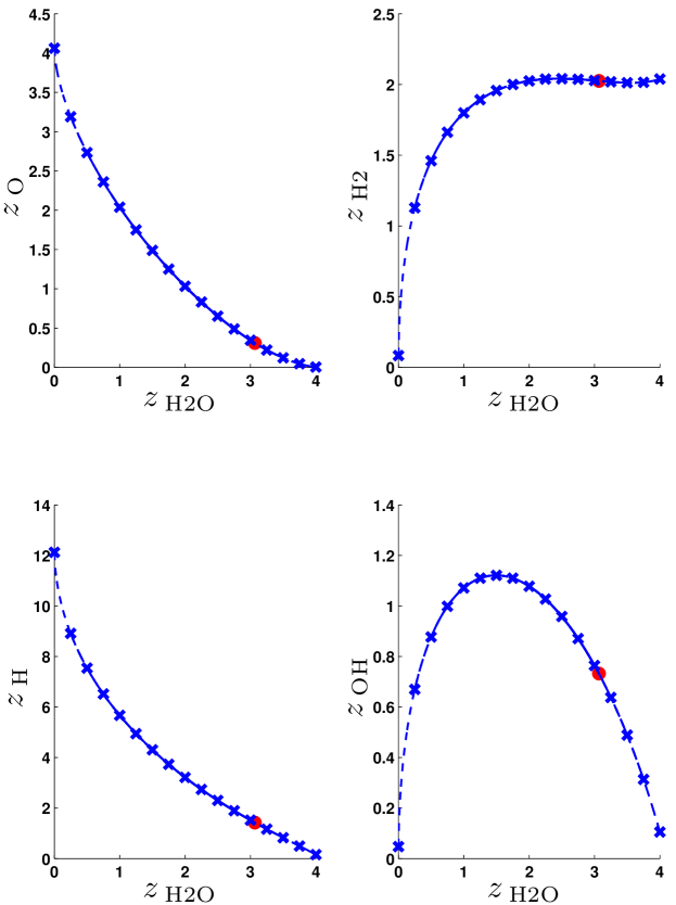
Fig. 1: Numerical solutions of the optimization problem (4) to approximate a one-dimensional manifold in the state space of the six species model for hydrogen combustion. The full dot represents the equilibrium. The x marks depict solutions $z^{*}(t_{*})$ of (4) for different values of the reaction progress variables $z_{\mathrm{H_{2}O}}$ at $t_{*}$. Trajectories through these points (curves in the figures) are also shown.

Figure 2 is presented to illustrate the linear step approximation. For the computation of the three solutions (as $\epsilon_{\mathrm{tol}}=1.1$ is chosen) of the optimization problem with different values for $z_{\mathrm{H_{2}O}}$, 15 iterations are needed (in sum), which is slightly more effort per optimization problem than in the case, where the results are illustrated in Figure 1, where the distance between the different values for $z_{\mathrm{H_{2}O}}^{t_{*}}$ is only $0.25$. It can be seen that the result of the linear approximation can lead to large deviations from a smooth, invariant manifold.

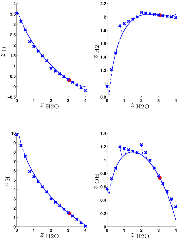
Fig. 2: Illustration of solutions of the same problem as solved for the results shown in Figure 1, but with a linear step tolerance of $\epsilon_{\mathrm{tol}}=1.1$, see (19).

Warm start with step size strategy

We want to demonstrate that a step size strategy for the warm start of the algorithm to solve neighboring optimization problems can have a benefit. So we consider the optimization problem (2) with $t_{*}=t_{\mathrm{f}}$, $t_{\mathrm{f}}-t_{0}=${10}^{-7}\text{\,}\mathrm{s}$$ to be solved for the nominal parameter $z_{\mathrm{H}_{2}\mathrm{O}}^{t_{*}}=$3\text{\,}\mathrm{mol}\text{\,}{\mathrm{kg}}^{-1}$$ with the shooting approach and Ipopt [39]. As neighboring problem we consider the parameter $z_{\mathrm{H}_{2}\mathrm{O}}^{t_{*}}=$0.5\text{\,}\mathrm{mol}\text{\,}{\mathrm{kg}}^{-1}$$. Such a large change in the parameter can occur e.g. if the presented method for model reduction is used in situ in a CFD simulation and grid refinements are performed in different regions of the spatial domain.

We solve the optimization problem first with $z_{\mathrm{H}_{2}\mathrm{O}}^{t_{*}}=$3\text{\,}\mathrm{mol}\text{\,}{\mathrm{kg}}^{-1}$$ and second with $z_{\mathrm{H}_{2}\mathrm{O}}^{t_{*}}=$0.5\text{\,}\mathrm{mol}\text{\,}{\mathrm{kg}}^{-1}$$ with a full step method in the predictor corrector scheme and apply the Euler prediction.

The computations are done on an Intel^® Core${}^{\textrm{TM}}$ i5-2410M CPU with 2.30 GHz, operating system openSUSE 12.2 (x86_64) including the Linux kernel 3.4.11 and GCC 4.7.1. Six iterations in Ipopt [39] have to be preformed to solve the nominal optimization problem and nine iterations to solve the second optimization problem. In sum, 15 iterations are necessary which take $0.82\text{\,}\mathrm{s}$ in sum.

If we initialize the step size strategy, see Section 4.2, with initial step size $h_{\textrm{init}}=\tfrac{1}{2.5}$ and the desired number of iterations $\tilde{k}=10$, we need one intermediate step in the predictor corrector scheme described in Section 4.2. This is to solve the optimization problem with the parameter $z_{\mathrm{H}_{2}\mathrm{O}}^{t_{*}}=$2\text{\,}\mathrm{mol}\text{\,}{\mathrm{kg}}^{-1}$$. In this case we need in sum $6+5+8=19$ iterations that take only $0.70\text{\,}\mathrm{s}$. The difference in the computation time arises as the point for initialization of the algorithm to solve the second optimization problem in the full step method is not near the solution such that the KKT matrix is ill-conditioned. The inertia correction in Ipopt, see [39], is activated, and 19 line search iterations are performed in sum. In case of an activated step size strategy, the initial value for the algorithm to solve the optimization problem in case of a warm start is near the solution of the optimization problem such that no inertia correction and also 19 line search iterations (one per Newton iteration) are necessary in the presented example.

For an efficient tracking of the SIM for different values of the reaction progress variables, it is important to stay close to the solution in neighboring optimization problems. Therefore, a step size strategy is beneficial.

5.2 Two-dimensional SIM approximation

We choose $z_{1}=z_{\mathrm{H}_{2}}$ and $z_{2}=z_{\mathrm{O}}$ as reaction progress variables. Numerical solutions of (2) for the reduction of the simplified model for hydrogen combustion are shown in Figure 3.

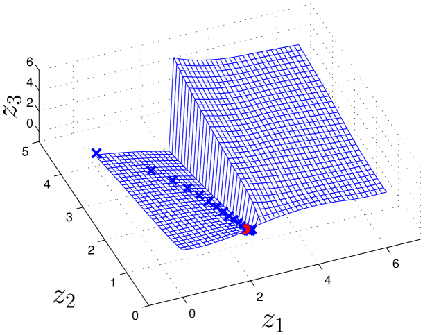
Fig. 3: Visualization of numerical solutions of the optimization problem (2) with $t_{*}=t_{\mathrm{f}}$, $t_{\mathrm{f}}-t_{0}=${10}^{-7}\text{\,}\mathrm{s}$$ to reduce the simplified hydrogen combustion model with the reaction progress variables $z_{1}$ and $z_{2}$. The solution points $z^{*}(t_{*})$ with $z_{3}=z_{\mathrm{H}_{2}\mathrm{O}}$ for different values of $(z_{1}^{t_{*}},z_{2}^{t_{*}})$ are shown as a mesh. The results shown in Figure 1 are again plotted as x marks as well as the equilibrium is shown as full dot.

Local solutions of the optimization problem (2) approximate different two-dimensional SIM for different values of the reaction progress variables. The two two-dimensional SIM come close to each other. Such occurrences can lead to severe numerical problems in the optimization algorithms as well as in the continuation algorithms as there are regions where the KKT matrix might be singular at least in the range of machine precision.

5.2.1 Optimization landscapes

We want to further illustrate this situation via optimization landscapes, i.e. graphical representations of the objective function versus the (free) optimization variables.

One reaction progress variable

In Figure 4, the value of (the objective function of the optimization problem (4)) $\Phi=\|J_{S}(z)\;S(z)\|_{2}^{2}$ is plotted versus the two degrees of freedom in (4) represented by $z_{1}$ and $z_{2}$ for one exemplary value of the one reaction progress variable $z_{3}^{t_{*}}=z_{\mathrm{H}_{2}\mathrm{O}}^{t_{*}}=$1\text{\,}\mathrm{mol}\text{\,}{\mathrm{kg}}^{-1}$$ for the simplified hydrogen combustion model.

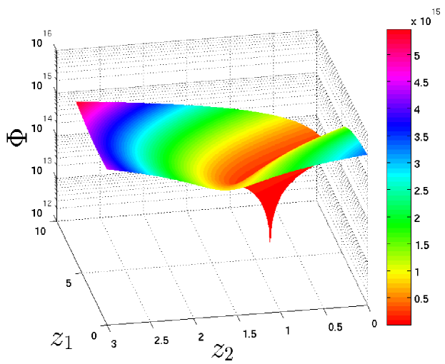
Fig. 4: Visualization of $\Phi=\|J_{S}(z)\;S(z)\|_{2}^{2}$ in dependence of $z_{1}$ and $z_{2}$ to illustrate the solution of the optimization problem (4) with $z_{3}^{t_{*}}=z_{\mathrm{H}_{2}\mathrm{O}}^{t_{*}}=$1\text{\,}\mathrm{mol}\text{\,}{\mathrm{kg}}^{-1}$$ for the reduction of the simplified hydrogen combustion model.

The $\Phi$-axis has logarithmic scale. A single local solution of the optimization problem (4) for the reduction of the simplified hydrogen combustion model can be seen.

Two reaction progress variables

To compute an optimization landscape in case of two reaction progress variables, we fix $z_{2}^{t_{*}}=z_{\mathrm{O}}^{t_{*}}=$0.3\text{\,}\mathrm{mol}\text{\,}{\mathrm{kg}}^{-1}$$. We regard the value of $\Phi=\|J_{S}(z)\;S(z)\|_{2}^{2}$ (the objective function of the optimization problem (4)) in dependence of $z_{3}$ for fixed $z_{1}$.

The results are shown in Figure 5. It can be seen that there are two distinct local minima of $\Phi=\|J_{S}(z)\;S(z)\|_{2}^{2}$ for a fixed value of e.g. $z_{1}=$2\text{\,}\mathrm{mol}\text{\,}{\mathrm{kg}}^{-1}$$: There is no unique local solution of the optimization problem (4) for the reduction of the simplified hydrogen combustion model with the reaction progress variables $z_{2}^{t_{*}}=z_{\mathrm{O}}^{t_{*}}=$0.3\text{\,}\mathrm{mol}\text{\,}{\mathrm{kg}}^{-1}$$ and $z_{1}^{t_{*}}=z_{\mathrm{H}_{2}}^{t_{*}}=$2\text{\,}\mathrm{mol}\text{\,}{\mathrm{kg}}^{-1}$$. One solution is near the value $z_{3}^{\prime}=z_{\mathrm{H}_{2}\mathrm{O}}^{\prime}=$3.1020\text{\,}\mathrm{mol}\text{\,}{\mathrm{kg}}^{-1}$$ and the other one near $z_{3}^{\prime\prime}=$5.2977\text{\,}\mathrm{mol}\text{\,}{\mathrm{kg}}^{-1}$$.

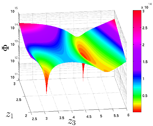
Fig. 5: Visualization of $\Phi=\|J_{S}(z)\;S(z)\|_{2}^{2}$ for the simplified hydrogen combustion model in dependence of $z_{1}$ and $z_{3}$ for a fixed value of $z_{2}=$0.3\text{\,}\mathrm{mol}\text{\,}{\mathrm{kg}}^{-1}$$. The scale for $\Phi$ is logarithmic. Consider the value of $\Phi$ in dependence of $z_{3}$ for a fixed value of $z_{1}$, e.g. for $z_{1}=$2\text{\,}\mathrm{mol}\text{\,}{\mathrm{kg}}^{-1}$$.

In this case the predictor corrector scheme helps to follow the desired local optimal solution in dependence of the reaction progress variables and not to switch to another curve $c$ of local solutions. This is only possible as long as the KKT matrix is not “too ill-conditioned”.

5.2.2 Performance test

We use the specific moles of $\mathrm{H_{2}O}$ and $\mathrm{H_{2}}$ for the parametrization of a two-dimensional SIM approximation in a performance test.

We consider a test situation of a two-dimensional grid of 108 points $(z_{\mathrm{H_{2}O}}^{t_{*}}$, $z_{\mathrm{H_{2}}}^{t_{*}})\in[0.001,0.5,1,1.5,\dots,5,5.5]\times[0.001,0.5,1,\dots,3.5,4]$, where points which violate mass conservation in combination with the positivity constraints are ignored such that 80 points remain.

Solutions of the optimization problem (4) computed with the GGN method with Euler prediction for initialization of the algorithm to solve neighboring problems are shown in Figure 6 for illustration.

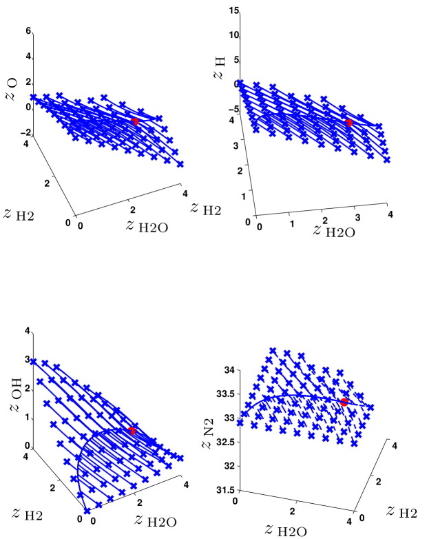
Fig. 6: Illustration of an approximation of a two-dimensional SIM in the phase space of the simplified model for hydrogen combustion. The optimization problem (4) is solved with the GGN method. The absolute tolerance for all $d_{i}$ is ${10}^{-10}\text{\,}$. The relative tolerance is ${10}^{-9}\text{\,}$. The values of the optimization variables at the solution are plotted versus the given values of the reaction progress variables shown as x marks. The trajectories started with the solution $z^{*}(t_{*})$ as initial values converge toward the equilibrium shown as full dot.

In Table 3, we compare the performance of the algorithm using the different implemented solution methods. We use the generalized Gauss–Newton method as described in Section 3 for the solution of (4). We solve the same problem with the interior point algorithm Ipopt [39]. Third, we apply a shooting approach for the semi-infinite optimization problem (2) with $t_{*}=t_{\mathrm{f}}$. The NLP problem (after solving the ODE with the BDF integrator developed by D. Skanda in [36]) is solved with Ipopt [39]. As a fourth alternative, we use a simple Gauss–Radau collocation with linear polynomials (backward Euler) for (2) with $t_{*}=t_{\mathrm{f}}$. The resulting high-dimensional NLP problem is also solved with Ipopt [39] in the latter case. For the optimization problem (2), an integration horizon of $t_{\mathrm{f}}-t_{0}=${10}^{-8}\text{\,}\mathrm{s}$$ is used.

Table 3: Comparison of the performance of the various algorithms for the reduction of the simplified model for hydrogen combustion with two reaction progress variables and full step predictor corrector method for the initialization of neighboring problems.

Method	Prediction	# Iter. w/o fail	Time	Fail	Time w/o fail
GGN	Constant	806	$0.43\text{\,}\mathrm{s}$	11	$0.18\text{\,}\mathrm{s}$
	Euler	731	$0.35\text{\,}\mathrm{s}$	11	$0.17\text{\,}\mathrm{s}$
IP for (4)	Constant	670	$1.09\text{\,}\mathrm{s}$	0	$1.09\text{\,}\mathrm{s}$
	Euler	591	$0.85\text{\,}\mathrm{s}$	0	$0.85\text{\,}\mathrm{s}$
Shooting	Constant	335	$44.15\text{\,}\mathrm{s}$	0	$44.15\text{\,}\mathrm{s}$
	Euler	258	$39.36\text{\,}\mathrm{s}$	0	$39.36\text{\,}\mathrm{s}$
Collocation	Constant	315	$95.61\text{\,}\mathrm{s}$	0	$95.61\text{\,}\mathrm{s}$
	Euler	234	$51.13\text{\,}\mathrm{s}$	0	$51.13\text{\,}\mathrm{s}$

An initialization of neighboring problems is done without step size control, as we evaluate the benefit of the Euler prediction here. The computations are done with the same computer configuration as in the example for a warm start with step size control in Section 5.1.

It can be seen that the gain in the computation time achieved by the Euler prediction in case of the collocation method, where we use 100 collocation points, is the largest with about 46.5%. This is reasonable because of the strong dependence of the collocation method on the initialization on all collocation points in the time interval $[t_{0},t_{\mathrm{f}}]$.

The benefit of the Euler prediction is about 10.8% if the shooting approach is used to solve (2). In case of the GGN method, the benefit is only 5.6% if we do not regard failures. The eleven failures only occur in the region, where $z_{\mathrm{H_{2}O}}^{t_{*}}$ is larger than the equilibrium value $z_{\mathrm{H_{2}O}}^{\textrm{eq}}$. These can not be overcome neither with the step size control for the continuation method nor with a larger tolerance for convergence in the GGN method. It can be seen that the algorithm for the solution of (4) with the GGN method is much faster than the algorithm for the solution of (2). The computation of one approximation of a point on the SIM (without regarding failures) takes about $$0.17\text{\,}\mathrm{s}$/(80-11)\approx$2.5\text{\,}\mathrm{ms}$$. This is pretty fast and might be used in an online (in situ) SIM computation during CFD simulations.

6 Conclusion

In this article, we present a strategy for an efficient solution of parametric optimization problems that arise for a method for model reduction that is raised in [24, 25, 32].

Two methods are tested to solve the semi-infinite optimization problem (2) for model reduction: collocation and shooting approaches. The resulting nonlinear programming problem is solved with a state-of-the-art open source interior point algorithm [39]. It turns out that all variants for the solution of the semi-infinite optimization problem are too slow for an in situ application of the model reduction method in e.g. a computational fluid dynamics simulation.

A finite optimization problem in form of a constrained nonlinear least squares problem can be formulated instead. This can be solved efficiently with a generalized Gauss–Newton method. A filter approach is used for globalization of convergence. Second order correction iterations prevent the Maratos effect. The problem that has to be solved in the feasibility restoration phase of the filter algorithm can also be formulated as a least squares problem such that matrix factorizations can be reused.

Parameter sensitivities of the optimization problem are used in a homotopy method for the solution of neighboring problems. The reaction progress variables for parametrization of the slow manifold are considered as parameters in the optimization problem. The problem has to be solved several times for different values of the parameters. An Euler prediction of the solution of neighboring problems is employed based on the parameter sensitivities, which are computed to obtain an approximation of the tangent space of the slow manifold. This linear prediction can be used directly within a certain tolerance as an approximation of a point on the slow manifold. It can also be used in combination with a step size strategy. The step size is computed according to [10] in dependence of the contraction of the corrector method – the solution method for the nonlinear programming problem – and the iterations needed to solve a previous optimization problem.

We study the presented methods for a simplified model for hydrogen combustion. We find that a solution of the optimization problem for approximation of points on a slow manifold can be computed in short time for the presented example. Furthermore it can be seen that there might exist several distinct local solutions of the optimization problem. In such cases, the predictor corrector scheme helps to follow one local minimum in dependence of the chosen parametrization of the slow manifold.

Such a solution strategy could also be used for variations in the model parameters as e.g. the mixture fraction, the internal energy, and others.

References

- [1] A.N. Al-Khateeb, Fine Scale Phenomena in Reacting Systems: Identification and Analysis for their Reduction, PhD thesis, University of Notre Dame, Notre Dame, Indiana, USA, 2010.
- [2] A.N. Al-Khateeb, J.M. Powers, S. Paolucci, A.J. Sommese, J.A. Diller, J.D. Hauenstein, and J.D. Mengers, One-dimensional slow invariant manifolds for spatially homogenous reactive systems, Journal of Chemical Physics, 131 (2009), p. 024118.
- [3] E. Allgower and K. Georg, Simplicial and continuation methods for approximating fixed points and solutions to systems of equations, SIAM Review, 22 (1980), pp. 28–85.
- [4] E.L. Allgower and K. Georg, Numerical Continuation Methods: An Introduction, no. 13 in Series in Computational Mathematics, Springer Verlag, Berlin, 1990.
- [5] , Numerical path following, in Techniques of Scientific Computing (Part 2), P. G. Ciarlet and J. L. Lions, eds., vol. 5 of Handbook of Numerical Analysis, Elsevier, 1997, pp. 3–207.
- [6] H.G. Bock, Randwertproblemmethoden zur Parameteridentifizierung in Systemen nichtlinearer Differentialgleichungen, in Bonner Mathematische Schriften, vol. 183, University of Bonn, 1987.
- [7] M. Bodenstein, Geschwindigkeit der Bildung des Bromwasserstoffs aus seinen Elementen, Zeitschrift für Physikalische Chemie – Leipzig, 57 (1907), pp. 168–192.
- [8] C. Büskens and H. Maurer, Sensitivity analysis and real-time optimization of parametric nonlinear programming problems, in Online Optimization of Large Scale Systems, M. Grötschel, S. O. Krumke, and J. Rambau, eds., Springer Verlag, Berlin, 2001, ch. 1, pp. 3–16.
- [9] D.L. Chapman and L.K. Underhill, The interaction of chlorine and hydrogen. The influence of mass., Journal of the Chemical Society, Transactions, 103 (1913), pp. 496–508.
- [10] C. den Heijer and W.C. Rheinboldt, On steplength algorithms for a class of continuation methods, SIAM Journal on Numerical Analysis, 18 (1981), pp. 925–948.
- [11] N. Fenichel, Persistence and smoothness of invariant manifolds for flows, Indiana University Mathematics Journal, 21 (1972), pp. 193–226.
- [12] , Asymptotic stability with rate conditions, Indiana University Mathematics Journal, 23 (1974), pp. 1109–1137.
- [13] , Asymptotic stability with rate conditions ii, Indiana University Mathematics Journal, 26 (1977), pp. 81–93.
- [14] , Geometric singular perturbation theory for ordinary differential equations, Journal of Differential Equations, 31 (1979), pp. 53–98.
- [15] H.J. Ferreau, H.G. Bock, and M. Diehl, An online active set strategy to overcome the limitations of explicit MPC, International Journal of Robust and Nonlinear Control, 18 (2008), pp. 816–830.
- [16] A.V. Fiacco, Sensitivity analysis for nonlinear programming using penalty methods, Mathematical Programming, 10 (1976), pp. 287–311.
- [17] R. Fletcher, Practical methods of optimization, vol. 2, Wiley, Chichester, 1981.
- [18] R. Fletcher and S. Leyffer, Nonlinear programming without a penalty function, Mathematical Programming, 91 (2002), pp. 239–269.
- [19] A. Forsgren, P.E. Gill, and M.H. Wright, Interior methods for nonlinear optimization, SIAM Review, 44 (2002), pp. 525–597.
- [20] S.S. Girimaji, Reduction of large dynamical systems by minimization of evolution rate, Physical Review Letters, 82 (1999), pp. 2282–2285.
- [21] A.N. Gorban, I.V. Karlin, and A.Yu. Zinovyev, Constructive methods of invariant manifolds for kinetic problems, Physics Reports, 396 (2004), pp. 197–403.
- [22] A. Griewank, Evaluating Derivatives: Principles and Techniques of Algorithmic Differentiation, no. 19 in Frontiers in Appl. Math., SIAM, Philadelphia, PA, 2000.
- [23] S.H. Lam and D.A. Goussis, The CSP method for simplifying kinetics, International Journal of Chemical Kinetics, 26 (1994), pp. 461–486.
- [24] D. Lebiedz, Computing minimal entropy production trajectories: An approach to model reduction in chemical kinetics, Journal of Chemical Physics, 120 (2004), pp. 6890–6897.
- [25] D. Lebiedz, V. Reinhardt, and J. Siehr, Minimal curvature trajectories: Riemannian geometry concepts for slow manifold computation in chemical kinetics, Journal of Computational Physics, 229 (2010), pp. 6512–6533.
- [26] D. Lebiedz and J. Siehr, Simplified reaction models for combustion in gas turbine combustion chambers, in Flow and Combustion in Advanced Gas Turbine Combustors, Amsini Sadiki, Johannes Janicka, Michael Schäfer, and Christof Heeger, eds., vol. 102 of Fluid Mechanics and its Applications, Springer, Dordrecht, 2013, ch. 5, pp. 161–182.
- [27] D. Lebiedz, J. Siehr, and J. Unger, A variational principle for computing slow invariant manifolds in dissipative dynamical systems, SIAM Journal on Scientific Computing, 33 (2011), pp. 703–720.
- [28] J. Li, Z. Zhao, A. Kazakov, and F.L. Dryer, An updated comprehensive kinetic model of hydrogen combustion, International Journal of Chemical Kinetics, 36 (2004), pp. 566–575.
- [29] U. Maas and S.B. Pope, Simplifying chemical kinetics: Intrinsic low-dimensional manifolds in composition space, Combustion and Flame, 88 (1992), pp. 239–264.
- [30] J. Nocedal and S.J. Wright, Numerical Optimization, Springer Series in Operations Research and Financial Engineering, Springer, New York, second ed., 2006.
- [31] M.J.D. Powell, A fast algorithm for nonlinearly constrained optimization calculations, in Numerical Analysis, A. Dold and B. Eckmann, eds., vol. 630 of Lecture Notes in Mathematics, Springer-Verlag Berlin, 1978, pp. 144–157.
- [32] V. Reinhardt, M. Winckler, and D. Lebiedz, Approximation of slow attracting manifolds in chemical kinetics by trajectory-based optimization approaches, Journal of Physical Chemistry A, 112 (2008), pp. 1712–1718.
- [33] Z. Ren, S.B. Pope, A. Vladimirsky, and J.M. Guckenheimer, The invariant constrained equilibrium edge preimage curve method for the dimension reduction of chemical kinetics, Journal of Chemical Physics, 124 (2006), p. 114111.
- [34] Z. Ren, S.B. Pope, A. Vladimirsky, and J.M. Guckenheimer, Application of the ICE-PIC method for the dimension reduction of chemical kinetics coupled with transport, Proceedings of the Combustion Institute, 31 (2007), pp. 473–481.
- [35] L.A. Segel and M. Slemrod, The quasi-steady-state assumption: A case study in perturbation, SIAM Review, 31 (1989), pp. 446–477.
- [36] D. Skanda, Robust optimal experimental design for model discrimination of kinetic ODE systems, PhD thesis, University of Freiburg, Freiburg im Breisgau, Germany, 2012.
- [37] J. Stoer, On the numerical solution of constrained least-squares problems, SIAM Journal on Numerical Analysis, 8 (1971), pp. 382–411.
- [38] A. Wächter and L.T. Biegler, Line search filter methods for nonlinear programming: Motivation and global convergence, SIAM Journal on Optimization, 16 (2005), pp. 1–31.
- [39] , On the implementation of a primal-dual interior point filter line search algorithm for large-scale nonlinear programming, Mathematical Programming, 106 (2006), pp. 25–57.
- [40] V.M. Zavala and L.T. Biegler, The advanced-step nmpc controller: Optimality, stability and robustness, Automatica, 45 (2009), pp. 86–93.