KCL-mth-13-01

IPMU12-0235

On Singular Fibres in F-Theory

Andreas P. Braun¹ and Taizan Watari²

¹Department of Mathematics, King‘s College, London WC2R 2LS, UK

²Institute for the Physics and Mathematics of the Universe, University of Tokyo, Kashiwano-ha 5-1-5, 277-8583, Japan

1 Introduction

Relatively to the world-sheet based formulations of string theories, Type I, Type IIA, IIB, and the Heterotic string theories, the microscopic formulation (i.e. the theoretical foundation) is less understood in 11-dimensional supergravity and F-theory. In the last years, we have seen efforts of using F-theory for a better understanding of effective low-energy physics. Despite the fact that singularities in the internal geometry play an essential role and the lack of microscopic theoretical foundations in F-theory, string dualities have been used to overcome this problem. In this paper we revisit the issue of which geometries are appropriate in F-Theory. We do not take a top-down deductive approach, but rather employ more of a try-and-error experimental technique to learn about singularities in F-theory. We feel that this might teach us important lessons about an underlying fundamental description, as one of the best test arenas for the microscopic aspects of a theory of quantum gravity (such as F-theory) must be singular geometry.

Part of the data defining a compactification of F-theory is an elliptically fibred Calabi–Yau $n$-fold $X_{n}$. To be more precise, there is a projection morphism which maps $X_{n}$ to the base manifold $B_{n-1}$,

$$\pi_{X}:X_{n}\longrightarrow B_{n-1},$$ (1)

and a section $\sigma:B_{n-1}\longrightarrow X_{n}$. By definition, the fibre of a generic point in the base is a non-singular curve of genus 1. In the context of Type IIB string theory, this fibre geometry plays a role similar to a principal bundle for vector bundles; the “structure group” is ${\rm SL}(2;\mathbb{Z})$, and various fields on $B_{n-1}$ are in various representations of the structure group. Type IIB string theory specifies the ${\rm SL}(2;\mathbb{Z})$ monodromy around a divisor $\{\Delta=0\}$ -“7-brane” in $B_{n-1}$. In this sense, we know the theoretical constraints imposed on the fibred geometry over $B^{\circ}:=B_{n-1}\backslash\{\Delta=0\}$, even in the absence of a top-down theoretical principle of F-theory. How should $X_{n}$ behave right on top of the “7-branes” then?

The answer to this question is not unique in mathematics, but depends on how one defines the relevant geometry. Let $X^{\circ}_{n}:=\pi_{X}^{-1}(B^{\circ}_{n-1})$. To define $X_{n}$ whose behaviour on top of “7-branes” we examine, one can require various different sets of conditions on the model $X_{n}$ that fit into the following commuting diagram:

$$\begin{array}[]{ccc}X_{n}&\longleftarrow&X^{\circ}_{n}\\ \downarrow&&\downarrow\\ B_{n-1}&\hookleftarrow&B_{n-1}^{\circ}\end{array}.$$ (2)

• One might think of a subvariety of a projective space $X_{n}^{\rm Weierstrass}$ given by a Weierstrass equation, along with a projection $\pi^{w}_{X}:X_{n}^{\rm Weierstrass}\rightarrow B_{n-1}$, and declare to take $X_{n}^{\rm Weierstrass}$ and $\pi^{w}_{X}$ as the $X_{n}$ and $\pi_{X}$ in the diagram above. In this case, $X_{n}=X_{n}^{\rm Weierstrass}$ is not necessarily a non-singular variety. One can still study the geometry of the fibre curve at various points on the discriminant locus $\left\{\Delta=0\right\}$, if one is interested.

• One might find a resolution $(\tilde{X}_{n},\rho)$ of $X_{n}^{\rm Weierstrass}$, and declare that $\tilde{X}_{n}$ and $(\pi^{w}_{X}\circ\rho)$ are the $X_{n}$ and $\pi_{X}$ in the diagram above. There always exists such a resolution for $X_{n}^{\rm Weierstrass}$ (because we consider algebraic varieties over the field $\mathbb{C}$), but such an $X_{n}=\tilde{X}_{n}$ is not necessarily unique for a given $X_{n}^{\rm Weierstrass}$. Thus, one has to ask first how many different choices are available for $(\tilde{X}_{n},\rho)$, before studying the geometry of the fibre of $\pi_{X}:\tilde{X}_{n}\rightarrow B_{n-1}$ over the discriminant locus $\left\{\Delta=0\right\}$.

There are several variations that are located in between those two extreme cases.

• One might consider a partial resolution $(X^{\prime}_{n},\rho)$ of $X_{n}^{{\rm Weierstrass}}$ where $\rho$ is crepant, and all the complex codimension-2 singularities in $X_{n}^{{\rm Weierstrass}}$ are resolved in $X^{\prime}_{n}$.

• One might also think of a crepant resolution $(\tilde{X}_{n},\rho)$ of $X_{n}^{\rm Weierstrass}$ where, for any non-singular irreducible curve $C$ in $B_{n-1}$ which intersects the irreducible components of $\left\{\Delta=0\right\}$ transversely, the fibre $(\pi^{w}_{X}\circ\rho)^{-1}(C)$ is a non-singular surface.

If we are to take $X^{\prime}_{n}$ under the condition (c) or $\tilde{X}_{n}$ in (d) as the $X_{n}$ in the diagram (2), uniqueness or/and existence of such $X_{n}$ will be the primary questions before studying the geometry of the fibre over the discriminant locus. As mathematics, none of these problems is wrong, and all of them have their own answers. Recently, Esole and Yau [1] introduced another set of conditions on $X_{n}$:

• $(\tilde{X}_{n},\rho)$ is a crepant resolution of $X_{n}^{\rm Weierstrass}$, and $(\pi^{w}_{X}\circ\rho):\tilde{X}_{n}\rightarrow B_{n}$ remains to be a flat family of curves,,.

and considered $(\tilde{X}_{n},\pi^{w}_{X}\circ\rho)$ satisfying this condition as the $(X_{n},\pi_{X})$ in the diagram (2). The authors of [1] further studied possible choices of $(\tilde{X}_{4},\rho)$ for a class of Weierstrass-model Calabi–Yau fourfold $X_{n=4}^{{\rm Weierstrass}}$ to be used for $SU(5)$ models in F-theory compactifications.

As physics, on the other hand, those $X_{n}$ are meant to be the input data of a theoretical formulation, both of which are used together to calculate physical observables. The combination of the set of input data and the theoretical formulation should be self-consistent and the physics output should be reasonable. Based on such criteria, one can proceed in constructing and refining theories of physics, while abandoning those that are not functioning well. However, it is clear at least that it is total non-sense to argue which conditions are to be imposed on $X_{n}$ without referring to a theoretical formulation. In the absence of a microscopic formulation of F-theory, can we ever discuss such an issue?

Let us go back to the classic literature on F-theory, and remind ourselves of how the geometry–physics dictionary has originally been developed. Group and matter representation of an F-theory compactification were determined in the 90’s by essentially relying on the Heterotic–F-theory duality. Counting of light degrees of freedom (both charged and neutral) and identification of special loci in the moduli space on both sides of the duality are the primary weapons in this game. Under the strategy of relying on the duality, one does not have to argue whether the geometry data for F-theory remains singular or is resolved. This ties in with the fact that we do not need a microscopic formulation of F-theory when we are using dualities (see e.g., [3] and section 4 of [4]).

There is a beautiful correspondence between i) the A-D-E classification of surface singularities, ii) Kodaira’s classification of singular fibres in non-singular elliptic surfaces and iii) non-Abelian gauge groups appearing on 7-branes, first presented in a table in [3, 4]. The relation between i) and ii) is a mathematical fact and a priori has nothing to do with a theoretical formulation in which we use this data for physics. Correspondingly, the authors of [3, 4] do not argue that the F-theory geometry be non-singular rather than singular (or vice versa), and do not use the configuration of singular fibres in the non-singular geometry (ii)) to derive the gauge group on the 7-branes (see e.g. the discussion in [5]). What is special for the A-D-E surface singularities is that the correspondence between singular and resolved geometry is so unique and automatic that there is no need to make a distinction between them, especially when a microscopic theoretical formulation of F-theory is absent. In a sense, string duality and 16 supercharges are so powerful that we do not have to argue about the difference.

Kodaira’s study [6, 7], see also [8], is based on the assumption that the base manifold $B_{n-1}$ is a complex curve (so that irreducible components of singular fibres are divisors of $X_{n}$) and $X_{n=2}$ is non-singular. Tate’s algorithm [9] specifies the situation in terms of orders of vanishing when each type of singular fibre in Kodaira’s list is realized; “order of vanishing” is a physics translation of a notion associated with discrete valuation rings in mathematics, and the definition of discrete valuation rings is satisfied by the ring of formal power series of 1 variable, $\mathbb{C}[[x]]$, not by the one with two variables, $\mathbb{C}[[x,y]]$. Hence Kodaira’s classification of singular fibres (and its criterion specified in Tate’s algorithm) cannot be used when the base manifold is of dimension higher than 1.

One might still think that the “adiabatic argument” may be used to infer the physics consequences (such as matter and interactions) from the singular fibres in a non-singular $X_{n}$, but it is not more than a (not too rigorous) guiding idea based on physics intuition. Furthermore, there is no theoretical top-down principle telling us how to read out matter content or Yukawa interactions (corresponding to effects respecting 8 and 4 supercharges, respectively) from singular fibres over higher codimension loci in the base. At best, we can hope to read out a dictionary between the geometry and its physics consequences after the physics is determined in a more convincing way.

Following the successful tradition of studies on F-theory in the 90’s, a combination of Heterotic–F-theory duality, effective field theory descriptions of Katz–Vafa type [11] and a bit of adiabatic argument, has recently been used to determine the physics consequences associated with codimension-3 loci of the base manifold $B_{n-1}$ [12, 13, 14, 15]. Just like in the 90’s, this was achieved without getting involved in such issues as (or assuming) whether to (or how to) resolve singularities. We are thus ready to ask if there is any dictionary between the singular fibre of $X_{4}$ and some physics information, if we are to assume that some sort of resolved $X_{4}$ is relevant to the description of F-theory. One may even hope to proceed further, and try to infer which sort of resolved geometry is (not) suitable as the input data for (yet unknown microscopic formulations of) F-theory, based on whether the dictionary looks reasonable or not.

An alternative approach to elucidate the necessary input data of $X_{4}$ is to focus on the formulation of a topological observable. A canonical example is given by the D3-brane tadpole (see e.g. [19]), which receives a contribution proportional to the Euler characteristic if $X_{4}$ is smooth. For a singular space, however, we can come up with different notions which all agree with the Euler characteristic in the smooth case. Again, the underlying physics is what is responsible for selecting one of the (mathematically) possible choices. Interestingly, even though a singular Calabi-Yau manifold can have different crepant resolutions, the Betti numbers (and hence the Euler characteristic) are the same for any resolution respecting the Calabi-Yau condition [20]. Even though this reinforces the idea of using crepant resolutions, it also hints at the existence of a way to define a physically sensible notion of the Euler characteristic without considering a resolved geometry first (as in the condition (a) in the introduction). We do not try to include the test of conditions (d, e) in this second approach in this article, however.

Reference [1] (see also [5, 21]) reported that, for $X_{4}^{{\rm Weierstrass}}$ for $SU(5)$ models, the singular fibre of $\tilde{X}_{n}$ specified under the condition (e) has only six irreducible components over codimension-3 points in $B_{3}$ characterized as “$E_{6}$” and “$A_{6}$” points, whereas the singular fibre over the points characterized as “$D_{6}$” has seven irreducible components. Hence the number of the irreducible components in the singular fibre is NOT the same as the number of nodes of the “corresponding” extended Dynkin diagrams on some of the codimension-3 points, while it is still the same for others.

This does not jeopardise the generation of the Yukawa couplings which are expected from heterotic duality and the field theory local model, as has been shown in [5]. Here, the fibre components over matter curves were shown to recombine such that they give rise to the expected Yukawa couplings between charged states coming from wrapped M2-branes for both the “$E_{6}$” and the “$D_{6}$” points.

Even though there is a priori no reason to believe that the number of irreducible components in a singular fibre has anything to do with extended Dynkin diagrams of A-D-E type also for degenerations occurring over loci of higher codimension, one may still be puzzled by this result. Why does the beautiful fact that the fibre shows the extended Dynkin diagram of the gauge group not have a higher-dimensional analogue? What discriminates between cases where the fibre has the “expected” number of components and those where it has not? One may even be tempted to take this as an indication that the condition (e) on $X_{4}$ is not the right one for the input data of F-theory, no matter how F-theory is eventually formulated.

In this article, however, we study the resolution $\tilde{X}_{4}$ under the condition (e) and examine the geometry of singular fibres more extensively than in [1]. We conclude that what seemed puzzling was not actually puzzling at all, but there is a clear rule controlling the number of irreducible components of the singular fibre. The key idea is to use the link to the effective field theory description and exploit the connection between the Higgs vev and the Weierstrass equation.

The outline of this paper is as follows: In sections 2.1 and 2.2, we discuss the resolution of fourfolds under the condition (e) for $X_{4}^{{\rm Weierstrass}}$ with generic choice of complex structure for $SO(10)$ models [22, 21] for the purpose of accumulating more data beyond the analysis of [1]. Two resolutions $\tilde{X}_{4}$ are available, and they are related by a flop. We study the geometry of singular fibres over higher codimension loci in the base. Our results are described in terms of algebraic families of curves in $\tilde{X}_{4}$ and their intersections, so that we can maintain algebraic information such as multiplicity rather than just set-theoretical information.

All the concrete studies of resolutions and singular fibres for $SU(5)$ and $SO(10)$ models (see [1, 5, 23, 22, 21] and sections 2.1 and 2.2 in this article) show clearly that the “puzzling” behaviour of the number of irreducible components in the singular fibre corresponds precisely to the ramification behaviour of the Higgs field. In section 2.3, we will explain why this is natural and claim that this correspondence (empirical rule) holds true not just for the cases that have been studied. If this natural dictionary holds true, then what has been considered a puzzling behaviour no longer has to be taken as negative evidence for the condition (e) on $X_{n}$ as input data for F-theory. Furthermore, this also implies that the fibre structure of the resolved Weierstrass model, and hence also the fourfold $X_{4}^{{\rm Weierstrass}}$ contains more information on the Higgs vev in the than just its eigenvalues.

In order to accumulate further evidence for the natural dictionary, a further experiment is carried out in section 3. Linear Higgs field vev configurations around codimension-3 loci in the base were considered even for F-theory $SU(5)$ models and $SO(10)$ models in [13], and the corresponding local geometry of $X_{n}^{\rm Weierstrass}$ is also known [15]; the complex structure of $X_{n}^{\rm Weierstrass}$ just has to be chosen in a special way. In section 3.1, we pick up a local fourfold geometry for an “$A_{6}$” point of $SU(5)$ models corresponding to the linear Higgs vev, and show that the natural dictionary holds true; now 7 irreducible components are in the singular fibre over the “$A_{6}$” type point, in contrast with just 6 components for $X_{4}^{\rm Weierstrass}$ with generic choice of complex structure (ramified Higgs vev) studied in [1]. Section 3.2 is devoted to the local geometry of $X_{4}^{\rm Weierstrass}$ for an “$E_{6}$” point of $SU(5)$ models corresponding to the linear Higgs vev. We show that there exist 24 resolutions satisfying the condition (e), which are all related by flops (there are just six resolutions related by flops if we consider the local geometry for an “$E_{6}$” point with generic complex structure [1]). We will see that in all of these 24 resolutions, the singular fibre over the “$E_{6}$” point has 7 irreducible components. Those two experiments confirm the natural dictionary we claim above. Finally, section 3.3 provides a brief sketch of how to carry out similar experiments for the local geometry of “$E_{7}$” type points in $SO(10)$ models corresponding to the linear Higgs vev configuration.

It is an option for busy readers to skip sections 2.1 and 2.2, which are rather technical in nature, and proceed directly to 2.3. Section 2.3 also plays the role of a summary in this article.

We are aware that there are works addressing singularity resolutions of elliptic Calabi–Yau fourfolds in toric language, see e.g. [24, 25, 26, 27, 23, 28]. The toric language is used for the study of singularity resolution also in this article in section 3.2.1, and the flatness of the fibration is examined. That is done for a local geometry (or a very special global geometry) only. Studying this for a more general class of compact fourfolds while keeping the flatness of the fibration, however, is beyond the scope of this article.

2 $SO(10)$ models

Let us consider an F-theory compactification on an elliptically fibred Calabi-Yau fourfold $X_{4}^{\rm Weierstrass}$ given as a Weierstrass equation:

$$Y^{2}+z\beta^{\prime}_{5}XYW+z^{2}\beta_{3}YW^{3}=X^{3}+z\beta_{4}X^{2}W^{2}+z^{3}\beta_{2}XW^{4}+z^{5}\beta_{0}W^{6}\,.$$ (3)

Let $S_{\rm GUT}$ be an effective divisor in the base 3-fold $B_{3}$, and $z\in\Gamma(B_{3};{\cal O}_{B_{3}}(S_{\rm GUT}))$ so that the zero locus of $z$ is $S_{\rm GUT}$. $\beta_{i=4,3,2,0}\in\Gamma(B_{3};{\cal O}_{B_{3}}(-(6-i)K_{B_{3}}-(5-i)S_{\rm GUT})))$, and $\beta^{\prime}_{5}\in\Gamma(B_{3};{\cal O}_{B_{3}}(-K_{B_{3}}-S_{\rm GUT}))$ so that the massless $SO(10)$ gauge field is on the $S_{\rm GUT}\times\mathbb{R}^{3,1}$ 7-brane [4, 29]. $[X:Y:W]$ are the homogeneous coordinates of $\mathbb{P}^{2}_{1,2,3}$ in which the elliptic fibre is embedded.

The discriminant of this elliptic fibration is given by

$$\Delta =z^{7}\left[\beta_{3}^{2}\beta_{4}^{3}+z\left(\frac{27}{16}\beta_{3}^{4}-\frac{9}{4}\beta_{3}^{3}\beta_{4}\beta^{\prime}_{5}+\frac{1}{2}\beta_{3}^{2}\left(-9\beta_{2}\beta_{4}+\beta_{4}^{2}\beta_{5}^{{}^{\prime}2}\right)-\beta_{3}\beta_{2}\beta_{4}^{2}\beta^{\prime}_{5}-(\beta_{2}^{2}-4\beta_{4}\beta_{0})\beta_{4}^{2}\right)\right.$$

$$\qquad\left.+{\cal O}(z^{2})\right]\,.$$ (4)

The $z=0$ locus in $B_{3}$ corresponds to the GUT divisor $S_{\rm GUT}$ and the $\beta_{4}|_{S_{\rm GUT}}=0$ and $\beta_{3}|_{S_{\rm GUT}}=0$ loci are the matter curves of $SO(10)$-${\bf 16}+\overline{\bf 16}$ and -${\bf 10}$ representations, respectively [4]. If we are to take a local neighbourhood (in the complex analytic sense) of these matter curves within $S_{\rm GUT}$, then the local fourfold geometry is known to be approximately a fibred geometry, with the fibre space being the ALE space of $E_{6}$ type and $D_{6}$ type deformed by one parameter, respectively [11]. Even the coefficient of the $z^{8}$ term vanishes at points in $B_{3}$ specified by $\beta_{4}|_{S_{\rm GUT}}=\beta_{3}|_{S_{\rm GUT}}=0$, and by $\beta_{3}|_{S_{\rm GUT}}=(\beta_{2}^{2}-4\beta_{4}\beta_{0})|_{S_{\rm GUT}}=0$ [19, 14]. The local geometry of the fourfold is approximately a fibration over a local open patch in $S_{\rm GUT}$ containing such a point, with the fibre geometry being an ALE space of $E_{7}$ and $D_{7}$ type, respectively, with two deformation parameters [15]. An ansatz that the physics of F-theory associated with these local geometries of the Weierstrass-model $X_{4}^{\rm Weierstrass}$ are described (approximately) by supersymmetric $E_{6}$, $SO(12)$, $E_{7}$ and $SO(14)$ gauge theories on 7+1-dimensions, respectively, with appropriately chosen background field configuration [14, 15, 16, 17], is now known to be consistent with the Heterotic–F-theory duality. Therefore, for the study of low-energy physics, we can simply use these gauge theories. There is nothing more to add about that in this article.

As we have already stated in Introduction, however, there still remains a theoretical (rather than a practical) issue that is related to the formulation of F-theory itself. We might think of a resolution

$$\rho:\tilde{X}_{4}\longrightarrow X_{4}^{\rm Weierstrass}\,$$ (5)

satisfying the property (e) in the Introduction, and formulate a theory based on $\tilde{X}_{4}$ rather than $X_{4}^{\rm Weierstrass}$. We will construct such resolutions in section 2.1, and study the geometry of singular fibre in section 2.2 purely as a problem in mathematics. From the physics perspective, a discussion is given in section 2.3.

2.1 Resolution

Crepant resolution of the $D_{5}$ singularity

We construct resolutions of $X_{4}^{\rm Weierstrass}$ in two steps. First, the Weierstrass model Calabi-Yau fourfold $X_{4}^{\rm Weierstrass}$ is singular along its codimension-2 subvariety specified by $X=Y=z=0$. This singular locus in $X_{4}^{\rm Weierstrass}$ is mapped to $S_{\rm GUT}$ in $B_{3}$ under $\pi^{w}_{X}$. At a generic point in this singular locus, which is codimension-2 in $X_{4}^{\rm Weierstrass}$, the fourfold geometry forms a surface singularity of $D_{5}$ type in the two directions transverse to the singular locus. In the first step, therefore, this $D_{5}$ singularity along the complex 2-dimensional subvariety is resolved. The new fourfold geometry is denoted by $X^{\prime}_{4}$, and the birational morphism between $X^{\prime}_{4}$ and $X_{4}^{\rm Weierstrass}$ by

$$\rho^{\prime}:X^{\prime}_{4}\longrightarrow X_{4}^{\rm Weierstrass}\,.$$ (6)

The construction of $X^{\prime}_{4}$ and $\rho^{\prime}$ is done by a sequence of blow-ups. As this is a rather standard procedure, we will only highlight the crucial steps and give the result, while explaining our notations and clarifying subtleties that are sometimes ignored in the physics literatures.

The first blow-up is centred at the two dimensional subvariety specified above: $x=y=z=0$. If we are to take an open patch ${\cal U}$ of $X_{4}^{\rm Weierstrass}$ around a generic point in the centre of the blow up, then the blown-up ambient space is covered by three patches ${\cal U}_{1,2,3}$. In the third patch ${\cal U}_{3}$, where the coordinates $(x,y,z)$ in ${\cal U}$ and a new set of coordinates $(x_{3},y_{3},z_{3})$ in ${\cal U}_{3}$ are related by

$$(x_{3},y_{3},z_{3})\mapsto(x,y,z)=(z_{3}x_{3},z_{3}y_{3},z_{3})\,,$$ (7)

the expression for the proper transform (new fourfold) becomes

$$y_{3}\left(y_{3}+z_{3}x_{3}\beta^{\prime}_{5}+z_{3}\beta_{3}\right)=z_{3}\left(x_{3}^{3}+x_{3}^{2}\beta_{4}+x_{3}z_{3}\beta_{2}+z_{3}^{2}\beta_{0}\right)\,.$$ (8)

The exceptional locus $D_{B}$ of this blow-up is located at $z_{3}=0$ (from which $y_{3}=0$ also follows).

Let us denote this proper transform as $X^{\prime}_{4,1}$, and the birational map (given by (7) in ${\cal U}_{3}$) as $\rho^{\prime}_{1}:X^{\prime}_{4,1}\rightarrow X_{4}^{\rm Weierstrass}$. $D_{B}$ is a three-dimensional subvariety (divisor) in $X^{\prime}_{4,1}$.

The fibre over $S_{\rm GUT}$ in $(\pi^{w}_{X}\circ\rho^{\prime}_{4,1}):X^{\prime}_{4,1}\rightarrow B_{3}$ has a second irreducible component besides $D_{B}$. This extra component, which is denoted as $D_{\infty}$, meets the zero section of the elliptic fibration. $D_{\infty}$ cannot be seen in the patch ${\cal U}_{3}$, but it is found in ${\cal U}_{1}$. In the ${\cal U}_{1}$ patch, the fourfold $X^{\prime}_{4,1}$ is defined by

$$y_{1}\left(y_{1}+z_{1}x_{1}\beta^{\prime}_{5}+z_{1}^{2}x_{1}\beta_{3}\right)=x_{1}+z_{1}x_{1}\beta_{4}+z_{1}^{3}x_{1}^{2}\beta_{2}+z_{1}^{5}x_{1}^{3}\beta_{0}\,,$$ (9)

and the map $\rho^{\prime}_{1}$ is given by $(x_{1},y_{1},z_{1})\mapsto(x,y,z)=(x_{1},y_{1}x_{1},z_{1}x_{1})$. The inverse image of $S_{\rm GUT}$—$0=\rho^{{}^{\prime}\,-1}_{1}(z)=(z_{1}x_{1})$—consists of two components; $D_{B}$ corresponds to the $x_{1}=0$ locus (from which $y_{1}=0$ also follows), and the other irreducible component $D_{\infty}$ to $z_{1}=0$ (from which $x_{1}=y_{1}^{2}$ follows). These two components intersect along a codimension-two subvariety $\left\{x_{1}=y_{1}=z_{1}=0\right\}\subset{\cal U}_{1}$. It should be clear that we follow most of the notation of Ref. [1].

Note that $X^{\prime}_{4,1}$ still has two singular codimension-two loci: besides the remaining singularity at $x_{3}=y_{3}=z_{3}=0$, there is another singularity of type $A_{1}$ at $z_{3}=y_{3}=(x_{3}+\beta_{4})=0$. We have depicted the situation after the first blow-up in fig. 1.

Figure 1: The situation after the first blow-up. There are two remaining singularities sitting on the exceptional divisor $D_{B}$. (see also the caption of fig. 2, and the comment just before the “step 2”.)

To completely resolve the codimension-two singularities of $X^{\prime}_{4,1}$ (which is over the codimension one locus $S_{\rm GUT}$ in the base), we successively blow up along the codimension-two subvariety $x_{3}=y_{3}=z_{3}=0$ to obtain $X^{\prime}_{4,2}$, then along $x_{31}=y_{31}=z_{31}=0$ to obtain $X^{\prime}_{4,3}$, and finally along $z_{311}=y_{311}=(x_{311}+\beta_{4})=:\chi$ to obtain $X^{\prime}_{4,4}$. The proper transform obtained in this way, $X^{\prime}_{4,4}$, is the $X^{\prime}_{4}$ we aimed to find, and the product of the birational maps associated with these four blow-ups is $\rho^{\prime}$ in (6). This procedure—the well-known crepant resolution of a surface singularity of type $D_{5}$—resolves all singularities of $X_{4}^{\rm Weierstrass}$ (3) which occur over the codimension one locus $S_{\rm GUT}$ in the base $B_{3}$. This birational map $\rho^{\prime}$ between the fourfolds is crepant.

The fibre of any points $p\in B_{3}$, $\rho^{{}^{\prime}-1}(p)$, is of dimension one because each blow-up at most replaces a point by a curve, and only a finite number of such points are found in the fibre of any point in $S_{\rm GUT}$. Thus the fibration $(\pi^{w}_{X}\circ\rho^{\prime}):X^{\prime}_{4}\rightarrow B_{3}$ still defines a flat family.

The singular fibre of $(\pi_{X}^{w}\circ\rho^{\prime}):X^{\prime}_{4}\rightarrow B_{3}$ corresponds to the inverse image of $S_{\rm GUT}$, and this consists of multiple irreducible components; two among them correspond to the proper transforms in $X^{\prime}_{4}$ obtained by starting from $D_{B}$ and $D_{\infty}$ in $X^{\prime}_{4,1}$, and are also denoted by $D_{B}$ and $D_{\infty}$ (in a slight abuse of notation). The other components are denoted by $D_{A,C}$ and $D_{\pm}$. Those divisors intersect along codimension-two subvarieties in $X^{\prime}_{4}$; to take an example, $D_{\infty}\cdot D_{B}$ corresponds to $\left\{x_{1}=y_{1}=z_{1}=0\right\}\subset{\cal U}_{1}$.

We have depicted the configuration of curves in the fibre $\rho^{\prime\,-1}(p)$ of a generic point $p\in S_{\rm GUT}$ in fig. 2, along with information about which charts cover which irreducible components. We abuse the notation further in the figure by using the labels $D_{A}$, $D_{B}$ etc. also for the curves $D_{A}\cap(\pi^{w}_{X}\circ\rho^{\prime})^{-1}(p)$, $D_{B}\cap(\pi^{w}_{X}\circ\rho^{\prime})^{-1}(p)$, etc. As expected from the procedure of resolution we have employed, their intersection pattern (see also table 1) agrees with that of the Dynkin diagram $D_{5}$—the intersection form of exceptional curves appearing in the crepant resolution of a surface singularity of type $D_{5}$. Here, the role of the extended node is played by the fibre component originating from $D_{\infty}$. We avoided to draw a picture that looks like an extended Dynkin diagram (and used one that looks like $I_{1}^{*}$ type instead), because the intersection pairing of divisors $D_{A,B,C,\pm,\infty}$ does not provide intersection “numbers” anymore.

Figure 2: The configuration of exceptional curves over a generic point on $S_{\rm GUT}$, after the last blow-up for the crepant resolution of a $D_{5}$ singularity. We have labelled the fibre components by the exceptional divisor $D_{i}$ they originate from. Irreducible curves are drawn by lines, and when two curves share a point, they are drawn so that they intersect in this figure (just like in Kodaira’s paper). As the present discussion requires using multiple coordinate charts, we have furthermore sketched the location of the fibre components in the relevant patches.

Step 2: Remaining small resolution

Although the codimension-two singularity of $X_{4}^{\rm Weierstrass}$ (which was in the fibre of $S_{\rm GUT}$) was resolved in $X^{\prime}_{4}$, there is still a codimension-three singularity in $X^{\prime}_{4}$, and we seek for a resolution,

$$\rho^{\prime\prime}:\tilde{X}_{4}\rightarrow X^{\prime}_{4}\,,\qquad\rho=(\rho^{\prime}\circ\rho^{\prime\prime}):\tilde{X}_{4}\rightarrow X_{4}^{\rm Weierstrass}\,,$$ (10)

so that $\tilde{X}_{4}$ is smooth, $\rho$ is crepant, and $(\pi^{w}_{X}\circ\rho):\tilde{X}_{4}\rightarrow B_{3}$ remains a flat fibration.

The remaining codimension-three singularity of $X^{\prime}_{4}$ is found in the ${\cal U}_{313}$ patch. The ${\cal U}_{311\chi}$ patch and ${\cal U}_{311z}$ patch do not contain such singular loci, because the defining equation of $X^{\prime}_{4}$ in these patches is given by

$${\cal U}_{311z}:\quad y_{z}(y_{z}+(\chi_{z}z_{z}-\beta_{4})\beta^{\prime}_{5}+\beta_{3})=\chi_{z}+(\chi_{z}z_{z}-\beta_{4})\beta_{2}+z_{z}(\chi_{z}z_{z}-\beta_{4})^{2}\beta_{0}$$ (11)

$${\cal U}_{311\chi}:\quad y_{\chi}(y_{\chi}+z_{\chi}(\chi_{\chi}-\beta_{4})\beta^{\prime}_{5}+\beta_{3}z_{\chi})=z_{\chi}\left[1+z_{\chi}(\chi_{\chi}-\beta_{4})\beta_{2}+z_{\chi}^{2}\chi_{\chi}(\chi_{\chi}-\beta_{4})^{2}\beta_{0}\right]\,.$$ (12)

The defining equation in the patch ${\cal U}_{313}$ is, on the other hand,

$$y_{313}(y_{313}+z_{313}x_{313}\beta^{\prime}_{5}+\beta_{3})=x_{313}\left[x_{313}z_{313}+\beta_{4}+\beta_{2}z_{313}+\beta_{0}z_{313}^{2}\right]\,.$$ (13)

$X^{\prime}_{4}$ is singular along a codimension-three locus (curve) specified by $y_{313}=x_{313}=\beta_{3}=(\beta_{4}+\beta_{2}z_{313}+\beta_{0}z_{313}^{2})=0$; $X^{\prime}_{4}$ forms a conifold singularity in the three dimensions transverse to this curve.

This curve in $X^{\prime}_{4}$—the locus of the codimension-three singularity—is found in the fibre of the matter curve for the $SO(10)$-${\bf 10}$-representation, because $\beta_{3}=0$. It is a double cover over the matter curve, because for a given point $p$ in the matter curve, there are two roots in the equation $\beta_{4}(p)+\beta_{2}(p)z_{313}+\beta_{0}(p)z_{313}^{2}=0$. This double covering is ramified over points in the matter curve characterized by $z=0$, $\beta_{3}=0$ and $(\beta_{2}^{2}-4\beta_{4}\beta_{0})=0$, which is known as “$D_{7}$” type points. We are already familiar with such a double covering curve over the matter curve for the ${\bf 10}$-representation in $SO(10)$ models in the analysis in [14, 15]; those double covering curves found before are in the dual Heterotic Calabi–Yau threefold [14], or in the total space of canonical bundle over $S_{\rm GUT}$ [15], not in the fourfold geometry for the F-theory compactification. It is interesting that a similar object can be identified in the process of constructing a resolved geometry $\tilde{X}_{4}$ from a singular Weierstrass model $X_{4}^{\rm Weierstrass}$ in F-theory.

Just like in the conifold resolution, we introduce a $\mathbb{P}^{1}$ with homogeneous coordinates $[a:b]$ and replace (13) by the two equations,

$$y_{313}a =x_{313}b$$

$$\left(x_{313}z_{313}+\beta_{4}+z_{313}\beta_{2}+z_{313}^{2}\beta_{0}\right)a =\left(y_{313}+z_{313}x_{313}\beta^{\prime}_{5}+\beta_{3}\right)b\,.$$ (14)

In terms of affine coordinates, we may write $y_{313}=y_{a}x_{a}$ and $x_{313}=x_{a}$ (that is, $y_{a}=(b/a)$) in ${\cal U}_{a}$ as well as $y_{313}=y_{b}$ and $x_{313}=x_{b}y_{b}$ (that is, $x_{b}=(a/b)$) in ${\cal U}_{b}$.

The proper transform of (13)—$\tilde{X}_{4}$—in the patches ${\cal U}_{a}$ and ${\cal U}_{b}$ is

$${\cal U}_{a}:\quad y_{a}\left(y_{a}x_{a}+z_{313}x_{a}\beta^{\prime}_{5}+\beta_{3}\right)=x_{a}z_{313}+\beta_{4}+z_{313}\beta_{2}+z_{313}^{2}\beta_{0}$$

$${\cal U}_{b}:\quad y_{b}+z_{313}x_{b}y_{b}\beta^{\prime}_{5}+\beta_{3}=x_{b}\left(x_{b}y_{b}z_{313}+\beta_{4}+z_{313}\beta_{2}+z_{313}^{2}\beta_{0}\right)\,.$$ (15)

For generic sections $\beta_{i}$, this completely resolves the singularity in the fourfold $X_{4}^{\rm Weierstrass}$. In particular, there are no point-like singularities left over the ramification point $(\beta_{2}^{2}-4\beta_{4}\beta_{0})=0$, $z_{313}=-\beta_{2}/(2\beta_{0})$, and over the points $\beta_{4}=0$ (i.e., “$E_{7}$” point), as long as the sections $\beta_{i}$’s are generic.

The birational map $\rho^{\prime\prime}$ is crepant, and therefore the resolution map $\rho:\tilde{X}_{4}\rightarrow X_{4}^{\rm Weierstrass}$ is also crepant. This is because $\rho^{\prime\prime}$ is a small resolution, and only introduces an exceptional curve over the curve of conifold singularities in $X^{\prime}_{4}$. Thus, the exceptional locus of $\rho^{\prime\prime}$ is a surface, not a divisor and there is no way there can be a discrepancy between the two divisors $K_{\tilde{X}_{4}}$ and $\rho^{{}^{\prime\prime}*}(K_{X^{\prime}_{4}})$ in $\tilde{X}_{4}$.

Although the combination of the resolution map $\rho:\tilde{X}_{4}\rightarrow X_{4}^{\rm Weierstrass}$ and the original fibration map $\pi^{w}_{X}:X_{4}^{\rm Weierstrass}\rightarrow B_{3}$ defines a new fibration map $(\pi^{w}_{X}\circ\rho)$, for which the generic fibre is still an elliptic curve, some singular fibres may not necessarily be of the same dimension as the generic fibre (i.e. may not be a flat fibration). The resolved manifold $\tilde{X}_{4}$ we constructed above, however, is still a flat fibration; this is because the conifold resolution $\rho^{\prime\prime}$ only introduces at most one-dimensional object for a point in $X^{\prime}_{4}$, and there are at most a finite number of (two) isolated points in the fibre of any points in $S_{\rm GUT}$. Thus, the fibre geometry of $(\pi^{w}_{X}\circ\rho)$ at any point in $B_{3}$ is of dimension one, so that the fibration is flat. The other conifold resolution leads to a similar result. Hereafter, we denote $\pi^{w}_{X}\circ\rho$ by $\tilde{\pi}_{X}$.

2.2 Fibre structure

Let us study the geometry of the fibre of the smooth manifold $\tilde{X}_{4}$ with the projection map $\tilde{\pi}_{X}=(\pi^{w}_{X}\circ\rho)$ constructed above. This is primarily a question of mathematics; we postpone the discussion from the physics perspective to section 2.3.

2.2.1 Singular fibres over the GUT divisor $S_{\rm GUT}\subset B_{3}$

The fibre geometry is an elliptic curve over a generic point in $B_{3}$, and the fibre degenerates over subvarieties with various codimensions in the base. Over the codimension-one subvariety $S_{\rm GUT}\subset B_{3}$, the fibre geometry of a generic point in $S_{\rm GUT}$ is the $I^{*}_{1}$ type in the Kodaira classification.

In order to talk about multiplicity of irreducible components of singular fibres, and about various “limits” of the fibre geometry over the loci of higher codimensions in the base, we should deal with this singular fibre of (generically) $I^{*}_{1}$ type as an algebraic family, rather than as a singular fibre over each point in the base individually. In order to track multiplicities, a set-theoretic description is not sufficient, but we need the algebraic information as well.

	${\cal U}_{a}$	${\cal U}_{b}$	${\cal U}_{311z}$	${\cal U}_{311\chi}$
$D_{+}$	$x_{a}=0$	$y_{b}=0$
	$[y_{a}\beta_{3}=\beta_{4}+z_{313}\beta_{2}$	$[\beta_{3}=x_{b}(\beta_{4}+z_{313}\beta_{2}$
	$\qquad\qquad\quad+z_{313}^{2}\beta_{0})]$	$\qquad\qquad\quad+z_{313}^{2}\beta_{0}]$
$D_{-}$		$x_{b}=0$
		$[y_{b}=-\beta_{3}]$
$D_{C}$	$z_{313}=0$	$z_{313}=0$	$\chi_{z}z_{z}=\beta_{4}$	$\chi_{\chi}=\beta_{4}$
	$[\beta_{4}=y_{a}(y_{a}x_{a}+\beta_{3})]$	$[x_{b}\beta_{4}=y_{b}+\beta_{3}]$	$[y_{z}(y_{z}+\beta_{3})=\chi_{z}]$	$[y_{\chi}(y_{\chi}+z_{\chi}\beta_{3})=z_{\chi}]$
$D_{B}$				$z_{\chi}=0$
				$[y_{\chi}=0]$
$D_{A}$			$z_{z}=0$	$\chi_{\chi}=0$
			$\left[y_{z}(y_{z}-\beta_{4}\beta^{\prime}_{5}+\beta_{3})\right.$	$\left[y_{\chi}(y_{\chi}-z_{\chi}(\beta_{4}\beta_{5}-\beta_{3}))\right.$
			$\left.=\chi_{z}-\beta_{4}\beta_{2}\right]$	$\left.=z_{\chi}(1-\beta_{4}\beta_{2}z_{\chi})\right]$

Table 1: This table shows the expressions (in the patches relevant for our discussion) for the exceptional divisors in $\tilde{X}_{4}$. Here, empty fields indicate that the corresponding components cannot be seen in this patch. The expressions for the other irreducible component $D_{\infty}$, which is contained in the ${\cal U}_{1}$ patch, is omitted from this table (the information is found in the text). For all the irreducible components in all the patches in this table, the equations in the first line can be taken as the defining equations of these components, and the equations in the second line (in [ $\cdots$ ] ) follow from the combination of the equations in the first line for that component and the defining equations of $\tilde{X}_{4}$ in that patch. This does not mean, however, that the equations in the second line are not important. In fact, we define $D_{B}$ in the ${\cal U}_{311\chi}$ patch, not as ${\rm div}(z_{\chi})\cdot\tilde{X}_{4}$, but as ${\rm div}(z_{\chi})\cdot{\rm div}(y_{\chi})$ in the ambient space ${\cal U}_{311\chi}$. These two are the same set theoretically, but different by multiplicity.

The codimension-one locus $S_{\rm GUT}$ in the base is characterized by a divisor $\{z=0\}={\rm div}\;(z)$ in the base, and the pull-back of the divisor under $\tilde{\pi}_{X}$ also defines a divisor in $\tilde{X}_{4}$. This three-dimensional subvariety of $\tilde{X}_{4}$ corresponds to the algebraic family of singular fibres in $\tilde{X}_{4}$. This three-dimensional subvariety is not irreducible, however, and it turns out, as a divisor, that

$${\rm div}\;\left(\tilde{\pi}^{*}_{X}(z)\right)=D_{\infty}+D_{A}+D_{+}+D_{-}+2(D_{B}+D_{C})\,,$$ (16)

in terms of the irreducible divisors $D_{i}$. In order to read out the multiplicity of $D_{A}$, $D_{B}$ and $D_{C}$, for example, the ${\cal U}_{311\chi}$ patch containing all these three divisors can be used.

$${\rm div}\;\left(\tilde{\pi}^{*}_{X}(z)\right)|_{{\cal U}_{311\chi}}={\rm div}\;\left(z_{\chi}\chi_{\chi}(\chi_{\chi}-\beta_{4})^{2}\right)={\rm div}\;(z_{\chi})+{\rm div}\;(\chi_{\chi})+2{\rm div}\;(\chi_{\chi}-\beta_{4})\,;$$ (17)

the three terms in the right-hand side correspond to $D_{B}$, $D_{A}$ and $D_{C}$, as will be clear from the ${\cal U}_{311\chi}$ column of table 1, and the multiplicity of $D_{C}$ comes from the coefficient 2 here. The multiplicity of $D_{B}$ is $2$, not $1$, because $z_{\chi}\sim y_{\chi}^{2}$ for $z_{\chi}\simeq 0$ in this patch, and hence ${\rm div}\;(z_{\chi})$ corresponds to $2{\rm div}\;(y_{\chi})=2D_{B}$. The defining equations of the irreducible components of the algebraic family, $D_{A}$, $D_{B}$, $D_{C}$ and $D_{\pm}$, are summarised in table 1. Note that we use $D_{A}$, $D_{B}$, etc. for the three-dimensional subvarieties in $\tilde{X}_{4}$, not just for those in $X^{\prime}_{4}$.

In order to determine the fibre over a point $p$ in $B_{3}$ one might be tempted to consider $D_{i}\cap\tilde{\pi}_{X}^{-1}(p)$. Again, we wish to stress that while this gives the correct set-theoretic information it fails to capture any information regarding multiplicities. Instead, we may specify a point on $B_{3}$ by intersecting three appropriate divisors of the base. Under the map $\tilde{\pi}^{*}_{X}$ these will give rise to divisors on $\tilde{X}_{4}$, the intersection of which will describe the fibre over $p$ in an algebraic way. Technically, such an intersection is performed by simply setting the sections $\beta_{i}$ to their value at the point $p$, so that they become constants in the defining equations of the divisors $D_{i}$. This construction applies to all points in the base including those on $S_{\rm GUT}$, matter curves (codimension-two loci) and codimension-three loci (Yukawa points), as long as the $\beta_{i}$s are generic.

So far, we have not done anything more than just reproducing classic results on the singular fibre geometry that have been known since the days of Kodaira. We now move on to study the geometry of singular fibres in the smooth geometry $\tilde{X}_{4}$ over a subvariety in $B_{3}$ with codimension higher than one. At the beginning of this section, we have already identified codimension-two and codimension-three loci of the base $B_{3}$ where further degeneration of the $I^{*}_{1}$ fibre may take place. We will turn our attention to those higher codimension loci one by one.

2.2.2 Singular fibres over the ${\bf 16}$ matter curve $\beta_{4}|_{S_{\rm GUT}}=0$

In the fibre over a generic point in the matter curve $\beta_{4}|_{S_{\rm GUT}}=0$ for the $SO(10)$-${\bf 16}+\overline{\bf 16}$ representation, the fourfold geometry $X^{\prime}_{4}$ obtained after the crepant resolution of codimension-two $D_{5}$ singularity is already smooth. This fact, however, does not say anything a priori about whether the singular fibre over the surface $S_{\rm GUT}$ degenerates further or not over this matter curve. We will see in the following that it does.

The singular fibre over the matter curve $\beta_{4}|_{S_{\rm GUT}}=0$ forms an algebraic family; it is the two-dimensional subvariety ${\rm div}(\tilde{\pi}_{X}^{*}(z))\cdot{\rm div}(\tilde{\pi}_{X}^{*}(\beta_{4}))$ in $\tilde{X}_{4}$. This two-dimensional subvariety has seven irreducible components, ${S}_{1,2,3,4,5,6}$ and $S_{\infty}$. The defining equations of those irreducible components are summarised in table 2.

The family of singular fibres over $S_{\rm GUT}$ (as a three-dimensional subvariety in $\tilde{X}_{4}$) has six irreducible components, whereas the family of singular fibres over the curve $\beta_{4}|_{S_{\rm GUT}}$ has seven components. This is not counterintuitive, because one can readily see that the defining equations for the three-dimensional family $D_{C}$ in table 1 becomes factorizable in the $\beta_{4}=0$ limit. One can see after a bit of analysis that the families of irreducible components of the singular fibre over $S_{\rm GUT}$ correspond to the following combinations of the families over the $\beta_{4}|_{S_{\rm GUT}}=0$ matter curve:

$$D_{+}\cdot{\rm div}(\tilde{\pi}_{X}^{*}(\beta_{4}))=S_{1}\,, D_{A}\cdot{\rm div}(\tilde{\pi}_{X}^{*}(\beta_{4}))=S_{3}\,,\quad D_{B}\cdot{\rm div}(\tilde{\pi}_{X}^{*}(\beta_{4}))=S_{6}\,,$$

$$D_{-}\cdot{\rm div}(\tilde{\pi}_{X}^{*}(\beta_{4}))=S_{5}\,, D_{C}\cdot{\rm div}(\tilde{\pi}_{X}^{*}(\beta_{4}))=S_{2}+S_{4}+S_{3}\,.$$ (18)

The 2-dimensional subvarieties $S_{1,2,3,4,5,6}$ (and $S_{\infty}$) generate a lattice of algebraic cycles in $H_{4}(\tilde{X}_{4}\;\mathbb{Z})\cap[H^{2,2}(\tilde{X}_{4})]^{*}$. The class defined by

$${\rm Span}_{\mathbb{Z}}\left\{S_{1,2,3,4,5,6}\right\}/{\rm Span}_{\mathbb{Z}}\left\{D_{A,B,C,\pm}\cdot{\rm div}(\tilde{\pi}_{X}^{*}(\beta_{4}))\right\}$$ (19)

is non-trivial. This class corresponds to one possible (mathematically precise) formulation of the 4-cycle over which the four-form flux is integrated in the net chirality formula for the chiral matter in the $SO(10)$–${\bf 16}$-$\overline{\bf 16}$ representation [14].

The singular fibre over this matter curve as a whole is decomposed as

$${\rm div}(\tilde{\pi}_{X}^{*}(z))\cdot{\rm div}(\tilde{\pi}_{X}^{*}(\beta_{4}))=S_{\infty}+S_{1}+S_{5}+2(S_{2}+S_{4}+S_{6})+3S_{3}\,;$$ (20)

this result is obtained either by directly calculating the left-hand side in various patches, or by combining (16) and (18).

Over a generic point in the matter curve of the $SO(10)$-${\bf 16}+\overline{\bf 16}$ representation, the family of singular fibres $S_{1,2,3,4,5,6}$ and $S_{\infty}$ leaves seven corresponding irreducible curves. Information of whether those irreducible curve components share a point or not is schematically drawn as in figure 3.

Figure 3: A schematic picture of irreducible components of the singular fibre over a generic point in the matter curve $\beta_{4}|_{S_{\rm GUT}}=0$. We have labelled the fibre components by the complex surfaces $S_{i}$ they originate from.

	${\cal U}_{a}$	${\cal U}_{b}$	${\cal U}_{311z}$	${\cal U}_{311\chi}$
$S_{1}$	$[x_{a}]\cdot$	$[y_{b}]\cdot$
	$[z_{313}\beta_{2}+z_{313}^{2}\beta_{0}-y_{a}\beta_{3}]$	$[x_{b}(z_{313}\beta_{2}+z_{313}^{2}\beta_{0})-\beta_{3}]$
$S_{5}$		$[x_{b}]\cdot[y_{b}+\beta_{3}]$
$S_{4}$	$[z_{313}]\cdot[y_{a}x_{a}+\beta_{3}]$	$[z_{313}]\cdot[y_{b}+\beta_{3}]$	$[\chi_{z}]\cdot[y_{z}+\beta_{3}]$
$S_{2}$	$[z_{313}]\cdot[y_{a}]$		$[\chi_{z}]\cdot[y_{z}]$
$S_{3}$			$[z_{z}]\cdot$	$[z_{\chi}]\cdot$
			$[y_{z}(y_{z}+\beta_{3})-\chi_{z}]$	$[y_{\chi}(y_{\chi}+\beta_{3}z_{\chi})-y_{\chi}]$
$S_{6}$				$[z_{\chi}]\cdot[y_{\chi}]$

Table 2: This table shows how the two-dimensional subvarieties $S_{1,2,3,4,5,6}$ of $\tilde{X}_{4}$ are specified in the ambient space of $\tilde{X}_{4}$; $\tilde{X}_{4}$ is defined by a single equation, (2.1, 11), in any one of the patches ${\cal U}_{a}$, ${\cal U}_{b}$, ${\cal U}_{311z}$ and ${\cal U}_{311\chi}$, and $S_{1,2,3,4,5,6}$ by intersection of three divisors. For example, $S_{4}$ is given by ${\rm div}(z_{313})\cdot{\rm div}(y_{b}+\beta_{3})\cdot{\rm div}(\beta_{4})$ in the ${\cal U}_{b}$ patch. The intersection with ${\rm div}(\beta_{4})$ is omitted in this table, because it is common to all the entries of this table. $\beta_{2}$, $\beta_{3}$ and $\beta_{4}$ in this table should actually be $\tilde{\pi}_{X}^{*}(\beta_{2,3,4})$; we omitted $\tilde{\pi}_{X}^{*}$ in order to save space.

2.2.3 Singular fibres over the ${\bf 10}$ matter curve $\beta_{3}|_{S_{\rm GUT}}=0$

Let us now study how the singular fibres over $\tilde{\pi}_{X}:\tilde{X}_{4}\rightarrow B_{3}$ over the codimension-one locus $S_{\rm GUT}\subset B_{3}$ degenerate further over the codimension-two locus $\beta_{3}|_{S_{\rm GUT}}=0$. This is the matter curve for the $SO(10)$-${\bf 10}$ representation.

After a bit of analysis, we find that the fibre over this matter curve, ${\rm div}(\tilde{\pi}_{X}^{*}(z))\cdot{\rm div}(\tilde{\pi}_{X}^{*}(\beta_{3}))$, forms a two-dimensional subvariety of $\tilde{X}_{4}$ with six irreducible components. Those irreducible components are denoted by $S_{\rm i,ii,iii,iv,v}$ and $S_{\infty}$. Their defining equations are summarised in table 3. Although the number of irreducible components remains the same as that of the $I^{*}_{1}$ type in the Kodaira classification, the components are not in one to one correspondence. In fact, we found that

$$D_{A}\cdot{\rm div}(\tilde{\pi}_{X}^{*}(\beta_{3}))=S_{\rm i}, D_{B}\cdot{\rm div}(\tilde{\pi}_{X}^{*}(\beta_{3}))=S_{\rm ii},\quad D_{C}\cdot{\rm div}(\tilde{\pi}_{X}^{*}(\beta_{3}))=S_{\rm iii},$$

$$D_{-}\cdot{\rm div}(\tilde{\pi}_{X}^{*}(\beta_{3}))=S_{\rm iv}, D_{+}\cdot{\rm div}(\tilde{\pi}_{X}^{*}(\beta_{3}))=S_{\rm iv}+S_{\rm v}\,.$$ (21)

As the singular fibre over this matter curve as a whole we have

$${\rm div}(\tilde{\pi}_{X}^{*}(z))\cdot{\rm div}(\tilde{\pi}_{X}^{*}(\beta_{3}))=S_{\infty}+S_{\rm i}+2(S_{\rm ii}+S_{\rm iii}+S_{\rm iv})+S_{\rm v}\,,$$ (22)

which is obtained either in a direct computation or by combining (16) and (21).

Over a generic point $p$ in the matter curve of $SO(10)$-${\bf 10}$ representation, the fibres of $S_{\rm i,ii,iii,iv}$ are all irreducible, but that of $S_{v}$ is not. It consists of two disjoint $\mathbb{P}^{1}$’s, because there are two solutions in $\beta_{4}(p)+\beta_{2}(p)z_{313}+\beta_{0}(p)z_{313}^{2}=0$. Therefore, the singular fibre of a given generic point in this matter curve has seven irreducible components and looks like figure 4.

Figure 4: The fibre components over a generic point $p$ in the matter curve $(\beta_{3}|_{S_{\rm GUT}})=0$, including information of their multiplicities. For the sake of simplicity, we are using the labels $S_{\rm i,ii,iii,iv}$ and $S_{\infty}$, which were given to the surfaces introduced in table 3, also for the irreducible curve components they give rise to. Since the restriction of $S_{\rm v}$ on the fibre is not irreducible (as explained in the text), its irreducible components are denoted by $C_{{\rm v}\pm}$. Upon encircling the locus $(\beta_{2}^{2}-4\beta_{4}\beta_{0})|_{S_{\rm GUT}}=0$, the two fibre components $C_{{\rm v}+}$ and $C_{{\rm v}-}$ are interchanged.

The two disjoint $\mathbb{P}^{1}$’s, $C_{{\rm v}+}$ and $C_{{\rm v}-}$, form the single irreducible algebraic surface $S_{\rm v}$ in $\tilde{X}_{4}$ when fibred over the matter curve. This is simply because the two roots of $\beta_{4}(p)+\beta_{2}(p)z_{313}+\beta_{0}(p)z_{313}^{2}=0$ are interchanged when encircling the locus $(\beta_{2}^{2}-4\beta_{4}\beta_{0})|_{S_{\rm GUT}}=0$. Those fibre $\mathbb{P}^{1}$’s are non-split as a codimension-two subvariety in $\tilde{X}_{4}$, just like the non-split cases of [30, 4] occur for divisors.

The ramification of spectral surfaces (7-brane monodromy) is a notion understood in terms of the canonical bundle of the non-Abelian 7-branes (GUT divisor) [15], not the fourfold. Our analysis here shows that the ramification of the spectral surface (i.e. the 7-brane monodromy) also has a corresponding phenomenon in terms of algebraic cycles in the fourfold.

In such a generic choice of the complex structure of $X_{4}^{\rm Weierstrass}$ for an $SO(10)$ model,

$${\rm Span}_{\mathbb{Z}}\left\{S_{{\rm i,ii,iii,iv,v}}\right\}/{\rm Span}_{\mathbb{Z}}\left\{D_{A,B,C,\pm}\cdot{\rm div}(\tilde{\pi}_{X}^{*}(\beta_{3}))\right\}\,$$ (23)

is trivial. This guarantees that the net chirality cannot be generated in the $SO(10)$-${\bf 10}$ vector representation without breaking the $SO(10)$ symmetry, which is a known fact in physics.

	${\cal U}_{a}$	${\cal U}_{b}$	${\cal U}_{311z}$	${\cal U}_{311\chi}$
$S_{\rm iv}$		$[y_{b}]\cdot[x_{b}]$
$S_{\rm v}$	$[x_{a}]\cdot$	$[y_{b}]\cdot$
	$[\beta_{4}+\beta_{2}z_{313}+\beta_{0}z_{313}^{2}]$	$[\beta_{4}+\beta_{2}z_{313}+\beta_{0}z_{313}^{2}]$
$S_{\rm iii}$	$[z_{313}]\cdot[x_{a}y_{a}^{2}-\beta_{4}]$	$[z_{313}]\cdot[y_{b}-x_{b}\beta_{4}]$	$[\chi_{z}z_{z}-\beta_{4}]\cdot[\chi_{z}-y_{z}^{2}]$	$[\chi_{\chi}-\beta_{4}]\cdot[y_{\chi}^{2}-z_{\chi}]$
$S_{\rm ii}$				$[z_{\chi}]\cdot[y_{\chi}]$
$S_{\rm i}$			$[z_{z}]\cdot$	$[\chi_{\chi}]\cdot$
			$\left[y_{z}(y_{z}-\beta_{4}\beta^{\prime}_{5})\right.$	$\left[y_{\chi}(y_{\chi}-\beta_{4}\beta^{\prime}_{5}z_{\chi})\right.$
			$\left.-\chi_{z}+\beta_{4}\beta_{2}\right]$	$\left.-z_{\chi}(1-\beta_{4}\beta_{2}z_{\chi})\right]$

Table 3: This table shows how the two-dimensional subvarieties $S_{\rm i,ii,iii,iv,v}$ of $\tilde{X}_{4}$ are specified in the ambient space of $\tilde{X}_{4}$; For example, $S_{\rm iii}$ is given by ${\rm div}(z_{313})\cdot{\rm div}(y_{b}-x_{b}\beta_{4})\cdot{\rm div}(\beta_{3})$ in the ${\cal U}_{b}$ patch. The intersection with ${\rm div}(\beta_{3})$ is omitted in this table, because it is common to all the entries of this table.

2.2.4 Singular fibres over the codimension-three points of type “$D_{7}$”

There are isolated points in $B_{3}$ specified by $\beta_{3}|_{S_{\rm GUT}}=0$ and $(\beta_{2}^{2}-4\beta_{4}\beta_{0})|_{S_{\rm GUT}}=0$ on $S_{\rm GUT}\subset B_{3}$. The singular fibre of $\tilde{X}_{4}\rightarrow B_{3}$ degenerates further over these points. This is a special case of the study in section 2.2.3. Intersecting the surfaces $S_{i}$ of section 2.2.3 with ${\rm div}(\tilde{\pi}_{X}^{*}(\beta_{2}^{2}-4\beta_{4}\beta_{0}))$, we will obtain the same copy for every such codimension-three point of type “$D_{7}$”. The resulting formulae should thus involve an intersection number ${\rm div}((\beta_{3}|_{S_{\rm GUT}})\cdot{\rm div}((\beta_{2}^{2}-4\beta_{4}\beta_{0})|_{S_{\rm GUT}})$ on $S_{\rm GUT}$, but for the sake of brevity, we will present results on multiplicity information from which this trivial multiplicative factor is removed.

Intersecting the surfaces $S_{\rm i,ii,iii,iv}$ over the matter curve for the ${\bf 10}$ representation with the divisor ${\rm div}(\tilde{\pi}^{*}_{X}(\beta_{2}^{2}-4\beta_{4}\beta_{0}))$, we obtain the irreducible curves $C_{\rm i,ii,iii,iv}$. However, for $S_{\rm v}$,

$$S_{\rm v}\cdot{\rm div}(\tilde{\pi}_{X}^{*}(\beta_{2}^{2}-4\beta_{4}\beta_{0}))=2C_{\rm v},$$ (24)

as we define a component $C_{\rm v}$ by ${\rm div}(\beta_{3})\cdot{\rm div}(y_{b})\cdot{\rm div}(\beta_{2}^{2}-4\beta_{4}\beta_{0})\cdot{\rm div}(\beta_{0}z+\beta_{2}/2)$ in the ${\cal U}_{b}$ patch. In the ${\cal U}_{a}$ patch, ${\rm div}(y_{b})$ is replaced by ${\rm div}(x_{a})$. Therefore, the singular fibre over the codimension-three points of “$D_{7}$” type is decomposed as

$${\rm div}(\tilde{\pi}_{X}^{*}(z))\cdot{\rm div}(\tilde{\pi}_{X}^{*}(\beta_{3}))\cdot{\rm div}(\tilde{\pi}_{X}^{*}(\beta_{2}^{2}-4\beta_{4}\beta_{0}))=C_{\infty}+C_{\rm i}+2(C_{\rm ii}+C_{\rm iii}+C_{\rm iv}+C_{\rm v}).$$ (25)

A schematic picture of the singular fibre over this type of codimension-three points is shown in fig. 5.

Figure 5: The fibres over codimension-three loci of type “$D_{7}$”, which are characterized by the conditions $\beta_{3}|_{S_{\rm GUT}}=(\beta_{2}^{2}-4\beta_{4}\beta_{0})|_{S_{\rm GUT}}=0$. This picture is not like the $I_{3}^{*}$ type fibre. If we see the local geometry of $\tilde{X}_{4}$ as an ALE-space fibration, then the fibre surfaces over such points of “$D_{7}$” type have two $A_{1}$ singularity points; they are on the $C_{v}$ component and are drawn as the two blobs in this figure. If they were replaced by $\mathbb{P}^{1}$’s, this figure would look like the $I_{3}^{*}$ type of Kodaira classification.

If we are to take a local neighbourhood (in the complex analytic sense, not in the Zariski topology) of a point of this type, then a local geometry of $X_{4}^{\rm Weierstrass}$, and therefore that of $\tilde{X}_{4}$, can be regarded as an ALE-space fibration over the local patch of $S_{\rm GUT}$. In this context, $\beta_{3}|_{S_{\rm GUT}}$ and $(\beta_{2}^{2}-4\beta_{4}\beta_{0})|_{S_{\rm GUT}}$ can be used as a set of local coordinates on $S_{\rm GUT}$ in the local neighbourhood, if the complex structure of $X_{4}^{\rm Weierstrass}$ is that of a generic $SO(10)$ model. Similarly to the fact that the non-singular nature of $\tilde{X}_{4}$ as a fourfold does not necessarily imply that the fibre curve geometry over all points in the base $B_{3}$ is non-singular, the non-singular nature of $\tilde{X}_{4}$ does not guarantee that the ALE fibre geometry here is non-singular everywhere. Indeed, the ALE fibre geometry over the point given by $(\beta_{3}|_{S_{\rm GUT}},(\beta_{2}^{2}-4\beta_{4}\beta_{0})|_{S_{\rm GUT}})=(0,0)$ is singular. There are two $A_{1}$ singularities at $(x_{b},y_{b},z)=(x_{*\pm},0,z_{*})$, where $\beta_{0}z_{*}+\beta_{2}/2=0$ and $x_{*\pm}$ are the two roots of $1+z_{*}\beta^{\prime}_{5}x_{b}-z_{*}^{2}x_{b}^{2}=0$. If we were interested in a fourfold geometry in which all such singularities of the ALE fibre are resolved (that is, $X_{n}$’s satisfying the condition (d) in Introduction), those surface singularities of $A_{1}$ type would also have to be resolved. Consequently, two more irreducible components would appear and all the exceptional curves of the $D_{7}$ singularity resolution would be obtained (see fig. 5). We are not studying such a fourfold geometry in this article, however, as we are only resolving the singularities of the fourfold. In section 2.1, we constructed a fourfold so that the elliptic fibration (and the ALE fibration) as a family (i.e., as a fourfold) becomes non-singular, without trying to make all the elliptic (or ALE) fibre geometries non-singular. Thus, under such a mathematical construction (condition (e)), there is nothing wrong in obtaining the singular fibre curve configuration fig. 5 which is different from the naively expected $I_{3}^{*}$ type fibre in the Kodaira classification.

2.2.5 Singular fibres over the codimension-three points of type “$E_{7}$”

Finally, we summarise the results on the singular fibre over the codimension-three points in $B_{3}$ satisfying $\beta_{3}|_{S_{\rm GUT}}=\beta_{4}|_{S_{\rm GUT}}=0$. The two different kinds of matter curves intersect transversely at these points, if the complex structure of $\tilde{X}_{4}$ is that of a generic $SO(10)$ model. Of course, there will be many points in the base for which the above conditions are satisfied; there are ${\rm div}(\beta_{3}|_{S_{\rm GUT}})\cdot{\rm div}(\beta_{4}|_{S_{\rm GUT}})$ of them. As in the last section, we omit this intersection number from all expressions.

The defining equations of the irreducible components of the singular fibre over a point of this type are summarised in table 4.

	${\cal U}_{a}$	${\cal U}_{b}$	${\cal U}_{311z}$	${\cal U}_{311\chi}$
$C_{b}$		$[y_{b}]\cdot[x_{b}]$
$C_{c}$	$[x_{a}]\cdot[z_{313}]$	$[y_{b}]\cdot[z_{313}]$
$C_{a}$	$[x_{a}]\cdot[\beta_{2}+\beta_{0}z_{313}]$	$[y_{b}]\cdot[\beta_{2}+\beta_{0}z_{313}]$
$C_{d}$	$[z_{313}]\cdot[y_{a}]$		$[\chi_{z}]\cdot[y_{z}]$
$C_{e}$			$[z_{z}]\cdot[\chi_{z}-y_{z}^{2}]$	$[\chi_{\chi}]\cdot[z_{\chi}-y_{\chi}^{2}]$
$C_{f}$				$[z_{\chi}]\cdot[y_{\chi}]$

Table 4: This table shows how the one-dimensional subvarieties $C_{a,b,c,d,e,f}$ of $\tilde{X}_{4}$ are specified in the ambient space of $\tilde{X}_{4}$. For example, $C_{a}$ is given by ${\rm div}(y_{b})\cdot{\rm div}(\beta_{2}+\beta_{0}z)\cdot{\rm div}(\beta_{3})\cdot{\rm div}(\beta_{4})$ in the ${\cal U}_{b}$ patch. The intersection with ${\rm div}(\beta_{3})\cdot{\rm div}(\beta_{4})$ is omitted from this table because it is common to all entries.

A schematic picture of the fibre geometry is shown in fig. 6.

Figure 6: The fibre over $\beta_{3}|_{S_{\rm GUT}}=\beta_{4}|_{S_{\rm GUT}}=0$. This picture is not like the III^∗ type fibre. The blob in this figure represents the point which looks like an $A_{1}$ singularity when an ALE fibre space is sliced out (see the text). As a fourfold, though, this is not a singularity of $\tilde{X}_{4}$.

We have already worked out the irreducible decomposition of the two parameter algebraic family over $S_{\rm GUT}\subset B_{3}$ and one parameter families over the matter curves $\beta_{4}|_{S_{\rm GUT}}=0$ and $\beta_{3}|_{S_{\rm GUT}}=0$. The fibres in these one-parameter families over the two different matter curves both degenerate further at this type of codimension-three point in the base. The irreducible components in the family over the matter curve for $SO(10)$-${\bf 16}+\overline{\bf 16}$ representation degenerate in the following way:

$$S_{1}\cdot{\rm div}(\tilde{\pi}_{X}^{*}(\beta_{3}))=C_{c}+C_{b}+C_{a}, S_{2}\cdot{\rm div}(\tilde{\pi}_{X}^{*}(\beta_{3}))=C_{d}, S_{3}\cdot{\rm div}(\tilde{\pi}_{X}^{*}(\beta_{3}))=C_{e},$$ (26)

$$S_{4}\cdot{\rm div}(\tilde{\pi}_{X}^{*}(\beta_{3}))=C_{d}+C_{c}, S_{5}\cdot{\rm div}(\tilde{\pi}_{X}^{*}(\beta_{3}))=C_{b}, S_{1}\cdot{\rm div}(\tilde{\pi}_{X}^{*}(\beta_{3}))=C_{f},$$ (27)

while the irreducible components over the matter curve for $SO(10)$-${\bf 10}$ representation degenerate as in

$$S_{\rm i}\cdot{\rm div}(\tilde{\pi}_{X}^{*}(\beta_{4}))=C_{e}, S_{\rm iii}\cdot{\rm div}(\tilde{\pi}_{X}^{*}(\beta_{4}))=C_{c}+C_{e}+2\;C_{d},$$ (28)

$$S_{\rm ii}\cdot{\rm div}(\tilde{\pi}_{X}^{*}(\beta_{4}))=C_{f}, S_{\rm iv}\cdot{\rm div}(\tilde{\pi}_{X}^{*}(\beta_{4}))=C_{b},\qquad S_{\rm v}\cdot{\rm div}(\tilde{\pi}_{X}^{*}(\beta_{4}))=C_{c}+C_{a}.$$

The degeneration of the irreducible components of the two parameter family over $S_{\rm GUT}$ can be worked out by combining (18) and (27), or by combining (21) and (28). The result is

$$D_{-}\cdot{\rm div}(\tilde{\pi}_{X}^{*}(\beta_{4}))\cdot{\rm div}(\tilde{\pi}_{X}^{*}(\beta_{3}))=C_{b}, D_{+}\cdot{\rm div}(\tilde{\pi}_{X}^{*}(\beta_{4}))\cdot{\rm div}(\tilde{\pi}_{X}^{*}(\beta_{3}))=C_{c}+C_{b}+C_{a},$$ (29)

$$D_{A}\cdot{\rm div}(\tilde{\pi}_{X}^{*}(\beta_{4}))\cdot{\rm div}(\tilde{\pi}_{X}^{*}(\beta_{3}))=C_{e}, D_{C}\cdot{\rm div}(\tilde{\pi}_{X}^{*}(\beta_{4}))\cdot{\rm div}(\tilde{\pi}_{X}^{*}(\beta_{3}))=C_{c}+2C_{d}+C_{e},$$ (30)

$$D_{B}\cdot{\rm div}(\tilde{\pi}_{X}^{*}(\beta_{4}))\cdot{\rm div}(\tilde{\pi}_{X}^{*}(\beta_{3}))=C_{f}.$$ (31)

All of the irreducible components over the codimension-three points of this type combined become

$${\rm div}(\tilde{\pi}_{X}^{*}(z))\cdot{\rm div}(\tilde{\pi}_{X}^{*}(\beta_{4}))\cdot{\rm div}(\tilde{\pi}_{X}^{*}(\beta_{3}))=C_{\infty}+2C_{f}+3C_{e}+4C_{d}+3C_{c}+2C_{b}+C_{a}.$$ (32)

If we focus on a local patch (in the complex analytic sense) of a such a point of “$E_{7}$” type in $S_{\rm GUT}$, then some local geometry of $\tilde{X}_{4}$ can be regarded as an ALE fibration over the local patch of $S_{\rm GUT}$. Just like in section 2.2.4, the fibre ALE geometry is not non-singular when we are on top of this codimension-three point. The singularity is found on the $C_{d}$ component; set $\beta_{3}=\beta_{4}=0$ in the defining equation in the ${\cal U}_{311z}$ patch (11), and treat $\beta^{\prime}_{5},\beta_{2}$ and $\beta_{0}$ just as parameters; the singularity is at $\chi_{z}=y_{z}=0$, $1+\beta_{2}z_{z}=0$. If this particular ALE fibre were to be sliced out, and resolved, then the additional exceptional curve would fill the missing irreducible piece of the ${\rm III}^{*}$ type fibre in the Kodaira classification. In this article, however, we do not try to resolve singularities in the ALE fibre (or elliptic fibre) individually or to find $X_{4}$ satisfying the condition (d), but construct a resolution that is non-singular as a fourfold. Thus, the singular fibre over the codimension-three locus in the base can be different from any one in the list of Kodaira.

The observation of the last paragraph also shows the limited applicability of the adiabatic argument in the context of F-Theory on Calabi-Yau fourfolds. The adiabatic argument was used as a powerful guiding idea in extending string duality in higher dimensions to those in lower dimensions, because it expresses a belief that the physics of a compactification on a fibred geometry changes only gradually in the base as the moduli parameter of the fibre geometry changes gradually over the base. Such things as symmetry restoration or further degeneration of singular fibres, however, are non-adiabatic changes, and the pioneers in the 90’s did not rush to cross such non-trivial gaps without accumulating supporting evidence. If we are to adopt the condition (e) for F-theory compactification, then the mathematical object of our interest is the family of $X_{n}$’s satisfying the condition (e): the family, which we denote ${\cal X}_{n}^{(e)}$, is a fibration over the moduli space ${\cal M}_{n}^{(e)}$ of such geometry, with each fibre $(X_{n}^{(e)})_{m}$ for $m\in{\cal M}_{n}^{(e)}$ being an $X_{n}$ satisfying the condition (e). We are facing a question whether the $(n+d)$-dimensional compactification—$X_{n+d}$—to be used in the adiabatic argument always has a local geometry given by ${\cal X}_{n}^{(e)}\times_{{\cal M}_{n}^{(e)}}\mathbb{C}^{d}$ for some map from $\mathbb{C}^{d}$ to ${\cal M}_{n}^{(e)}$. The answer is no, and hence the adiabatic argument should not be used even to “guess” the further degeneration of singular fibres at higher codimension loci as long as we adopt the condition (e).

2.3 Discussion

It is a well-defined problem in mathematics to look for $\tilde{X}_{4}$ satisfying condition (e), and study the geometry of singular fibres, as we have done so far. From the physics perspective, however, we should say that the condition (e) is not derived or justified from anywhere as a property required for the input data $X_{n}$ of some formulation of F-theory, although it certainly looks like one of the most promising among the conditions presented as (a)–(e). Floating in the air as a “puzzle” after the work of [1] was what to think of the geometry of singular fibres over codimension-3 loci in the base $B_{3}$.

In the absence of theoretical formulations relating the geometry of singular fibres to some physical consequences or predictions, mathematical results on the singular fibre geometry do not pose any puzzle to begin with. Codimension-three loci (in the base) of various types have been referred to in the recent literatures on F-theory phenomenology by using the A-D-E classification. This naming, however, originates from the fact that the physics associated with the local geometries around those codimension-3 loci is described approximately by a gauge theory with the gauge group of that A-D-E type [12, 13, 14, 32, 15], and also from the fact that the local geometry is approximately regarded as a fibration of a deformed ALE space of that A-D-E type (cf. [33]). We have used a notation like “$D_{7}$” point or “$E_{7}$” point with quotations in this article, but there is nothing wrong with using the A-D-E type for classification of codimension-3 loci in the sense stated above. This A-D-E type classification of codimension-3 loci does not refer to the type of singular fibre, type of singularity of $X_{4}^{\rm Weierstrass}$, or even to whether the 4-fold $X_{4}$ is $X_{4}^{{\rm Weierstrass}}$ or one of its resolutions. Having made this point clear, we will drop the quotation marks for the A-D-E labels referring to the codimension-three loci in the base in the rest of this article.

As shown in [5], the resolved geometry of [1] does indeed lead to the expected Yukawa couplings via recombination of wrapped M2-branes. If we focus our attention on the types of singular fibres, however, there still remains a question. If the condition (e) proposed by [1] does not seem so bad (in the sense of physics), isn’t there a rule or dictionary relating the type of singular fibres and physics at / around the codimension-3 loci?

Having worked out the geometry of singular fibres also for $SO(10)$ models, we now know the singular fibre for five different types of codimension-3 loci: three ones in $SU(5)$ models as in [1], and two ones in $SO(10)$ models as discussed in [22] and here. It is now evident what the rule is. The number of irreducible components in the singular fibre is the same as the number of nodes in the extended Dynkin diagram associated with the A-D-E label of the codimension-3 loci, if and only if the Higgs field in the field theory local model (Katz–Vafa field theory [11]) begins with a linear term in the local coordinates on the non-Abelian 7-branes. Whenever the spectral cover for the Higgs field configuration is ramified at the codimension-3 loci, the number of irreducible components in the singular fibre is less than the number of nodes in the extended Dynkin diagram, see e.g. sections 2.2.4 and 2.2.5 (and also 2.2.3). It is evident that the reduction in the number of irreducible components is related to the ramification behaviour.

In a patch where the spectral surface is ramified at a codimension-3 locus, let the defining equation for the spectral surface approximately be

$$\xi^{2}-u\xi-v=0\,,$$ (33)

where $(u,v)$ is a set of local coordinates on the non-Abelian 7-branes (GUT divisor), and $\xi$ is the fibre coordinate of the total space of the canonical bundle on the GUT divisor. We assume that the origin $(u,v)=(0,0)$ is one of the codimension-3 points of $B_{3}$, and $\{v=0\}$ is the matter curve in the GUT divisor. The corresponding Higgs field configuration is given by (see appendix C of [16])

$$\widetilde{\varphi}=\left(\begin{array}[]{cc}0&v\\ 1&u\end{array}\right).$$ (34)

There is a non-vanishing Higgs field vev remaining at the origin $(u,v)=(0,0)$, even though its two eigenvalues vanish there. This double cover spectral surface is what we encounter at the $E_{6}$ and $A_{6}$ type points in $SU(5)$ models, and at the $E_{7}$ type points in $SO(10)$ models. Although a four-fold spectral cover is necessary for the $D_{7}$-type points in $SO(10)$ models, it remains true that a non-vanishing Higgs vev remains even at the codimension-3 loci; see [14, 15]. On the other hand, the situation is quite different in the $D_{6}$ type points in $SU(5)$ models. Here, the spectral surface is given by $\xi^{2}+(u+v)\xi+uv=0$, and the Higgs field configuration is given by [15]

$$\widetilde{\varphi}=\left(\begin{array}[]{cc}-u&\\ &-v\end{array}\right).$$ (35)

Hence the Higgs field vev vanishes at the $D_{6}$ type points of $SU(5)$ models.

The symmetry unbroken by the Higgs field vev is a well-defined notion captured in the language of the field theory local model (Katz–Vafa field theory) on 7+1 dimensions for each point in the base. Given a patch which contains only a single singularity of codimension three, there furthermore is a unique minimal choice for the gauge group of the field theory local model. The rule that we discovered empirically is that the number of irreducible components in the singular fibre in $\tilde{X}_{4}$ is the same as the number of nodes in the extend Dynkin diagram if and only if the “symmetry that is not broken by the Higgs field vev” at the codimension three loci is the same as this minimum choice of the gauge group of the field theory local model. This empirical rule leaves an impression to us that things are sort of “going well” in the geometry satisfying the condition (e). If we are convinced that this empirical rule holds true, then we will be able to conclude that the “puzzling” behaviour of singular fibres observed in [1] is no longer a negative evidence against existence of a microscopic formulation of F-theory in which $\tilde{X}_{4}$ under the condition (e) is used as input data $X_{4}$ in the diagram (2).

Another lesson that we can extract from studying resolutions of $X_{4}^{\rm Weierstrass}$ is this. The Higgs field vev in the field theory local models and the coefficients (complex structure information) in the defining equation of $X_{4}^{\rm Weierstrass}$ are related by the Hitchin/Katz–Vafa map [11, 15], but this map only extracts eigenvalues of the Higgs field configuration. Thus, it has been considered difficult for the fourfold geometry $X_{4}$ to deal with some physics data of compactifications such as i) whether the spectral surface is regular or not [16, 17], and ii) the extension structure of the Higgs bundle, which is motivated by the spontaneous R-parity violation scenario [33, 35]. Although the fourfold $X_{4}^{\rm Weierstrass}$ did not seem to contain data on the off-diagonal vev of the Higgs field at all, yet once it is resolved, at least a shadow of the information corresponding to i) seems to show up in the singular fibre geometry.

3 Linear higgs vevs and change in the singular fibre

In order to test the idea that the Higgs vev controls the reduction of irreducible components in the singular fibre, we do the following experiment in this section. We know that the two-fold covering spectral surface (33) becomes factorized for a special choice of complex structure and the monodromy group is reduced. We therefore construct a fourfold $X_{4}^{(\rm Weierstrass)}$ for such a special complex structure, and carry out a resolution analysis similar to [1] (and the one presented in the previous section). We will see indeed that the number of irreducible components in the singular fibre becomes the same as the number of nodes in the extended Dynkin diagram, even over the codimension-3 loci in the base $B_{3}$. This is a non-trivial confirmation of the empirical rule (and observations that follow from the rule) above.

3.1 The codimension-three loci of $A_{6}$ type in $SU(5)$ models

Let us begin with the analysis of a simple configuration which already clearly shows the influence of the Higgs vev on the fibre structure. For this, we consider a geometry $X_{4}^{(\rm Weierstrass)}$ given by

$$y^{2}=x^{2}+z^{N}(s_{1}(u,v)+s_{2}(u,v)z+z^{2}),\qquad N=5,$$ (36)

where $(z,u,v)$ are local coordinates on $B_{3}$ and $(x,y)$ those for the elliptic fibre. The above fourfold also has the structure of an ALE fibration. Here, $(x,y,z)$ are coordinates along the fibre directions and $(u,v)$ parametrise the base. For $N=5$, this geometry is then regarded as a fibration of an ALE space of $A_{6}$ type deformed by two parameters $s_{1,2}(u,v)$ so that an $A_{4}$ singularity remains at $(x,y,z)=(0,0,0)$. This is meant to be a local geometry of a fourfold $X_{4}^{\rm Weierstrass}$ containing a codimension-three point of $A_{6}$ type in the base. If the complex structure of $s_{1}(u,v)$ and $s_{2}(u,v)$ is generic, then the spectral surface $\xi^{2}+s_{2}\xi+s_{1}=0$ is essentially of the form (33). This is the case studied in [1].

When we choose $s_{1}$ and $s_{2}$ in a very special way, namely,

$$s_{1}(u,v)=s_{+}(u,v)s_{-}(u,v)\quad{\rm and}\quad s_{2}(u,v)=-(s_{+}+s_{-})$$ (37)

for some $s_{\pm}(u,v)$, then there is no 7-brane monodromy. As we will see below, the geometry of singular fibres also becomes different in this case.

As a first step, the crepant resolution of the $A_{4}$ singularity along $(x,y,z)=(0,0,0)$ is carried out. Let the proper transform be $X^{\prime}_{4}$. In the ${\cal U}_{33}$ patch, $X^{\prime}_{4}$ is given by

$$(y_{33})^{2}=(x_{33})^{2}+z_{33}(z_{33}^{2}+s_{2}z_{33}+s_{1}).$$ (38)

Two exceptional divisor $D_{1\pm}$ appear in the first blow-up, and two more $D_{2\pm}$ in the second one. $D_{1\pm}$ do not appear in the ${\cal U}_{33}$ patch, and $D_{2\pm}$ are characterized by $z_{33}=0$ and $y_{33}\pm x_{33}=0$. The exceptional divisors meet according to figure 7.

Figure 7: The fibre components over a generic point meet according to the Dynkin diagram $A_{4}$. Note that we do not include the fibre component at infinity as it cannot be seen in the ALE space (38).

Up until now, it does not matter whether $s_{1}(u,v)$ and $s_{2}(u,v)$ have a special dependence on $(u,v)$. In the following we will discuss the resolutions of the remaining singularity both for the case of generic $s_{1}(u,v)$ and $s_{2}(u,v)$ and for the case in which the condition (37) holds. This discussion will entirely take place in the patch ${\cal U}_{33}$, so that we may drop the label ₃₃ from now on. Furthermore, the exceptional divisors $D_{1\pm}$ do not suffer any transmutation when moving around on the complex $u,v$ plane, so that we may limit the following discussion to the study of the fate of $D_{2\pm}$.

Let us first describe the resolution of the singularity remaining in $X^{\prime}_{4}$ (38) for the case of generic $s_{1}(u,v)$ and $s_{2}(u,v)$; this is already described in [1], but we will discuss it in detail here so that one can easily see how the generic and non-generic choices of the complex structure of $s_{1,2}(u,v)$ make a difference in the geometry of singular fibre. Here, we can resolve (38) by introducing a new ambient space $\left\{(x,y,z,u,v,[\xi_{+}:\xi_{-}])\right\}=\mathbb{C}^{5}\times\mathbb{P}^{1}$, where the proper transform $\tilde{X}_{4}$ is given by two equations:

$$\xi_{-}(y+x) =\xi_{+}z$$

$$\xi_{+}(y-x) =\xi_{-}(z^{2}+s_{2}z+s_{1})\,.$$ (39)

We now have achieved to realize condition (e): $\tilde{X}_{4}$ is smooth, and this process is a small resolution.

The exceptional divisors $D_{2\pm}$ in $X^{\prime}_{4}$ now have a non-trivial proper transform in $\tilde{X}_{4}$, which we denote by $D_{2\pm}$ as before. It can be described in terms of an intersection of three divisors in the ambient space $\mathbb{C}^{5}\times\mathbb{P}^{1}$:

$$D_{2-}: \quad{\rm div}(z)\cdot{\rm div}(y-x)\cdot{\rm div}(\xi_{-})$$

$$D_{2+}: \quad{\rm div}(z)\cdot{\rm div}(y+x)\cdot{\rm div}\left(\xi_{+}(y-x)-\xi_{-}s_{1}\right)\,.$$ (40)

In order to find the geometry of the fibre over the codimension-three locus at $(z,u,v)=(0,0,0)$ in $B_{3}$, we only need to take the intersections among $D_{2\pm}$ (or $D_{1\pm}$), $\left\{s_{1}=0\right\}$ and $\left\{s_{2}=0\right\}$. While $D_{2-}$ and $D_{1\pm}$ lead to irreducible curves when intersected with ${\rm div}(s_{1})$ and ${\rm div}(s_{2})$, $D_{2+}$ splits into the two irreducible components:

$$C_{2+}^{a}: \quad{\rm div}(s_{1})\cdot{\rm div}(s_{2})\cdot{\rm div}(x)\cdot{\rm div}(y)\cdot{\rm div}(z)$$

$$C_{2+}^{b}: \quad{\rm div}(s_{1})\cdot{\rm div}(s_{2})\cdot{\rm div}(x+y)\cdot{\rm div}(z)\cdot{\rm div}(\xi_{+})\,.$$ (41)

Note that only $s_{1}$ plays a non-trivial role and this splitting occurs already over the $s_{1}=0$ matter curve. Nothing extra happens when $s_{2}$ is also set to zero. Together with $C_{2-}$ and $C_{1\pm}$, the fibre components over the point $s_{1}=s_{2}=0$ ($A_{6}$ type point) make up a configuration that looks like the $I_{6}$ type of Kodaira classification (rather than the $I_{7}$ type), as shown in fig. 8.

Let us now discuss the case where (37) is satisfied, i.e. we take the polynomials $s_{1}$ and $s_{2}$ to reflect a Higgs vev which is linear in the vicinity of the $A_{6}$ point. In this case, we can write (38) as

$$(y-x)(y+x)=z(z-s+)(z-s_{-}).$$ (42)

The crucial change is that there is now a further factorization, changing the structure of the singularity at $s_{1}=s_{2}=0$. Note that this type of singularity is precisely the one discussed in [1] (albeit here it occurs in a different context), so we can use one of the small resolutions discussed there to resolve it. Let us choose the one given by

$$(y-x)\xi_{1} =\xi_{2}(z-s_{+})$$

$$(x+y)\phi_{1} =\phi_{2}(z-s_{-})$$

$$\xi_{2}\phi_{2} =z\xi_{1}\phi_{1}\,,$$ (43)

where the new ambient space is $\left\{(x,y,z,u,v,[\xi_{1}:\xi_{2}],[\phi_{1}:\phi_{2}])\right\}=\mathbb{C}^{5}\times\mathbb{P}^{1}\times\mathbb{P}^{1}$. $\tilde{X}_{4}$ obtained in this way is smooth.

The proper transforms of the divisors $D_{2\pm}$ of $X^{\prime}_{4}$ can be expressed as intersections in the ambient space. They read

$$D_{2+}:\quad {\rm div}(z)\cdot{\rm div}(x+y)\cdot{\rm div}(\phi_{2})\cdot{\rm div}\left((y-x)\xi_{1}-s_{+}\xi_{2}\right)$$

$$D_{2-}:\quad {\rm div}(z)\cdot{\rm div}(x-y)\cdot{\rm div}(\xi_{2})\cdot{\rm div}\left((y+x)\phi_{1}+\phi_{2}s_{-}\right)\,.$$ (44)

Here, we have used the same notation $D_{2\pm}$ for the proper transforms (44) in $\tilde{X}_{4}$. The situation now presents itself as very symmetric: Intersecting the divisors $D_{2\pm}$ with $\left\{s_{+}=0\right\}$, only $D_{2+}$ becomes reducible and splits into

$$S_{2+}^{a}:\quad {\rm div}(s_{+})\cdot{\rm div}(x)\cdot{\rm div}(y)\cdot{\rm div}(z)\cdot{\rm div}(\phi_{2})$$

$$S_{2+}^{b}:\quad {\rm div}(s_{+})\cdot{\rm div}(x+y)\cdot{\rm div}(z)\cdot{\rm div}(\xi_{1})\cdot{\rm div}(\phi_{2})\,,$$ (45)

whereas intersecting with $\left\{s_{-}=0\right\}$ results only in the splitting of $D_{2-}$ into the two components:

$$S_{2-}^{a}:\quad {\rm div}(s_{-})\cdot{\rm div}(x)\cdot{\rm div}(y)\cdot{\rm div}(z)\cdot{\rm div}(\xi_{2})$$

$$S_{2-}^{b}:\quad {\rm div}(s_{-})\cdot{\rm div}(x-y)\cdot{\rm div}(z)\cdot{\rm div}(\phi_{1})\cdot{\rm div}(\xi_{2})\,.$$ (46)

Finally, the fibre over the point $(z,s_{+},s_{-})=(0,0,0)$ can be obtained by taking an intersection of $\left\{s_{+}=0\right\}\cdot\left\{s_{-}=0\right\}$ and $D_{2\pm}$. We find that $D_{2\pm}$ split into four curves, which, together with $D_{1\pm}$ and $D_{\infty}$, constitute the seven irreducible components of the singular fibre over the codimension-three point of $A_{6}$ type. The information of a pair of such curves having a common point is displayed in figure 8; it is just like the $I_{7}$ type fibre of Kodaira classification.

Figure 8: The fibre components over the point $s_{1}=s_{2}=0$. In case $s_{1}$ and $s_{2}$ are generic, the exceptional divisors $D_{2\pm}$ and $D_{1\pm}$ split up into $5$ irreducible curves, as shown on the left. If we choose $s_{1}$ and $s_{2}$ to be of the form (37), we obtain $6$ irreducible curves, as shown on the right. Together with the component $C_{\infty}$ that originates from $D_{\infty}$, these singular fibre configurations are like $I_{6}$ type and $I_{7}$ type, respectively.

Note that there are six different small resolutions of the geometry given by equation (42) [1], so that there are five others in addition to the one (43) we have just examined. The other five correspond to changing the role among $(y\pm x)$, and also among $z$, $(z-s_{+})$ and $(z-s_{-})$. The $(z,s_{+},s_{-})=(0,0,0)$ is the common zero of the last three factors, and nothing should change essentially by choosing $(z-s_{\pm})$ instead of $z$. Thus, the fibre structure over this locus must be the same for all of the six small resolutions of (42).

3.2 The codimension-three loci of $E_{6}$ type in $SU(5)$ models

Let us turn to the analysis of the resolution of a local geometry associated with codimension-three loci of $E_{6}$ type in $SU(5)$ models. For a general choice of complex structure, the spectral surface is ramified (“7-brane” monodromy is non-trivial) in this case [15], and the number of components of the singular fibre is less than 7 [1].

Instead of considering $X_{4}^{(\rm Weierstrass)}$ given by

$$y^{2}+\beta_{5}yx+\beta_{3}z^{2}y=x^{3}+\beta_{4}zx^{2}+\beta_{2}z^{3}x+\beta_{0}z^{5},$$ (47)

with $\beta_{i=0,2,3,4,5}$ depending generically on a set of local coordinates $(u,v)$ on a local patch of $S_{\rm GUT}$, we take an $X_{4}^{(\rm Weierstrass)}$ with a very special choice of complex structure

$$y^{2}+(ab)yx+z^{2}y=x^{3}+(a+b)zx^{2},$$ (48)

where $(a,b)$ is a set of local coordinates on $S_{\rm GUT}$. This choice is such that the two-fold covering spectral surface

$$\xi^{2}-(a+b)\xi+(ab)=0$$ (49)

factorizes completely, so that the 7-brane monodromy is gone.

After the crepant resolution of the $A_{4}$ singularity along $(x,y,z)=(0,0,0)$, we obtain $X^{\prime}_{4}$, which is given by

$$y_{31}(y_{31}+(ab)+z_{31})=x_{31}z_{31}(x_{31}+a+b)\,$$ (51)

in the ${\cal U}_{31}$ patch.

3.2.1 Singularities in higher codimension and their resolution

After the crepant resolution of the $A_{4}$ singularity in $X_{4}^{(\rm Weierstrass)}$, there still remain singular loci of codimension three or higher in $X^{\prime}_{4}$. We begin by identifying such singularities and explain how to resolve them in section 3.2.1, and study the geometry of singular fibres in section 3.2.2.

As we will see in the following, $X^{\prime}_{4}$ in the ${\cal U}_{31}$ patch contains six distinct codimension-three singular loci, which all meet at one point. While other patches such as ${\cal U}_{1}$, ${\cal U}_{2}$ and ${\cal U}_{32}$ also contain codimension-three singular loci of $X^{\prime}_{4}$, these are the same as those already captured in the ${\cal U}_{31}$ patch, and we will discuss them in the ${\cal U}_{31}$ patch in the following. For this reason, we will drop subscripts ₃₁ from now on.

There are six codimension-three singular loci in $X^{\prime}_{4}\cap{\cal U}_{31}$. They are given by

$$C_{{\bf 10}a}: a=0,\quad x=0,\quad y=0,\quad z=0,$$ (52)

$$C^{\prime}_{{\bf 10}a}: a=0,\quad(x+b)=0,\quad y=0,\quad z=0,$$ (53)

$$C_{{\bf 10}b}: b=0,\quad x=0,\quad y=0,\quad z=0,$$ (54)

$$C^{\prime}_{{\bf 10}b}: b=0,\quad(x+a)=0,\quad y=0,\quad z=0,$$ (55)

$$C_{{\bf 5}}: (a+b)=0,\quad x=0,\quad y=0,\quad z+ab=0,$$ (56)

$$C_{{\rm bifund}.}: a=b,\quad x=-a,\quad-y=z=a^{2}.$$ (57)

The first four are in the fibre of the matter curve $\beta_{5}|_{S_{\rm GUT}}=ab=0$ for the $SU(5)$-${\bf 10}+\overline{\bf 10}$ representation, and the fifth one is in the fibre of the matter curve $(\beta_{0}\beta^{2}_{5}-\beta_{2}\beta_{5}\beta_{3}+\beta_{4}\beta_{3}^{2})|_{S_{\rm GUT}}\rightarrow\beta_{4}|_{S_{\rm GUT}}=(a+b)=0$ for the $SU(5)$-${\bf 5}+\bar{\bf 5}$ matter curve. Although all the codimension-three singular loci of $X^{\prime}_{4}$ for a generic complex structure are in the fibre of either one of these two matter curves, now a new singular locus, $C_{{\rm bifund}.}$, appears in the case of a linear Higgs vev in the $E_{6}$ field theory local model. It is located over the curve $a=b$ in $S_{\rm GUT}$, above which the two irreducible pieces of the spectral surface, $(\xi-a)=0$ and $(\xi-b)=0$, intersect and an SU(2) symmetry is enhanced in the field theory local model. These six codimension-three singular loci of $X^{\prime}_{4}$ meet at $(x,y,z,a,b)=(0,0,0,0,0)$.

Since the singularity structure in $X^{\prime}_{4}$ for the linear Higgs vev is clearly different from the one for generic complex structure, we need to find a new resolution $(\tilde{X}_{4},\rho^{\prime\prime})$ of $X^{\prime}_{4}$ for the linear Higgs case. We will first present a resolution which recycles a morphism used in [1] as a partial resolution, and later explain a systematic way to find other resolutions by using toric language.

It is natural to try to use the change of the ambient space employed for a small resolution of higher codimension singularities in [1], because the defining equation (51) still looks very similar to the one studied in [1].

Let us hence replace the ambient space $\mathbb{C}^{5}=\left\{(x,y,z,a,b)\right\}={\cal U}_{31}$ of $X^{\prime}_{4}$ (51) by $\mathbb{C}^{5}\times\mathbb{P}^{1}\times\mathbb{P}^{1}$, on which we have coordinates $\left\{(x,y,z,a,b,[\xi_{1}:\xi_{2}],[\zeta_{1}:\zeta_{2}])\right\}$. The proper transform of $X^{\prime}_{4}$ is given by

$$y\xi_{1} =x\xi_{2}$$ (58)

$$(y+ab+z)\zeta_{1} =z\zeta_{2}$$ (59)

$$\xi_{2}\zeta_{2} =\xi_{1}\zeta_{1}(x+a+b)\,.$$ (60)

The first five singular loci (52–56) are now resolved, but the last one (57) still remains. To see this, note that the two equations (58) and (60) can be solved for $x$ and $y$ in the patch where $\xi_{1}\neq 0$ and $\zeta_{1}\neq 0$. The remaining equation (59) may then be written as

$$\left(\zeta_{2}/\zeta_{1}-1\right)\left(z-(\xi_{2}/\xi_{1})^{2}\right)=\left(\xi_{2}/\xi_{1}-a\right)\left(\xi_{2}/\xi_{1}-b\right)\,.$$ (61)

Hence there is a remaining conifold singularity over

$$\xi_{2}/\xi_{1}=a=b\,,\quad z=a^{2}\,,\quad\zeta_{2}/\zeta_{1}=1\,.$$ (62)

This is in the fibre over $C_{{\rm bifund}.}$.

It is thus necessary to carry out a further small morphism to achieve a small resolution of (62). This completes the process of constructing a resolution of $X^{\prime}_{4}$ given by (51). As this is a small resolution of $X^{\prime}_{4}$ (and hence crepant), and the fibre over any points in the local patch of $B_{3}$ is always of dimension one; we obtain a fourfold satisfying condition (e).

Clearly this is not the only $\tilde{X}_{4}$ satisfying the condition (e). The resolution constructed above consists of two steps, and at least there are two different ways to do the conifold resolution in the second step. One may further speculate that, because the choice of the new ambient space in our first step is not more than one of the six different choices in [1], there may be 12 different resolutions of $X^{\prime}_{4}$ (51) in total.

As we will discuss in the following, however, it turns out that there are 24 different resolutions in total, and only half of the possible small resolutions of (51) can be obtained this way.

In order to systematically find all the possible small resolutions of the singularities in (51), it proves useful to rewrite it as

$$\left(y+ab-(x+a)(x+b)\right)\,\,\left(y+z+(x+a)(x+b)\right)=-x\,(x+a)\,(x+b)\,(x+a+b)\,.$$ (63)

This equation has the form

$$y_{+}y_{-}=u_{1}u_{2}u_{3}u_{4}\,$$ (64)

if we identify

$$y_{+} =y+ab-(x+a)(x+b)$$

$$y_{-} =-\left(y+z+(x+a)(x+b)\right)$$

$$u_{1} =x+a$$

$$u_{2} =x+b$$

$$u_{3} =-\left(x+a+b\right)$$

$$u_{4} =-x\,.$$ (65)

Thus, $X^{\prime}_{4}$ given by (51) can be regarded as a dimension-four subvariety in an ambient space $\mathbb{C}^{6}=\left\{(y_{\pm},u_{1,2,3,4})\right\}$ determined by the common zero of (64) and the linear relation

$$u_{1}+u_{2}+u_{3}+u_{4}=0\,.$$ (66)

This reformulation explicitly shows all of its singular loci in codimension three (52–57); they are at the common zeros of $y_{\pm}$ and two out of the $u_{1,2,3,4}$. From equation (64) it is also evident that they are all conifold singularities fibred over curves.

The advantage of working with the coordinates $y_{\pm}$ and $u_{k}$ is that (64) is a toric fivefold. Its fan consists of a single non-simplicial five-dimensional cone $\Sigma$, generated by the lattice vectors

$$v_{1}=\left(\begin{tabular}[]{l}0\\ 1\\ 0\\ 0\\ 0\end{tabular}\right)\,v_{2}=\left(\begin{tabular}[]{l}0\\ 0\\ 1\\ 0\\ 0\end{tabular}\right)\,v_{3}=\left(\begin{tabular}[]{l}0\\ 0\\ 0\\ 1\\ 0\end{tabular}\right)\,v_{4}=\left(\begin{tabular}[]{l}0\\ 0\\ 0\\ 0\\ 1\end{tabular}\right)\,$$

$$v_{5}=\left(\begin{tabular}[]{l}1\\ 1\\ 0\\ 0\\ 0\\ \end{tabular}\right)\,v_{6}=\left(\begin{tabular}[]{l}1\\ 0\\ 1\\ 0\\ 0\end{tabular}\right)\,v_{7}=\left(\begin{tabular}[]{l}1\\ 0\\ 0\\ 1\\ 0\end{tabular}\right)\,v_{8}=\left(\begin{tabular}[]{l}1\\ 0\\ 0\\ 0\\ 1\end{tabular}\right)\,.$$ (67)

Associating homogeneous coordinates to the lattice vectors, we can construct the invariant monomials

$$y_{+}=z_{1}z_{2}z_{3}z_{4}\hskip 28.45274pty_{-}=z_{5}z_{6}z_{7}z_{8}$$ (68)

$$u_{1}=z_{1}z_{5}\hskip 14.22636ptu_{2}=z_{2}z_{6}\hskip 14.22636ptu_{3}=z_{3}z_{7}\hskip 14.22636ptu_{4}=z_{4}z_{8}$$ (69)

which satisfy (64), proving that $X^{\prime}_{4}$ given by (51) can be regarded as a hyperplane of a toric fivefold indeed.

The five-dimensional cone $\Sigma$ generated by $v_{i}$’s has a four-dimensional tetrahedral prism $\Delta$ as its base. We have drawn a visualization of $\Delta$ (called its Schlegel diagram) in fig. 9. One can easily rediscover the singularities of (64) in $\Delta$. Any non-simplicial two-dimensional face of $\Delta$ corresponds to a conifold singularity fibred over a surface. The linear hypersurface equation $u_{1}+u_{2}+u_{3}+u_{4}=0$ turns these into conifold singularities fibred over curves. The polytope $\Delta$ has six such faces, which can be seen as the quadrangles connecting the edges of the two tetrahedrons in fig. 9, i.e. they are spanned by the $\binom{4}{2}=6$ combinations of generators $v_{i},v_{k},v_{i+4},v_{k+4}$ for any $i,k\in 1\cdots 4$. These six faces correspond to the six singularities over $y_{+}=y_{-}=u_{i}=u_{k}=0$. E.g. the lower face pointing towards the observer corresponds to $z_{1}=z_{3}=z_{5}=z_{7}=0$, which is translated to $y_{+}=y_{-}=u_{1}=u_{3}=0$.

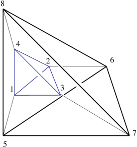
Figure 9: The Schlegel diagram of the tetrahedral prism $\Delta$. This picture can be obtained by realizing that the eight vectors $v_{i}$ describe two tetrahedrons which are separated in an extra direction. The projection used here identifies this extra direction with the radial direction in $\mathbb{R}^{3}$, i.e. we find a tetrahedron sitting inside a tetrahedron. We have labelled the vertices by their relation to the toric divisors.

Crepant resolutions of the toric fivefold (64) can be found by triangulating $\Delta$, leaving the generators $v_{i}$ untouched. As the $v_{i}$ all lie on a four-dimensional subspace, the canonical divisor of the associated toric variety is trivial both before and after the resolution. Because $u_{1}+u_{2}+u_{3}+u_{4}$ is a section of a trivial line bundle, the crepant resolutions of the ambient fivefold also induce crepant resolutions of the linear hyperplane equation given by (66). Triangulations of $\Delta$ can be found by hand or by resorting to computer algebra, such as the package TOPCOM [39]. One finds that $\Delta$ admits 24 triangulations, which we have listed in appendix A.

The corresponding 24 resolutions can also be found using algebraic equations. We introduce three $\mathbb{P}^{1}$s with homogeneous coordinates $[\xi_{1}:\xi_{2}]$, $[\zeta_{1}:\zeta_{2}]$, $[\phi_{1}:\phi_{2}]$ and replace (64) by the smooth fourfold $(\tilde{X}_{4})_{p}$:

$$y_{+}\xi_{1} =u_{p(1)}\xi_{2}$$

$$y_{-}\zeta_{1} =u_{p(2)}\zeta_{2}$$

$$\phi_{1}\xi_{2} =\phi_{2}\xi_{1}u_{p(3)}$$

$$\phi_{2}\zeta_{2} =\phi_{1}\zeta_{1}u_{p(4)}\,.$$ (70)

Here $p(k)$ denotes the $k$-th element of a permutation of the numbers $1,2,3,4$ ($p\in\mathfrak{S}_{4}$). Hence we recover the fact that we can do $4!=24$ different resolutions.

The exceptional set of the these resolutions $\rho^{\prime\prime}:(\tilde{X}_{4})_{p}\rightarrow X^{\prime}_{4}$ described above at most has a curve in $\mathbb{P}^{1}\times\mathbb{P}^{1}\times\mathbb{P}^{1}$ as the fibre over any point in the centre of the blowup, (52-57). Thus, $\rho^{\prime\prime}:(\tilde{X}_{4})_{p}\rightarrow X_{4}^{\prime}$ is a small resolution. Over all points of the base $B_{3}$, the elliptic fibre gains at most (reducible) curves, so that the fibration $\pi_{X}:(\tilde{X}_{4})_{p}\rightarrow B_{3}$ remains flat.

3.2.2 Fibre structure

Family of singular fibres over $S_{\rm GUT}$

The exceptional divisors of the blow-up of the $A_{4}$ singularity (which are divisors in $X^{\prime}_{4}$ (51) and are in the fibre of $S_{\rm GUT}$) can be expressed as the following intersections in the ambient space $\mathbb{C}^{5}$:

$$D_{1+}: \quad{\rm div}(y)\cdot{\rm div}(z)$$

$$D_{1-}: \quad{\rm div}(y+ab)\cdot{\rm div}(z)$$

$$D_{2+}: \quad{\rm div}(y)\cdot{\rm div}(x)$$

$$D_{2-}: \quad{\rm div}(y+ab+z)\cdot{\rm div}(x)\,.$$ (71)

To discuss the fibre structure, let us start by examining a particular small resolution given by the permutation $p(1,2,3,4)=(4,3,1,2)$:

$$\left(y+ab-(x+a)(x+b)\right)\xi_{1} =-x\xi_{2}$$

$$\left(y+z+(x+a)(x+b)\right)\zeta_{1} =(x+a+b)\zeta_{2}$$

$$\phi_{1}\xi_{2} =\phi_{2}\xi_{1}(x+a)$$

$$\phi_{2}\zeta_{2} =\phi_{1}\zeta_{1}(x+b)\,.$$ (72)

We will come back to discuss the geometry of singular fibres in $(\tilde{X}_{4})_{p}$ for other $p\in\mathfrak{S}_{4}$ at the end of this section 3.2.2.

For the resolution $(\tilde{X}_{4})_{p}$ with the permutation $p$ specified above, the algebraic two-parameter family of irreducible components of the singular fibre (over $S_{\rm GUT}\subset B_{3}$) become

$$D_{1+}:\hskip 56.9055pt D_{1-}:$$

$$y=z=0\hskip 56.9055pt y+ab=z=0$$

$$(x+a+b)\xi_{1}=\xi_{2}\hskip 56.9055pt x\zeta_{1}=\zeta_{2}$$

$$(x+a+b)\zeta_{2}=(x+a)(x+b)\zeta_{1}\hskip 56.9055pt (x+a)(x+b)\xi_{1}=x\xi_{2}$$

$$\phi_{1}(x+a+b)=\phi_{2}(x+a)\hskip 56.9055pt \phi_{1}\xi_{2}=\xi_{1}\phi_{2}(x+a)$$

$$\phi_{2}\zeta_{2}=\phi_{1}\zeta_{1}(x+b)\hskip 56.9055pt \phi_{2}x=\phi_{1}(x+b)$$

$$D_{2+}:\hskip 56.9055pt D_{2-}:$$

$$y=x=0\hskip 56.9055pt y+ab+z=x=0$$

$$(z+ab)\zeta_{1}=(a+b)\zeta_{2}\hskip 56.9055pt \zeta_{2}=0$$

$$\phi_{1}\xi_{2}=\xi_{1}\phi_{2}a\hskip 56.9055pt \xi_{1}=0$$

$$\phi_{2}\zeta_{2}=\phi_{1}\zeta_{1}b\hskip 56.9055pt \phi_{1}=0\,.$$ (73)

Those families are defined as subvarieties in the ambient space $\mathbb{C}^{5}\times\mathbb{P}^{1}\times\mathbb{P}^{1}\times\mathbb{P}^{1}$; five independent equations for $D_{2\pm}$ leave dimension-three subvarieties of $\tilde{X}_{4}$; the six equations for $D_{1\pm}$ are not independent, and they are still of dimension-three.

We now turn to the study of the elliptic fibre over the codimension-two loci ($\approx$ matter curves) and the codimension-three point of $E_{6}$ type. We have relegated some of the details to appendix B.

Families of singular fibres over matter curves

Let us first investigate the fibre structure over the matter curve $\Sigma_{10}:\beta_{5}|_{S_{\rm GUT}}=0$. As $\beta_{5}=ab$, this curve splits up into two irreducible components. If we focus on the branch $a=0$ we find that the divisor $D_{1+}$ splits into two four-cycles $S_{\alpha}$ and $S_{\beta}$, $D_{1-}$ splits into $S_{\beta}$ and $S_{\gamma}$, $D_{2+}$ splits into $S_{\gamma}$ and $S_{\epsilon}$ and $D_{2-}$ becomes $S_{\delta}$; see the appendix B for the definition of $S_{\alpha,\beta,\gamma,\delta,\epsilon}$. Together with the fibre component at infinity, the fibre components originating from these algebraic surfaces form an $I_{1}^{*}$ fibre over a generic point in the $a=0$ branch of the matter curve $\Sigma_{10}$. The curves $S_{\beta}$ and $S_{\gamma}$ appear with multiplicity two as expected. A similar result is obtained over the branch $b=0$.

We next turn to the fibre over the matter curve $\Sigma_{5}:\beta_{4}|_{S_{\rm GUT}}=0$. Here we denote the intersections of the exceptional divisors $D_{1+}$, $D_{1-}$ and $D_{2-}$ with ${\rm div}(\tilde{\pi}^{*}_{X}(\beta_{4}))$ in $(\tilde{X}_{4})_{p}$ by $S_{\eta}$, $S_{\kappa}$ and $S_{\lambda}$, respectively. The intersection of the divisor $D_{2+}$ with $\{a+b=0\}$ splits up into the two irreducible surface $S_{\iota}$ and $S_{\vartheta}$. See appendix B for the definitions. Hence each fibre component appears with multiplicity one. The fibre components make up a fibre of type $I_{6}$.

There is one more one-parameter algebraic family of fibre curves in $\tilde{X}_{4}$ associated with the singular locus $C_{{\rm bifund}.}$ of $X^{\prime}_{4}$. It is given by

$$S_{\tau}:\quad{\rm div}(x_{31}+a)\cdot{\rm div}(x_{31}+b)\cdot{\rm div}(y_{31}+ab)\cdot{\rm div}(y_{31}+z_{31})\cdot{\rm div}(\xi_{2})\cdot{\rm div}(\zeta_{2})$$ (74)

in the ambient space $\mathbb{C}^{5}\times\mathbb{P}^{1}\times\mathbb{P}^{1}\times\mathbb{P}^{1}$ that covers the ${\cal U}_{31}$ patch. It is a surface and is regarded as a $\mathbb{P}^{1}=\left\{[\phi_{1}:\phi_{2}]\right\}$-fibration over a curve parametrized by $a=b$. Obviously it is projected down to the curve $C_{{\rm bifund}.}$ in $X^{\prime}_{4}$, and is further mapped to a curve $(z,a,b)=(z_{31}x_{31},a,b)=(-a^{3},a,a)\subset B_{3}$.

The 1-parameter family of curves $S_{\tau}$ in $(\tilde{X}_{4})_{p}$ is associated with a transverse intersection of a pair of 7-branes (discriminant locus $\{\Delta=0\}$) in $B_{3}$ in the Weierstrass model $X_{4}^{\rm Weierstrass}$. The $I_{1}$ type fibre over such single D7-branes has nothing to do with codimension-two singularity (or with non-Abelian gauge group with 16 supercharges) and no exceptional divisor is introduced in the crepant resolution $X^{\prime}_{4}$ after the codimension-two $A_{4}$ singularity in $X_{4}^{\rm Weierstrass}$ is resolved. Over the D7-D7 transverse intersection in $B_{3}$, however, two $I_{1}$-type fibres collide, and a conifold singularity is formed. After this singularity in resolved, an algebraic surface appears in $\tilde{X}_{4}$ [40]. Since this D7-D7 intersection is away from the non-Abelian 7-branes at $z=0$ in $B_{3}$ for generic $(a,b)$, the one-parameter family $S_{\tau}$ of the singular fibre curve component stands alone, and it is not obtained as a limit of the two parameter families $D_{1\pm}$ and $D_{2\pm}$.

The singular fibre over the codimension-three locus of $E_{6}$ type

Finally, let us study the singular fibre geometry over the codimension-three point of $E_{6}$ type, characterized by $(z,a,b)=(0,0,0)\in B_{3}$. The fibre geometry at this point can be studied by taking a limit from any one of the matter curves approaching this point, but also from a generic point on $S_{\rm GUT}$. Given the discussion in section 2.2, the equivalence between these approaches is ensured by the commutativity of the Chow ring. The most convenient approach is given by starting again from the singular fibre over $S_{\rm GUT}$ (3.2.2) and intersecting them with the divisors $\{a=0\}$ and $\{b=0\}$ yielding

$$D_{1+}\, \cdot{\rm div}(\tilde{\pi}_{X}^{*}(a))\cdot{\rm div}(\tilde{\pi}_{X}^{*}(b))=\,C_{3}+C_{4}+C_{6}$$

$$D_{1-}\, \cdot{\rm div}(\tilde{\pi}_{X}^{*}(a))\cdot{\rm div}(\tilde{\pi}_{X}^{*}(b))=\,C_{2}+C_{3}+C_{6}$$

$$D_{2+}\, \cdot{\rm div}(\tilde{\pi}_{X}^{*}(a))\cdot{\rm div}(\tilde{\pi}_{X}^{*}(b))=\,C_{2}+C_{3}+C_{4}+C_{5}$$

$$D_{2-}\, \cdot{\rm div}(\tilde{\pi}_{X}^{*}(a))\cdot{\rm div}(\tilde{\pi}_{X}^{*}(b))=\,C_{1}$$ (75)

in terms of the irreducible curves

$$C_{1}:\quad {\rm div}(y+z)\cdot{\rm div}(x)\cdot{\rm div}(\zeta_{2})\cdot{\rm div}(\xi_{1})\cdot{\rm div}(\phi_{1})$$

$$C_{2}:\quad {\rm div}(y)\cdot{\rm div}(x)\cdot{\rm div}(z)\cdot{\rm div}(\phi_{1})\cdot{\rm div}(\zeta_{2})$$

$$C_{3}:\quad {\rm div}(y)\cdot{\rm div}(x)\cdot{\rm div}(z)\cdot{\rm div}(\xi_{2})\cdot{\rm div}(\zeta_{2})$$

$$C_{4}:\quad {\rm div}(y)\cdot{\rm div}(x)\cdot{\rm div}(z)\cdot{\rm div}(\xi_{2})\cdot{\rm div}(\phi_{2})$$

$$C_{5}:\quad {\rm div}(y)\cdot{\rm div}(x)\cdot{\rm div}(\zeta_{1})\cdot{\rm div}(\phi_{2})\cdot{\rm div}(\xi_{2})$$

$$C_{6}:\quad {\rm div}(z)\cdot{\rm div}(y)\cdot{\rm div}(x\xi_{1}-\xi_{2})\cdot{\rm div}(\phi_{1}-\phi_{2})\cdot{\rm div}(x\zeta_{1}-\zeta_{2})$$ (76)

in $\mathbb{C}^{5}|_{(a,b)=(0,0)}\times\mathbb{P}^{1}\times\mathbb{P}^{1}\times\mathbb{P}^{1}$. We have dropped the factors ${\rm div}(\tilde{\pi}_{X}^{*}(a))\cdot{\rm div}(\tilde{\pi}_{X}^{*}(b))$ which are common to all of the above. The curves $C_{1,\cdots,6}$ appear with the multiplicity assigned for the roots of $E_{6}$, and share points with one another in the way shown in fig. 10, which looks the same as the IV^∗ type fibre in Kodaira’s classification.

Figure 10: The geometry of irreducible components in the singular fibre over the codimension-three point of $E_{6}$ type.

Twenty-three resolutions more

Before concluding this section, we would like to comment on the dependence of our findings on which permutation $p(k)$ is used. One of the results of [1] was that the form of the fibre over the $E_{6}$ Yukawa point is not the same for all the different small resolutions. It is known that any small resolutions of a given singularity have the same Hodge numbers [20]. This is not enough, however, to ensure that the fibre geometry are the same for all the small resolutions; the study of [1] shows clearly that such a phenomenon indeed happens for $SU(5)$ models with generic complex structure. In the case of linear Higgs vev, we have so far studied the singular fibre geometry only for one of the twenty-four small resolutions. Thus, we have to work on twenty-three other resolutions separately.

It is not difficult to see, however, that the singular fibre geometry over the $E_{6}$-type point remains the same for all twenty-four small resolutions. An important point is that we can specialize the problem in the $a=b=0$ locus first; setting $a=b=0$, $u_{1,2}=x$ and $u_{3,4}=-x$, which greatly simplifies the problem. The fibre geometry for the resolution with $p(1,2,3,4)=(4,3,1,2)$ becomes (3.2.1) becomes

$$y_{+}\xi_{1} =-x\xi_{2}$$

$$y_{-}\zeta_{1} =-x\zeta_{2}$$

$$\phi_{1}\xi_{2} =\phi_{2}\xi_{1}x$$

$$\phi_{2}\zeta_{2} =\phi_{1}\zeta_{1}x\,.$$ (77)

For other $p\in\mathfrak{S}_{4}$, the minus signs on the right hand side appear in other places. One can construct isomorphisms among these fibre geometries for different $p\in\mathfrak{S}_{4}$’s, by choosing one of the eight options:

$$([\xi_{1}:\xi_{2}],[\zeta_{1}:\zeta_{2}],[\phi_{1}:\phi_{2}])\mapsto([\pm\xi_{1}:\xi_{2}],[\pm\zeta_{1}:\zeta_{2}],[\pm\phi_{1}:\phi_{2}]).$$ (78)

Therefore, in the case of linear Higgs vev, the singular fibre geometry over the $E_{6}$ type point remains the same for all the twenty-four different resolutions $\tilde{X}_{4}$ satisfying condition (e).

3.3 The codimension-three locus of $E_{7}$-type for $SO(10)$ models

We have already seen that the singular fibre in the resolved geometry $\tilde{X}_{4}$ under the condition (e) follow the empirical rule we proposed in section 2.3, when the complex structure of $X_{4}^{\rm Weierstrass}$ is chosen so that the Higgs vev is linear in the local coordinates around codimension-three points of $A_{4}$ type and $E_{6}$-type in $SU(5)$ models. At the end of this article, we briefly mention how to carry out similar experiment for the codimension-three points of $E_{7}$ type in $SO(10)$ models. This does not involve extra complications, but we will leave the explicit analysis as an open problem.

As a local geometry of $X_{4}^{\rm Weierstrass}$ of $SO(10)$ models, we can think of $X_{4}^{({\rm Weierstrass})}$ given by (3) with

$$\beta_{3}=a+b\,,\quad\beta_{4}=ab\,,\quad\beta_{0}=\beta^{\prime}_{5}=0\,,\quad\beta_{2}=1$$ (79)

in order to realize a linear Higgs vev in the vicinity of an $E_{7}$-type point. This special choice of complex structure worsens the singularity of $X^{\prime}_{4}$ for $SO(10)$ models in patch ${\cal U}_{313}$, (13), which for a linear Higgs vev reads

$$y_{313}(y_{313}+a+b)=x_{313}(x_{313}z_{313}+ab+z_{313})\,.$$ (80)

Besides the obvious conifold singularity, which we have already encountered in section 2.1, there is now also a singularity along

$$a=b=-y_{313}\,,\quad x_{313}=-1\,,\quad z_{313}=b^{2}\,,$$ (83)

which is in the fibre of $\left\{(z,a,b)=(z_{313}^{2}x_{313},a,b)=(-b^{4},b,b)|{}^{\forall}b\right\}\subset B_{3}$, precisely at the place we expect from the locus of intersection of factorized spectral surface $(\xi-a)(\xi-b)=0$.

The conifold singularity over the $SO(10)$-${\bf 10}$-representation matter curve and this new singular locus of $X^{\prime}_{4}$ can be treated in a symmetric way, once we rewrite the equation (80) as

$$\left(y_{313}+a+b(x_{313}+1)\right)\left(y_{313}-x_{313}b\right)=x_{313}(x_{313}+1)(z_{313}-b^{2})\,$$ (84)

or

$$\left(y_{313}+b+a(x_{313}+1)\right)\left(y_{313}-x_{313}a\right)=x_{313}(x_{313}+1)(z_{313}-a^{2})\,.$$ (85)

If we are to denote the two factors in the left-hand sides as $y_{\pm}$, then the two curves of conifold singularity correspond to $y_{+}=y_{-}=x_{313}=(z_{313}-b^{2})=0$ and $y_{+}=y_{-}=(x_{313}+1)=(z_{313}-b^{2})=0$, respectively.

As we have not worked out possible resolutions under the condition (e) for this geometry, we are not in a position to conclude that the empirical rule in section 2.3 holds true for the case of $E_{7}$-type points in $SO(10)$ models with linear Higgs background. A similar analysis can be carried out for the $D_{7}$ type points of $SO(10)$ models or $E_{8}$-type points of $E_{6}$ models with linear Higgs background as well (see [14, 15] for the necessary information).

In between the linear Higgs background (trivial 7-brane monodromy) and the full $\mathfrak{S}_{r}$ monodromy of an $r$-fold spectral cover, one can think of many different choices of monodromy groups [33, 41, 42, 43, 31]. It will be interesting to carry out the resolution under the condition (e) and study the singular fibres for such geometries. The results can be used as experimental data for testing the empirical rule in section 2.3, and to think more about the possibility hinted at the end of section 2.3. With such an experimental approach, the empirical rule may be promoted to a dictionary between the singular fibres of $X_{n}$ under the condition (e) and symmetries unbroken at the corresponding points in the base (or some other physics concepts); it will even be possible to refine the dictionary, based on more data. All these things, however, are beyond the scope of this article.

Acknowledgements

We have benefited from discussions with Radu Tatar and William Walters, with whom we worked together at the earlier stage of this project. TW thanks the organizers of CERN theory institute in 2012 summer for providing such an opportunity. We thank Alexey Bondal and Satoshi Kondo for useful comments. A. P. B. likes to thank the IPMU Tokyo for kind hospitality during his visit. The work of A. P. B. was supported by a JSPS postdoctoral fellowship under grant PE 12530 and by the STFC under grant ST/J002798/1. The work of T. W. was supported by WPI Initiative, MEXT, Japan and a Grant-in-Aid for Scientific Research on Innovative Areas 2303.

Appendix A Triangulations and resolutions of the toric fivefold

In this appendix, we record some technical details regarding the possible small resolutions of the fourfold (51). As discussed in section 3.2.1, this space is realized as the hypersurface $u_{1}+u_{2}+u_{3}+u_{4}=0$ in the toric fivefold

$$y_{+}y_{-}=u_{1}u_{2}u_{3}u_{4}\,.$$ (86)

The toric variety corresponding to this algebraic equation has a fan which just contains a single five-dimensional non-simplicial cone $\Sigma$ over a polytope $\Delta$, see also fig. 9. This cone is generated by the vectors $v_{1,2,\cdots,8}$ in (67).

$\#$	$\Sigma_{i}$ are generated by	refinement of
$1$	$\{1,2,3,4,5\},\{2,3,4,5,6\},\{3,4,5,6,7\},\{4,5,6,7,8\}$	${\cal E}_{xw}$
$2$	$\{1,2,3,4,5\},\{2,3,4,5,6\},\{3,4,5,6,8\},\{3,5,6,7,8\}$	${\cal E}_{tw}$
$3$	$\{1,2,3,4,5\},\{2,3,4,5,7\},\{2,4,5,6,7\},\{4,5,6,7,8\}$
$4$	$\{1,2,3,4,5\},\{2,3,4,5,7\},\{2,4,5,7,8\},\{2,5,6,7,8\}$
$5$	$\{1,2,3,4,5\},\{2,3,4,5,8\},\{2,3,5,6,8\},\{3,5,6,7,8\}$
$6$	$\{1,2,3,4,5\},\{2,3,4,5,8\},\{2,3,5,7,8\},\{2,5,6,7,8\}$
$7$	$\{1,2,3,4,6\},\{1,3,4,5,6\},\{3,4,5,6,7\},\{4,5,6,7,8\}$	${\cal E}_{xw}$
$8$	$\{1,2,3,4,6\},\{1,3,4,5,6\},\{3,4,5,6,8\},\{3,5,6,7,8\}$	${\cal E}_{tw}$
$9$	$\{1,2,3,4,6\},\{1,3,4,6,7\},\{1,4,5,6,7\},\{4,5,6,7,8\}$
$10$	$\{1,2,3,4,6\},\{1,3,4,6,7\},\{1,4,6,7,8\},\{1,5,6,7,8\}$
$11$	$\{1,2,3,4,6\},\{1,3,4,6,8\},\{1,3,5,6,8\},\{3,5,6,7,8\}$
$12$	$\{1,2,3,4,6\},\{1,3,4,6,8\},\{1,3,6,7,8\},\{1,5,6,7,8\}$
$13$	$\{1,2,3,4,7\},\{1,2,4,5,7\},\{2,4,5,6,7\},\{4,5,6,7,8\}$	${\cal E}_{xt}$
$14$	$\{1,2,3,4,7\},\{1,2,4,5,7\},\{2,4,5,7,8\},\{2,5,6,7,8\}$
$15$	$\{1,2,3,4,7\},\{1,2,4,6,7\},\{1,4,5,6,7\},\{4,5,6,7,8\}$	${\cal E}_{xt}$
$16$	$\{1,2,3,4,7\},\{1,2,4,6,7\},\{1,4,6,7,8\},\{1,5,6,7,8\}$
$17$	$\{1,2,3,4,7\},\{1,2,4,7,8\},\{1,2,5,7,8\},\{2,5,6,7,8\}$	${\cal E}_{wt}$
$18$	$\{1,2,3,4,7\},\{1,2,4,7,8\},\{1,2,6,7,8\},\{1,5,6,7,8\}$	${\cal E}_{wt}$
$19$	$\{1,2,3,4,8\},\{1,2,3,5,8\},\{2,3,5,6,8\},\{3,5,6,7,8\}$	${\cal E}_{tx}$
$20$	$\{1,2,3,4,8\},\{1,2,3,5,8\},\{2,3,5,7,8\},\{2,5,6,7,8\}$
$21$	$\{1,2,3,4,8\},\{1,2,3,6,8\},\{1,3,5,6,8\},\{3,5,6,7,8\}$	${\cal E}_{tx}$
$22$	$\{1,2,3,4,8\},\{1,2,3,6,8\},\{1,3,6,7,8\},\{1,5,6,7,8\}$
$23$	$\{1,2,3,4,8\},\{1,2,3,7,8\},\{1,2,5,7,8\},\{2,5,6,7,8\}$	${\cal E}_{wx}$
$24$	$\{1,2,3,4,8\},\{1,2,3,7,8\},\{1,2,6,7,8\},\{1,5,6,7,8\}$	${\cal E}_{wx}$

Table 5: The 24 triangulations of $\Delta$. Each triangulation subdivides the cone over $\Delta$ into four simplicial cones, each of which is spanned by five vectors $v_{i}$. Each row in the table above describes a single triangulation. For each triangulation, we have collected the generators $v_{i}$ spanning each four five-dimensional cone in curly brackets $\{\cdots\}$. For the sake of brevity, we merely write $i$ instead of $v_{i}$. E.g. for the first triangulation, the four different five-dimensional cones are generated by $\Sigma_{1}=\langle v_{1},v_{2},v_{3},v_{4},v_{5}\rangle$, $\Sigma_{2}=\langle v_{2},v_{3},v_{4},v_{5},v_{6}\rangle$, $\Sigma_{3}=\langle v_{3},v_{4},v_{5},v_{6},v_{7}\rangle$ and $\Sigma_{4}=\langle v_{4},v_{5},v_{6},v_{7},v_{8}\rangle$. The lower dimensional cones in each triangulation are faces of the $\Sigma_{i}$. Each of these triangulations corresponds to a small morphism. In the right column, we have indicated which of these morphisms can be obtained by first applying one of the $6$ small morphisms of [1], followed by a small resolution of the remaining singularity.

In order to turn this into a smooth toric variety, we must completely triangulate $\Delta$. Any such triangulation turns $\Delta$ into four four-dimensional cells $\hat{\Delta}_{i}$ and subdivides $\Sigma$ into the four simplicial cones $\Sigma_{i}$. In table 5, we have listed the $24$ triangulations of $\Delta$ by giving the vectors $v_{i}$ spanning the simplicial cones $\Sigma_{i}$ over the $\hat{\Delta}_{i}$ resulting from the triangulation.

Using the following identification of coordinates:

$$y_{+} =y+ab-(x+a)(x+b)=z_{1}z_{2}z_{3}z_{4}$$

$$y_{-} =-\left(y+z+(x+a)(x+b)\right)=z_{5}z_{6}z_{7}z_{8}$$

$$u_{1} =x+a=z_{1}z_{5}$$

$$u_{2} =x+b=z_{2}z_{6}$$

$$u_{3} =-\left(x+a+b\right)=z_{3}z_{7}$$

$$u_{4} =-x=z_{4}z_{8}\,,$$ (87)

and examining the intersection ring, we can map the $24$ triangulations to the $24$ resolutions that were obtained using algebraic equations. Given (3.2.1) with $p\in\mathfrak{S}_{4}$, this corresponds to the triangulation $\Sigma_{1}=\left\langle{v_{1,2,3,4},v_{p(2)}}\right\rangle$, $\Sigma_{2}=\left\langle{v_{p(1,3,4)},v_{4+p(2,4)}}\right\rangle$, $\Sigma_{3}=\left\langle{v_{p(1,3)},v_{4+p(2,3,4)}}\right\rangle$, $\Sigma_{4}=\left\langle{v_{p(1)},v_{5,6,7,8}}\right\rangle$ in table 5.

We can arrive at $12$ of these by starting from (51) and applying one of the six small morphisms ${\cal E}_{ij}$ used in [1]. These morphisms correspond to a partial triangulation of $\Delta$, so that they do not completely resolve the singularities of (51). It turns out that they leave a curve of conifold singularities, which can be resolved by a further small resolution (for which there are the usual two choices). After performing one of the two small resolutions we obtain a smooth fourfold corresponding to one of the $24$ triangulations in table 5. The triangulations which can be obtained this way are listed in the right column.

Appendix B One-parameter families of fibre components for a $SU(5)$ GUT model with linear higgs field

In this appendix, we list expressions for the various algebraic submanifolds appearing in section 3.2.2.

The matter curve of $SU(5)$-${\bf 10}+\overline{\bf 10}$ representation splits into two components, $a=0$ and $b=0$ in the case of linear Higgs background (48). In the fibre of the $a=0$ curve in $S_{\rm GUT}$, we can construct multiple families of fibre components parametrized by the local coordinate $b$ of the curve. They are given by

$$S_{\alpha}:\quad {\rm div}(z)\cdot{\rm div}(y)\cdot{\rm div}(\phi_{2})\cdot{\rm div}(x+b)\cdot{\rm div}(\xi_{2})$$

$$S_{\beta}:\quad {\rm div}(z)\cdot{\rm div}(y)\cdot{\rm div}(\xi_{2}-\xi_{1}(x+b))\cdot{\rm div}(x\zeta_{1}-\zeta_{2})\cdot{\rm div}(\phi_{2}x-\phi_{1}(x+b))$$

$$S_{\gamma}:\quad {\rm div}(z)\cdot{\rm div}(y)\cdot{\rm div}(\phi_{1})\cdot{\rm div}(x)\cdot{\rm div}(\zeta_{2})$$

$$S_{\delta}:\quad {\rm div}(y+z)\cdot{\rm div}(x)\cdot{\rm div}(\xi_{1})\cdot{\rm div}(\zeta_{2})\cdot{\rm div}(\phi_{1})$$

$$S_{\epsilon}:\quad {\rm div}(y)\cdot{\rm div}(x)\cdot{\rm div}(z\zeta_{1}-b\zeta_{2})\cdot{\rm div}(\xi_{2})\cdot{\rm div}(\phi_{2}\zeta_{2}-\phi_{1}\zeta_{1}b)$$ (88)

in the ambient space $\mathbb{C}^{5}\times\mathbb{P}^{1}\times\mathbb{P}^{1}\times\mathbb{P}^{1}$, where ${\rm div}(a)$, common to all above, has been omitted. Six equations in the eight-dimensional ambient space leave a complex two-dimensional variety, which sits within $(\tilde{X}_{4})_{p}$ given by (3.2.2).

Similarly, two-dimensional subvarieties of $(\tilde{X}_{4})_{p}$ exist in the fibre of the other branch of the matter curve, $b=0$.

$$S_{\alpha}^{\prime}:\quad {\rm div}(z)\cdot{\rm div}(y)\cdot{\rm div}(\xi_{2})\cdot{\rm div}(x+a)\cdot{\rm div}(\phi_{2}\zeta_{2}-\phi_{1}\zeta_{1}x)$$

$$S_{\beta}^{\prime}:\quad {\rm div}(z)\cdot{\rm div}(y)\cdot{\rm div}(\xi_{2}-\xi_{1}(x+a))\cdot{\rm div}(x\zeta_{1}-\zeta_{2})\cdot{\rm div}(\phi_{2}-\phi_{1})$$

$$S_{\gamma}^{\prime}:\quad {\rm div}(z)\cdot{\rm div}(y)\cdot{\rm div}(\zeta_{2})\cdot{\rm div}(x)\cdot{\rm div}(\phi_{1}\xi_{2}-\xi_{1}\phi_{2}a)$$

$$S_{\delta}^{\prime}:\quad {\rm div}(y+z)\cdot{\rm div}(x)\cdot{\rm div}(\xi_{1})\cdot{\rm div}(\zeta_{2})\cdot{\rm div}(\phi_{1})$$

$$S_{\epsilon}^{\prime}:\quad {\rm div}(y)\cdot{\rm div}(x)\cdot{\rm div}(z\zeta_{1}-a\zeta_{2})\cdot{\rm div}(\xi_{2})\cdot{\rm div}(\phi_{2}),$$ (89)

where we have omitted ${\rm div}(b)$ which is common to all above.

The surfaces over the ${\bf 5}$ matter curve $a+b=0$ are given by

$$S_{\eta}:\quad {\rm div}(z)\cdot{\rm div}(y)\cdot{\rm div}(x\xi_{1}-\xi_{2})\cdot{\rm div}\left(x\zeta_{2}-(x+a)(x+b)\zeta_{1}\right)\cdot{\rm div}\left(x\phi_{1}-\phi_{2}(x+a)\right)$$

$$S_{\kappa}:\quad {\rm div}(z)\cdot{\rm div}(y+ab)\cdot{\rm div}\left(\zeta_{2}-\zeta_{1}x\right)\cdot{\rm div}\left(x\xi_{2}-(x+a)(x+b)\xi_{1}\right)\cdot{\rm div}\left(\phi_{2}x-\phi_{1}(x+b)\right)$$

$$S_{\iota}:\quad {\rm div}(y)\cdot{\rm div}(x)\cdot{\rm div}(z+ab)\cdot{\rm div}(\phi_{1}\xi_{2}-\xi_{1}\phi_{2}a)\cdot{\rm div}(\phi_{2}\zeta_{2}-\phi_{1}\zeta_{1}b)$$

$$S_{\vartheta}:\quad {\rm div}(y)\cdot{\rm div}(x)\cdot{\rm div}(\xi_{2})\cdot{\rm div}(\zeta_{1})\cdot{\rm div}(\phi_{2})$$

$$S_{\lambda}:\quad {\rm div}(y+ab+z)\cdot{\rm div}(x)\cdot{\rm div}(\zeta_{2})\cdot{\rm div}(\xi_{1})\cdot{\rm div}(\phi_{1})\,.$$ (90)

We have omitted the factor ${\rm div}(a+b)$, which is common to all above.

The Yukawa coupling analysis of [5] in our language corresponds to proving that

$$\left[S_{\alpha}\right]\cdot{\rm div}(\tilde{\pi}_{X}^{*}(b))+\left[S_{\vartheta}\right]\cdot{\rm div}(\tilde{\pi}_{X}^{*}(a))-\left[S^{\prime}_{\epsilon}\right]\cdot{\rm div}(\tilde{\pi}_{X}^{*}(a)) \equiv 0\,,$$ (91)

$$\left[S_{\alpha}\right]\cdot{\rm div}(\tilde{\pi}_{X}^{*}(b))-\left[S^{\prime}_{\alpha}\right]\cdot{\rm div}(\tilde{\pi}_{X}^{*}(a))+S_{\tau}\cdot{\rm div}(\tilde{\pi}_{X}^{*}(a)) \equiv 0\,,$$ (92)

modulo $D_{1\pm,2\pm}\cdot{\rm div}\left(\tilde{\pi}_{X}^{*}(a)\right)\cdot{\rm div}\left(\tilde{\pi}_{X}^{*}(b)\right)$. Here, $[S_{\alpha}]$ is the equivalence class of $S_{\alpha}$ in the quotient space

$${\rm Span}_{\mathbb{Z}}\left\{S_{\alpha,\beta,\gamma,\delta,\epsilon}\right\}/{\rm Span}_{\mathbb{Z}}\left\{D_{1\pm,2\pm}\cdot{\rm div}(\tilde{\pi}_{X}^{*}(a))\right\},$$ (93)

and $[S^{\prime}_{\alpha}]=-[S^{\prime}_{\epsilon}]$ and $[S_{\vartheta}]$ are the equivalence classes for the corresponding matter curves. The class $S_{\tau}$ is given in (74). The relations above hold because

$$S_{\alpha}\cdot{\rm div}(\tilde{\pi}_{X}^{*}(b))=C_{4},\quad S^{\prime}_{\alpha}\cdot{\rm div}(\tilde{\pi}_{X}^{*}(a))=C_{3}+C_{4},\quad S^{\prime}_{\epsilon}\cdot{\rm div}(\tilde{\pi}_{X}^{*}(a))=C_{4}+C_{5},$$

$$S_{\vartheta}\cdot{\rm div}(\tilde{\pi}_{X}^{*}(a))=C_{5},\quad S_{\tau}\cdot{\rm div}(\tilde{\pi}_{X}^{*}(a))=C_{3}.$$ (94)

The generation of Yukawa couplings around codimension-three singularities can be understood at the intuitive level in the language of M2-branes wrapped on 2-cycles in the ALE-fibre of A-D-E type [33, 14], and the field theory local models provide a formulation of quantitative calculation of F-term Yukawa couplings [11, 12, 13, 15, 16]. Therefore, the confirmation of the topological relations among 2-cycles (91, 92) does not introduce new ingredients to the calculation of Yukawa couplings. Because of localization of F-term Yukawa couplings in supersymmetric compactifications [44] (see also [45]), however, we feel comfortable to repeat, in the language of algebraic geometry, the confirmation of the topological relations in the deformed A-D-E fibration [33]. This comfortable confirmation can be regarded as a non-negative evidnece for the choice of the condition (e) [5].

References

- [1] M. Esole and S.-T. Yau, “Small resolutions of SU(5)-models in F-theory,” arXiv:1107.0733 [hep-th].
- [2] T. Hübsch, Calabi-Yau manifolds. A bestiary for physicists. World Scientific, Singapore, 1991.
- [3] D. R. Morrison and C. Vafa, “Compactifications of F theory on Calabi-Yau threefolds. 2.,” Nucl.Phys. B476 (1996) 437–469, arXiv:hep-th/9603161 [hep-th].
- [4] M. Bershadsky, K. A. Intriligator, S. Kachru, D. R. Morrison, V. Sadov, et al., “Geometric singularities and enhanced gauge symmetries,” Nucl.Phys. B481 (1996) 215–252, arXiv:hep-th/9605200 [hep-th].
- [5] J. Marsano and S. Schafer-Nameki, “Yukawas, G-flux, and Spectral Covers from Resolved Calabi-Yau’s,” JHEP 1111 (2011) 098, arXiv:1108.1794 [hep-th].
- [6] K. Kodaira, “On compact analytic surfaces: ii,” Annals of Mathematics 77 no. 3, (1963) pp. 563–626.
- [7] K. Kodaira, “On compact analytic surfaces, iii,” Annals of Mathematics 78 no. 1, (1963) pp. 1–40.
- [8] W. Barth, C. Peters, and A. van de Ven, Compact complex surfaces. Springer-Verlag, 1984.
- [9] J. Tate, “Algorithm for determining the type of a singular fiber in an elliptic pencil,” in Modular Functions of One Variable IV, B. Birch and W. Kuyk, eds., vol. 476 of Lecture Notes in Mathematics, pp. 33–52. Springer Berlin / Heidelberg, 1975. http://dx.doi.org/10.1007/BFb0097582. 10.1007/BFb0097582.
- [10] S. Katz, D. R. Morrison, S. Schafer-Nameki, and J. Sully, “Tate’s algorithm and F-theory,” JHEP 1108 (2011) 094, arXiv:1106.3854 [hep-th].
- [11] S. H. Katz and C. Vafa, “Matter from geometry,” Nucl. Phys. B497 (1997) 146–154, arXiv:hep-th/9606086.
- [12] R. Donagi and M. Wijnholt, “Model Building with F-Theory,” arXiv:0802.2969 [hep-th].
- [13] C. Beasley, J. J. Heckman, and C. Vafa, “GUTs and Exceptional Branes in F-theory - I,” JHEP 01 (2009) 058, arXiv:0802.3391 [hep-th].
- [14] H. Hayashi, R. Tatar, Y. Toda, T. Watari, and M. Yamazaki, “New Aspects of Heterotic–F Theory Duality,” Nucl. Phys. B806 (2009) 224–299, arXiv:0805.1057 [hep-th].
- [15] H. Hayashi, T. Kawano, R. Tatar, and T. Watari, “Codimension-3 Singularities and Yukawa Couplings in F- theory,” Nucl. Phys. B823 (2009) 47–115, arXiv:0901.4941 [hep-th].
- [16] H. Hayashi, T. Kawano, Y. Tsuchiya, and T. Watari, “Flavor Structure in F-theory Compactifications,” JHEP 08 (2010) 036, arXiv:0910.2762 [hep-th].
- [17] S. Cecotti, C. Cordova, J. J. Heckman, and C. Vafa, “T-Branes and Monodromy,” JHEP 1107 (2011) 030, arXiv:1010.5780 [hep-th].
- [18] T. Kawano, Y. Tsuchiya, and T. Watari, “A Note on Kahler Potential of Charged Matter in F-theory,” Phys.Lett. B709 (2012) 254–259, arXiv:1112.2987 [hep-th].
- [19] B. Andreas and G. Curio, “On discrete twist and four flux in N=1 heterotic / F theory compactifications,” Adv.Theor.Math.Phys. 3 (1999) 1325–1413, arXiv:hep-th/9908193 [hep-th].
- [20] V. V. Batyrev, “Birational Calabi–Yau n-folds have equal Betti numbers,” in New trends in algebraic geometry (Warwick, 1996), vol. 264, pp. 1–11. Cambridge Univ. Press, Cambridge, 1999. arXiv:alg-geom/9710020.
- [21] C. Lawrie and S. Schafer-Nameki, “The Tate Form on Steroids: Resolution and Higher Codimension Fibers,” arXiv:1212.2949 [hep-th].
- [22] R. Tatar and W. Walters, “GUT theories from Calabi-Yau 4-folds with SO(10) Singularities,” arXiv:1206.5090 [hep-th].
- [23] S. Krause, C. Mayrhofer, and T. Weigand, “ flux, chiral matter and singularity resolution in F-theory compactifications,” Nucl.Phys. B858 (2012) 1–47, arXiv:1109.3454 [hep-th].
- [24] R. Blumenhagen, T. W. Grimm, B. Jurke, and T. Weigand, “Global F-theory GUTs,” Nucl.Phys. B829 (2010) 325–369, arXiv:0908.1784 [hep-th].
- [25] T. W. Grimm, S. Krause, and T. Weigand, “F-Theory GUT Vacua on Compact Calabi-Yau Fourfolds,” JHEP 1007 (2010) 037, arXiv:0912.3524 [hep-th].
- [26] A. Collinucci and R. Savelli, “On Flux Quantization in F-Theory,” JHEP 1202 (2012) 015, arXiv:1011.6388 [hep-th].
- [27] J. Knapp, M. Kreuzer, C. Mayrhofer, and N.-O. Walliser, “Toric Construction of Global F-Theory GUTs,” JHEP 1103 (2011) 138, arXiv:1101.4908 [hep-th].
- [28] A. Collinucci and R. Savelli, “On Flux Quantization in F-Theory II: Unitary and Symplectic Gauge Groups,” JHEP 1208 (2012) 094, arXiv:1203.4542 [hep-th].
- [29] J. Marsano, N. Saulina, and S. Schafer-Nameki, “F-theory Compactifications for Supersymmetric GUTs,” JHEP 0908 (2009) 030, arXiv:0904.3932 [hep-th].
- [30] P. S. Aspinwall and M. Gross, “The SO(32) heterotic string on a K3 surface,” Phys.Lett. B387 (1996) 735–742, arXiv:hep-th/9605131 [hep-th].
- [31] H. Hayashi, T. Kawano, Y. Tsuchiya, and T. Watari, “More on Dimension-4 Proton Decay Problem in F-theory – Spectral Surface, Discriminant Locus and Monodromy,” Nucl. Phys. B840 (2010) 304–348, arXiv:1004.3870 [hep-th].
- [32] R. Donagi and M. Wijnholt, “Breaking GUT Groups in F-Theory,” Adv.Theor.Math.Phys. 15 (2011) 1523–1604, arXiv:0808.2223 [hep-th].
- [33] R. Tatar and T. Watari, “Proton decay, Yukawa couplings and underlying gauge symmetry in string theory,” Nucl.Phys. B747 (2006) 212–265, arXiv:hep-th/0602238 [hep-th].
- [34] R. Donagi and D. Gaitsgory, “The Gerbe of Higgs bundles,” Transform. Groups 7 (2002) 109–153, arXiv:math/0005132 [math-ag].
- [35] R. Tatar, Y. Tsuchiya, and T. Watari, “Right-handed Neutrinos in F-theory Compactifications,” Nucl. Phys. B823 (2009) 1–46, arXiv:0905.2289 [hep-th].
- [36] T. W. Grimm and T. Weigand, “On Abelian Gauge Symmetries and Proton Decay in Global F- theory GUTs,” Phys. Rev. D82 (2010) 086009, arXiv:1006.0226 [hep-th].
- [37] K.-S. Choi and H. Hayashi, “U(n) Spectral Covers from Decomposition,” JHEP 1206 (2012) 009, arXiv:1203.3812 [hep-th].
- [38] C. Mayrhofer, E. Palti, and T. Weigand, “U(1) symmetries in F-theory GUTs with multiple sections,” arXiv:1211.6742 [hep-th].
- [39] J. Rambau, “TOPCOM: Triangulations of point configurations and oriented matroids,” in Mathematical Software—ICMS 2002, A. M. Cohen, X.-S. Gao, and N. Takayama, eds., pp. 330–340. World Scientific, 2002. http://www.zib.de/PaperWeb/abstracts/ZR-02-17.
- [40] A. P. Braun, A. Collinucci, and R. Valandro, “G-flux in F-theory and algebraic cycles,” Nucl.Phys. B856 (2012) 129–179, arXiv:1107.5337 [hep-th].
- [41] V. Bouchard, J. J. Heckman, J. Seo, and C. Vafa, “F-theory and Neutrinos: Kaluza-Klein Dilution of Flavor Hierarchy,” JHEP 1001 (2010) 061, arXiv:0904.1419 [hep-ph].
- [42] J. J. Heckman, A. Tavanfar, and C. Vafa, “The Point of E(8) in F-theory GUTs,” JHEP 1008 (2010) 040, arXiv:0906.0581 [hep-th].
- [43] J. Marsano, N. Saulina, and S. Schafer-Nameki, “Monodromies, Fluxes, and Compact Three-Generation F-theory GUTs,” JHEP 0908 (2009) 046, arXiv:0906.4672 [hep-th].
- [44] S. Cecotti, M. C. N. Cheng, J. J. Heckman, and C. Vafa, “Yukawa Couplings in F-theory and Non-Commutative Geometry,” arXiv:0910.0477 [hep-th].
- [45] J. P. Conlon and E. Palti, “Aspects of Flavour and Supersymmetry in F-theory GUTs,” JHEP 1001 (2010) 029, arXiv:0910.2413 [hep-th].