Avalanches, Breathers and Flow Reversal in a Continuous Lorenz-96 Model

Abstract

For the discrete model suggested by Lorenz in 1996 a one-dimensional long wave approximation with nonlinear excitation and diffusion is derived. The model is energy conserving but non-Hamiltonian. In a low order truncation weak external forcing of the zonal mean flow induces avalanche-like breather solutions which cause reversal of the mean flow by a wave-mean flow interaction. The mechanism is an outburst-recharge process similar to avalanches in a sand pile model.

In 1996 Lorenz suggested a nonlinear chaotic model for an unspecified observable with next and second nearest neighbor couplings on grid points along a latitude circle Lorenz (1996). Due to its scalability the model is a versatile tool in statistical mechanics Abramov and Majda (2007); Hallerberg et al. (2010); Lucarini (2012); Lucarini and Sarno (2011) and meteorology Ambadan and Tang (2009); Khare and Smith (2011); Messner and Mayr (2011). The nonlinear terms have a quadratic conservation law and satisfy Liouville’s Theorem. For strong forcing the model shows intermittency Lorenz (2006).

The Lorenz-96 equations for the variable $X_{i}$ are a surrogate for nonlinear advection in a periodic domain

$$\frac{d}{dt}X_{i}=X_{i-1}[X_{i+1}-X_{i-2}]-\gamma X_{i}+F_{i}$$ (1)

$\gamma$ characterizes linear friction ($\gamma=1$ in Lorenz (1996)) and $F$ is a forcing.

In this Letter a continuous long wave approximation of the Lorenz-96 model is derived. A surprising finding is that the nonlinear terms in the Taylor expansion are associated with generic dynamic operators. Furthermore, the dynamics in a truncated version reveals avalanches, breather-like excitations and flow reversals, which mimic various physical processes in complex systems in a simplistic way.

Lorenz Lorenz (2005) has analysed the linear stability of the mean $m$ of $X_{i}$ in (1) and found that long waves with wave numbers $k<2\pi/3$ are unstable for a positive mean $m$.

For $\gamma=F=0$ the equations (1) are conservative with the conservation law, $H_{X}=1/2\sum_{i}X_{i}^{2}$, denoted as energy in the following. The dynamics in the state space of the $X_{i}$ is non-divergent thus satisfying Liouville’s Theorem, $\sum_{i}\partial\dot{X}_{i}/\partial X_{i}=0$.

The dynamics of an observable function $Q(X)$ is given by

$$Q_{t}=\{Q,H_{X}\}$$ (2)

with an anti-symmetric bracket

$$\{A,B\}=\partial_{i}AJ_{ij}\partial_{j}B=-\{B,A\}$$ (3)

and the antisymmetric matrix

$$J_{ij}=X_{i-1}\delta_{j,i+1}-X_{j-1}\delta_{i,j+1}$$ (4)

Energy $H_{X}$ is conserved due to the anti-symmetry of the bracket.

The conservative terms of the Lorenz-96 equations (1) are obtained for $Q=X_{i}$. The equations are non-Hamiltonian Sergi and Ferrario (2001) since the Jacobi identity

$$\sum_{\ell}J_{i\ell}\frac{\partial J_{jk}}{\partial X_{\ell}}+\sum_{\ell}J_{j\ell}\frac{\partial J_{ki}}{\partial X_{\ell}}+\sum_{\ell}J_{k\ell}\frac{\partial J_{ij}}{\partial X_{\ell}}=0$$ (5)

is not satisfied.

A continuous approximation is derived for a smooth dependency of $X_{i}$ on the spatial coordinate $x=ih$ in the limit $h\rightarrow 0$. The variable $X_{i}$ is replaced by a continuous function $u(x,t)$ which is interpreted as velocity in the following. We use the infinitesimal shift operators

$$L_{\pm}=\sum_{k=0}^{\infty}\frac{(\pm h\partial_{x})^{k}}{k!}$$ (6)

to write the bracket (3) as

$$\{A,B\}=\int\frac{\delta A}{\delta u}\mathcal{J}_{\infty}\frac{\delta B}{\delta u}$$ (7)

with

$$\mathcal{J}_{\infty}=(L_{-}u)\circ L_{+}-L_{-}\circ(L_{-}u)$$ (8)

where $(L_{-}u)$ is a multiplication operator. The bracket is anti-symmetric since the adjoint is $L^{*}_{+}=L_{-}$.

By taking $n$-th order truncations of the operators $L_{\pm}$, we can find a hierarchy of truncated anti-symmetric operators

$$\mathcal{J}_{nm}=(L_{-,n}u)\circ L_{+,m}-L_{-,m}\circ(L_{-,n}u)$$ (9)

where

$$L_{\pm,n}=\sum_{k=0}^{n}\frac{(\pm h\partial_{x})^{k}}{k!}$$ (10)

The total energy for the velocity $u(x,t)$ is

$$\mathcal{H}=\frac{1}{2}\int u^{2}dx$$ (11)

To each of these truncated operators corresponds a continuous Lorenz-96 model

$$u_{t}=\{u,\mathcal{H}\}_{nm}$$ (12)

where the indices indicate the operator $\mathcal{J}_{nm}$ (as in (1) periodic boundary conditions are assumed).

The expansion of the nonlinear terms in (1) up to order $O(h^{2})$ yields for the rescaled coordinate $x^{\prime}=-x/3$ (the prime is dropped below)

$$u_{t}=-uu_{x}-\frac{1}{3}\left(u_{x}^{2}+\frac{1}{2}uu_{xx}\right)+f$$ (13)

with an advection and further nonlinear terms which are due to the noncentered definition of the interaction in (1).

The nonlinear terms are associated with antisymmetric evolution operators

$$O(h) : \mathcal{J}_{1}=-\frac{1}{3}(u\partial_{x}+\partial_{x}u)$$ (14)

$$O(h^{2}) : \mathcal{J}_{2}=-\frac{1}{6}(u_{x}\partial_{x}+\partial_{x}u_{x})$$ (15)

Thus the evolution equation (13) can be written as

$$u_{t}=\mathcal{J}\frac{\delta\mathcal{H}}{\delta u},\qquad\mathcal{J}=\mathcal{J}_{1}+\mathcal{J}_{2}$$ (16)

Note that the $O(h^{3})$ expansion in (12) is represented by a third operator $\mathcal{J}_{3}=-(1/18)(u_{xx}\partial_{x}+\partial_{x}u_{xx})$; here we restrict to the $O(h^{2})$ expansion (13).

The evolution equation (13) has a conservation law

$$\partial_{t}\left(\frac{1}{2}u^{2}\right)=\partial_{x}\phi,$$ (17)

$$\phi=-\frac{1}{3}u^{3}-\frac{1}{6}u^{2}u_{x}$$ (18)

with the conserved current $\phi$ which leads to the conservation of total energy (11). Further conservation laws could not be found. In particular momentum given as the mean flow

$$U=\langle u\rangle=\int udx$$ (19)

is not constant.

In the following we consider a constant and positive forcing $f$ (note that the system is not dissipative). In the presence of perturbations $v$ to the mean flow, $u=U+v$, the mean flow energy $\bar{H}=U^{2}/2$ changes according to

$$\frac{\partial}{\partial t}\bar{H}=-\frac{U}{6}\langle v_{x}^{2}\rangle+Uf$$ (20)

The perturbation energy

$$E^{\prime}=\frac{1}{2}\langle v^{2}\rangle$$ (21)

grows for positive $U$

$$\frac{\partial}{\partial t}E^{\prime}=\frac{U}{6}\langle v_{x}^{2}\rangle$$ (22)

Thus, mean flows with $U>0$ ($U<0$) are unstable (stable) as in the discrete system (1) analysed in Lorenz (2005).

The equations (20, 22) represent a coupling between perturbations and the mean flow. A forcing drives the mean flow towards positive values which allow the growth of perturbations. When the perturbations are sufficiently intense they reduce the flow to negative values causing a decay of their intensities.

The nonlinear energy cycle represented by the exchange between zonal flow and wave energy in (20) and (22) is analysed in a spectral model for the unstable long waves by Fourier expansion in a periodic domain [$-\pi,\pi$]

$$u=\sum_{n=0}^{N}a_{n}\sin(nx)+b_{n}\cos(nx)$$ (23)

Here we restrict to the low order system $N=2$.

$$\dot{b}_{0} = -\frac{1}{12}\left(a_{1}^{2}+b_{1}^{2}\right)-\frac{1}{3}\left(a_{2}^{2}+b_{2}^{2}\right)+f$$ (24)

$$\dot{a}_{1} = b_{0}b_{1}+\frac{1}{6}b_{0}a_{1}+\frac{1}{2}\left(a_{1}a_{2}+b_{1}b_{2}\right)$$ (25)

$$+ \frac{1}{4}\left(a_{1}b_{2}-b_{1}a_{2}\right)$$

$$\dot{b}_{1} = -b_{0}a_{1}+\frac{1}{6}b_{0}b_{1}-\frac{1}{4}\left(a_{1}a_{2}+b_{1}b_{2}\right)$$ (26)

$$+ \frac{1}{2}\left(a_{1}b_{2}-b_{1}a_{2}\right)$$

$$\dot{a}_{2} = 2b_{0}b_{2}+\frac{2}{3}b_{0}a_{2}+\frac{1}{2}\left(b_{1}^{2}+a_{1}b_{1}-a_{1}^{2}\right)$$ (27)

$$\dot{b}_{2} = -2b_{0}a_{2}-a_{1}b_{1}+\frac{1}{4}\left(b_{1}^{2}-a_{1}^{2}\right)+\frac{2}{3}b_{0}b_{2}$$ (28)

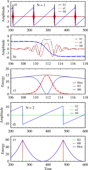
Figure 1: Weak forcing $f=0.1$: (a) Amplitudes $b_{0},a_{1},b_{1}$ for $N=1$, intervals $\approx 110$, (b) amplitudes during a flow reversal with Eq. (33) for $b_{0}$ (dashed), (c) energies $H_{0},H_{1}$ and Eq. (34) for $H_{1}$ (dashed), (d) amplitudes $b_{0},a_{2},b_{2}$ for $N=2$, ($a_{1},b_{1}$ vanish), and (e) energies ($H_{1}$ vanishes).

The mean flow is $U=b_{0}$ which is subject to a constant forcing $f$ in the numerical experiments (24). The truncated system conserves energy

$$H_{tot}=H_{0}+H_{1}+H_{2}$$ (29)

$$H_{0}=\frac{1}{2}b_{0}^{2},\quad H_{1}=\frac{1}{4}\left(a_{1}^{2}+b_{1}^{2}\right),\quad H_{2}=\frac{1}{4}\left(a_{2}^{2}+b_{2}^{2}\right)$$ (30)

The Liouville Theorem is not satisfied

$$\sum_{n=0}^{2}\left(\frac{\partial\dot{a}_{n}}{\partial a_{n}}+\frac{\partial\dot{b}_{n}}{\partial b_{n}}\right)=\frac{5}{3}b_{0}$$ (31)

The expansion and contraction of the state space volume is controlled by the sign of the mean flow.

Numerical experiments reveal a flow reversal mechanism and vanishing long term means of mean flow and wave number amplitudes, hence the Liouville Theorem (31) is satisfied in the mean.

(i) Weak forcing with $f=0.1$ in the $N=1$ truncation reveals periodic flow reversals (Fig. 1). The system starts with randomly chosen amplitudes. A mean flow increases gradually to positive values where it becomes unstable due to the excited waves, denoted as breathers in the following. These breathers drive a rapid flow reversal towards a negative flow which initiates their collapse. The process is energy conserving on short time scales. The total energy increases (decreases) when the mean flow is positive (negative).

For $N=1$ with the amplitudes $b_{0},a_{1},b_{1}$ the energy cycle is for $f=0$ (compare (20, 22))

$$\partial_{t}H_{0}=-\frac{1}{3}b_{0}H_{1},\qquad\partial_{t}H_{1}=\frac{1}{3}b_{0}H_{1}$$ (32)

which is controlled by the mean flow. The solution for the mean flow is for $b_{0}(0)=0$

$$b_{0}=-6a\tanh(at)$$ (33)

and the perturbation energy is

$$H_{1}=\frac{18a^{2}}{\cosh^{2}(at)}$$ (34)

where $a$ is related to the total energy $H=18a^{2}$. $H_{1}$ attains its maximum during flow reversals when $U=0$. These approximations are compared to the forced simulation in Fig. 1b,c centered at a single flow reversal.

In the presence of forcing $f$ and for a small wave energy $H_{1}$ the mean flow $b_{0}$ grows linearly in time, $b_{0}(t)\approx ft$, up to a value $b_{0,max}$. This defines an interarrival time scale of flow reversals, $\tau=2b_{0,max}/f$. In this range the wave energy evolves rapidly according to $H_{1}(t)\sim\exp(ft^{2}/6)$.

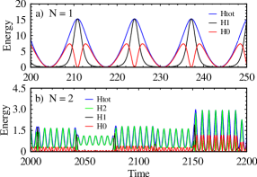
Figure 2: Intermediate forcing $f=1$: Energy distributions for (a) $N=1$, intervals $\approx 13$, (b) $N=2$.

The described flow reversal mechanism is retained for viscous dissipation represented by a linear damping of the wave amplitudes $a_{1}$ and $b_{1}$.

For the $N=2$ truncation with all modes $b_{0},a_{1},b_{1},a_{2}$ and $b_{2}$ flow reversals occur on a time scale roughly twice as for $N=1$ (Fig. 1d). Due to the weak forcing the energy cascades to mode 2 with negligible amplitudes $a_{1},b_{1}$ and energy $H_{1}$ (Fig. 1d, e). Neglecting the modes 1, the energy cycle for interactions among $b_{0},a_{2}$ and $b_{2}$ is

$$\partial_{t}H_{0}=-\frac{4}{3}b_{0}H_{2},\qquad\partial_{t}H_{2}=\frac{4}{3}b_{0}H_{2}$$ (35)

This corresponds to a rescaling of the $H_{0}-H_{1}$ cycle (32) by $\tilde{t}=2t$ for time and $\tilde{b}_{0}=2b_{0}$ etc. for the amplitudes, hence the energies quadruple.

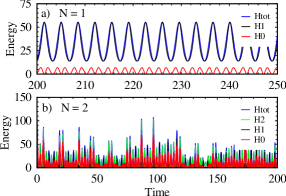
Figure 3: Strong forcing $f=10$: energy distributions for (a) $N=1$, intervals $\approx 3$, (b) $N=2$.

(ii) For intermediate forcing with $f=1$ the time scale between flow reversals decreases by an order of magnitude in the $N=1$ truncation (see Fig. 2a). Thus the intervals $\tau$ approach the duration of individual breathers. For the complete set of modes in $N=2$ (Fig. 2b) the system is weakly nonlinear with a mixing of frequencies, $\omega/2,\omega,3\omega/2$ and $2\omega$, where $\omega=2\pi/\tau$ is defined by the interarrival times of the flow reversals Lucarini and Fraedrich (2009). The lowest frequency determines the amplitude modulation.

(iii) For strong forcing, $f=10$, the flow reversals in the $N=1$ truncation are regular (Fig. 3a) with intervals decreased by an order of magnitude relative to $f=1$. The dominant part of energy is accumulated in waves. In the $N=2$ truncation the dynamics becomes intermittent as in the regime behaviour detected by Lorenz Lorenz (2006) in the discrete equations (1). The events loose their identities and the systen becomes strongly nonlinear.

In Summary, a continuous dynamical equation derived from the Lorenz-96 model is able to mimic several types of complex processes observed in geophysics, geophysical fluid dynamics, and solid state physics:

(i) Avalanche processes excited by continuous driving as in the sand pile model of Bak et al. Bak et al. (1987); see also the recent observation of quasi-periodic events in crystal plasticity subject to external stress Papanikolaou et al. (2012). A common characteristic property is the weakness of the external forcing which is necessary to cause avalanches. In the present model the flow is driven by a constant forcig towards a state where mean flow and wave energy interact. The intervals between the flow reversals are approximately proportional to the inverse of the forcing intensity, $\sim 1/f$.

(ii) The Quasi-Biennial Oscillation (QBO, Baldwin et al. (2001)), a flow reversal in the tropical stratosphere driven by two different types of upward propagating gravity waves. A common aspect is that the driving of the mean flow by waves occurs only for a particular sign of the mean flow. Although the QBO is considered to be explained dynamically the simulation in present-day weather and climate models necessitates careful sub-scale parameterizations or high resolution models Kawatani et al. (2010). The present model is clearly an oversimplification but can be considered as a toy model for this phenomenon.

(iii) Rogue waves (also termed freak or monster waves) at the ocean surface are simulated mainly by the nonlinear Schroedinger equation (e.g. Onorato et al. (2006); Calini and Schober (2012)); a Lagrangian analysis has been published recently Abrashkin and Soloviev (2013). The breather solutions found in the present model show characteristics like the rapid evolution and the high intensity in an almost quiescent medium.

Due to the flow reversals the total energy of the non-dissipative system remains finite for a constant forcing. The long term mean of the mean flow vanishes and the Liouville Theorem (31) is satisfied in the mean. The flow reversals are insensitive to viscous dissipation.