Factorization in high energy nucleus-nucleus collisions

Abstract

In this talk, we discuss the factorization of the logarithms of energy in the Color Glass Condensate framework.

11.10.-z, 11.15.-q, 11.80.La, 11.15.Kc

1 Color Glass Condensate

Heavy ion collisions at high energy are a situation in which the colliding projectiles contain high densities of gluons, and are possibly subject to the phenomenon of gluon saturation [1, 2, 3]: when the gluon occupation number approaches the inverse of the strong coupling constant $\alpha_{s}$, the interactions among the gluons become strong, and non-linear effects such as recombination become important.

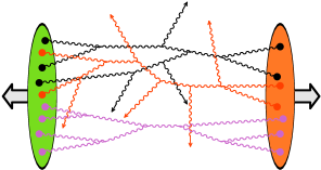
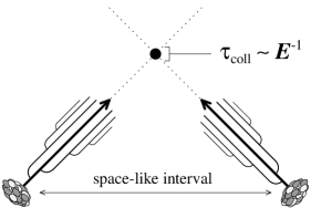
Figure 1: Left: typical graphs in the collision of two saturated projectiles. Right: Causality argument underlying factorization.

Moreover, in this regime a typical collision involves multiple gluon interactions, as depicted in the figure 1 (left). Unlike in the dilute regime, multiple gluons from each projectile can participate in the reaction. This leads to two complications: we a way to organize and resum all the relevant graphs, and we need multi-gluon distributions to describe the projectiles. Both are provided by the Color Glass Condensate effective theory [4, 5, 6], in which the incoming nuclei are described as collections of color charges moving at the speed of light along the light-cones.

The object that encodes this information is a probability distribution $W[\rho]$, where $\rho({\boldsymbol{x}}_{\perp})$ is the color charge per unit of transverse area of a given nucleus. In the saturated regime, this density is inversely proportional to the coupling, and observables at leading order are obtained by summing an infinite series of tree diagrams, which can be done more conveniently by solving the classical Yang-Mills equations, in which the charge density $\rho$ plays the role of a source term.

Next-to-leading order corrections are made of one-loop diagrams in a classical background field. When computing NLO corrections, the CGC should be viewed as an effective theory with an upper cutoff $\Lambda$ on the longitudinal momentum running in the loop (see the figure 2, left), in order to prevent double counting the modes already taken into account via the source $\rho$. NLO corrections in general contain logarithms of this unphysical cutoff. For the CGC framework to be consistent, observables should be cutoff independent in the end. For a given observable, it is possible to make the distribution $W[\rho]$ cutoff dependent in order to cancel the cutoff dependence coming from the loop correction. However, for this strategy to be useful in practice, two requirements should be satisfied :

• the same $W[\rho]$ should be able to cancel the cutoff dependence of a wide range of observables,

• when colliding two such projectiles, each of them should have its own $W[\rho]$. Moreover, these distributions should be the same as in simpler collisions such as Deep Inelastic Scattering (DIS), that involve only one saturated projectile.

Under these conditions, the distribution $W[\rho]$ can be viewed as an intrinsic property of a saturated projectile, and its cutoff dependence reflects changes in its apparent color content due to a change in the resolution scale.

2 Factorization in Deep Inelastic Scattering

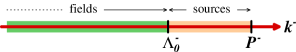
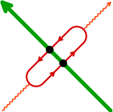
Figure 2: Left: separation between sources and fields in the CGC effective theory. Right: DIS reaction at leading order.

Let us start with a reminder of the situation in inclusive DIS off a dense nucleus. Thanks to the optical theorem, the total DIS cross-section is related to the forward elastic scattering amplitude of the virtual photon on the nucleus, and at LO it corresponds to the scattering of a quark-antiquark fluctuation of the photon off the classical color field ${\cal A}^{\mu}$ of the nucleus (see the figure 2, right) :

$${{\boldsymbol{T}}_{{}_{\rm LO}}(\vec{\boldsymbol{x}}_{\perp},\vec{\boldsymbol{y}}_{\perp})} = 1-\frac{1}{N_{c}}\,{\rm tr}\,({{U(\vec{\boldsymbol{x}}_{\perp})U^{\dagger}(\vec{\boldsymbol{y}}_{\perp})}})$$

$$U(\vec{\boldsymbol{x}}_{\perp}) = {\rm P}\,\exp\,i{g}\int^{1/xP^{-}}\!\!\!\!\!\!dz^{+}\,{{\cal A}^{-}(z^{+},\vec{\boldsymbol{x}}_{\perp})}\;.$$ (1)

Note that the $q\bar{q}$ pair couples only to the sources up to the longitudinal coordinate $z^{+}\lesssim(xP^{-})^{-1}$. The other sources are too slow to be seen by the dipole.

At NLO, one needs corrections involving a gluon, such as the one in the right of the figure 3. The longitudinal momentum of this gluon should be integrated only up to the cutoff $\Lambda_{0}^{-}$ of the CGC effective theory. In practice, it is more convenient to include only longitudinal modes in a slice $\Lambda_{1}^{-}<k^{-}<\Lambda_{0}^{-}$.

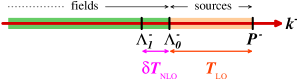
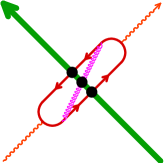
Figure 3: Left: small shift of the cutoff scale. Right: DIS reaction at next to leading order.

At leading log accuracy, the contribution of the quantum modes in that strip is :

$${\delta{\boldsymbol{T}}_{{}_{\rm NLO}}(\vec{\boldsymbol{x}}_{\perp},\vec{\boldsymbol{y}}_{\perp})}=\ln\left(\frac{\Lambda_{0}^{-}}{\Lambda_{1}^{-}}\right)\;{{\cal H}}\;{{\boldsymbol{T}}_{{}_{\rm LO}}(\vec{\boldsymbol{x}}_{\perp},\vec{\boldsymbol{y}}_{\perp})}\;,$$ (2)

where ${\cal H}$ is an operator that contains functional derivatives with respect to the source $\rho$, called the JIMWLK Hamiltonian. These NLO corrections can be absorbed in the LO result,

$$\Big{<}{{\boldsymbol{T}}_{{}_{\rm LO}}}+{\delta{\boldsymbol{T}}_{{}_{\rm NLO}}}\Big{>}_{\Lambda_{0}^{-}}=\Big{<}{{\boldsymbol{T}}_{{}_{\rm LO}}}\Big{>}_{\Lambda_{1}^{-}}\;,\quad\big{<}\cdots\big{>}_{{}_{\Lambda}}\equiv\int[D\rho]\,W_{\Lambda}[\rho]\,\cdots$$ (3)

provided one defines a new effective theory with a lower cutoff $\Lambda_{1}^{-}$ and a modified distribution of sources $W_{\Lambda_{1}^{-}}[\rho]$ :

$$W_{\Lambda_{1}^{-}}\equiv\Big{[}1+\ln\left(\frac{\Lambda_{0}^{-}}{\Lambda_{1}^{-}}\right)\;{{\cal H}}\Big{]}\;W_{\Lambda_{0}^{-}}\;,\quad\mbox{i.e.}\quad\frac{\partial W_{\Lambda}}{\partial\ln(\Lambda)}=-{\cal H}\,W_{\Lambda}\;.$$ (4)

By solving this equation (known as the JIMWLK equation) until the cutoff has been lowered to the value $xP^{-}$, one can sequentially resum the leading log contributions from each of the $k^{-}$ slices below the original cutoff.

3 Factorization in nucleus-nucleus collisions

In high energy nucleus-nucleus collisions, there are now two saturated projectiles, and it is more difficult to extract the logarithms that arise in observables at NLO. There is however a simple argument explaining qualitatively the universality of the distributions $W[\rho]$ that describe these projectiles in the CGC framework, illustrated in the figure 1 (right). The soft gluon radiation responsible for the logarithms of the cutoff takes a long time, much shorter than the collision time that goes like the inverse of the collision energy. Therefore, these gluons must be emitted before the collision, at a time where the separation between the projectiles is space-like. For this reason, there cannot be any cross-talk between the distributions $W[\rho]$ that describe the two nuclei, and they should be the same as in DIS.

In order to illustrate how this works in an actual calculation, let us consider the inclusive gluon spectrum at LO and NLO, illustrated in the two diagrams on the left of the figure 4.

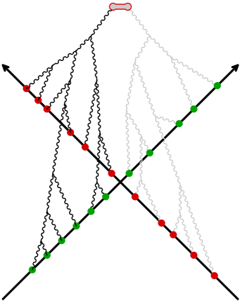
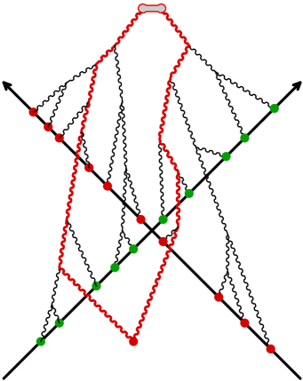
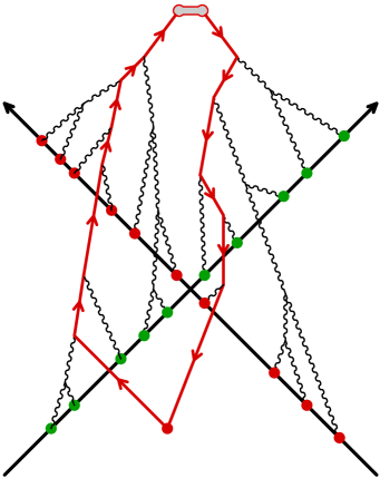
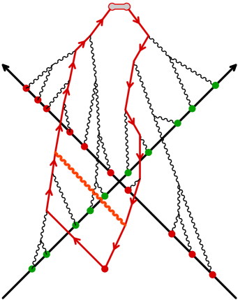
Figure 4: Left: inclusive gluon spectrum at LO and NLO. Right: inclusive quark spectrum at LO and NLO.

At LO, the gluon spectrum is quadratic in the retarded solution of the classical Yang-Mills equation,

$$\left.\frac{dN_{g}}{dyd^{2}\vec{\boldsymbol{p}}_{\perp}}\right|_{{}_{\rm LO}}\propto\int d^{4}xd^{4}y\;e^{ip\cdot(x-y)}\cdots{{\cal A}^{\mu}(x){\cal A}^{\nu}(y)}\;,$$ (5)

$$\quad{\big{[}{{\cal D}_{\mu}},{{\cal F}^{\mu\nu}}\big{]}={J_{1}^{\nu}}+{J_{2}^{\nu}}}\quad,\quad\lim_{t\to-\infty}{{\cal A}^{\mu}(t,\vec{\boldsymbol{x}})}=0\;.$$ (6)

At NLO, it involves one-loop graphs in the presence of a background color field. One can formally express the NLO result as[7]

$$\left.{\frac{dN_{g}}{dyd^{2}\vec{\boldsymbol{p}}_{\perp}}}\right|_{{}_{\rm NLO}}=\Bigg{[}\frac{1}{2}\!\!\!\!\int\limits_{{}_{\vec{\boldsymbol{u}},\vec{\boldsymbol{v}}\in\Sigma}}\!\!\!\!\int_{\boldsymbol{k}}\big{[}{a_{\boldsymbol{k}}}\,{\mathbbm{T}}\big{]}_{\boldsymbol{u}}\big{[}{a_{\boldsymbol{k}}^{*}}\,{\mathbbm{T}}\big{]}_{\boldsymbol{v}}+\int\limits_{{}_{\vec{\boldsymbol{u}}\in\Sigma}}\big{[}{{\boldsymbol{\alpha}}}\,{\mathbbm{T}}\big{]}_{\boldsymbol{u}}\Bigg{]}\;\left.{\frac{dN_{g}}{dyd^{2}\vec{\boldsymbol{p}}_{\perp}}}\right|_{{}_{\rm LO}}\;,$$ (7)

where ${\boldsymbol{\alpha}}$ and $a_{\boldsymbol{k}}$ are small perturbations to the classical field ${\cal A}$, $\Sigma$ a surface used to set the initial condition for the fields (e.g. the light-cone), and ${\mathbbm{T}}_{\boldsymbol{u}}$ the functional derivative with respect to the initial classical field at the point ${\boldsymbol{u}}\in\Sigma$. In this formula, the integration over ${\boldsymbol{k}}$ has a logarithmic dependence on the cutoff

$$\frac{1}{2}\!\!\!\!\int\limits_{{}_{\vec{\boldsymbol{u}},\vec{\boldsymbol{v}}\in\Sigma}}\!\!\!\!\int_{\boldsymbol{k}}\big{[}{a_{\boldsymbol{k}}}\,{\mathbbm{T}}\big{]}_{\boldsymbol{u}}\big{[}{a_{\boldsymbol{k}}^{*}}\,{\mathbbm{T}}\big{]}_{\boldsymbol{v}}+\int\limits_{{}_{\vec{\boldsymbol{u}}\in\Sigma}}\big{[}{{\boldsymbol{\alpha}}}\,{\mathbbm{T}}\big{]}_{\boldsymbol{u}}=\ln\left(\Lambda^{+}\right)\,{{\cal H}_{1}}+\ln\left(\Lambda^{-}\right)\,{{\cal H}_{2}}+\cdots$$ (8)

where ${\cal H}_{1,2}$ are the JIMWLK Hamiltonians of the two nuclei. This formula is the formal realization of the causality argument exposed at the beginning of this section, since the logarithms associated to the two cutoffs are accompanied by the JIMWLK of the corresponding nucleus, without any mixing. Thanks to this formula, one can absorb the logarithms of the cutoff in JIMWLK-evolved distributions of color sources,

$$\left<\frac{dN_{g}}{dyd^{2}\vec{\boldsymbol{p}}_{\perp}}\right>_{{}_{\rm LeadingLog}}=\int\big{[}D{\rho_{{}_{1}}}\,D{\rho_{{}_{2}}}\big{]}\;{W_{1}\big{[}\rho_{{}_{1}}\big{]}}\;{W_{2}\big{[}\rho_{{}_{2}}\big{]}}\;{\frac{dN_{g}[\rho_{1,2}]}{dyd^{2}\vec{\boldsymbol{p}}_{\perp}}}\;.$$ (9)

The same factorization holds for multi-gluon inclusive spectra[8, 9], and more generally for all the inclusive observables, for which eq. (7) is valid.

4 Extension to quark production (work in progress)

A natural extension of these results is to study it in the case of quark production. To that effect, one needs expressions for the quark spectrum at LO and NLO (see the two diagrams on the right of the figure 4). These contributions have been worked out, and it turns out that they are related by a formula similar to eq. (7)[10],

$$\left.{\frac{dN_{{}_{Q}}}{dyd^{2}\vec{\boldsymbol{p}}_{\perp}}}\right|_{{}_{\rm NLO}}=\smash{\Bigg{[}\frac{1}{2}\!\!\!\!\int\limits_{{}_{\vec{\boldsymbol{u}},\vec{\boldsymbol{v}}\in\Sigma}}\!\!\!\!\int_{\boldsymbol{k}}\big{[}{a_{\boldsymbol{k}}}\,{\mathbbm{T}}+\underline{{b_{\boldsymbol{k}}}\,{\mathbbm{T}}_{{}_{\psi}}}\big{]}_{\boldsymbol{u}}\big{[}{a_{\boldsymbol{k}}^{*}}\,{\mathbbm{T}}+\underline{{b_{\boldsymbol{k}}^{\dagger}}\,{\mathbbm{T}}_{{}_{\psi}}}\big{]}_{\boldsymbol{v}}}$$

$$\qquad\qquad\qquad\qquad\quad{+\int\limits_{{}_{\vec{\boldsymbol{u}}\in\Sigma}}\big{[}{{\boldsymbol{\alpha}}}\,{\mathbbm{T}}+\underline{{{\boldsymbol{\beta}}}\,{\mathbbm{T}}_{{}_{\psi}}}\big{]}_{\boldsymbol{u}}\Bigg{]}\;\left.{\frac{dN_{{}_{Q}}}{dyd^{2}\vec{\boldsymbol{p}}_{\perp}}}\right|_{{}_{\rm LO}}}\;,$$ (10)

where the underlined terms are new and contain purely fermionic quantities : $b_{\boldsymbol{k}}$ and ${\boldsymbol{\beta}}$ are small fermionic fields, and where the operator ${\mathbbm{T}}_{\psi}$ is a functional derivative with respect to the initial value of fermion fields on $\Sigma$. This formula is only the first step; the second part of this program consists in extracting the logarithms from the new fermionic terms in the operator that appears in the right hand side, and to prove that they are also proportional to the JIMWLK Hamiltonian.

References

- [1] L.V. Gribov, E.M. Levin, M.G. Ryskin, Phys. Rept. 100, 1 (1983).
- [2] A.H. Mueller, J-W. Qiu, Nucl. Phys. B 268, 427 (1986).
- [3] T. Lappi, Int. J. Mod. Phys. E20, 1 (2011).
- [4] E. Iancu, A. Leonidov, L.D. McLerran, Lectures given at Cargese Summer School on QCD Perspectives on Hot and Dense Matter, Cargese, France, 6-18 Aug 2001, hep-ph/0202270.
- [5] E. Iancu, R. Venugopalan, Quark Gluon Plasma 3, Eds. R.C. Hwa and X.N. Wang, World Scientific, hep-ph/0303204.
- [6] F. Gelis, E. Iancu, J. Jalilian-Marian, R. Venugopalan, Ann. Rev. Part. Nucl. Sci. 60, 463 (2010).
- [7] F. Gelis, T. Lappi, R. Venugopalan, Phys. Rev. D 78, 054019 (2008).
- [8] F. Gelis, T. Lappi, R. Venugopalan, Phys. Rev. D 78, 054020 (2008).
- [9] F. Gelis, T. Lappi, R. Venugopalan, Phys. Rev. D 79, 094017 (2009).
- [10] F. Gelis, J. Laidet, arXiv:1211.1191 [hep-ph].