Generalized Householder Transformations
for the Complex Symmetric Eigenvalue Problem

Abstract

We present an intuitive and scalable algorithm for the diagonalization of complex symmetric matrices, which arise from the projection of pseudo–Hermitian and complex scaled Hamiltonians onto a suitable basis set of “trial” states. The algorithm diagonalizes complex and symmetric (non–Hermitian) matrices and is easily implemented in modern computer languages. It is based on generalized Householder transformations and relies on iterative similarity transformations $\bm{T}\to\bm{T}^{\prime}=\bm{Q}^{\rm T}\,\bm{T}\,\bm{Q}$, where $\bm{Q}$ is a complex and orthogonal, but not unitary, matrix, i.e, $\bm{Q}^{\rm T}=\bm{Q}^{-1}$ but $\bm{Q}^{\mbox{{\bf{\tiny+}}}}\neq\bm{Q}^{-1}$. We present numerical reference data to support the scalability of the algorithm. We construct the generalized Householder transformations from the notion that the conserved scalar product of eigenstates $\Psi_{n}$ and $\Psi_{m}$ of a pseudo–Hermitian quantum mechanical Hamiltonian can be reformulated in terms of the generalized indefinite inner product $\int\mathrm{d}x\,\Psi_{n}(x,t)\,\Psi_{m}(x,t)$, where the integrand is locally defined, and complex conjugation is avoided. A few example calculations are described which illustrate the physical origin of the ideas used in the construction of the algorithm.

I Introduction

Complex symmetric matrices $\bm{A}=\bm{A}^{\rm T}$ arise naturally from the projection of a complex scaled (“‘resonance-generating”) Hamiltonian onto a basis of quantum mechanical “trial” states. For suitably chosen parameters, the diagonalization of a matrix of this type leads to (accurate) approximations for the resonance energies, and the resonance eigenstates, of the complex scaled Hamiltonian JeSuLuZJ2008 ; JeSuZJ2009prl ; JeSuZJ2010 ; ZJJe2010jpa . The resonance energies are manifestly complex; the width of the quantum state enters the complex energy as $E=\mathrm{Re}\,E-\frac{\mathrm{i}}{2}\Gamma$, where $\Gamma$ is the width (we use natural units with $\hbar=c=\epsilon_{0}=1$ throughout this article). A paradigmatic example JeSuLuZJ2008 is the complex-scaled cubic anharmonic oscillator Hamiltonian $h_{3}=-\frac{1}{2}\,\exp(-2\mathrm{i}\theta)\,\partial_{x}^{2}+\frac{1}{2}\,\exp(2\mathrm{i}\theta)\,x^{2}+G\,\exp(3\mathrm{i}\theta)\,x^{3}$, where $G$ is a coupling parameter and $0<\theta<\pi/5$ is a complex rotation angle.

However, complex scaled Hamiltonians are not the only source of complex symmetric matrices in theoretical physics. For example, if one projects the pseudo–Hermitian ($\mathcal{PT}$-symmetric) anharmonic oscillator BeBo1998 ; BeBoMe1999 Hamiltonian $H_{3}=-\frac{1}{2}\,\partial_{x}^{2}+\frac{1}{2}\,x^{2}+\mathrm{i}\,G\,x^{3}$ with an imaginary cubic perturbation ($G>0$) onto a basis of harmonic oscillator eigenstates, then one obtains a complex symmetric (but not Hermitian) matrix, the eigenvalues of which are real.

As shown in Refs. JeSuZJ2009prl ; BeDu1999 , the complex resonance energies of the “real” cubic anharmonic oscillator $h_{3}$ are connected with the real eigenenergies of the imaginary cubic perturbation $H_{3}$ via a dispersion relation. The same holds true for all anharmonic oscillators of odd degree. Some of the numerical calculations were instrumental in providing additional evidence for the generalization JeSuZJ2009prl of the so-called Bender–Wu formulas BeWu1969 ; BeWu1971 , which describe the large-order asymptotic growth of the perturbative coefficients of an arbitrary energy eigenvalue of an even anharmonic oscillator, to odd anharmonic oscillators. Indeed, the conjectures on nonperturbative quantization conditions, described in Refs. JeSuZJ2009prl ; JeSuZJ2010 had been checked against high-precision numerical data before the results were presented.

The purpose of this paper is threefold: First, to illustrate the numerical procedures underlying the numerical verification of the conjectured generalized quantization conditions, second, to describe an intuitive and scalable (in terms of the numerical precision) matrix diagonalization algorithm which seems to be particularly suited for the treatment of complex symmetric matrices. Our algorithm has a certain “twist” in the sense that it is based on generalized Householder transformations. The generalized Householder matrices ${\bm{H}}_{\bm{v}}$ have manifestly complex entries but are not Hermitian unlike the familiar formalism (see p. 225 of Ref. StBu2002 ). Instead, they are orthogonal matrices with the property ${\bm{H}}_{\bm{v}}\,{\bm{H}}^{\rm T}_{\bm{v}}=\mathbbm{1}$. To the best of our knowledge, these generalized Householder reflections have not appeared in the standard literature Wi1965 ; WiRe1971 ; GovL1996 ; Pa1998matrix ; AnEtAl1999 on matrix diagonalization procedures before.

Finally, the third purpose of the paper is to illustrate a few properties of the eigenenergies of pseudo–Hermitian Hamiltonians, based on calculations done with the algorithm presented here. Let us anticipate one of the observations made in the course of the calculations. At face value, the conserved scalar product BeBrReRe2004 (under the time evolution governed by a pseudo–Hermitian anharmonic oscillator) is given as the integral $\int\mathrm{d}x\,\Psi_{n}^{*}(-x,t)\,\Psi_{m}(x,t)$; this expression involves a non-local integrand with function evaluations at $x$ and $-x$. Typically, eigenstates of complex symmetric matrices are orthogonal with regard to a conceptually much simpler scalar product, namely, the indefinite inner product $\int\mathrm{d}x\,\Psi_{n}(x,t)\,\Psi_{m}(x,t)$, where the integrand is locally defined, and complex conjugation is avoided. However, the two scalar products are related, as described in this article, and this observation has motivated the construction of the matrix diagonalization algorithm presented here. We thus proceed by describing the algorithm in Sec. II and the physical motivation for its development in Sec. III, together with a few example calculations. Conclusions are reserved for Sec. IV.

II Complex Symmetric Eigenvalues and Eigenvectors

II.1 Orientation

Quantum mechanics is formulated in an infinite-dimensional vector space (Hilbert space) of functions. However, once a numerical evaluation of eigenvalues of a particular Hamiltonian is pursued, the quantum mechanical Hamiltonian needs to be projected onto a suitable basis set of wave functions, leading to a finite-dimensional matrix.

When a pseudo-Hermitian Hamiltonian such as the imaginary cubic oscillator is projected onto a basis set consisting of harmonic-oscillator eigenfunction, one obtains a complex symmetric (not Hermitian!) matrix. Typically, the generalized indefinite inner product GoLaRo1983 ; Mo1998 ; ArHo2004 naturally emerges as a tool in the analysis of pseudo–Hermitian quantum mechanics, and one would thus naturally assume that the indefinite inner product might be useful in the development of a suitable matrix diagonalization algorithm. Indeed, the approximate calculation of eigenvalues of quantum mechanical Hamiltonians naturally emerges as a task in the analysis of the quantum dynamics induced by the pseudo–Hermitian time evolution.

Such an algorithm will be described in the following; it essentially relies on two steps: In the first, the complex symmetric input matrix is transformed to tridiagonal form, and in the second step, the tridiagonal matrix is diagonalized to machine accuracy. The first step uses the concept of the complex inner product in an absolutely essential manner; it is based on generalized Householder reflection matrices. The complex symmetric input matrix is transformed to tridiagonal form in a single computation whose computational cost is of order $n^{2}$ (here, “tridiagonal form” refers to a form where the diagonal, as well as the sub- and superdiagonal entries of the matrix are nonzero). For the second step, one has a number of methods available; we shall briefly outline a method based on an iterative QL decompositions with an implicit (Wilkinson) shift.

II.2 Tridiagonalization

We first define the indefinite inner product for finite-dimensional $n$-vectors as follows,

$$\langle{\bm{x}},{\bm{y}}\rangle_{*}=\sum_{i=1}^{n}x_{i}\,y_{i}={\bm{x}}^{{\rm T}}\cdot{\bm{y}}\,,$$ (1)

where ${\bm{x}}^{{\rm T}}$ is a row vector, whereas ${\bm{y}}$ is a column vector. Note that the entries of ${\bm{x}}$ and ${\bm{y}}$ may be complex numbers, but complex conjugation of either ${\bm{x}}$ or ${\bm{y}}$ is avoided. We use generalized Householder reflection matrices ${\bm{H}}_{\bm{v}}$, which have the properties,

$${\bm{H}}_{\bm{v}}= \;\mathbbm{1}-\frac{2}{\langle{\bm{v}},{\bm{v}}\rangle_{*}}\,{\bm{v}}\otimes{\bm{v}}^{{\rm T}}\,,\qquad{\bm{H}}_{\bm{v}}\;{\bm{x}}={\bm{x}}-2{\bm{u}}\left<{\bm{u}},{\bm{x}}\right>_{*}\,,\qquad{\bm{u}}=\frac{{\bm{v}}}{|{\bm{v}}|_{*}}\,,\qquad|{\bm{v}}|_{*}=\sqrt{\langle{\bm{v}},{\bm{v}}\rangle_{*}}\,.$$ (2)

Here, the dyadic product of a column and a row vector is denoted by the symbol $\otimes$, and the branch cut of the square root function in the calculation of $|{\bm{v}}|_{*}$ is along the negative real axis.

The generalized Householder reflection matrix ${\bm{H}}_{{\bm{v}}}$ is symmetric, i.e., ${\bm{H}}_{\bm{v}}={\bm{H}}_{\bm{v}}^{\rm T}$. Furthermore, the Householder reflections are square roots of the unit matrix,

$${\bm{H}}_{\bm{v}}^{2}= \;{\bm{H}}_{\bm{v}}\;{\bm{H}}_{\bm{v}}^{\rm T}={\bm{H}}_{\bm{v}}^{\rm T}\;{\bm{H}}_{\bm{v}}=\mathbbm{1}-4{\bm{u}}\otimes{\bm{u}}^{T}+4\,{\bm{u}}\otimes{\bm{u}}^{T}\;\left<{\bm{u}},{\bm{u}}\right>_{*}=\mathbbm{1}.$$ (3)

A characteristic property of the Householder reflections is that the parameter vector ${\bm{v}}$ can be adjusted so that the input vector ${\bm{x}}$ is projected onto a particular axis, upon the calculation of ${\bm{H}}_{\bm{v}}\;{\bm{y}}$. We set

$${\bm{v}}={\bm{y}}+|{\bm{y}}|_{*}\;{\hat{\bm{e}}}_{n}\,,$$ (4)

where $\hat{\bm{e}}_{n}$ is the “last” unit vector in the $n$-dimensional space, and we verify that

$${\bm{H}}_{\bm{v}}\;{\bm{y}}= \;{\bm{y}}-\frac{2}{\left<{\bm{v}},{\bm{v}}\right>_{*}}\,\left<{\bm{v}},{\bm{y}}\right>_{*}\,{\bm{v}}={\bm{y}}-\frac{2\left({\bm{y}}^{\rm T}+|{\bm{y}}|_{*}\;\hat{\bm{e}}^{\rm T}_{n}\right)\cdot{\bm{y}}}{\left({\bm{y}}^{\rm T}+|{\bm{y}}|_{*}\,\hat{\bm{e}}^{T}_{n}\right)\cdot\left({\bm{y}}+|{\bm{y}}|_{*}\hat{\bm{e}}_{n}\right)}{\bm{v}}$$

$$= \;{\bm{y}}-\frac{2\left(|{\bm{y}}|_{*}^{2}+|{\bm{y}}|_{*}y_{n}\right)}{2|{\bm{y}}|_{*}^{2}+2|{\bm{y}}|_{*}y_{n}}{\bm{v}}={\bm{y}}-{\bm{v}}=-|{\bm{y}}|_{*}\hat{\bm{e}}_{n}\,.$$ (5)

Furthermore,

$${\bm{y}}^{\rm T}{\bm{H}}_{\bm{v}}=({\bm{H}}_{\bm{v}}{\bm{y}})^{\rm T}=-|{\bm{y}}|_{*}\hat{\bm{e}}_{n}^{\rm T}\;.$$ (6)

The results from Eqs. (5) and (6) are useful in the tridiagonalization procedure. Let ${\bm{A}}$ be the matrix we want to tridiagonalize. In the first step, we choose the column vector ${\bm{y}}_{n-1}$ to consist of the first $n-1$ elements of the last column of ${\bm{A}}$,

$${\bm{y}}_{n-1}=\left(\begin{array}[]{c}A_{1\,n}\\ A_{2\,n}\\ \vdots\\ A_{n-1\,n}\end{array}\right).$$ (7)

By defining ${\bm{B}}_{n-1}$ as an $(n-1)\times(n-1)$ matrix where $B_{ij}=A_{ij}$, for $i,j=1,\dots,n-1$, we can write ${\bm{A}}$ as

$${\bm{A}}=\left(\begin{array}[]{ccc|c}&&&\\ &{\bm{B}}_{n-1}&&{\bm{y}}_{n-1}\\ &&&\\ \hline\cr&\rule[-8.53581pt]{0.0pt}{22.76219pt}{\bm{y}}_{n-1}^{\rm T}&&A_{nn}\end{array}\right)\,.$$ (8)

In the spirit of the Householder reflection, we set

$${\bm{v}}_{n-1}={\bm{y}}_{n-1}+|{\bm{y}}_{n-1}|_{*}\,\hat{\bm{e}}_{n-1}\,.$$ (9)

We can then construct ${\bm{H}}_{{\bm{v}}_{n-1}}$, which will be a Householder matrix of rank $n-1$. The complex $n\times n$ matrix ${\bm{H}}_{n-1}$ is defined as

$${\bm{H}}_{n-1}=\left(\begin{array}[]{ccc|c}&&&\\ &{\bm{H}}_{{\bm{v}}_{n-1}}&&\vec{0}\\ &&&\\ \hline\cr&\rule[-8.53581pt]{0.0pt}{22.76219pt}\vec{0}^{\rm T}&&1\end{array}\right)\,.$$ (10)

Then,

$${\bm{A}}^{\prime} ={\bm{H}}_{n-1}\;{\bm{A}}\;{\bm{H}}_{n-1}=\left(\begin{array}[]{ccc|c}&&&\\ &{\bm{H}}_{{\bm{v}}_{n-1}}{\bm{B}}_{n-1}{\bm{H}}_{{\bm{v}}_{n-1}}&&{\bm{H}}_{{\bm{v}}_{n-1}}{\bm{y}}_{n-1}\\ &&&\\ \hline\cr&{\bm{y}}_{n-1}^{\rm T}{\bm{H}}_{{\bm{v}}_{n-1}}&&A_{nn}\end{array}\right).$$ (15)

Using Eq. (5) and (6), this can be reduced to

$${\bm{A}}^{\prime}=\left(\begin{array}[]{ccc|c}&&&0\\ &{\bm{B}}^{\prime}_{n-1}&&\vdots\\ &&&-|{\bm{y}}_{n-1}|_{*}\\ \hline\cr 0&\cdots&-|{\bm{y}}_{n-1}|_{*}&A_{nn}\end{array}\right),$$ (16)

where

$${\bm{B}}^{\prime}_{n-1}={\bm{H}}_{{\bm{v}}_{n-1}}{\bm{B}}_{n-1}{\bm{H}}_{{\bm{v}}_{n-1}}\,.$$ (17)

For the second step we choose ${\bm{y}}_{n-2}$ to be the first $n-2$ elements of the second to last column of ${\bm{A}}^{\prime}$,

$${\bm{y}}_{n-2}=\left(\begin{array}[]{c}A^{\prime}_{1\,n-1}\\ A^{\prime}_{2\,n-1}\\ \vdots\\ A^{\prime}_{n-2\,n-1}\end{array}\right)\,,\quad{\bm{v}}_{n-2}={\bm{y}}_{n-2}+|{\bm{y}}_{n-2}|_{*}\,\hat{\bm{e}}_{n-2}\,.$$ (18)

The Householder matrix ${\bm{H}}_{{\bm{v}}_{n-2}}$ is of rank $n-2$, and ${\bm{H}}_{n-2}$ is defined as

$${\bm{H}}_{n-2}=\left(\begin{array}[]{ccc|c}&&&\\ &{\bm{H}}_{{\bm{v}}_{n-2}}&&\vec{0}\\ &&&\\ \hline\cr&\rule[-8.53581pt]{0.0pt}{22.76219pt}\vec{0}^{\rm T}&&\mathbbm{1}_{2\times 2}\end{array}\right)\,.$$ (19)

We write ${\bm{A}}^{\prime}$ as follows,

$${\bm{A}}^{\prime}=\left(\begin{array}[]{ccc|c|c}&&&&\\ &{\bm{B}}_{n-2}&&\bm{y}_{n-2}&\bm{0}\\ &&&&\\ \hline\cr\rule[-8.53581pt]{0.0pt}{22.76219pt}&\bm{y}^{\rm T}_{n-2}&&A^{\prime}_{n-1\,n-1}&-|{\bm{y}}_{n-1}|_{*}\\ \hline\cr\rule[-8.53581pt]{0.0pt}{22.76219pt}&\bm{0}^{\rm T}&&-|{\bm{y}}_{n-1}|_{*}&A^{\prime}_{nn}\end{array}\right)\,,$$ (20)

where we observe that $A^{\prime}_{nn}=A_{nn}$. We then calculate ${\bm{A}}^{\prime\prime}$ using the similarity transformation

$${\bm{A}}^{\prime\prime}={\bm{H}}_{n-2}\,{\bm{A}}^{\prime}\,{\bm{H}}_{n-2}\,.$$ (21)

The result is

$${\bm{A}}^{\prime\prime}=\left(\begin{array}[]{ccc|c|c}&&&0&\\ &{\bm{B}}^{\prime}_{n-2}&&\vdots&\bm{0}\\ &&&-|{\bm{y}}_{n-2}|_{*}&\\ \hline\cr\rule[-8.53581pt]{0.0pt}{22.76219pt}0&\cdots&-|{\bm{y}}_{n-2}|_{*}&a^{\prime}_{n-1\,n-1}&-|{\bm{y}}_{n-1}|_{*}\\ \hline\cr\rule[-8.53581pt]{0.0pt}{22.76219pt}&\bm{0}^{\rm T}&&-|{\bm{y}}_{n-1}|_{*}&A^{\prime}_{nn}\end{array}\right)\,,$$ (22)

where

$${\bm{B}}^{\prime}_{n-2}={\bm{H}}_{{\bm{v}}_{n-2}}\;{\bm{B}}_{n-2}\;{\bm{H}}_{{\bm{v}}_{n-2}}\,.$$ (23)

A total of $n-2$ iterations of this process leads to a tridiagonal matrix ${\bm{T}}$, where

$${\bm{T}}={\bm{Z}}^{-1}\,{\bm{A}}\,{\bm{Z}}\,,$$ (24)

with

$${\bm{Z}}= \;{\bm{H}}_{n-1}\;{\bm{H}}_{n-2}\dots\bm{H}_{2}\,,\qquad{\bm{Z}}^{-1}={\bm{Z}}^{\rm T}={\bm{H}}_{2}\;{\bm{H}}_{3}\dots\bm{H}_{n-1}\,.$$ (25a)

In order to write a computationally efficient algorithm, it is helpful to observe that the explicit calculation of the ${\bm{Z}}$ matrix actually is unnecessary. Obviously, the only computationally nontrivial step in the iteration of the Householder transformations consists in the calculation of the matrix

$${\bm{B}}^{\prime}= {\bm{H}}_{\bm{v}}\;{\bm{B}}\;{\bm{H}}_{\bm{v}}=\left(\mathbbm{1}-2\,\frac{\bm{v}\otimes\bm{v}^{\rm T}}{|\bm{v}|_{*}^{2}}\right)\;{\bm{B}}\;\left(\mathbbm{1}-2\,\frac{\bm{v}\otimes\bm{v}^{\rm T}}{|\bm{v}|_{*}^{2}}\right)$$

$$= {\bm{B}}-\bm{v}\otimes\bm{u}^{\rm T}-\bm{u}\otimes\bm{v}^{\rm T}+2q\,\bm{v}\otimes\bm{v}^{\rm T}={\bm{B}}-\bm{v}\otimes\bm{w}^{\rm T}-\bm{w}\otimes\bm{v}^{\rm T}\,,$$ (26)

where we skip a few algebraic steps in the derivation and use the definitions

$$p=\frac{1}{2}|\bm{v}|_{*}^{2}\,,\quad\bm{u}=\frac{{\bm{B}}\;\bm{v}}{p}\,,\quad q=\frac{\bm{v}^{\rm T}\cdot\bm{u}}{2p}\,,\quad\bm{w}=\bm{u}-q\bm{v}\,.$$ (27)

It is advantageous to calculate, for each iteration, the vector $\bm{v}$, then $p$, $\bm{u}$, $q$, $\bm{w}$ and finally $\bm{B}^{\prime}$.

II.3 Diagonalization

The tridiagonal matrix ${\bm{T}}$ obtained in Eq. (24) is sparsely populated; the only nonvanishing entries are on the diagonal, the superdiagonal and the subdiagonal. It can be written in the form

$${\bm{T}}=\left(\begin{array}[]{ccccc}D_{1}&E_{1}&&&\\ E_{1}&D_{2}&E_{2}&&\\ &E_{2}&\ddots&\ddots&\\ &&\ddots&D_{n-1}&E_{n-1}\\ &&&E_{n-1}&D_{n}\end{array}\right).$$ (28)

In principle, a number of methods are available for the diagonalization of such sparsely populated matrices. One of these is based on QL factorization. In its most basic version Fr1961 ; Fr1962 , the QL factorization implements the similarity transformations by first calculating the decomposition of a symmetric triangular input matrix $\bm{T}$, as given by $\bm{T}={\bm{Q}}\,{\bm{L}}$ where ${\bm{Q}}$ is an orthogonal matrix (${\bm{Q}}^{\rm T}={\bm{Q}}^{-1}$), and ${\bm{L}}$ is a lower diagonal matrix. One then implements the similarity transformations by simply calculating ${\bm{T}}^{\prime}={\bm{L}}\;{\bm{Q}}={\bm{Q}}^{-1}\,{\bm{T}}\,{\bm{Q}}$. This corresponds to an iterative similarity transformation $\bm{T}=\bm{Q}\,\bm{T}^{\prime}\,\bm{Q}^{-1}=\bm{Q}\,\bm{Q}^{\prime}\,\bm{T}^{\prime\prime}\,\bm{Q}^{\prime-1}\bm{Q}^{-1}$ and so on. The plain QL factorization is known to be an efficient algorithm for wide classes of input matrices GovL1996 ; Pa1998matrix . If the input matrix is triangular, one can show Wi1965 ; Wi1968 that the rate of convergence in the $K$th iteration goes as $(\lambda_{i}/\lambda_{i+1})^{K}$, for an ordered sequence of eigenvalues $|\lambda_{1}|<|\lambda_{2}|<\dots<|\lambda_{n}|$ of an $n\times n$ input matrix. When the matrix ${\bm{T}}$ is diagonalized to machine accuracy, a fixed point of the similarity transformation is reached. For complex input matrices Wo1999 ; AnEtAl1999 , the common form of the QL decomposition calls for ${\bm{Q}}$ to be unitary (${\bm{Q}}^{-1}={\bm{Q}}^{\mbox{{\bf{\tiny+}}}}$) rather than complex and symmetric (${\bm{Q}}^{-1}={\bm{Q}}^{\rm T}$). Our ${\bm{Q}}$ matrices have the latter property and represent a slight generalization of the commonly accepted version of the QL decomposition.

We use a so-called Wilkinson shift in order to enhance the rate of convergence, as described in Sec. 8.13 of Ref. Pa1998matrix . The “implicit shift” involves a guess $\sigma$ for a specific eigenvalue of ${\bm{T}}$, and the ensuing implementation of the similarity transformation ${\bm{T}}\to{\bm{T}}^{\prime}$ is known as “chasing the bulge”. One performs the decomposition on a matrix shifted by the guess for the eigenvalue,

$${\bm{T}}-\sigma\,\mathbbm{1}_{n\times n}={\bm{Q}}\,{\bm{L}}\,,$$ (29a)

and uses the fact that

$${\bm{T}}^{\prime}={\bm{L}}\;{\bm{Q}}+\sigma\,\mathbbm{1}_{n\times n}={\bm{Q}}^{-1}\;{\bm{T}}\;{\bm{Q}}\,.$$ (29b)

Indeed, in a computationally efficient algorithm, neither ${\bm{Q}}$ nor ${\bm{L}}$ are ever explicitly computed. One takes advantage of the fact that the similarity transformation (29) is equivalent to a series of Jacobi Ja1846 and Givens Gi1958 rotations, as described in the following.

In the first step, the implicit “Wilkinson” shift $\sigma$ is calculated Wi1965 ; Wi1968 from one of the eigenvalues of the $2\times 2$ matrix in the upper left corner of (28),

$$\left(\begin{array}[]{cc}D_{1}&E_{1}\\ E_{1}&D_{2}\end{array}\right)\,.$$ (30)

It reads as follows,

$$\sigma=\frac{D_{2}+D_{1}}{2}\pm\sqrt{\left(\frac{D_{2}-D_{1}}{2}\right)^{2}+E^{2}_{1}}\,.$$ (31)

The $\pm$ sign is chosen such as to minimize the complex modulus $|\sigma-D_{1}|$ of the difference of $\sigma$ and the diagonal entry $D_{1}$. The guess for the eigenvalue is calculated for the upper left corner of the input matrix, while, in the QL decomposition, the implicitly shifted Jacobi rotation ${\bm{J}}$ is a complex orthogonal (but not unitary) matrix which rotates the lower right corner of the tridiagonal input matrix as follows,

$${\bm{J}}=\left(\begin{array}[]{ccccc}1&&&&\\ &\ddots&&&\\ &&1&&\\ &&&c&s\\ &&&-s&c\end{array}\right),\qquad{\bm{J}}^{\rm T}\,{\bm{J}}=\mathbbm{1}_{n\times n}\,,$$ (32)

with manifestly complex entries $c^{2}+s^{2}=1$ (but in general $|c|^{2}+|s|^{2}\neq 1$),

$$c= \;\frac{D_{n}-\sigma}{\sqrt{(D_{n}-\sigma)^{2}+E_{n-1}^{2}}}\,,\qquad s=\;\frac{E_{n-1}}{\sqrt{(D_{n}-\sigma)^{2}+E_{n-1}^{2}}}\,.$$ (33)

The transformed matrix ${\bm{T}}^{\prime}={\bm{J}}^{T}\,{\bm{T}}\,{\bm{J}}$ has the form

$${\bm{T}}^{\prime}=\left(\begin{array}[]{ccccc}\ddots&\ddots&&&\\ \ddots&D^{\prime}_{n-3}&E^{\prime}_{n-3}&&\\ &E^{\prime}_{n-3}&D^{\prime}_{n-2}&E^{\prime}_{n-2}&F^{\prime}\\ &&E^{\prime}_{n-2}&D^{\prime}_{n-1}&E^{\prime}_{n-1}\\ &&F^{\prime}&E^{\prime}_{n-1}&D^{\prime}_{n}\end{array}\right)$$ (34)

with an obvious “bulge” (entry $F$) at the elements $T^{\prime}_{n-2\;n}=T^{\prime}_{n\;n-2}\neq 0$. The bulge can be “chased upward” using a generalized (complex and symmetric, but not Hermitian) Givens rotation,

$${\bm{G}}=\left(\begin{array}[]{cccccc}1&&&&&\\ &\ddots&&&&\\ &&1&&&\\ &&&c&s&\\ &&&-s&c&\\ &&&&&1\end{array}\right),\qquad{\bm{G}}^{\rm T}\,{\bm{G}}=\mathbbm{1}_{n\times n}\,,$$ (35)

where again $c^{2}+s^{2}=1$, and

$$c= \;\frac{{E^{\prime}}_{n-1}}{\sqrt{{E^{\prime}}_{n-1}^{2}+{T^{\prime}}_{n\,n-2}^{2}}}\,,\qquad s=\frac{{T^{\prime}}_{nn-2}}{\sqrt{{E^{\prime}}_{n-1}^{2}+{T^{\prime}}_{n\,n-2}^{2}}}\,.$$ (36)

The second transformation leads to $\bm{T}^{\prime\prime}={\bm{G}}^{\rm T}\;{\bm{T}}^{\prime}\;{\bm{G}}$ with

$${\bm{T}}^{\prime\prime}=\left(\begin{array}[]{ccccc}\ddots&\ddots&&&\\ \ddots&D^{\prime\prime}_{n-3}&E^{\prime\prime}_{n-3}&F^{\prime\prime}&\\ &E^{\prime\prime}_{n-3}&D^{\prime\prime}_{n-2}&E^{\prime\prime}_{n-2}&\\ &F^{\prime\prime}&E^{\prime\prime}_{n-2}&D^{\prime\prime}_{n-1}&E^{\prime\prime}_{n-1}\\ &&&E^{\prime\prime}_{n-1}&D^{\prime\prime}_{n}\end{array}\right).$$ (37)

Upon a Givens rotation, one updates the entries on the diagonal and sub-(super-)diagonal of the tridiagonal matrix ${\bm{T}}\to{\bm{T}}^{\prime}\to{\bm{T}}^{\prime\prime}$. The additional element of the “bulge” can be stored as a single variable. After $n-2$ (Givens) ${\bm{G}}_{j}$ rotations with $j=n-2,\dots 1$, starting from ${\bm{G}}_{n-2}\equiv{\bm{G}}$ and continuing to ${\bm{G}}_{1}$, the bulge has disappeared, and ${\bm{T}}$ again assumes a tridiagonal form. The orthogonal transformation ${\bm{Q}}$ from Eq. (29b) is identified as

$${\bm{Q}}={\bm{J}}\;{\bm{G}}_{n-2}\;{\bm{G}}_{n-3}\cdots{\bm{G}}_{1}\,.$$ (38)

In general, the convergence toward the eigenvalues in the $K$th iteration is improved Wi1965 ; Wi1968 to $[(\lambda_{i}-\sigma)/(\lambda_{i+1}-\sigma)]^{K}$, again for an ordered sequence of eigenvalues $|\lambda_{1}|<|\lambda_{2}|<\dots<|\lambda_{n}|$. The similarity transformations are iterated until the off-diagonal element $E_{1}$ is zeroed to machine accuracy. One then repeats the process for the lower right $(n-1)\times(n-1)$ submatrix of ${\bm{T}}$, then, for the $(n-2)\times(n-2)$ submatrix of ${\bm{T}}$, each time zeroing the first off-diagonal element, until ${\bm{T}}$ is diagonalized to machine accuracy.

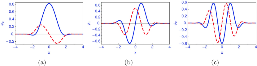
Figure 1: (Color online.) Figure (a) displays the ground-state wave function of the imaginary cubic Hamiltonian (43) for $G=1.0$. This wave function is manifestly complex. The real part $\mathrm{Re}\,\psi_{0}(x)$ (even under parity) is plotted using solid lines, and the dashed curve corresponds to the parity-odd imaginary part $\mathrm{Im}\,\psi_{0}(x)$. For the first excited state (still, $G=1.0$), the real part is odd, while the imaginary part is even under parity [see Fig. (b)]. The second excited state [Fig. (c)] has an even real part, while its imaginary part is odd. The global complex phase of the wave function is chosen so that the real part $\mathrm{Re}\,\psi_{n=0,1,2}(x)$ of the wave functions has the same qualitative behavior as the eigenstate wave function of the quartic oscillator displayed in Fig. 2(a).

II.4 Numerical reference data

The algorithmic procedure described above leads to a matrix diagonalization algorithm for complex symmetric matrices, which can find both the eigenvalues and eigenvectors of the original input matrix ${\bm{A}}$. We have checked numerical results obtained for wide classes of $\mathcal{PT}$-symmetric anharmonic oscillators against numerous published data. An example of an interesting alternative procedure for the calculation of the eigenenergies is given by the moment method HaBe1985 ; HaBeMo1988 ; HaBeSiMo1988 , which relies on a Fourier transformation of the Schrödinger equation and is based on a recursive calculation of the moments which define the series expansion of the wave function in momentum space. Applied to the positive-definite measure $S(x)=|\psi(x)|^{2}$, the method has been shown to generate numerical approximations for the discrete states of the $-{\rm i}\,x^{3}$ non-Hermitian potential Ha2001letter , as well as a potential proportional to $\mathrm{i}\,x^{3}+\mathrm{i}\,\alpha\,x$, which induces $\mathcal{PT}$ -symmetry breaking, manifestly complex eigenvalues HaKhWaTy2001 ; Ha2001long . The wave functions of eigenstates have also been studied, including Stokes and Anti-Stokes lines, for both the imaginary cubic oscillator HaWa2001 as well as generalized $(\mathrm{i}\,x)^{N}$-potentials YaHa2001 . Furthermore, we have used the algorithm for the calculation of resonance and anti-resonance energies of the “real” cubic perturbation (potential proportional to $x^{3}$) and other odd anharmonic oscillators. We note that the eigenvalues of the $\mathcal{PT}$-symmetric imaginary cubic perturbation and the Hermitian, but not essentially self-adjoint real cubic oscillator are related by a dispersion relation JeSuZJ2009prl ; BeDu1999 .

For reference, let us consider the two Hamiltonians

$$h_{3}= \;-\frac{1}{2}\,\mathrm{e}^{-2\mathrm{i}\theta}\,\partial_{x}^{2}+\frac{1}{2}\,\mathrm{e}^{2\mathrm{i}\theta}\,x^{2}+\mathrm{e}^{3\mathrm{i}\theta}\,x^{3}\,,\qquad 0<\theta<\frac{\pi}{5}\,,$$ (39a)

$$H_{3}= \;-\frac{1}{2}\,\partial_{x}^{2}+\frac{1}{2}\,x^{2}+\mathrm{i}\,x^{3}\,.$$ (39b)

The first of these involves a complex scaling transformation, which gives rise to manifestly complex resonance energy eigenvalues. The complex scaling transformation is “dual” to the resummation of the perturbation series to the complex resonance energies, which has been discussed in Refs. FrGrSi1985 ; Je2001pra ; Ca2003 . Using a multi-precision arithmetic implementation Ba1994tech ; Ba1995 of the algorithm described in Sec. II, we easily obtain the first two resonance energy eigenvalue of $h_{3}$ as follows,

$$\epsilon_{0}=0. 61288\,84333\,07754\,62425\,88175\,01988\,65141\,37333\,39788\,30718\,29420\,66181$$

$$-0. 40859\,26669\,32267\,28315\,94988\,68767\,16051\,62709\,74834\,43840\,39990\,97532\,\mathrm{i}\,,$$ (40a)

$$\epsilon_{1}=2. 18041\,38375\,36348\,77123\,01619\,63541\,74113\,12471\,72136\,83505\,89744\,59041$$

$$-1. 52620\,76556\,93032\,51000\,68539\,46967\,49562\,44459\,06099\,84880\,44103\,55220\,\mathrm{i}\,.$$ (40b)

All of the given decimals are significant; the 60-figure precision is obtained in a basis of roughly 1000 harmonic oscillator eigenstates and can be enhanced if desired. The ground-state-energy of the Hamiltonian $H_{3}$ and its first-excited-state energy reads as follows,

$$E_{0}=0. 79734\,26075\,08906\,18903\,90809\,60791\,01316\,30972\,44534\,48033\,11575\,78578\,,$$ (41a)

$$E_{1}=2. 77352\,49851\,95379\,71540\,58170\,00015\,53014\,23108\,48902\,82968\,52057\,22959\,.$$ (41b)

We again reemphasize that the precision of these results can be easily enhanced, as it was necessary to test some of the conjectured generalized quantization conditions for anharmonic oscillators presented in Refs. JeSuLuZJ2008 ; JeSuZJ2009prl ; JeSuZJ2010 ; ZJJe2010jpa . For typical double-precision (16 decimals) and quadruple-precision (32 decimals) calculations, we observe that the timings for matrix diagonalization using our algorithm are comparable to those using the routine ZGEEVX built into the LAPACK library AnEtAl1999 . Using a dedicated, concise implementation of the algorithm of the algorithm discussed in Sec. II.2 and Sec. II.3, we were even able to obtain timings which exceed the speed of LAPACK’s by up to 50% for typical applications (matrices of rank $500\times 500$); however, the speed-up may be compiler-specific (we were using gfortran version 4.7.2, see Ref. gfortran ).

III Pseudo–Hermitian Quantum Mechanics

III.1 Orientation

Let us try to explore the physical motivation for the construction of the matrix diagonalization algorithm presented in Sec. II, on the basis of pseudo-Hermitian ($\mathcal{PT}$-symmetric) quantum mechanics. A $\mathcal{PT}$-symmetric Hamilton operator $H$ fulfills the relation

$$H=\mathcal{P}\;\mathcal{T}\;H\;\mathcal{T}\;\mathcal{P}=\mathcal{P}\;H^{\mbox{{\bf{\tiny+}}}}\;\mathcal{P}\,,$$ (42)

where $H^{\mbox{{\bf{\tiny+}}}}$ is obtained BeBrReRe2004 from $H$ by the replacement $\mathrm{i}\to-\mathrm{i}$, which is the same as the Hermitian adjoint if all other terms in the Hamiltonian are explicitly real (rather than complex). The parity and time reversal are denoted as $\mathcal{P}$ and $\mathcal{T}$, respectively. If a Hamiltonian $H$ fulfills a relation of the type $H=\eta^{-1}\,H^{\mbox{{\bf{\tiny+}}}}\,\eta$, then $H$ is said to be pseudo-Hermitian Pa1943 . $\mathcal{PT}$-symmetry can thus be interpreted as a special case of pseudo-Hermiticity ($\eta=\mathcal{P}$), even if there is a certain “clash” with the original definition from Ref. Pa1943 , where it was assumed that $\eta$ is a positive-definite operator. By contrast, $\mathcal{P}$ may have the negative eigenvalue $-1$.

For reference, we continue our analysis with the well-known imaginary cubic perturbation JeSuLuZJ2008 ; JeSuZJ2009prl ; JeSuZJ2010 ; ZJJe2010jpa ; BeBo1998 ; BeBoMe1999 , which we had already employed in Sec. II.4. It is described by the Hamiltonian

$$H_{3}=-\frac{1}{2}\,\partial_{x}^{2}+\frac{1}{2}\,x^{2}+\mathrm{i}\,G\,x^{3}\,,\qquad G>0\,,$$ (43)

which for $G=1$ reduces to Eq. (39b). The eigenfunctions of $H_{3}$ are manifestly complex, in contrast to those of the quartic anharmonic oscillator,

$$H_{4}=-\frac{1}{2}\,\partial_{x}^{2}+\frac{1}{2}\,x^{2}+g\,x^{4}\,,\qquad g>0\,,$$ (44)

where the eigenstate wave functions can be chosen as purely real. For a $\mathcal{PT}$-symmetric system, the scalar product

$$\langle\psi(t)|\phi(t)\rangle_{\mathcal{P}\mathcal{T}}\equiv\int\mathrm{d}x\,\psi^{*}(x,t)\,\mathcal{P}\phi(x,t)$$ (45)

is conserved under time evolution if both $\psi$ and $\phi$ fulfill the time-dependent Schrödinger equation $\mathrm{i}\partial_{t}\psi(t)=H_{3}\psi(t)$, and $\mathrm{i}\partial_{t}\phi(t)=H_{3}\phi(t)$. However, the integrand in Eq. (45) is manifestly “nonlocal” because $\psi^{*}(x,t)\mathcal{P}\phi(x,t)=\psi^{*}(x,t)\phi(t,-x)$; it depends on function evaluations at $x$ and $-x$. This is in contrast to the ordinary scalar product

$$\langle\psi(t)|\phi(t)\rangle\equiv\int\mathrm{d}x\,\psi^{*}(x,t)\,\phi(x,t)\,,$$ (46)

where the first argument is complex conjugated, and the (generalized) indefinite inner product

$$\langle\psi(t)|\phi(t)\rangle_{*}\equiv\int\mathrm{d}x\,\psi(x,t)\,\phi(x,t)\,,$$ (47)

where none of the arguments are complex conjugated. The Hamiltonian $H_{3}$ given in Eq. (43) involves a manifestly complex potential, which we denote as $W(x)$,

$$W(x)= \;\frac{1}{2}\,x^{2}+\mathrm{i}\,G\,x^{3}=V(x)\,\mathrm{e}^{\mathrm{i}\,\arg(V(x))}\,,$$ (48a)

$$V(x)= \;|W(x)|=\sqrt{\tfrac{1}{4}\,x^{4}+G^{2}\,x^{6}}\,.$$ (48b)

The modulus $V(x)=|W(x)|$ tends to infinity as $x\to\pm\infty$. For purely real potentials like the “confining” quartic oscillator given in Eq. (44), intuition suggests that the “bulk” of the probability density of the eigenstate wave function should be concentrated in the “classically allowed” region, i.e., in the region where the eigenenergy $E$ is greater than the potential, i.e., $E>V(x)$ [where $V(x)\in\mathbbm{R}$]. For a manifestly complex potential, the condition $E>W(x)$ [with $W(x)\in\mathbbm{C}$] cannot be applied because the complex numbers are not ordered. In the following, we consider a few example calculations of energy eigenvalues of the imaginary cubic perturbation (43), which illustrate these observations. All of these have been accomplished using the algorithm presented in Sec. II.

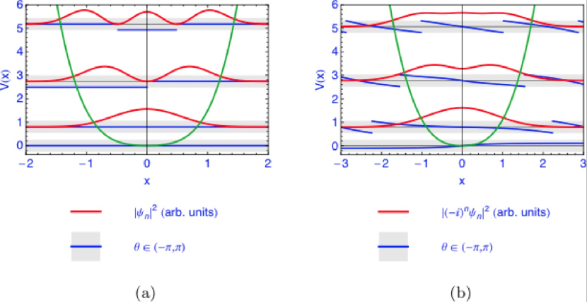
Figure 2: (Color online.) In Fig. (a), we plot the probability density $\rho=|\psi(x)|^{2}$ of the quartic oscillator’s ground state and first two excited states, in a potential $V(x)=\tfrac{1}{2}x^{2}+g\,x^{4}$ with $g=1.0$. Although the wave functions of the quartic potential are purely real, we use a modulus-phase plot for the real wave functions in Fig. (a). A sign change then corresponds to a jump in the complex phase from zero (for a positive real number) to $-\pi$ (for a positive negative number). In Fig. (b), we give a modulus-phase plot of the eigenstate wave functions of the imaginary cubic perturbation, where the complex phase of the wave function is displayed in the shaded region. The complex phase $\theta=\theta(x)$ in the decomposition $(-\mathrm{i})^{n}\,\psi_{n}(x)=|\psi_{n}(x)|\,\exp[\mathrm{i}\,\theta(x)]$ covers the interval $[-\pi,\pi)$. Here, the $\psi_{n}$ are the wave functions of Fig. 1, multiplied by a phase factor $(-\mathrm{i})^{n}$ [see also Eq. (52)].

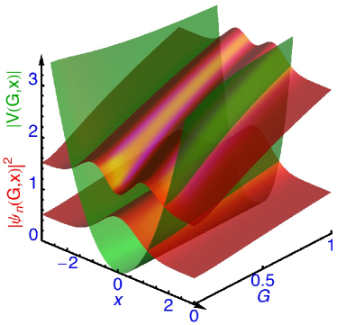
Figure 3: (Color online.) Illustration of the confinement mechanism for the imaginary cubic potential described by the Hamiltonian (43), for the ground and the first excited state. The bulk of the modulus square of the wave function is centered in the “allowed” region where the (real rather than complex) energy $E>V(x)=V(G,x)=|W(G,x)|$. The potential is plotted in green (the “trough”-like structure), whereas the moduli of the wave functions are plotted in red (the “wave-like structures”). The squares of the moduli of the wave functions either have a single maximum (ground state), or two maxima (first excited state). The ground state wave function has a modulus square $|\psi_{0}(x)|^{2}=|\psi_{0}(G,x)|^{2}$ as a function of $G$ and $x$. As $G$ increases, the bound-state energy (which is equal to the base line of the wave function curve at any given value of $G$) increases, and the modulus of the potential forms a more narrow trough to which the ground-state wave function is confined. The same is true for the first excited state. The central minimum of the modulus square of the first-excited state wave function is clearly visible.

III.2 Example calculations

We can formally split the Hamiltonian $H_{3}$ into a “real part” and a “imaginary part” as follows,

$$\mathrm{Re}\,H_{3}= \;-\tfrac{1}{2}\,\partial_{x}^{2}+\tfrac{1}{2}x^{2}\,,\qquad\mathrm{Im}\,H_{3}=\mathrm{i}\,G\,x^{3}\,.$$ (49)

Likewise, we can also split the eigenstate wave function $\psi_{n}(x)$ into real and imaginary parts,

$$\psi_{n}(x)=\mathrm{Re}\,\psi_{n}(x)+\mathrm{i}\,\mathrm{Im}\,\psi_{n}(x)\,.$$ (50)

Based on the decomposition (49), one can show that if $\mathrm{Re}\,\psi_{n}(x)$ is even under parity and $\psi_{n}(x)$ is an eigenstate of $H_{3}$ with real eigenvalue of $\epsilon_{n}$, then $\mathrm{Im}\,\psi_{n}(x)$ has to be parity-odd, and vice versa. Also, if $\mathrm{Re}\,\psi_{n}(x)$ is odd under parity, then $\mathrm{Im}\,\psi_{n}(x)$ has to be even under parity. Because the parity operator $\mathcal{P}$ does not commute with the Hamiltonian $H_{3}$, the eigenstates of $H_{3}$ are not eigenstates of parity. Furthermore, because the potential is manifestly complex, so are the wave functions. Yet, numerical evidence drawn from Fig. 1 suggests that if the global phase of the wave function is appropriately chosen, both real as well as imaginary parts of the eigenstates are eigenstates of parity, individually. These eigenstates are naturally obtained if one diagonalizes an approximation to the cubic Hamiltonian obtained by projection onto a suitably large basis set of harmonic oscillator eigenstates.

The antilinear $\mathcal{P}\mathcal{T}$ operator commutes with the Hamiltonian, and the eigenfunctions of $H_{3}$ are also $\mathcal{P}\mathcal{T}$ eigenstates BeBrReRe2004 . The precise eigenvalue of $\mathcal{PT}$ may, however, depend on the phase assigned to $\psi_{n}(x)$ because $\mathcal{T}$ is an antilinear operator. Let us first investigate the phase conventions used in Fig. 1, where the real and imaginary parts of the wave function are, alternatingly, even and odd under parity as we proceed to higher excited states. The appropriate eigenvalues are thus

$$\mathcal{P}\mathcal{T}\psi_{n}(x)=\psi^{*}_{n}(-x)=(-1)^{n}\,\psi(x)\,.$$ (51)

However, the eigenvalue of the wave functions $\Psi_{n}(x)=(-\mathrm{i})^{n}\psi_{n}(x)$ with respect to the $\mathcal{P}\mathcal{T}$ operator is unity,

$$\mathcal{P}\mathcal{T}[(-\mathrm{i})^{n}\,\psi_{n}(x)]=\mathrm{i}^{n}\,\psi^{*}_{n}(x)=[(-\mathrm{i})^{n}\,\psi(x)]\,.$$ (52)

For two eigenstates of the $\mathcal{PT}$-symmetric system, the conserved $\mathcal{PT}$-symmetric scalar product simply is the indefinite inner product, as defined in Eq. (2.4.2) of Ref. Mo1998 ,

$$\langle\Psi_{n}|\Psi_{m}\rangle_{\mathcal{P}\mathcal{T}}= \;\int\mathrm{d}x\,\Psi_{n}^{*}(x)\mathcal{P}\Psi_{m}(x)=\int\mathrm{d}x\,\left(\mathcal{P}\mathcal{T}\Psi_{n}\right)(x)\,\Psi_{m}(x)$$

$$= \;\int\mathrm{d}x\,\Psi_{n}(x)\,\Psi_{m}(x)=\langle\Psi_{n}|\Psi_{m}\rangle_{*}\,.$$ (53)

The integrand in Eq. (III.2) is “local” in the sense that it depends only on wave functions at $x$, not $-x$. The non-local character of the integrand in Eq. (45) has otherwise been called into question and has given rise to rather sophisticated attempts at finding an alternative, appropriate interpretation AbJaPa2013 . The natural normalization condition for eigenstates of complex, symmetric matrices (including infinite-dimensional matrices) is given by Mo1998

$$\langle\psi_{n}|\psi_{m}\rangle_{*}=\delta_{nm}\,,\qquad\langle\Psi_{n}|\Psi_{m}\rangle_{*}=(-1)^{n}\,\delta_{nm}\,,$$ (54)

and involves the indefinite inner product defined in Eq. (47). The equivalence shown in Eq. (III.2) and the orthogonality properties (54) provide the main motivation for the construction of the generalized Householder transformation (2); indeed, the generalized inner product (III.2) reduces to (1) for finite-dimensional vector spaces. “Half” of the $\Psi_{n}$ eigenstates acquire a negative $\mathcal{PT}$-symmetric norm, as described by the prefactor $(-1)^{n}$. For two time-dependent states of the $\mathcal{PT}$-symmetric system, given as

$$\chi(t)=\sum_{n}a_{n}(t)\;|\Psi_{n}\rangle\,,\quad\rho(t)=\sum_{m}b_{m}(t)\;|\Psi_{m}\rangle\,,$$ (55)

with $a_{n}=(-1)^{n}\,\langle\Psi_{n}|\chi\rangle$, and $b_{n}=(-1)^{n}\,\langle\Psi_{n}|\rho\rangle$, the $\mathcal{PT}$-symmetric scalar product is calculated as follows,

$$\langle\chi(t)|\rho(t)\rangle_{\mathcal{P}\mathcal{T}}= \;\sum_{nm}a^{*}_{n}(t)\,b_{m}(t)\,\int\mathrm{d}x\,\Psi_{n}^{*}(x)\mathcal{P}\Psi_{m}(x)=\sum_{nm}a^{*}_{n}(t)\,b_{m}(t)\,\int\mathrm{d}x\,\Psi_{n}(x)\Psi_{m}(x)$$

$$= \;\sum_{n}(-1)^{n}\,a^{*}_{n}(t)\,b_{n}(t)=\langle\vec{a}(t)|\vec{b}(t)\rangle_{\rm even}-\langle\vec{a}(t)|\vec{b}(t)\rangle_{\rm odd}\,.$$ (56)

with an obvious identification of $\langle\vec{a}(t)|\vec{b}(t)\rangle_{\rm even}$ and $\langle\vec{a}(t)|\vec{b}(t)\rangle_{\rm odd}$. Note that one cannot suppress the factor $(-1)^{n}$ in the second-to-last line of Eq. (III.2) by a change in the global phase factor of the wave functions. The factor either occurs because of the $\mathcal{PT}$-symmetric eigenvalue of the $\psi_{n}$, or because of the alternating sign of the norm of the $\Psi_{n}$. The $\mathcal{PT}$-symmetric time evolution is separately unitary in the space of the coefficients $a_{n}(t)$, $b_{n}(t)$ with (i) even $n$ and (ii) odd $n$, as denoted by an appropriate subscript in Eq. (III.2). In some sense, the $\mathcal{PT}$-symmetric time evolution leads to a natural “splitting” of the Hilbert space into two subspaces, those of the function with negative $\mathcal{PT}$-symmetric norm and those with positive norm, according to the second equality in Eq. (54). The same pattern has recently been observed in a field-theoretical context JeWu2012epjc ; JeWu2013isrn : Half of the states of the generalized Dirac equation with a pseudo-scalar mass term acquire a negative Fock-space norm.

From ordinary, Hermitian, quantum mechanics, it is known that the $L^{2}(\mathbbm{R})$ eigenfunctions of a Hermitian operator are in some sense confined to spatial regions where the eigenenergy $E_{n}$ is larger than the local value of the potential, $E>V(x)$. An intuitive understanding can be obtained if we interpret the potential in terms of a modulus and a phase, according to Eq. (48a). We use the rationale of accompanying a plot of the modulus of a function by a grey band to convey complex phase information in Figs. 2 and 3, where the complex eigenstate wave functions shown previously in Fig. 1 are plotted in terms of the decomposition

$$\psi_{n}(x)=|\psi_{n}(x)|\,\mathrm{e}^{\mathrm{i}\,\arg(\psi_{n}(x))}\,.$$ (57)

The curves in Figs. 2 and 3 show that indeed, the wave functions of the $\mathcal{PT}$-symmetric oscillator are concentrated [in the sense of a large absolute value of the integrand in Eq. (III.2)] to a region where $E_{n}>V(x)=|W(x)|$, where $W(x)$ is the complex-valued $\mathcal{PT}$-symmetric potential (48a). In Fig. 3, we illustrate that the “confinement” mechanism holds for all values in the range $0<G<1$. The interlacing of zeros in complex Sturm–Liouville problems for $\mathcal{PT}$-eigenfunctions, has been discussed in Ref. BeBoSa2000 . In agreement with the conclusions of Ref. BeBoSa2000 , we find that both the real as well as imaginary parts of the complex eigenfunctions have an infinite number of zeros, individually, when the argument $x$ of the wave function covers the real numbers. Furthermore, this statement even holds for an infinitesimally small, but nonvanishing coupling $G$ in the imaginary cubic perturbation $\mathrm{i}\,G\,x^{3}$.

IV Conclusions

In Sec. II, we have presented an efficient algorithm for the calculation of eigenvalues of complex symmetric (not Hermitian) matrices. The algorithm is scalable in terms of the desired numerical accuracy and relies on generalized Householder reflections which “depopulate” the input matrix by projecting the entries onto the sub- and super-diagonals, using the generalized inner product which avoids the complex conjugation of the first argument. We find that a subsequent diagonalization of the tridiagonal matrix obtained from the Householder transformations, using generalized Jacobi and Givens rotation matrices (which are again complex and symmetric but not unitary) leads to an efficient eigenvalue solver. Numerical reference data are provided in Sec. II.4, and we reemphasize that many of the previously reported numerical tests of generalized quantization conditions for anharmonic oscillators JeSuLuZJ2008 ; JeSuZJ2009prl ; JeSuZJ2010 ; ZJJe2010jpa rely on the numerical methods described in this paper. The indefinite inner product can indeed be useful in numerical algorithms; in Ref. ArHo2004 , the indefinite inner product had been used previously in a reformulation of the Rayleigh quotient, within an adaptation of the Jacobi–Davidson method for complex symmetric matrices (which has nothing to do with the Jacobi rotations used in our algorithm). We might add that in contrast to the Jacobi–Davidson method, our algorithm does not require a Gram–Schmidt orthogonalization step and is based on a generalized inner product which draws its inspiration from physics.

We would like to illustrate and comment on the algorithm by pointing out a few possible modifications and intricacies of the methods used. The above version of the algorithm described in Sec. II is based on the QL rather than QR decomposition. In the (shifted) iterated QL decomposition, one starts the calculation of the eigenvalue guess from the upper left corner of the input matrix but calculates the Givens and Jacobi rotations from the lower right, i.e., one “chases the bulge upward”. In that case, the “uppermost” eigenvalue of the input matrix converges first; the guess $\sigma$ approximates the true eigenvalue to machine accuracy. If the complex symmetric Hamiltonian is obtained from a basis set of “trial” quantum states the first of which approximates the state of lowest energy of the perturbed system, then the QL decomposition as opposed to the QR decomposition ensures that the “ground-state energy converges first”. Still, it is an instructive exercise to modify the algorithm so that the “eigenvalue guess” $\sigma$ is first calculated for the “lower rightmost” eigenvalue. One then calculates the Jacobi and Givens rotations which “chase the bulge” from the upper left to the lower right of the tridiagonal matrix. In that case, the “lower rightmost” eigenvalue converges first. This may be useful in particular cases where the “highest” eigenvalue is of particular interest.

One has a few options for controlling the convergence of the algorithm: For example, in many applications, the element $D_{i}$ may be declared to have “converged” if $D_{i}+E_{i}$ equals $D_{i}$ to machine accuracy, but this criterion may be too restrictive in some cases, especially, when multi-precision arithmetic is being used. In that case, it should be replaced by a criterion which states that $|D_{i}/E_{i}|$ is less than a specific, predefined accuracy, say $10^{-64}$ (for so-called “octuple precision” arithmetic, with 64 decimals).

Our QL factorization involves manifestly complex symmetric ${\bm{Q}}$ matrices. Typically, routines built into modern computer algebra system use a unitary matrix ${\bm{Q}}$ for such decompositions. These routines use manifestly different matrices than those employed in the approach described above and therefore cannot be used, say, in a meaningful comparison to an implementation of the above algorithm.

In the iterated, shifted QL decomposition of the tridiagonal matrix ${\bm{T}}$, the most common pitfall consists in a “premature zero”, i.e., in an entry on the sub- or super-diagonal $E_{j}$ which becomes zero to machine accuracy before the “target element” $E_{i<j}$ for which the current guess $\sigma$ is calculated has converged to the desired accuracy. In that case, the tridiagonal matrix naturally divides into two matrices (two “irreducible representations”) which have to be considered separately. Typically, this phenomenon occurs when the entries in the original input matrix ${\bm{A}}$ have a somewhat irregular pattern (e.g., random matrices). The necessity to partition the tridiagonal matrix upon the occurrence of premature zeroes is described rather scarcely in the literature; some lecture notes on the matter can be found in Sec. 11.4 of  Fa2006 and near the end of Sec. 3.6.2 of Ref. Ar2012 . The division into two matrices is called “partitioning” in Sec. 4.7 of  He1991 . For matrices obtained from regularly distributed, trial basis states, which typically occur in theoretical physics, we have not observed this phenomenon.

As a final remark, we would like to mention that a plain iterated QL or QR decomposition leads to a rather efficient, but not optimized, convergence of the eigenvalues problem, especially for regular input entries in the matrix ${\bm{A}}$. The QL and QR decompositions of the input matrix ${\bm{A}}$ can be calculated using generalized Householder reflections: For QL, one starts from the rightmost column vector of ${\bm{A}}$ and projects it onto its last element; for QR, on starts from the leftmost column vector of ${\bm{A}}$ and projects it onto its first element; the subsequent Householder reflections are constructed from the “deflated” $(n-1)\times(n-1)$ submatrices, in either direction GovL1996 ; Pa1998matrix . Skipping the tridiagonalization step, one can thus construct generalized QL and QR factorization-based matrix diagonalization routines where ${\bm{Q}}$ is manifestly complex and symmetric, but not unitary. Otherwise, the implicit shift (29) leads to improved convergence toward to numerical approximations of the eigenvalues.

The usefulness of the generalized Householder reflections used in the algorithm has a connection to the underlying physics. Indeed, we find that the most natural interpretation of the conserved scalar product in the $\mathcal{PT}$-symmetric time evolution is in terms of the generalized indefinite inner product defined for finite-dimensional vectors in Eq. (1) and for Hilbert space vectors in Eq. (47). This inner product is linear in both arguments and avoids complex conjugation. Attempts at finding an alternative, appropriate interpretation AbJaPa2013 seem too complicated to take precedence over the immediate identification of the $\mathcal{PT}$-symmetric scalar product of eigenvectors in terms of the indefinite inner product. The integrand immediately becomes “local” and one avoids integrations over eigenfunctions evaluated at the (possibly very distant) points $x$ and $-x$. We reemphasize that the indefinite inner product is crucial in the analysis of resonance eigenvectors Mo1998 for the “real” cubic perturbation, and that the eigenvalues of the “real” and “imaginary” cubic perturbation are related by a dispersion relation BeDu1999 ; JeSuZJ2009prl . So, in some sense, the importance of the indefinite inner product for the analysis of the imaginary cubic Hamiltonian had to be expected, and the emergence of an efficient matrix diagonalization algorithm for such matrices is only natural (see Sec. III).

It has been stressed in the literature that the scalar product $\langle\psi(t)|\phi(t)\rangle_{\mathcal{P}\mathcal{T}}$ as defined in Eq. (45) is not positive definite. This has been used as an argument against the viability of $\mathcal{PT}$-symmetric Hamiltonians for the description of natural phenomena. However, one may counter argue that the same problem persists with regard to the relativistic Klein-Gordon equation where the time-like component of the conserved Noether current can become negative (see Chap. 2 of Ref. ItZu1980 ). The Klein-Gordon equation is assumed to describe a charged scalar field like the charged component of the Higgs (doublet) field PeSc1995 (the latter is usually assumed to vanish under a gauge transformation, and the remaining neutral component of the Higgs doublet is expanded about its vacuum expectation value). Strictly speaking, one has to reinterpret the timelike component of the conserved Noether current as a charge density, not a probability density. Analogously, the timelike component of the conserved Noether current of the pseudo–Hermitian, generalized Dirac Hamiltonian (with a pseudo-scalar mass term) may naturally be interpreted as a non-positive definite “weak-interaction density” (see Ref. JeWu2013isrn ). Equation (III.2) suggests that the Hilbert space, under the $\mathcal{PT}$-symmetric time evolution, is split into two “halves”, one of which entails negative $\mathcal{PT}$-symmetric norm (analogous to the “right-handed neutrinos”), and the other has positive $\mathcal{PT}$-symmetric norm (analogous to the “left-handed neutrinos” within the model proposed in Ref. JeWu2013isrn ). We recall that “half” of the $\Psi_{n}$ eigenstates acquire a negative $\mathcal{PT}$-symmetric norm under a very natural choice of the global complex phase [see Eq. (55)]. The $\mathcal{PT}$-symmetric norm, in turn, can be formulated in terms of the generalized indefinite inner product, on which this article is based.

References

- (1) U. D. Jentschura, A. Surzhykov, M. Lubasch, and J. Zinn-Justin, J. Phys. A 41, 095302 (2008).
- (2) U. D. Jentschura, A. Surzhykov, and J. Zinn-Justin, Phys. Rev. Lett. 102, 011601 (2009).
- (3) U. D. Jentschura, A. Surzhykov, and J. Zinn-Justin, Ann. Phys. (N.Y.) 325, 1135 (2010).
- (4) J. Zinn-Justin and U. D. Jentschura, J. Phys. A 43, 425301 (2010).
- (5) C. M. Bender and S. Boettcher, Phys. Rev. Lett. 80, 5243 (1998).
- (6) C. M. Bender, S. Boettcher, and P. N. Meisinger, J. Math. Phys. 40, 2201 (1999).
- (7) C. M. Bender and G. V. Dunne, J. Math. Phys. 40, 4616 (1999).
- (8) C. M. Bender and T. T. Wu, Phys. Rev. 184, 1231 (1969).
- (9) C. M. Bender and T. T. Wu, Phys. Rev. Lett. 27, 461 (1971).
- (10) J. Stoer and R. Bulirsch, Introduction to Numerical Analysis, 3 ed. (Springer, Berlin, 2002).
- (11) J. H. Wilkinson, The Algebraic Eigenvalue Problem (Oxford University Press, Oxford, UK, 1965).
- (12) J. H. Wilkinson and C. H. Reinsch, Linear Algbera. Handbook for Automatic Computation (Springer, Heidelberg, 1971).
- (13) G. Golub and C. F. van Loan, Matrix Computations, 3 ed. (The Johns Hopkins University Press, Baltimore, MD, 1996).
- (14) B. N. Parlett, The Symmetric Eigenvalue Problem (Prentice Hall, Englewood Cliffs, NJ, 1998).
- (15) E. Anderson, Z. Bai, C. Bischof, S. Blackford, J. Demmel, J. Dongarra, J. Du Croz, A. Greenbaum, S. Hammarling, A. McKenney, and D. Sorensen, LAPACK Users’ Guide, 3 ed. (Society for Industrial and Applied Mathematics, Philadelphia, PA, 1999).
- (16) C. M. Bender, J. Brod, A. Refig, and M. E. Reuter, J. Phys. A 37, 10139 (2004).
- (17) I. C. Gohberg, P. Lancaster, and L. Rodman, Matrices and Indefinite Scalar Products, Oper. Theory Adv. Appl. 8, Birkhäuser Verlag, Basel, 1983.
- (18) N. Moiseyev, Phys. Rep. 302, 211 (1998).
- (19) P. Arbenz and M. E. Hochstenbach, SIAM J. Sci. Comput. 25, 1655 (2004).
- (20) J. G. F. Francis, The Computer Journal 4, 265 (1961).
- (21) J. G. F. Francis, The Computer Journal 4, 332 (1962).
- (22) J. H. Wilkinson, Lin. Alg. Applic. 1, 409 (1968).
- (23) S. Wolfram, The Mathematica Book, 4 ed. (Cambridge University Press, Cambridge, UK, 1999).
- (24) C. G. J. Jacobi, Crelle’s Journal 30, 51 (1846).
- (25) W. Givens, J. Soc. Indust. Appl. Math. 6, 26 (1958).
- (26) C. R. Handy and D. Bessis, Phys. Rev. Lett. 55, 931 (1985).
- (27) C. R. Handy, D. Bessis, and T. D. Morley, Phys. Rev. A 37, 4557 (1988).
- (28) C. R. Handy, D. Bessis, G. Sigismondi, and T. D. Morley, Phys. Rev. Lett. 60, 253 (1988).
- (29) C. R. Handy, J. Phys. A 34, L271 (2001).
- (30) C. R. Handy, D. Khan, X.-Q. Wang, and C. J. Tymczak, J. Phys. A 34, 5593 (2001).
- (31) C. R. Handy, J. Phys. A 34, 5065 (2001).
- (32) C. R. Handy and X. Q. Wang, J. Phys. A 34, 8297 (2001).
- (33) Z. Yan and C. R. Handy, J. Phys. A 34, 9907 (2001).
- (34) V. Franceschini, V. Grecchi, and H. J. Silverstone, Phys. Rev. A 32, 1338 (1985).
- (35) U. D. Jentschura, Phys. Rev. A 64, 013403 (2001).
- (36) E. Caliceti, J. Math. Phys. 44, 2026 (2003).
- (37) D. H. Bailey, A Fortran-90 based multiprecision system, NASA Ames Tech. Rep. RNR-94-013, published as ACM Trans. on Mathematical Software 21, 379 (1995).
- (38) D. H. Bailey, ACM Trans. Math. Soft. 21, 379 (1995).
- (39) The gfortran compiler is available at the URL http://hpc.sourceforge.net.
- (40) W. Pauli, Rev. Mod. Phys. 15, 175 (1943).
- (41) K. Abhinav, A. Jayannavar, and P. K. Panigrahi, Ann. Phys. (N.Y.) 331, 110 (2013).
- (42) U. D. Jentschura and B. J. Wundt, Eur. Phys. J. C 72, 1894 (2012).
- (43) U. D. Jentschura and B. J. Wundt, ISRN High Energy Physics 2013, 374612 (2013).
- (44) C. M. Bender, S. Boettcher, and V. M. Savage, J. Math. Phys. 41, 6381 (2000).
- (45) G. Fasshauer, The QR Algorithm, in lecture notes on 477/577 Numerical Linear Algebra/Computational Mathematics I, available at the URL http://www.math.iit.edu/ fass/477577_Chapter_11.pdf.
- (46) P. Arbenz, The QR Algorithm, Chapter 3 of the lecture notes on Numerical Methods for Solving Large Scale Eigenvalue Problems, available at the URL http://people.inf.ethz.ch/arbenz/ewp/Lnotes/chapter3.pdf.
- (47) L. E. Henderson, Testing eigenvalue software, PhD Thesis, University of Arizona, USA (1991), unpublished, available at the URL http://arizona.openrepository.com/arizona/bitstream/10150/185744/1/azu_td_9213693_sip1_m.pdf.
- (48) C. Itzykson and J. B. Zuber, Quantum Field Theory (McGraw-Hill, New York, 1980).
- (49) M. E. Peskin and D. V. Schroeder, An Introduction to Quantum Field Theory (Perseus, Cambridge, Massachusetts, 1995).