NUCLEAR ASYMMETRY ENERGY AND ISOVECTOR STIFFNESS WITHIN THE EFFECTIVE SURFACE APPROXIMATION

Abstract

The isoscalar and isovector particle densities in the effective surface approximation to the average binding energy are used to derive analytical expressions of the surface symmetry energy, the neutron skin thickness and the isovector stiffness of sharp edged proton-neutron asymmetric nuclei. For most Skyrme forces the isovector coefficients of the surface energy and of the stiffness are significantly different from the empirical values derived in the liquid drop model. Using the analytical isovector surface energy constants in the framework of the hydrodynamical and the Fermi-liquid droplet models the mean energies and the sum rules of the isovector giant dipole resonances are found to be in fair agreement with the experimental data.

Keywords: Nuclear binding energy, liquid droplet model, extended Thomas-Fermi approach, nuclear surface energy, symmetry energy, neutron skin thickness, isovector stiffness.

PACS numbers: 21.10.Dr, 21.65.Cd, 21.60.Ev, 21.65.Ef

I Introduction

A simple and accurate solution of particle-density distributions was obtained within the nuclear effective surface (ES) approximation in Refs. strtyap ; strmagbr ; strmagden . It exploits the saturation properties of nuclear matter in the narrow diffuse-edge region in finite heavy nuclei. The ES is defined as the location of points with a maximum density gradient. An orthogonal coordinate system related locally to the ES is specified by the distance $\xi$ of a given point from this surface and tangent coordinates $\eta$ parallel to the ES (see Fig. 1). Using nuclear energy density functional theory, the variational condition derived from minimizing the nuclear energy at some fixed integrals of motion is simplified in the $\xi,\eta$ coordinates. In particular, in the extended Thomas-Fermi (ETF) approach brguehak , it can be done for any fixed deformation using the expansion in a small parameter $a/R\sim A^{-1/3}\ll 1$ for heavy enough nuclei, where $a$ is of the order of the diffuse-edge thickness of the nucleus, $R$ is the mean curvature radius of the ES, and $A$ is the number of nucleons. The accuracy of the ES approximation in the ETF approach without spin-orbit (SO) and asymmetry terms was checked strmagden by comparing results with those of the Hartree-Fock (HF) and ETF theories for some Skyrme forces. The ES approach strmagden was also extended by taking into account the SO and asymmetry effects magsangzh .

In the present work, solutions for the isoscalar and isovector particle densities and energies in the ES approximation of the ETF approach are applied to analytical calculations of the surface symmetry energy, the neutron skin, and the isovector stiffness coefficient in the leading order of the parameter $a/R$ (see also Ref. BMV ). Our results are compared with older investigations myswann69 ; myswnp80pr96 ; myswprc77 ; myswiat85 in the liquid droplet model (LDM) and with more recent works danielewicz1 ; pearson ; danielewicz2 ; vinas1 ; vinas2 ; vinas3 ; vinas4 ; kievPygmy ; nester . We suggest also studying also the splitting of the isovector giant dipole resonances into main and satellite (pygmy) peaks kievPygmy ; nester as a function of the analytical isovector surface energy constant of the ES approach within the Fermi-liquid droplet (FLD) model denisov ; kolmag ; kolmagsh . The analytical expressions for the surface symmetry energy constants are tested by the mean energies of the isovector giant dipole resonances (IVGDR) within the hydrodynamical (HD) and FLD models.

The manuscript is organized as follows: In Sec. II we give an outlook of the basic points of the ES approximation within the density functional theory, and the main results for the isoscalar and isovector particle densities. Section III is devoted to analytical derivations of the symmetry energy in terms of the surface energy coefficient, the neutron skin thickness, and the isovector stiffness. The discussions of the results are given in Sec. IV and summarized in Sec. V. Some details of our calculations are presented in Appendixes A-C.

II Energy and particle densities

We start with the nuclear energy as a functional of the isoscalar and the isovector densities $\rho_{\pm}=\rho_{n}\pm\rho_{p}$:

$$E=\int\hbox{d}{\bf r}\;{\cal E}\left(\rho_{+},\rho_{-}\right)\;,$$ (1)

in the local density approach brguehak ; chaban ; reinhard ; bender ; revstonerein ; ehnazarrrein with the energy density ${\cal E}\left(\rho_{+},\rho_{-}\right)$,

$${\cal E}\left(\rho_{+},\rho_{-}\right) \approx -b_{V}\rho_{+}+JI^{2}\rho_{+}+\rho_{+}\left[\varepsilon_{+}(\rho_{+})-\varepsilon_{-}(\rho_{+},\rho_{-})\right]+$$ (2)

$$+ \left({\cal C}_{+}+{\cal D}_{+}\rho_{+}\right)\left(\nabla\rho_{+}\right)^{2}+\left({\cal C}_{-}+{\cal D}_{-}\rho_{+}\right)\left(\nabla\rho_{-}\right)^{2}\;,$$

where $~{}I=(N-Z)/A$ is the asymmetry parameter, $~{}N=\int\hbox{d}{\bf r}\rho_{n}({\bf r})$ and $~{}Z=\int\hbox{d}{\bf r}\rho_{p}({\bf r})$ are the neutron and proton numbers and $~{}A=N+Z$. As usual, the energy density ${\cal E}$ in Eq. (2) contains the volume part given by the first two terms of Eq. (2) and the surface part including the density gradients strtyap ; strmagden . The particle separation energy $b_{V}\approx$ 16 MeV and the symmetry energy constant of the nuclear matter $~{}J\approx$ 30 MeV specify the volume terms in Eq. (2). Equation (2) can be applied in a semiclassical approximation for realistic Skyrme forces chaban ; reinhard ; bender ; revstonerein ; ehnazarrrein , in particular by neglecting higher $\hbar$ corrections in the ETF kinetic energy brguehak ; strmagbr ; strmagden and Coulomb terms. Up to small Coulomb exchange terms they all can be easily taken into account (see Refs. strtyap ; strmagden ; magsangzh ). The constants ${\cal C}_{\pm}$ and ${\cal D}_{\pm}$ are defined by the parameters of the Skyrme forces chaban ; reinhard . The isoscalar part of the surface energy density, which does not depend explicitly on the density gradient terms, is determined by the function $\varepsilon_{+}(\rho_{+})$ strmagden ; magsangzh , which satisfies the saturation condition $\varepsilon_{+}(\overline{\rho})=0$, $(\hbox{d}\varepsilon_{+}(\rho_{+})/\hbox{d}\rho_{+})_{\rho_{+}=\overline{\rho}}=0$, where $\overline{\rho}=3/4\pi r_{0}^{3}\approx$ 0.16 fm^-3 is the density of the infinite nuclear matter and $r_{0}=R/A^{1/3}$ is the radius constant. Here we use a quadratic approximation, $\varepsilon_{+}=K(\rho_{+}-\overline{\rho})^{2}/(18\overline{\rho}^{2})$, where $K$ is the incompressibility modulus of symmetric nuclear matter, mainly $K\approx 220-260$ MeV (see Table I). The isovector component can be simply evaluated as $\varepsilon_{-}=J\;\left(I^{2}-\rho_{-}^{2}/\rho_{+}^{2}\right)$ magsangzh . The isoscalar SO gradient terms in Eq. (2) are defined with a constant: ${\cal D}_{+}=-9mW_{0}^{2}/16\hbar^{2}$, where $W_{0}\approx$100 - 130  MeV$\cdot$fm⁵ and $m$ is the nucleon mass brguehak ; chaban ; reinhard ; bender ; revstonerein .

Minimizing the energy $E$ under the constraints of the fixed particle number $A=\int\hbox{d}{\bf r}\;\rho_{+}({\bf r})$ and neutron excess $N-Z=\int\hbox{d}{\bf r}\;\rho_{-}({\bf r})$ (also others, such as deformation strtyap ; strmagden ), one arrives at the Lagrange equations with the corresponding multipliers, $\lambda_{+}$ and $\lambda_{-}$ being the isoscalar and isovector chemical potentials, respectively (see Appendixes A and B). Our approach can be applied for any deformation parameter of the nuclear surface if its diffuseness with respect to the curvature radius $a/R$ is small. The analytical solutions will be obtained approximately up to the order of $A^{2/3}$ in the binding energy. To satisfy the condition of particle number conservation with the required accuracy, we account for relatively small surface corrections ($\propto a/R\sim A^{-1/3}$ at the first order) to the leading terms in the Lagrange multipliers strmagbr ; strmagden ; magsangzh (Appendixes B and C).

For the isoscalar particle density, $w=\rho_{+}/\overline{\rho}$ one has up to leading terms in the parameter $a/R$ the usual first-order differential Lagrange equation with the solution strmagden ; magsangzh

$$x=-\int_{w_{r}}^{w}\hbox{d}y\;\sqrt{\frac{1+\beta y}{y\epsilon(y)}}\;,\qquad x=\frac{\xi}{a}\qquad\left(a=\sqrt{\frac{{\cal C}_{+}\;\overline{\rho}\;K}{30\;b_{V}^{2}}}\right)$$ (3)

below the turning point $x(w=0)$; $w=0$ for $x\geq x(w=0)$ and $\beta={\cal D}_{+}\overline{\rho}/{\cal C}_{+}$ is the dimensionless SO parameter. For convenience we introduced also the dimensionless parameter $\epsilon=18\varepsilon_{+}/K$. For $w_{r}=w(x=0)$ one has the boundary condition $\hbox{d}^{2}w(x)/\hbox{d}x^{2}=0$ at the ES ($x=0$):

$$\epsilon(w_{r})+w_{r}(1+\beta w_{r})\left[\hbox{d}\epsilon(w)/\hbox{d}w\right]_{w=w_{r}}=0\;\;.$$ (4)

In Eq. (3), $a\approx 0.5-0.6$ fm is the diffuseness parameter as shown in Table I ($\xi=r-R~{}$ for spherical nuclei in spherical coordinates). The diffuseness of the edge $a_{d}$ is given by

$$a_{d}=\sqrt{5(\overline{\xi^{2}}-\overline{\xi}^{2})/3}=a\sqrt{5(\overline{x^{2}}-\overline{x}^{2})/3}\;,\qquad\overline{x^{n}}=\int_{-\infty}^{\infty}x^{n}\hbox{d}x(\hbox{d}w/\hbox{d}x)\;,$$ (5)

where bars mean an averaging with the surface density distribution $dw/dx$ strmagden . For all Skyrme forces (Table I) the parameter $a$ introduced in Eq. (3) measures the diffuseness of the nuclear edge as the mean-squared fluctuation of $\xi$ due to the relation $a_{d}\approx a\sqrt{5/3}$ (see also Refs. strmagden ; vinas2 ). As shown in Ref. magsangzh , the influence of the semiclassical $\hbar$ corrections (related to the ETF kinetic energy) to $w(x)$ is negligibly small everywhere, besides the quantum tail outside the nucleus ($x\hbox{\kern 1.00006pt\lower 2.58334pt\hbox{$\sim$} \kern-11.19997pt\raise 2.58334pt\hbox{$>$} \kern 1.00006pt}1$). Therefore, all these corrections were neglected in Eq. (2). With a good convergence of the expansion of the $\epsilon(y)$ in powers of $1-y$ up to the quadratic term strmagden ; magsangzh , $\epsilon=(1-y)^{2}$, one finds the analytical solutions of Eq. (3) in terms of algebraic, trigonometric, and logarithmic functions [see Eq. (A3)]. For $\beta=0$ (i.e., without SO terms), it simplifies to the solution $w(x)=\tanh^{2}\left[(x-x_{0})/2\right]$ for $x\leq x_{0}=2{\rm arctanh}(1/\sqrt{3})$ and zero for $x$ outside the nucleus ($x>x_{0}$).

For the isovector density, $w_{-}(x)=\rho_{-}/(\overline{\rho}I)$, after simple transformations of the isovector Lagrange equation up to the leading term in $a/R$ in the ES approximation one similarly finds the equation and boundary condition [see Eq. (A2)]. The analytical solution for $w_{-}=w\hbox{cos}[\psi(w)/\sqrt{1+\beta}]$ can be obtained through the expansion (A5) of $\psi$ in powers of

$$\widetilde{w}(w)=(1-w)/c_{sym}\qquad\mbox{ with}\qquad c_{sym}=a\;\sqrt{\frac{J}{\overline{\rho}\;|{\cal C}_{-}|}}\;.$$ (6)

Expanding up to the second order in $\widetilde{w}$ one finds (Appendix A)

$$w_{-}=w\;\left(1-\frac{\psi^{2}(w)}{2\left(1+\beta\right)}\right),\qquad\psi(w)=\widetilde{w}(w)\left[1+\tilde{c}\widetilde{w}(w)\right],\qquad\widetilde{c}=\frac{\beta c_{sym}/2-1}{1+\beta}\;.$$ (7)

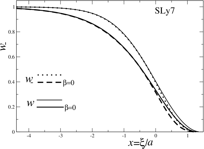
Figure 2: Isovector $w_{-}$ [Eq. (7)] particle density vs $x=\xi/a$ with and without ($\beta=0$) SO terms for the Skyrme force SLy7 as a typical example like in Ref. magsangzh ; the isoscalar $w$ [see Eqs. (3), (A3)] is also shown by solid lines.

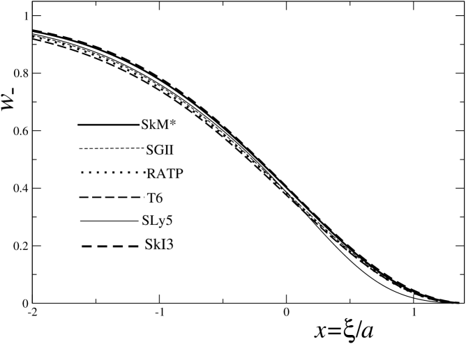
Figure 3: Isovector particle densities $w_{-}(x)$ (7) as functions of $x$ within the quadratic approximation to $\epsilon(w)$ for several Skyrme forces chaban ; reinhard , see also Ref. magsangzh .

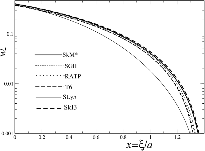
Figure 4: The same as in Fig. 3 for the critical Skyrme interactions but within a smaller edge diffuseness region in the logarithmic scale.

In Fig. 2 the SO dependence of the function $w_{-}(x)$ is compared with that of the density $w(x)$ for the SLy7 force as a typical example magsangzh . It might seem from a brief look at Fig. 3 that the isovector $w_{-}(x)$ [and therefore, the isoscalar $w(x)$] densities depend weakly on the most of the Skyrme forces chaban ; reinhard . However, as shown in a larger (logarithmic) scale in Fig. 4, one observes notable differences in the isovector densities $w_{-}$ derived from different Skyrme forces within the edge diffuseness. In particular, as shown below, this is important for the calculations of the neutron skins of nuclei.

We emphasize that the dimensionless densities, $w(x)$ [Eqs. (3) and (A3) ] and $w_{-}(x)$ [Eq. (7)], shown in Figs. 2-4 were obtained in the leading ES approximation ($a/R\ll 1$) as functions of the specific combinations of the Skyrme force parameters such as $\beta$ and $c_{sym}$ of Eq. (6). Therefore, they are the universal distributions independent of the specific properties of the nucleus such as the neutron and proton numbers, and the deformation and curvature of the nuclear ES; see also Refs. strtyap ; strmagden ; magsangzh . These distributions yield approximately the spatial coordinate dependence of local densities in the direction that is normal to the ES with the correct asymptotical behavior outside of the ES layer for any ES deformation satisfying the condition $a/R\ll 1$ (in particular, for the semi-infinite nuclear matter); see further discussions below.

III Isovector energy and stiffness

Within the improved ES approximation where also higher order corrections in the small parameter $a/R$ are taken into account we derive equations for the nuclear surface itself (see Appendix B and Refs. strmagbr ; strmagden ; magsangzh ). For more exact isoscalar and isovector particle densities we account for the main terms in the next order of the parameter $a/R$ in the Lagrange equations [cf. Eq. (B1) as compared with Eq. (A1)]. Multiplying these equations by $\partial\rho_{-}/\partial\xi$ and integrating them over the ES in the normal-to-surface direction $\xi$ and using the solutions for $w_{\pm}(x)$ up to the leading orders [see Eqs. (3) and (7)], one arrives at the ES equations in the form of the macroscopic boundary conditions (B2) strtyap ; strmagbr ; strmagden ; magsangzh ; kolmagsh ; magstr ; magboundcond ; bormot . They ensure equilibrium through the equivalence of the volume and surface (capillary) pressure (isoscalar or isovector) variations. As shown in Appendix B, the latter ones are proportional to the corresponding surface tension coefficients:

$$\sigma_{\pm}=b_{S}^{(\pm)}/(4\pi r_{0}^{2}),\qquad b_{S}^{(\pm)}\approx 8\pi r_{0}^{2}{\cal C}_{\pm}\int_{-\infty}^{\infty}\hbox{d}\xi\;\left(1+\frac{{\cal D}_{\pm}}{{\cal C}_{\pm}}\rho_{+}\right)\left(\frac{\partial\rho_{\pm}}{\partial\xi}\right)^{2}.$$ (8)

The nuclear energy $E$ [Eq. (1)] in this improved ES approximation (Appendix C) is split into volume and surface (both with the symmetry) terms,

$$E\approx-b_{V}\;A+J(N-Z)^{2}/A+E_{S}\;.$$ (9)

For the surface energy $E_{S}$ one obtains

$$E_{S}=E_{S}^{(+)}+E_{S}^{(-)}$$ (10)

with the following isoscalar (+) and isovector (-) surface components:

$$E_{S}^{(\pm)}=\sigma_{\pm}{\cal S}=b_{S}^{(\pm)}{\cal S}/(4\pi r_{0}^{2}),$$ (11)

where ${\cal S}$ is the surface area of the ES. The energies $E_{S}^{(\pm)}$ in Eq. (11) are determined by the isoscalar $b_{S}^{(+)}$ and isovector $b_{S}^{(-)}$ surface energy constants of Eq. (8). These constants are proportional to the corresponding surface tension coefficients $\sigma_{\pm}$ in Eq. (8) through the solutions (3) and (7) for $\rho_{\pm}(\xi)$ which can be taken into account in leading order of $a/R$ (Appendix C). These coefficients $\sigma_{\pm}$ are the same as those found in the expressions for the capillary pressures of the boundary conditions (B2).

For the energy surface coefficients $b_{S}^{(\pm)}$ one obtains

$$b_{S}^{(+)} = \frac{6{\cal C}_{+}\overline{\rho}{\cal J}_{+}}{r_{0}a},\qquad{\cal J}_{+}=\int_{0}^{1}\hbox{d}w\sqrt{w(1+\beta w)\epsilon(w)}\;,$$ (12)

$$b_{S}^{(-)} = k_{S}\;I^{2},\qquad~{}~{}~{}~{}~{}k_{S}=6\overline{\rho}\;{\cal C}_{-}\;{\cal J}_{-}/(r_{0}a)\;,$$ (13)

$$\vspace{-4ex}{\cal J}_{-} = -\frac{1}{1+\beta}\int_{0}^{1}\left(1-w\right)^{2}\hbox{d}w\;\sqrt{\frac{w(1+\beta w)}{\epsilon(w)}}\;\left(1+\widetilde{c}\widetilde{w}\right)^{2}\;.$$ (14)

For $\widetilde{w}$ and $\widetilde{c}$, see Eqs. (6) and (7), respectively. Simple expressions for the constants $b_{S}^{(\pm)}$ in Eqs. (12) and (13) can be easily derived in terms of algebraic and trigonometric functions by calculating explicitly the integrals over $w$ for the quadratic form of $\epsilon(w)$ [Eqs.  (C3) and (V)]. Note that in these derivations we neglected curvature terms and, being of the same order, shell corrections. The isovector energy terms were obtained within the ES approximation with high accuracy up to the product of two small quantities, $I^{2}$ and $(a/R)^{2}$.

According to the theory myswann69 ; myswnp80pr96 ; myswprc77 , one may define the isovector stiffness $Q$ with respect to the difference $R_{n}-R_{p}$ between the neutron and proton radii as a collective variable,

$$E_{s}^{(-)}=-\frac{\overline{\rho}r_{0}}{3}\oint\hbox{d}S\;Q\tau^{2}\approx-\frac{Q\tau^{2}{\cal S}}{4\pi r_{0}^{2}},\qquad\tau=\frac{R_{n}-R_{p}}{r_{0}}\;,$$ (15)

where $\tau$ is the neutron skin. Comparing this expression with Eq. (11) for the isovector surface energy written through the isovector surface energy constant $b_{S}^{(-)}$ [Eq. (13)], one obtains

$$Q=-b_{S}^{(-)}/\tau^{2}=-k_{S}I^{2}/\tau^{2}\;.$$ (16)

Defining the neutron and proton radii $R_{n,p}$ as the positions of the maxima of the neutron and proton density gradients, respectively,

$$\left(\frac{\partial^{2}\rho_{n,p}}{\partial r^{2}}\right)_{r=R_{n,p}}=0,\qquad\left(\frac{\partial^{2}\rho_{+}}{\partial r^{2}}\right)_{r=R}=0,$$ (17)

we use the expansion in small values of $\delta R_{n,p}=R_{n,p}-R$ near the ES. Thus, in the linear approximation in $\delta R_{n,p}$ and $I$ one obtains

$$\tau=-2\frac{aI}{r_{0}}\;\frac{\partial^{2}w_{-}}{\partial x^{2}}\Big{|}_{x=0}\left(\frac{\partial^{3}w}{\partial x^{3}}\Big{|}_{x=0}\right)^{-1}=\frac{8aI}{r_{0}c_{sym}^{2}}g(w_{r}),\,$$ (18)

where

$$g(w)=\frac{w^{3/2}(1+\beta w)^{5/2}}{(1+\beta)(3w+1+4\beta w)}\;\left\{w(1+2\widetilde{c}\widetilde{w})^{2}+2\widetilde{w}\left(1+\widetilde{c}\widetilde{w}\right)\left[\widetilde{c}w-c_{sym}\left(1+2\widetilde{c}\widetilde{w}\right)\right]\right\},$$ (19)

and $w_{r}$ is the solution of the boundary equation (4). In the derivations of Eq. (18), we used the approximation $\epsilon(w)=(1-w)^{2}$ and expressions (3) for $w(x)$ and (7) for $w_{-}(x)/w$. The neutron and proton particle-density variations in Eq. (17) conserve the center of mass in the same linear approximation in $\delta R_{n,p}$ and $I$. Inserting Eqs. (18) and (13) into Eq. (16), one finally arrives at

$$Q=-\nu\;\frac{J^{2}}{k_{S}},\qquad\nu=\frac{k_{S}^{2}I^{2}}{\tau^{2}J^{2}}=\frac{9{\cal J}_{-}^{2}}{16g^{2}(w_{r})}\;,$$ (20)

where ${\cal J}_{-}$ and $g(w_{r})$ are given by Eqs. (14), (19), and (4). In the derivation of Eq. (20) we used also Eq. (3) for the diffuseness parameter $a$ and Eq. (6) for $c_{sym}$. Note that $Q=-9J^{2}/4k_{S}$ has been predicted in Refs. myswann69 ; myswnp80pr96 and therefore for $\nu=9/4$ the first part of (20), which relates $Q$ with the volume symmetry energy $J$ and the isovector surface energy $k_{S}$ constants, is identical to that used in Refs. myswann69 ; myswnp80pr96 ; myswprc77 ; myswiat85 ; vinas1 ; vinas2 . However, in our derivations $\nu$ deviates from $9/4$ and it is proportional to the function ${\cal J}_{-}^{2}/g^{2}(w_{r})$. This function depends significantly on the SO interaction parameter $\beta$ but not too much on the specific Skyrme forces. Indeed, the most sensitive parameter ${\cal C}_{-}$ cancels in the expression (20) for $\nu$: $k_{S}\propto{\cal C}_{-}$ and $\tau\propto 1/c_{sym}^{2}\propto{\cal C}_{-}$ [see also Eqs.  (13) for $k_{S}$, (6) for $c_{sym}$ and (18) for $\tau$]. The constant $\nu$ at $\beta=0$ can be easy evaluated,

$$\nu\approx\frac{108}{25}\;\frac{\left[1-8/(7c_{sym})\right]^{2}}{1-4/(3c_{sym})},$$ (21)

neglecting small terms $\propto 1/c_{sym}^{2}$, $c_{sym}\approx 2-6$, for the Skyrme parameters of Refs. chaban ; reinhard [$c_{sym}=\infty$ for T6 forces; see Eqs. (20), (14), (6), and (4) ($w_{r}=1/3$) and Table I]. Another difference in $Q$ [ Eq. (20)] from that of Refs. myswann69 ; myswnp80pr96 ; myswprc77 ; myswiat85 is the expression (13) itself for $k_{S}$. Thus, the isovector stiffness coefficient $Q$ introduced originally by Myers and Swiatecki myswann69 ; myswnp80pr96 is not a parameter of our approach but was found analytically in the explicit closed form (20) through the parameters of the Skyrme forces.

Notice that the universal functions $w(x)$ [Eqs. (3) and (A3) ] and $w_{-}(x)$ [Eq. (7)] of the leading order in the ES approximation can be used [explicitly analytically in the quadratic approximation for $\epsilon(w)$] for the calculations of the surface energy coefficients $b_{S}^{(\pm)}$ [Eq. (8)] and the neutron skin $\tau$ [Eq. (18)]. As shown in Appendixes B and C, only these particle-density distributions $w(x)$ and $w_{-}(x)$ within the surface layer are needed through their derivatives [the lower limit of the integration over $\xi$ in Eq. (8) can be approximately extended to $-\infty$ because of no contributions from the internal volume region in the evaluation of the main surface terms of the pressure and energy]. Therefore, the surface symmetry-energy coefficient $k_{S}$ in Eqs. (13) and (V) , the neutron skin $\tau$ [Eq. (18)], and the isovector stiffness $Q$ [Eq. (20)] can be approximated analytically in terms of the functions of the definite critical combinations of the Skyrme parameters such as $\beta$, $c_{sym}$, $a$, and the parameters of the infinite nuclear matter ($b_{V},\overline{\rho},K$). Thus, they are independent of the specific properties of the nucleus (for instance, the neutron and proton numbers), and the curvature and deformation of the nuclear surface in the considered ES approximation.

IV Discussion of the results

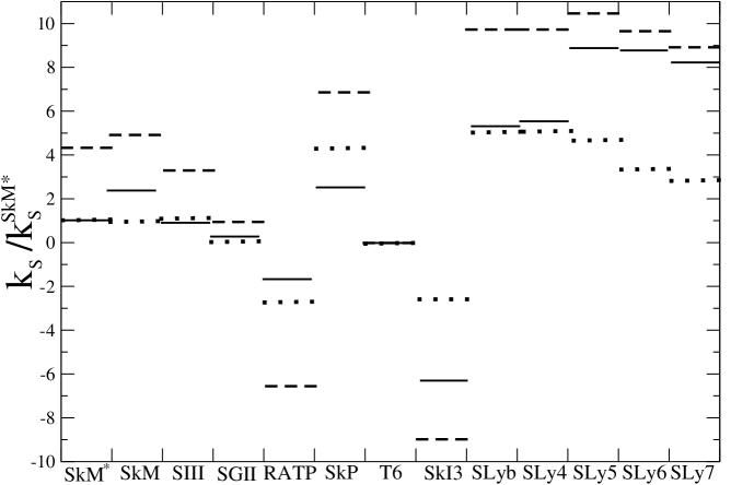
Figure 5: Isovector energy constant $k_{S}$ of Eq. (13) (solid bars) vs the coefficient ${\cal C}_{-}$ (dotted points) of Eq. (2) normalized both by their values $k_{S}^{SkM^{*}}$ and ${\cal C}_{-}^{SkM^{*}}$ for the Skyrme force SkM^∗, respectively; $k_{s,0}$ (dashed bars) in the same units $k_{S}^{SkM^{*}}$ is given by Eq. (13) without the spin-orbit interaction ($\beta=0$).

In Table II and also in Fig. 5 we show the isovector energy coefficient $k_{S}$ [Eq. (13)], the stiffness parameter $Q$ [Eq. (20)], and the neutron skin $\tau$ [Eq. (18)] obtained within the ES approximation using the quadratic approximation for $\epsilon(w)$ for several Skyrme forces chaban ; reinhard with parameters presented in Table I. We also show the quantities $k_{S\;0}$, $\nu_{0}$, $Q_{0}$ and $\tau_{0}$ where the SO interaction is neglected ($\beta=0$). One can see a fairly good agreement for the analytical isoscalar energy constant $b_{S}^{(+)}$ (12) with that of Refs. chaban ; reinhard and magsangzh (Table I). The isovector energy coefficient $k_{S}$ is more sensitive to the choice of the Skyrme forces than the isoscalar one $b_{S}^{(+)}$ (Eq. (12) and Ref. magsangzh ). The modulus of $k_{S}$ is significantly larger for most of the Lyon Skyrme forces SLy chaban and SkI3 reinhard than for the other ones. For these forces the stiffnesses $Q$ are correspondingly smaller. The isovector stiffness $Q$ is even more sensitive to the constants of the Skyrme force than the constants $k_{S}$. They are significantly larger for all forces, especially for SGII, than the well known empirical values $Q\approx 14-35$ MeV myswprc77 ; myswnp80pr96 ; myswiat85 .

Swiatecki and his collaborators myswprc77 found the stiffness $Q\approx 14-20$ MeV by fitting the nuclear isovector giant dipole-resonance (IVGDR) energies calculated in the simplest version of the hydrodynamical model to the experimental data. Later, they suggested larger values $Q\approx 30-35$ MeV accounting for a more detailed study of other phenomena in Refs. myswnp80pr96 ; myswiat85 . In spite of several misprints in the derivations of the IVGDR energies in Ref. myswprc77 (in particular, in Eq. (7.7) of myswprc77 for the displacement of the center-of-mass conservation, the factor $NZ/A^{2}$ should be in the numerator and not in the denominator of the irrotational flow moment of inertia; see Ref. eisgrei )), the final result for the IVGDR energy constant is almost the same as for the asymptotically large values of $Q$, $3JA^{-1/3}/Q\ll 1$ ($NZ/A^{2}\approx 1/4$),

$$D=\hbar\omega_{-}A^{1/3}=D_{\infty}/\sqrt{1+3JA^{-1/3}/Q},\qquad D_{\infty}=\sqrt{8\hbar^{2}J/\left(mr_{0}^{2}\right)}\;.$$ (22)

These values for $D$ are in good agreement with the well known experimental value $D_{exp}\approx 80$ MeV for heavy nuclei ($D\approx D_{\infty}\approx 88$ MeV) within a precision better than or of the order of 20% (a little worse for the specific SkI3 Skyrme forces), as shown in Table II, see also Ref. denisov for a more proper HD approach and Refs. plujko1 ; plujko2 ; plujko3 for other semiclassical nuclear models taking all into account the nuclear surface motion. As shown in Ref. BMV , the averaged IVGDR energies and the energy weighted sum rules (EWSR), obtained with the semiclassical FLD approach based on the Landau-Vlasov equation kolmagsh with macroscopic boundary conditions (see Appendix B), are also basically insensitive to the isovector surface energy constant $k_{S}$, and they are similarly in good agreement with the experimental data. An investigation of the splitting of the IVGDR within this approach into the main peak which exhausts mainly the independent-of-model EWSR and a satellite (with a much smaller contribution to the EWSR), focusing on a much more sensitive $k_{S}$ dependence of the pygmy (IVGDR satellite) resonances (see Refs. kievPygmy ; nester ), will be published elsewhere.

More precise $A$ dependence of the quantity $D$ [Eq. (22)] for finite values of $Q$ seems to be beyond the accuracy of these HD calculations because of several other reasons. More realistic self-consistent HF calculations accounting for the Coulomb interaction, surface-curvature, and quantum-shell effects led to larger $Q\approx 30-80$ MeV brguehak ; vinas2 . With larger $Q$ (see Table II) the fundamental parameter of the LDM expansion in Ref. myswann69 , $(9J/4Q)A^{-1/3}$, is really small for $A\hbox{\kern 1.00006pt\lower 2.58334pt\hbox{$\sim$} \kern-11.19997pt\raise 2.58334pt\hbox{$>$} \kern 1.00006pt}40$, and therefore results obtained by using this expansion are more justified.

The most responsible parameter of the Skyrme HF approach leading to significant differences in the $k_{S}$ and $Q$ values is the constant ${\cal C}_{-}$ in the gradient terms of the energy density [Eq. (2) and Table I]. Indeed, the key quantity in the expression for $Q$, Eq. (20), and the isovector surface energy constant $k_{S}$ [or $b_{S}^{(-)}$, Eq. (13)], is the constant ${\cal C}_{-}$ because one mainly has $k_{S}\propto{\cal C}_{-}$ (see Fig. 5), and $Q\propto 1/k_{S}\propto 1/{\cal C}_{-}$. As seen in Table I and in Fig. 5 the constant ${\cal C}_{-}$ is very different for the different Skyrme forces (even in sign). As shown in Fig. 3 and below Eq. (20), other quantities in Eq. (20) are much less sensitive to most Skyrme interactions. The situation is very much in contrast to the isoscalar energy density constant $b_{S}^{(+)}\propto C_{+}$ [Eq. (12)]. All Skyrme parameters are fitted to the well known experimental value $b_{S}^{(+)}=17-19$ MeV because ${\cal C}_{+}$ is almost constant (Table I). Contrary to this, there are so far no clear experiments which would determine $k_{S}$ well enough because the mean energies of the IVGDR (main peaks) do not depend very much on $k_{S}$ for the different Skyrme forces (see last two rows of Table II). Perhaps, the low-lying isovector collective states are more sensitive but there is no careful systematic study of their $k_{S}$ dependence at the present time. Another reason for such different $k_{S}$ and $Q$ values might be traced back to the difficulties in deducing $k_{S}$ directly from the HF calculations due to the curvature and quantum effects, in contrast to $b_{S}^{(+)}$. We also have to go far away from the nuclear stability line to subtract uniquely the coefficient $k_{S}$ in the dependence of $b_{S}^{(-)}\propto I^{2}=(N-Z)^{2}/A^{2}$, according to Eq. (13). For exotic nuclei one has more problems to relate $k_{S}$ to the experimental data with a good enough precision. Note that $k_{S}$ is a more fundamental constant than the isovector stiffness $Q$ due to the direct relation to the tension coefficient $\sigma_{-}$ of the isovector capillary pressure. Therefore, it is simpler to analyze the experimental data for the IVGDR within the macroscopic HD or FLD models in terms of the constant $k_{S}$. The quantity $Q$ involves also the ES approximation for the description of the nuclear edge through the neutron skin $\tau$ [see Eq. (15)]. The precision of this description depends more on the specific nuclear models vinas1 ; vinas2 ; vinas3 ; vinas4 . On the other hand, the neutron skin thickness $\tau$ is interesting in many aspects for the investigation of exotic nuclei, in particular, in nuclear astrophysics.

We emphasize that for specific Skyrme forces there exists an abnormal behavior of the isovector surface constants $k_{S}$ and $Q$. It is related to the fundamental constant ${\cal C}_{-}$ of the energy density (2). For the parameter set T6 (${\cal C}_{-}=0$) one finds $k_{S}=0$. Therefore, according to Eq. (20), the value of $Q$ diverges ($\nu$ is almost independent on ${\cal C}_{-}$). Notice that the isovector gradient terms which are important for the consistent derivations within the ES approach are also not included (${\cal C}_{-}=0$) in the symmetry energy density in Refs. danielewicz1 ; danielewicz2 . Moreover, for RATP chaban and SkI reinhard (also for the specific Skyrme forces BSk6 and BSk8 of Ref. pearson ), the isovector stiffness $Q$ is even negative as ${\cal C}_{-}>0$ ($k_{S}>0$), in contrast to all other Skyrme forces.

Table II shows also the coefficients $\nu$ of Eq. (20) for the isovector stiffness $Q$. They are mostly constant [$\nu_{0}\approx 2-4$; see Eq. (21) and Table II] for all Skyrme forces at $\beta=0$. However, these constants $\nu$ are rather sensitive to the SO interaction, i.e., to the $\beta$ dependence of both the function $g(w_{r})$ [Eq. (19)] in expression (18) for the neutron skin $\tau$ and to the constant ${\cal J}_{-}$ [Eq. (14)] in expression (13) for the isovector energy coefficient $k_{S}$. As compared to 9/4 suggested in Ref. myswann69 , they are significantly smaller in magnitude for the most of the Skyrme forces (besides those of SGII and T6 with larger values of $\nu$).

V Conclusions

Simple expressions for the isovector parts of the particle densities and energies in the leading ES approximation were used for the derivation of analytical expressions of the surface symmetry energy, the neutron skin thickness, and the isovector stiffness coefficients. As shown in Appendix B we have to include higher order terms in the parameter $a/R$. These terms depend on the well known parameters of the Skyrme forces. Results for the isovector surface energy constant $k_{S}$, the neutron skin thickness $\tau$, and the stiffness $Q$ depend in a sensitive way on the choice of the parameters for the Skyrme functional, especially on the parameter ${\cal C}_{-}$ in the gradient terms of the density in the surface symmetry energy density of Eq. (2). The values of the isovector constants $k_{S}$, $\tau$, and $Q$ depend also very much on the SO interaction constant $\beta$. The isovector stiffness constants $Q$ are significantly larger than those found earlier for all desired Skyrme forces. The mean IVGDR energies and sum rules calculated in the HD myswprc77 ; denisov ; eisgrei and FLD kolmagsh ; BMV models for most of the $k_{S}$ values in Table II are in a fairly good agreement with the experimental data. For further perspectives, it would be worthwhile to apply our results to the calculations of the pygmy resonances in the IVGDR strength within the FLD model kolmagsh and the isovector low-lying collective states within the periodic orbit theory gzhmagfed ; blmagyas ; BM , which are expected to be more sensitive to the values of $k_{S}$. Our approach is helpful for further study of the effects in the surface symmetry energy because it gives the analytical universal expressions for the constants $k_{S}$, $\tau$ and $Q$ which are independent of the specific properties of the nucleus. These constants are directly connected with a few critical parameters of the Skyrme interaction without using any fitting.

Acknowledgements

The authors thank M. Brack, M. Brenna, V.Yu. Denisov, V.M. Kolomietz, J. Meyer, V.O. Nesterenko, M. Pearson, V.A. Plujko, X. Roca-Maza, A.I. Sanzhur, and X. Vinas for many useful discussions. One of us (A.G.M.) is also very grateful for hospitality during his working visits to the National Centre for Nuclear Research in Otwock-Swierk of Poland. This work was partially supported by the Deutsche Forschungsgemeinschaft Cluster of Excellence Origin and Structure of the Universe (www.universe-cluster.de).

Appendix A: Solutions to the isovector Lagrange equation

The Lagrange equation for the variations of the isovector particle density $\rho_{-}$ in the energy density (2) up to the leading terms in a small parameter $a/R$ is given by magsangzh

$${\cal C}_{-}\;\frac{\partial^{2}\rho_{-}}{\partial\xi^{2}}+\frac{\hbox{d}}{\hbox{d}\rho_{-}}\left[\rho_{+}\varepsilon_{-}(\rho_{+},\rho_{-})\right]=0,$$ (A1)

where $\varepsilon_{-}$ is defined just below Eq. (2). We neglected here the higher order terms proportional to the first derivatives of the particle density $\rho_{-}$ with respect to $\xi$ and the surface correction to the isovector chemical potential as in Refs. strmagbr ; strmagden for the isoscalar case. For the dimensionless isovector density $w_{-}=\rho_{-}/(\overline{\rho}I)$, after simple transformations one finds the equation and the boundary condition in the form

$$\frac{\hbox{d}w_{-}}{\hbox{d}w}=c_{sym}\sqrt{\frac{1+\beta w}{\epsilon(w)}}\;\sqrt{1-\frac{w_{-}^{2}}{w^{2}}},\qquad w_{-}(1)=1\;,$$ (A2)

where $\beta$ is the SO parameter defined below Eq. (3); see also Eq. (6) for $c_{sym}$. The above equation determines the isovector density $w_{-}$ as a function of the isoscalar one $w(x)$ [Eq. (3)]. In the quadratic approximation for $\epsilon(w)$ one explicitly finds

$$x(w) = \sqrt{1+\beta}\,\ln\left[\frac{(1-w)\left(1+(1+2\beta)w_{r}+2\sqrt{(1+\beta)(1+\beta w_{r})w_{r}}\right)}{(1-w_{r})\left(1+(1+2\beta)w+2\sqrt{(1+\beta)(1+\beta w)w}\right)}\right]$$ (A3)

$$+ \sqrt{-\beta}\left[\arcsin\left(1+2\beta w\right)-\arcsin\left(1+2\beta w_{r}\right)\right]\;,\qquad x<x(w=0)$$

and $w=0$ for $x\geq x(w=0)$; $w_{r}$ is the solution of the boundary condition (4). Substituting $w_{-}=w\;\hbox{cos}\psi$ into Eq. (A2), and taking the approximation $\epsilon=(1-w)^{2}$, one has the following first order differential equation for a new function $\psi(w)$:

$$\frac{w(1-w)}{c_{sym}}\;\hbox{sin}\psi\;\frac{\hbox{d}\psi}{\hbox{d}w}=\sqrt{1+\beta w}\;\hbox{sin}\psi-\frac{1-w}{c_{sym}}\;\hbox{cos}\psi,\qquad\qquad\psi(1)=0.$$ (A4)

The boundary condition for this equation is related to that of Eq. (A2) for $w_{-}(w)$. This equation looks more complicated because of the trigonometric nonlinear terms. However, it allows us to obtain simple approximate and rather exact analytical solutions within standard perturbation theory. Indeed, according to Eqs. (A2) and (3) where we did not express the $x$ dependence explicitly, we note that $w_{-}\propto w(x)$ is a sharply decreasing function of $x$ within a small diffuseness region of the order of 1 in dimensionless units (Figs. 2-4). Thus, we may find the approximate solutions to the equation (A4) (with its boundary condition), in terms of a power expansion of a new function $\widetilde{\psi}(\widetilde{w})$ in terms of a new small argument $\widetilde{w}$,

$$\widetilde{\psi}(\widetilde{w})\equiv\psi(w)=\sum_{n=0}^{\infty}c_{n}\;\widetilde{w}^{n}\;,$$ (A5)

with unknown coefficients $c_{n}$ and $\widetilde{w}$ defined in Eq. (6). Substituting the power series (A5) into Eq. (A4) one expands first the trigonometric functions into power series of $\widetilde{w}$ in accordance with the boundary condition in Eq. (A4). As usual, using standard perturbation theory, we obtain the system of algebraic equations for the coefficients $c_{n}$ [Eq. (A5)] by equating the coefficients from both sides of Eq. (A4) at the same powers of $\widetilde{w}$. This simple procedure leads to a system of algebraic recurrence relations which determine the coefficients $c_{n}$ as functions of the parameters $\beta$ and $c_{sym}$ of Eq. (A4),

$$c_{0} = 0,\qquad\qquad c_{1}=\frac{1}{\sqrt{1+\beta}},\qquad\qquad c_{2}=\frac{c_{1}}{\sqrt{1+\beta}}\left(\frac{\beta c_{sym}}{2\sqrt{1+\beta}}-c_{1}\right),$$

$$c_{3} = \frac{1}{\sqrt{1+\beta}}\left\{\frac{\beta^{2}c_{sym}^{2}c_{1}}{8\left(1+\beta\right)^{3/2}}+c_{1}^{2}\left(c_{sym}-\frac{1}{2}\right)+\frac{1}{6}\sqrt{1+\beta}c_{1}^{3}+c_{2}\left(\frac{\beta c_{sym}}{2\sqrt{1+\beta}}-3c_{1}\right)\right\},$$ (A6)

etc. In particular, up to the second order in $\widetilde{w}$, we derive an analytical solution in an explicitly closed form:

$$\widetilde{\psi}(\widetilde{w})=\widetilde{w}\left(c_{1}+c_{2}\widetilde{w}\right),\quad c_{1}=\frac{1}{\sqrt{1+\beta}},\quad c_{2}=\frac{1}{(1+\beta)^{3/2}}\left(\frac{\beta}{2}c_{sym}-1\right).$$ (A7)

Thus, using the standard perturbation expansion method of solving $\widetilde{\psi}(\widetilde{w})$ in terms of the power series of the $\widetilde{w}$ (up to $\widetilde{w}^{2}$), one obtains the quadratic expansion of $\psi(w)$ [Eq. (7)] with $\widetilde{c}=c_{2}/c_{1}$. Notice that one finds a good convergence of the power expansion of $\widetilde{\psi}(\widetilde{w})$ (A7) in $\widetilde{w}$ for $w_{-}(x)$ at the second order in $\widetilde{w}$ because of the large value of $c_{sym}$ for all Skyrme forces presented in Table I [Eq. (6) for $c_{sym}$].

Appendix B: The macroscopic boundary conditions and surface tension coefficients

For the derivation of the expression for the surface tension coefficients $\sigma_{\pm}$, we first write the system of the Lagrange equations by using variations of the energy density ${\cal E}(\rho_{+},\rho_{-})$ with respect to the isoscalar and isovector densities $\rho_{+}$ and $\rho_{-}$. Then, we substitute the solution of the first Lagrange equation for the variations of the isoscalar density $\rho=\rho_{+}$ in the energy density (2) (Refs. strmagbr ; strmagden ) into the second Lagrange equation for the isovector density $\rho_{-}$. Using the Laplacian in the variables $\xi$ and $\eta$ (Appendix A in Ref. strmagbr ) we keep the major terms in this second equation within the improved precision in the small parameter $a/R$. The improved precision means that we take into account the next terms proportional to the first derivatives of the particle densities [along with the second ones of Eq. (A1)] and the small surface corrections $\Lambda_{\pm}$ to the isoscalar and isovector Lagrange multipliers $\lambda_{\pm}$. Within this improved precision, one finds the second Lagrange equation by the variations of the energy density ${\cal E}(\rho_{+},\rho_{-})$, Eq. (2), with respect to the isovector particle density $\rho_{-}$:

$${\cal C}_{-}\;\frac{\partial^{2}\rho_{-}}{\partial\xi^{2}}+2{\cal C}_{-}H\frac{\partial\rho_{-}}{\partial\xi}-\frac{\hbox{d}}{\hbox{d}\rho_{-}}\left[\rho_{+}\varepsilon_{-}(\rho_{+},\rho_{-})\right]+\Lambda_{-}=0,$$ (B1)

where $H$ is the mean curvature of the ES ($H=1/R$ for the spherical ES). The isovector chemical-potential correction $\Lambda_{-}$ was introduced magsangzh like the isoscalar one $\Lambda_{+}$, worked out in detail in Refs. strmagbr ; strmagden . Multiplying Eq. (B1) by $\partial\rho_{-}/\partial\xi$ we integrate in the coordinate $\xi$ normal to the ES from a spatial point $\xi_{in}$ inside the volume (at $\xi_{in}\hbox{\kern 1.00006pt\lower 2.58334pt\hbox{$\sim$} \kern-11.19997pt\raise 2.58334pt\hbox{$<$} \kern 1.00006pt}-a$ ) to $\infty$ term by term. Using also integration by parts, within the ES approximation this results in the macroscopic boundary conditions (together with the isoscalar condition from strmagbr ; strmagden ; magsangzh ; kolmagsh ; magstr ; magboundcond )

$$\left(\overline{\rho}\;I\;\Lambda_{-}\right)_{ES}=P_{s}^{(-)}\equiv 2\sigma_{-}H,\qquad\left(\overline{\rho}\;\Lambda_{+}\right)_{ES}=P_{s}^{(+)}\equiv 2\sigma_{+}H.$$ (B2)

Here, $P_{s}^{(\pm)}$ are the isovector and isoscalar surface-tension (capillary) pressures and $\sigma_{\pm}$ are the corresponding tension coefficients; see their expressions in Eq. (8). We point out that the lower limit $\xi_{in}$ can be approximately extended to $-\infty$ as in Eq. (8) for $\sigma_{\pm}$. The integrands contain the square of the first derivatives, $(\partial\rho_{\pm}/\partial\xi)^{2}\propto(R/a)^{2}$, and the integral over $\xi$ converges exponentially rapidly within the ES layer $|\xi|\leq a$. This leads to the aditional small factor $a/R$ in Eq. (8), $\sigma_{\pm}\propto R/a$. Therefore, at this higher order of the improved ES approximation one may neglect higher order corrections in the calculation of derivatives of $\rho_{\pm}$ themselves by using the analytical universal density distributions $w_{\pm}(x)$ [Eqs. (3), (A3) and (7)] within the ES layer which do not depend on the specific properties of the nucleus as mentioned in the main text. (These corrections are small terms proportional to the first derivative $\partial\rho_{-}/\partial\xi$ and $\Lambda_{-}$ in Eq. (B1), as for the isoscalar case considered in Refs. strmagbr ; strmagden ; magstr ; magboundcond ). In these derivations, the obvious boundary conditions of disappearance of the particle densities and all their derivatives with respect to $\xi$ outside of the ES for $\xi\rightarrow\infty$ ($\xi\gg a$) were taken into account too.

The Lagrange multipliers $\Lambda_{\pm}$ multiplied by $\overline{\rho}I$ and $\overline{\rho}$ in the parentheses on the left-hand sides of equations (B2) are the volume isovector ($\overline{\rho}I\Lambda_{-}$) and isoscalar ($\overline{\rho}\Lambda_{+}$) pressure excesses, respectively (see Ref. magsangzh ). These pressures due to the surface curvature can be derived using the volume solutions of the Lagrange equations for the particle densities [obtained by doing variations of the energy density ${\cal E}$ and neglecting all the derivatives of the particle densities in Eq. (2)],

$$\rho_{-}\approx\overline{\rho}\;\left[I\left(1+\frac{9\Lambda_{+}}{K}\right)+\frac{\Lambda_{-}}{2J}\right],\quad\rho_{+}\approx\overline{\rho}\left[1+\frac{9\Lambda_{+}}{K}\left(1-\frac{81\Lambda_{+)}}{2K}\right)-\frac{18J}{2K}\;I^{2}\right]\;.$$ (B3)

Inserting $\Lambda_{+}$ and $\Lambda_{-}$ from Eq. (B2) into Eq. (B3) one gets

$$\rho_{-}=\overline{\rho}\;I\;\left[1+\frac{6b_{S}^{(+)}\;H\;r_{0}}{K}+\frac{2b_{S}^{(-)}\;H\;r_{0}}{6J\;I^{2}}\right].$$ (B4)

As seen from Eq. (B4), the isovector density correction to the volume density $\rho_{-}$ due to a finiteness of the coupled system of the two Lagrange equations depends on both isoscalar and isovector surface energy constants $b_{S}^{(\pm)}$ in the first-order expansion of the small parameter $a/R$. If we are not too far from the valley of stability $I$ is an additional small parameter and the isovector corrections are small compared with the isoscalar values [$b_{S}^{(-)}\propto I^{2}$, $\Lambda_{-}\propto I$; see Eqs. (B3), (B4), and (13)]. Thus, Eq. (B2) has a clear physical meaning as the macroscopic boundary conditions for equilibrium of the isovector and isoscalar forces (volume and surface pressures) acting on the ES bormot ; kolmagsh . Note that the isovector tension coefficient $\sigma_{-}$ is much smaller than the isoscalar one $\sigma_{+}$ [see Eq. (8)] as $\sigma_{-}\propto I^{2}$ due to $\rho_{-}\propto I$ and $I\ll 1$ is small near the nuclear stability line. Another reason is the smallness of ${\cal C}_{-}$ as compared to ${\cal C}_{+}$ for the realistic Skyrme forces chaban ; reinhard . From comparison of Eqs. (B3) and (B4) for $\rho_{-}$ [see also Eq. (8)], one may also evaluate

$$\Lambda_{-}=\frac{2\sigma_{-}H}{\overline{\rho}\;I}\approx\frac{2b_{S}^{(-)}}{3IA^{1/3}}\sim k_{S}I\frac{a}{R}\;.$$ (B5)

which is consistent with Eq. (B1) ($r_{0}H\sim a/R$ in these estimations, see corresponding ones in Refs. strmagbr ; strmagden ).

Appendix C: Derivations of the surface energy and its coefficients

For calculations of the surface energy components $E_{S}^{(\pm)}$ of the energy $E$, Eq. (1), within the same improved ES approximation as described above in Appendix B, we first may separate the volume terms related to the first two terms of Eq. (2) for the energy density ${\cal E}$. Other terms of the energy density ${\cal E}(\rho_{+},\rho_{-})$ in Eq. (2) lead to the surface components $E_{S}^{\pm}$ [Eq. (11)], as they are concentrated near the ES. Integrating the energy density ${\cal E}$ [see Eq. (2)] over the spatial coordinates ${\bf r}$ in the local coordinate system $\xi,\eta$ (see Fig. 1) in the ES approximation, one finds

$$E_{S}^{(\pm)}={\cal C}_{\pm}\oint\hbox{d}{\cal S}\int_{\xi_{in}}^{\infty}\hbox{d}\xi\left[\left(\nabla\rho_{\pm}\right)^{2}-\rho_{+}\varepsilon_{\pm}\left(\rho_{+},\rho_{-}\right)\right]\approx\sigma_{\pm}\;{\cal S}\;,$$ (C1)

where $\xi_{in}\hbox{\kern 1.00006pt\lower 2.58334pt\hbox{$\sim$} \kern-11.19997pt\raise 2.58334pt\hbox{$<$} \kern 1.00006pt}-a$ is as in Appendix B strmagbr ; strmagden ; magsangzh . The local coordinates $\xi,\eta$ were used because the integral over $\xi$ converges rapidly within the ES layer which is effectively taken for $|\xi|\hbox{\kern 1.00006pt\lower 2.58334pt\hbox{$\sim$} \kern-11.19997pt\raise 2.58334pt\hbox{$<$} \kern 1.00006pt}a$. Therefore, again, we may extend formally $\xi_{in}$ to $-\infty$ in the first (internal) integral taken over the ES in the normal direction $\xi$ in Eq. (C1). Then, the second integration is performed over the closed surface of the ES. The integrand over $\xi$ contains terms of the order of $(\overline{\rho}/a)^{2}\propto(R/a)^{2}$ as the ones of the leading order in Eq. (B1) [see for instance the second derivatives in Eq. (A1) which are also $\propto(R/a)^{2}$]. However, the integration is effectively performed over the edge region of the order of $a$ that leads to the additional smallness proportional to $a/R$ as in Appendix B. At this leading order the $\eta$ dependence of the internal integrand can be neglected. Moreover, from the Lagrange equations at this order one can realize that the terms without the particle density gradients in Eq. (C1) are equivalent to the gradient terms. Therefore, for the calculation of the internal integral we may approximately reduce the integrand over $\xi$ to the only derivatives of the universal particle densities of the leading order $\rho_{\pm}(\xi)$ in $\xi$ (with the factor 2) using $\left(\nabla\rho_{\pm}\right)^{2}-\rho_{+}\varepsilon_{\pm}\left(\rho_{+},\rho_{-}\right)\approx 2(\partial\rho_{\pm}/\partial\xi)^{2}$ [see Eqs. (3) and (7) for $w_{\pm}(x)$] . Taking the integral over $\xi$ within the infinite integration region ($-\infty<\xi<\infty$) off the integral over the ES ($\hbox{d}{\cal S}$) we are left with the integral over the ES itself that is the surface area ${\cal S}$. Thus, we arrive finally at the right-hand side of Eq. (C1) with the surface tension coefficient $\sigma_{\pm}$ [Eq. (8)].

Using now the quadratic approximation $\epsilon(w)=(1-w)^{2}$ in Eq. (8) for $b_{S}^{(\pm)}=4\pi r_{0}^{2}\sigma_{\pm}$ ($|{\cal D}_{-}/{\cal D}_{+}|\ll 1$), one obtains (for $\beta<0$, see Table I)

$$b_{S}^{(\pm)}=6\overline{\rho}\;{\cal C}_{\pm}\;{\cal J}_{\pm}/(r_{0}a)\;,$$ (C2)

where

$${\cal J}_{+} = \int_{0}^{1}\hbox{d}w\;\sqrt{w(1+\beta w)}\;(1-w)=\frac{1}{24}\;(-\beta)^{-5/2}\;\left[{\cal J}_{+}^{(1)}\;\sqrt{-\beta(1+\beta)}\right.$$ (C3)

$$+ \left.{\cal J}_{+}^{(2)}\;\arcsin\sqrt{-\beta}\right],\qquad{\cal J}_{+}^{(1)}=3+4\beta(1+\beta),\qquad{\cal J}_{+}^{(2)}=-3-6\beta\;.$$

For the isovector energy constant ${\cal J}_{-}$ one finds

$${\cal J}_{-} = -\frac{1}{1+\beta}\;\int_{0}^{1}\hbox{d}w\;\sqrt{w(1+\beta w)}\;(1-w)(1+\widetilde{c}\widetilde{w})^{2}$$

$$= \frac{\widetilde{c}^{2}}{1920(1+\beta)(-\beta)^{9/2}}\;\left[{\cal J}_{-}^{(1)}\left(c_{sym}/\widetilde{c}\right)\;\sqrt{-\beta(1+\beta)}+{\cal J}_{-}^{(2)}\left(c_{sym}/\widetilde{c}\right)\;\arcsin\sqrt{-\beta}\right],$$

$${\cal J}_{-}^{(1)}(\zeta) = 105-4\beta\left\{95+75\zeta+\beta\left[119+10\zeta(19+6\zeta)+8\beta^{2}\left(1+10\zeta(1+\zeta)\right)\right.\right.$$

$$+ \left.\left.8\zeta\left(5\zeta(3+2\zeta)-6\right)\right]\right\},$$

$${\cal J}_{-}^{(2)}(\zeta) = 15\left\{7+2\beta\left[5(3+2\zeta)+8\beta(1+\zeta)\left(3+\zeta+2\beta(1+\zeta)\right)\right]\right\}.$$ (C4)

These equations determine explicitly the analytical expressions for the isoscalar ($b_{S}^{(+)}$) and isovector ($b_{S}^{(-)}$) energy constants in terms of the Skyrme force parameters; see Eqs. (7) for $\widetilde{c}$, (6) for $c_{sym}$ and $\widetilde{w}$. For the limit $\beta\rightarrow 0$ from Eqs. (C3) and (V) one has ${\cal J}_{\pm}\rightarrow 4/15$. With Eqs. (18) and (19) one arrives also at the explicit analytical expression for the isovector stiffness $Q$ as a function of ${\cal C}_{-}$ and $\beta$. In the limit ${\cal C}_{-}\rightarrow 0$ one obtains $k_{S}\rightarrow 0$ and $Q\rightarrow\infty$ because of the finite limit of the argument $c_{sym}/\widetilde{c}\rightarrow(1+\beta)/\beta$ of the function ${\cal J}_{-}$ in Eq. (V) [see also Eqs. (7) for $\widetilde{c}$ and (6) for $c_{sym}$].

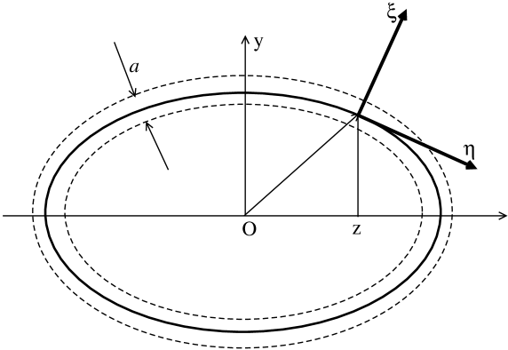
Figure 1: The ES and local $\xi,\eta$ coordinates. The ES in the cylindrical $y,z$ coordinates with the symmetry axis $z$ and diffuseness parameter $a$ are shown schematically by the thick solid and dashed curves (after Ref. magsangzh ).

	SkM∗	SkM	SIII	SGII	RATP	SkP	T6	SkI3	SLyb	SLy4	SLy5	SLy6	SLy7
$\overline{\rho}$ (fm-3)	0.16	0.16	0.15	0.16	0.16	0.16	0.16	0.16	0.16	0.16	0.16	0.17	0.16
$b_{V}$ (MeV)	15.8	15.8	15.9	15.6	16.0	15.9	16.0	16.0	16.0	16.0	16.0	16.0	16.0
$K$ (MeV)	217	217	355	215	240	201	236	258	230	230	230	230	230
$J$ (MeV)	30.1	31.0	28.2	26.9	29.3	30.0	30.0	34.8	32.0	32.0	32.1	31.9	31.9
${\cal C}_{+}$ (MeV$\cdot$fm5)	57.6	52.9	49.4	43.9	60.2	60.1	55.1	51.8	59.5	59.5	59.3	54.0	52.7
${\cal C}_{-}$ (MeV$\cdot$fm5)	-4.79	-4.69	-5.59	-0.94	13.9	-20.2	0	12.6	-22.3	-22.3	-22.8	-15.6	-13.4
$a$ (fm)	0.52	0.50	0.59	0.45	0.55	0.50	0.52	0.53	0.53	0.53	0.53	0.52	0.50
$a_{d}$ (fm)	0.63	0.58	0.73	0.58	0.71	0.71	0.70	0.63	0.68	0.68	0.68	0.61	0.61
$c_{sym}$	3.26	3.21	3.42	6.02	2.00	1.52	$\infty$	2.20	1.59	1.59	1.57	1.80	1.93
$\beta$	-0.64	-0.69	-0.57	-0.54	-0.52	-0.37	-0.45	-0.65	-0.55	-0.55	-0.58	-0.59	-0.65
$b_{S}^{+}$ (MeV) chaban ; reinhard	16.0	16.0	17.0	14.8	17.9	17.9	17.9	16.0	16.7	18.1	18.0	17.4	17.0
$b_{S}^{+}$ (MeV)	21.2	19.9	14.5	18.7	21.7	24.9	21.3	18.3	21.7	21.7	21.5	21.6	19.6

TABLE I. Basic parameters of the Skyrme forces from Refs. chaban ; reinhard and the isoscalar surface energy constants $b_{S}^{(+)}$ of Eq. (12); the critical parameters $a$ [Eq. (3)] and $a_{d}$ [Eq. 5] for the nuclear diffuseness edge, the isoscalar and isovector constants $C_{\pm}$ of the energy density [Eq. (2)], $c_{sym}$ [Eq. (6)] and the spin-orbit constant $\beta$ [see below Eq. (3)]; SLyb denotes shortly SLy230b of Ref. chaban .

	SkM∗	SkM	SIII	SGII	RATP	SkP	T6	SkI3	SLyb	SLy4	SLy5	SLy6	SLy7
$k_{S,0}$ (MeV)	-3.26	-3.84	-2.65	-0.71	5.25	-5.36	0	6.93	-7.51	-7.54	-8.14	-7.45	-6.95
$k_{S}$ (MeV)	-0.77	-1.90	-0.52	-0.21	1.42	-1.93	0	4.88	-4.24	-4.38	-6.96	-6.72	-6.32
$\nu_{0}$	3.08	3.06	3.14	3.64	2.38	2.17	4.32	2.53	2.12	2.12	2.12	2.22	3.32
$\nu$	0.34	0.46	1.42	17.9	0.45	1.76	4.30	0.56	0.44	0.44	0.59	0.65	0.67
$Q_{0}$ (MeV)	7744	9487	6255	16879	-371	3815	$\infty$	-6314	4771	4794	5178	5350	5703
$Q$ (MeV)	398	234	2168	60998	-270	823	$\infty$	-140	105	104	87	98	109
$\tau_{0}/I$	0.021	0.020	0.021	0.0065	0.038	0.037	0	0.033	0.040	0.40	0.040	0.037	0.035
$\tau/I$	0.044	0.090	0.015	0.0019	0.072	0.048	0	0.187	0.20	0.21	0.28	0.26	0.24
$D_{HD}$ (MeV)	85 86	85 86	82	82	90 89	87	88	105 100	81 84	81 84	79 83	81 85	81 84
$D_{FLD}$ (MeV)	73 82	71 76	79 104	74 77	77 87	70 69	86 88	101 106	80 90	80 90	76 84	80 91	77 89

TABLE II. Isovector energy $k_{S}$ and stiffness $Q$ coefficients are shown for several Skyrme forces chaban ; reinhard ; $\nu$ is the constant of Eq. (20); $\tau/I$ is the neutron skin calculated by Eq. (18); quantities $k_{S,0}$, $\nu_{0}$, $Q_{0}$ and $\tau_{0}$ are calculated with $\beta=0$; the intervals of monotonic functions $D_{HD}(A)$ and $D_{FLD}(A)$ for the HD and FLD models in the last two lines are related to $A\approx 50-200$ (the last line is taken from Ref. BMV ).

References

- (1) V. M. Strutinsky and A. S. Tyapin, JETP (Sovjet Phys.) (USSR) 18, 664 (1964).
- (2) V. M. Strutinsky, A. G. Magner, and M. Brack, Z. Phys., A 319, 205 (1984).
- (3) V.M. Strutinsky, A.G. Magner, and V. Yu. Denisov, Z. Phys., A 322, 149 (1985).
- (4) M. Brack, C. Guet, and H.-B. Hakansson, Phys. Rep. 123, 275 (1985).
- (5) A. G. Magner, A. I. Sanzhur, and A. M. Gzhebinsky, Int. J. Mod. Phys. E 18, 885 (2009).
- (6) J. P. Blocki, A. G. Magner, and A. A. Vlasenko, Nucl. Phys. and At. Energy, 13, 333 (2012).
- (7) W.D. Myers, W.J. Swiatecki, Ann. Phys. 55, 395 (1969); 84, 186 (1974).
- (8) W. D. Myers, W. J. Swiatecki, Nucl.Phys. A 336, 267 (1980); 601, 141 (1996).
- (9) W. D. Myers et al., Phys. Rev. C 15, 2032 (1977).
- (10) W. D. Myers, W. J. Swiatecki, and C. S. Wang, Nucl.Phys. A 436, 185 (1985).
- (11) P. Danielewicz, Nucl. Phys. A727, 233 (2003).
- (12) M. Samyn, S. Gorily, M. Bender, and J.M. Pearson, Phys. Rev. C, 70, 044309 (2004).
- (13) P. Danielewicz, J. Lee, Int. J. Mod. Phys. E18, 892 (2009).
- (14) M. Centelles, X. Roca-Maza, X. Vinas, and M. Warda, Phys. Rev. Lett., 102, 122502 (2009).
- (15) M. Warda, X. Vinas, X. Roca-Maza, and M. Centelles, Phys. Rev. C 80, 024316 (2009); 81, 054309 (2010).
- (16) M. Centelles, X. Roca-Maza, X. Vinas, and M. Warda, Phys. Rev. C 82, 054314 (2010).
- (17) X. Roca-Maza, M. Centelles, X. Vinas, and M. Warda, Phys. Rev. Lett. 106, 252501 (2011).
- (18) S. Siem et al., 4th International Conference on Current Problems in Nuclear Physics and Atomic Energies. Book of Abstracts, (Institute for Nuclear Research, National Academy of Sciences of Ukraine, Kyiv, 2012), p. 26.
- (19) A. Repko, R.-G. Reinhard, V. O. Nesterenko, and J. Kvasil, Phys. Rev. C87, 024305 (2013).
- (20) V.Yu. Denisov, Sov. J. Nucl. Phys. 43, 28 (1986).
- (21) V.M. Kolomietz and A.G. Magner, Phys. Atom. Nucl. 63, 1732 (2000).
- (22) V.M. Kolomietz, A.G. Magner, and S. Shlomo, Phys. Rev. C 73, 024312 (2006).
- (23) E. Chabanat et al., Nucl.Phys. A 627, 710 (1997); ibid 635, 231 (1998).
- (24) R.-G. Reinhard and H. Flocard, Nucl. Phys. A 585, 467 (1995).
- (25) M. Bender, P.-H. Heenen, P.-G. Reinhard, Rev. Mod. Phys. 75, 121 (2003).
- (26) J.R. Stone and R.-G. Reinhard, Prog. Part. Nucl. Phys. 58, 587 (2007).
- (27) J. Erler, C. J. Horowitz, W. Nazarevich, M. Rafalski, and P.-G. Reinhard, arXiv:1211.6292v1 [nucl-th] 27 Nov. 2, 2012.
- (28) Aa. Bohr and B. Mottelson, Nuclear structure (W.A. Benjamin, New York, 1975), Vol. II.
- (29) A. G. Magner, V. M. Strutinsky, Z. Phys. A 322, 633 (1985).
- (30) A.G. Magner, Sov. J. Nucl. Phys. 45, 235 (1987).
- (31) J.M. Eisenberg, W. Greiner, Nuclear Theory, Vol. 1, Nuclear Models Collective and Single-Particle Phenomena (North-Holland Publishing Company Amsterdam-London, 1970).
- (32) V. A. Plujko, R. Capote, O. M. Gorbachenko, and V. M. Bondar, in Proceedings of the 3rd International Conference on Current problems in Nuclear Physics and Atomic Energy, Kyiv, Ukraine, June 2010 (Institute for Nuclear Research, National Academy of Sciences of Ukraine, Kyiv, 2011), part 1, pp. 342-346.
- (33) V. A. Plujko, O. M. Gorbachenko, V. M. Bondar, and R. Capote, J. Korean Phys. Soc., 59, 1514 (2011).
- (34) V. A. Plujko, R. Capote, and O. M. Gorbachenko, Atomic Data and Nuclear Data Tables, 97, 567 (2011).
- (35) A. M. Gzhebinsky, A. G. Magner, S. N. Fedotkin, Phys. Rev. C 76, 064315 (2007).
- (36) J. P. Blocki, A. G. Magner and I. S. Yatsyshyn, Int. J. Mod. Phys. E 21, 1250034 (2012).
- (37) J. P. Blocki and A. G. Magner, in IXth International Nuclear Physics Workshop ”Maria & Pierre Curie”, September 2012, Kazimierz Dolny, Poland [Phys. Scr., T 153 (2013) (to be published)].