Renormalized entropy for one dimensional discrete maps: periodic and quasi-periodic route to chaos and their robustness

Abstract

We apply renormalized entropy as a complexity measure to the logistic and sine-circle maps. In the case of logistic map, renormalized entropy decreases (increases) until the accumulation point (after the accumulation point up to the most chaotic state) as a sign of increasing (decreasing) degree of order in all the investigated periodic windows, namely, period-$2$, $3$, and $5$, thereby proving the robustness of this complexity measure. This observed change in the renormalized entropy is adequate, since the bifurcations are exhibited before the accumulation point, after which the band-merging, in opposition to the bifurcations, is exhibited. In addition to the precise detection of the accumulation points in all these windows, it is shown that the renormalized entropy can detect the self-similar windows in the chaotic regime by exhibiting abrupt changes in its values. Regarding the sine-circle map, we observe that the renormalized entropy detects also the quasi-periodic regimes by showing oscillatory behavior particularly in these regimes. Moreover, the oscillatory regime of the renormalized entropy corresponds to a larger interval of the nonlinearity parameter of the sine-circle map as the value of the frequency ratio parameter reaches the critical value, at which the winding ratio attains the golden mean.

I Introduction

With the advent of the science of complexity, numerous complexity measures have been proposed. These measures can be grouped mainly in two categories: first group follows the route of constructing the shortest computer program corresponding to a given string. The well-known Kolmogorov-Chaitin Kolmogorov ; Chaitin and logical depth Bennett measures fall into this category. The second group follows the information-theoretic approaches whose main examples can be given as effective complexity, thermodynamic depth Lloyd , Shiner-Davison-Landsberg Shiner and Lòpez-Ruiz-Mancini-Calbet measures Calbet .

The information-theoretic approaches are founded on the main idea of multiplying a measure of order by that of disorder. In this sense, these approaches rely heavily on the definitions of entropy as a measure of order/disorder. For example, Shiner-Davison-Landsberg Shiner uses Boltmann-Gibbs-Shannon (BGS) entropy of the physical system in its definition, while thermodynamic depth as a complexity measure considers the entropy of the ensemble focusing on the entire history of the system under investigation Lloyd .

However, to the best of our knowledge, none of these complexity measures have been constructed particularly to deal with the non-equilibrium stationary states resulting from the external influence of a field. Such a complexity measure has been recently introduced by Saparin et al. and applied to logistic map Kurths1 , heart rate variability Kurths2 ; Kurths3 and to the analysis of electroencephalograms of epilepsy patients Kurths4 . This new complexity measure is an information-theoretic one and is called renormalized entropy, historically originating from Klimontovich’s S-theorem (The letter S here stands for the self-organization) Klimontovich1 ; Klimontovich2 ; Klimontovich3 ; Klimontovich4 ; Klimontovich5 . The renormalized entropy is theoretically equivalent to negative relative entropy between a reference distribution and any other distribution obtained either analytically or numerically through a time-series analysis Kopitzki ; Grassberger . However, it is not only associated with the relative entropy, since an additional procedure of renormalization is also introduced. The process of renormalization is used in order to compare two states by equating their mean energies so that non-equilibrium stationary states attain the same mean energy, thereby mimicking the ordinary closed system formalism. Combining renormalization and the relative entropy, the renormalized entropy decreases as the control parameter increases, indicating the relative degree of order in the system as first suggested by Haken Haken in the context of self-organization.

On the other hand, another related issue in the context of self-organization is the existence of bifurcations often observed in nonlinear dynamical systems: the systems possessing a stable fixed point become unstable as they recede away from this stable fixed point as a result of increasing nonlinear effects. These systems eventually pave their way to the new stable branches through bifurcations. For the system away from the stable fixed point, this process continues until the system sets in a new stationary state, thereby increasing its order as a signature of self-organization due to the non-linearity, dissipation and the non-equilibrium exhibited by the system (see the detailed discussion by Nicolis and Prigogine in Ref. Prigogini ). Physical processes such as Rayleigh-Benard (Rayleigh1916, ; Rayleigh-Benard1985, ), Taylor instability (Taylor1923, ) experiments, bacterial (Benjacob1994, ) and Dictyostelium discoideum (Palsson1996, ) colonies fall into the aforementioned category. These systems, being open due to exchange of energy and/or matter with its surroundings, can not be analyzed in terms of usual H-theorem, since it is valid only for isolated systems. Therefore, Prigogine proposed a more general form of the second law i.e. $\Delta{S}=\Delta_{i}{S}+\Delta_{e}{S}$ where $\Delta_{i}{S}$ is the entropy produced inside the system and $\Delta_{e}{S}$ is the transfer of entropy across the boundaries of the system. In this more general setting, $\Delta_{i}{S}\geq 0$ whereas $\Delta_{e}{S}$ can be positive or negative depending on the flow of energy across the boundaries of the system. The overall sign of $\Delta{S}$ is determined by the interplay between $\Delta_{i}{S}$ and $\Delta_{e}{S}$. All the aforementioned models of self-organization requires $\Delta{S}<0$ until the system sets in the stationary state corresponding to the most ordered pattern.

The paper is organized as follows. In Section 2, calculation methods of the renormalized entropy is given. In section 3, this complexity measure is applied to discrete maps possessing different universality classes i.e. to the logistic map which has periodic route to chaos and its self similar windows like period 3 and period 5 to show its robustness and to sine-circle map which has periodic and quasi-periodic route to chaos. Finally, we discuss our results and compare the two different routes to chaos in terms of the renormalized entropy.

II Method

II.1 An overview for the renormalized entropy

Let us consider a generic dynamical map $X_{t+1}=G(X_{t},a)$ where $t$ and $a$ denote the number of iterations and the corresponding control parameter of the dynamical map, respectively. A small change in the value of the control parameter, $\Delta{a}$, yields two normalized distributions i.e. $f(X,a)=f_{0}(X)$ and $f(X,(a+\Delta{a}))=f_{1}(X)$. The corresponding Shannon entropies read

$$S\left({f_{0}(X)}\right)=-\int f_{0}(X)\,\ln f_{0}(X)dX\,\,\,\,,\,\,\,\,S\left({f_{1}(X)}\right)=-\int f_{1}(X)\,\ln f_{1}(X)dX\,.$$ (1)

Let us now assume that the system i.e. dynamical map under scrutiny evolves in such a manner that the state with index $1$ is evolved to through increasing order, namely, the system becomes self-organized as the control parameter increases. Then, setting equilibrium temperature $T_{eq}=1$, the normalized Boltzmann-Gibbs distribution reads

$$f_{0}(X)=\exp\left[-H_{eff}(X)\right]$$ (2)

with the following effective energy

$$H_{eff}=-\ln f_{0}(X).$$ (3)

S-theorem by Klimontovich equates the effective energies of the concomitant states i.e. renormalizes the states in order to apply H-theorem of Boltzmann to open systems, implying $\Delta_{e}{S}=0$ in the second law formulation of Prigogine (Nobel, ) and $f_{0}(X)\rightarrow\tilde{f}_{0}(X)$ to compensate for the mean energy difference i.e. turning open system into a closed one. Denoting the renormalized state by $tilde$, one can write

$$\tilde{f}_{0}(X)=C\,\left[f_{0}(X)\right]^{\beta_{eff}}=C\,\exp\left[\frac{-H_{eff}(X)}{T_{eff}}\right]$$ (4)

where $C$ is the normalization constant. To check whether any heat intake occurs during self-organization, to form spatially more ordered patterns, through dissipation as a result of interaction with the environment, $T_{eff}$ is calculated from the equality of mean energies

$$\int\tilde{f}_{0}(X)\,\ln f_{0}(X)dX=\int f_{1}(X)\,\ln f_{0}(X)dX\,.$$ (5)

If heat intake is needed for the process of self-organization such as Rayleigh-Benard convection resulting in spatially ordered hexagonal patterns at the stationary state (Rayleigh1916, ; Rayleigh-Benard1985, ), then one expects, comparing the equilibrium and non-equilibrium states, $T_{eff}>1$, since $T_{eq}=1$. Otherwise, we deduce that our assumption regarding the more disorderliness of the initial distribution is not correct, indicating the second distribution to be more disordered. Therefore, when this is the case, one renormalizes the second distribution. The measure of relative degree of order for these compared states can then be given as the difference of entropies

$$\Delta\tilde{S}=S\left({f_{1}(X)}\right)-S\left({\tilde{f}_{0}(X)}\right)$$ (6)

which is called renormalized entropy (Anishchenko1994, ).

II.2 Calculation of the spectrum

We use the spectral intensities $P_{0}(w)$ and $P_{1}(w)$ averaged over $M$ periodograms based on the multiplication of the Fourier and the inverse Fourier transformation of the time series of $X_{t}$ in the frequency domain $w$, instead of the density distributions $f_{0}(x)$ and $f_{1}(x)$ in Eqs. [1-6], respectively so that

$$P(w)=\frac{1}{\ell\,\Delta{t}}\left|\Delta{t}\,\sum_{n=0}^{\ell-1}x_{n}\,\exp(-i2{\pi}wn\Delta{t})\right|^{2}\;,$$ (7)

where the sequence $X_{n}$ is a sufficiently long series of values that can be obtained by iterating a mapping by sampling equidistant points and $\ell$ is the length of the samples in every periodogram wessel1 , satisfying $P(w)>0$ and $\sum{P(w)=1}$. Such a Fourier spectra eliminate the ’zeros’ in the distributions and detect different regimes of a deterministic dynamical system.

III Application of the renormalized entropy

To start with, let us consider a $d$-dimensional mapping of the form

$$X_{t+1}=G(X_{t})\;$$ (8)

on some $d$-dimensional phase space $X$. We can numerically generate data from such a mapping equation that describes dynamics of a specific dynamical system. We particularly focus on two examples. One is the logistic map given as

$$X_{t+1}=4\,a\,X_{t}\,(1-X_{t})$$ (9)

where $a\in[0,4]$ is a control parameter and the map is confined to the interval $X\in[0,1]$, which exhibits periodic route to chaos. For $a=4$, the system is (semi)conjugated to a Bernoulli shift and strongly mixing. The other is the sine-circle map given as

$$\theta_{t+1}=\theta_{t}+\Omega-\frac{K}{2\pi}\sin{(2\pi\theta_{t})}~{}~{}~{}\mod(1)\;\;$$ (10)

where $0\leq\theta_{t}<1$ is a point on a circle and parameter $K$ (with $K>0$) is a measure of the strength of the nonlinearity, whichs exhibit periodic route to chaos. It describes dynamical systems possessing a natural frequency $\omega_{1}$ which are driven by an external force of frequency $\omega_{2}$ ($\Omega=\omega_{1}/\omega_{2}$ is the bare winding number or frequency-ratio parameter) and belongs to the same universality class of the forced Rayleigh-Benard convection jensen . Winding number for this map is defined to be the limit of the ratio

$$W=\lim_{t\rightarrow\infty}\frac{(\theta_{t}-\theta_{0})}{t}\;\;,$$ (11)

where $(\theta_{t}-\theta_{0})$ is the angular distance travelled after $t$ iterations of the map function. To increase the degree of irrationality of the system, one could use frequency ratio parameter $\Omega$ corresponding to winding number $W$ that approaches the golden mean gradually by following the sequence of ratios of the Fibonacci numbers (${F_{n}}/{F_{n+1}}$). The map is monotonic and invertible (non-monotonic and non-invertible) for $K<1$ ($K>1$) and develops a cubic inflexion point at $\theta=0$ for $K=1$.

Considering technical details, it is important to emphasize that we added Gaussian white noise into systems in Eqs. (9) and (10) with a small intensity $(D_{B}=10^{-14})$, which is called basic noise, to every state. The low intensity of the noise is chosen so as not to influence the dynamics of these systems. This procedure enables a continuous spectral distribution $P(w)$. After 65536 transients, we generated the discrete sequences with the length of $4096\times 18$ points separately obtained from Eq. (9) and (10). Finally, the spectrum of 18 shifted windows of 4096 samples $(\Delta{t}=0.5~{}s)$ is estimated and averaged.

III.1 Renormalized entropy and its robustness at different windows for the logistic map: periodic route to chaos

One of the dynamical systems possessing bifurcation properties can be cited as the logistic map, which moves from a unique stable fixed point to the critical accumulation point possessing infinite periods through the periodic doubling route. Having reached the critical accumulation point, the system enters into the chaotic regime and from this point on it moves under the influence of chaotic band merging (i.e., inverse period-doubling). It should also be remarked that periodic windows with different periods but albeit self-similar structures are also found in this chaotic regime.

We now present the results concerning the behavior of the renormalized entropy and the bifurcation properties in the regions of period $2$, $3$ and $5$. Before proceeding further, we note that the renormalized entropy has already been applied to the logistic map for period-2 window by Saparin et al. in Ref. Kurths1 . Our aim in this section is to investigate all other self-similar windows to check whether the renormalized entropy behaves consistently as a complexity measure, i.e., to check its robustness. Fig. 1a in particular shows the behavior of the renormalized entropy in the period 2 region where control parameter $a$ lies between $3$ and $4$. In this region, relative degree of order increases until the period accumulation point i.e., $a_{c}^{\left(2\right)}\sim 3.569$ as the system evolves from the equilibrium state to a new stationary state in accordance with the self-organization process. As a signature of the detection of the self-organization in this region then, the relative entropy monotonically decreases as expected. After the period $2$ accumulation point onward until the most chaotic state with $a=4$, the relative degree of order decreases, since band-merging (as opposed to bifurcation in the previous region) is exhibited by the system in this region. Therefore, the renormalized entropy increases in the aforementioned region in a non-monotonic manner. To sum up, for an open non-equilibrium dynamical system which approaches the stationary state through period-doubling and recedes away from the stationary state by means of band-merging, the behavior of the renormalized entropy conforms to the dictum of Prigogine i.e., order out of chaos. In Fig. 1b, we zoom in the period $3$ window i.e., the largest self-similar window in the period $2$ region. The control parameter values for this window are confined in the interval between $3.832$ and $3.856$. Similarly to the period $2$ window, the relative degree of order monotonically increases up to the period accumulation point $a_{c}^{\left(3\right)}\sim 3.849$, and thereafter decreases non-monotonically. Accordingly, the relative entropy decreases up to the accumulation point, and begins to increase after the period accumulation point. It is worth noting the sudden, unexpected changes in the values of the renormalized entropy which signal the existence of the self-similar windows in the chaotic region. Fig. 1c shows the behavior of the renormalized entropy in the period $5$ window, which is one of the self-similar windows in the logistic map. Due to the self-similarity, a behavior similar to the one in period $3$ is exhibited by the renormalized entropy: it decreases almost up to $a_{c}^{\left(5\right)}\sim 3.743$, and then begins to increase in accordance with the decrease in the relative degree of order. Finally, it is interesting to observe the turns in the relative degree of order for each of the three period accumulation points representing the stationary state of a non-equilibrium dynamical system possessing inherent fractal structure.

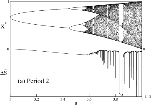
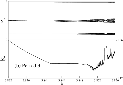
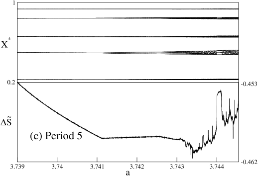
Figure 1: The bifurcation diagram (upper panels) and renormalized entropy (lower panels) for period $2$ (a), period $3$ (b) and period $5$ (c) of the logistic map.

III.2 Renormalized entropy for the sine-circle map: quasi-periodic route to chaos

The sine-circle map can exhibit periodic, quasi-periodic or chaotic behaviors depending on the frequency ratio and the nonlinearity parameters i.e., $\Omega$ and $K$, respectively. For $0\leq K\leq 1$, the system dynamics is either periodic (frequency-locked) or quasi-periodic depending on the value of the frequency ratio parameter $\Omega$ being rational or irrational. As the nonlinearity parameter $K$ approaches zero, the system exhibits quasi-periodic behavior for all values of the frequency ratio parameter $\Omega$.

As the nonlinearity parameter $K$ approaches one, frequency-locked steps extend and occupy all $\Omega$ axes where $K$ is equal to one. In this case, there is a special fraction of $\Omega$ value called the most irrational $\Omega_{c}$, corresponding to the “golden mean” winding number $W$ if frequency ratio parameter $\Omega$ is locked to its critical value $\Omega_{c}$. Shortly after this critical value on $(K,\Omega)$ plane, $(1,\Omega_{c})$ is the edge of quasi-periodic route to chaos since chaotic behavior can occur. All these characteristic shapes on $(K,\Omega)$ plane is called “Arnold Tongues” in the literature. For the $K>1$ region where the nonlinearity parameter $K$ is dominant on the system dynamics, there could be periodic regions with different periods, chaotic regions, and so edges of periodic route to chaos. Also, for this region, there could be periodic windows possessing same universality class with the logistic map.

Fig. 2 shows the behavior of the renormalized entropy and the bifurcations of the sine-circle map for $\Omega_{4}=0.592523777531...$, $\Omega_{5}=0.611736528912...$ and $\Omega_{c}=0.606661063469...$ obtained from Eqs. (10-11), respectively where the nonlinearity parameter $K$ lies between zero and $2.5$. The reference state for the renormalized entropy is chosen to be the one with $K=0$ and $\Omega=0$ where the system evolves towards a unique stable point. Note that the degree of irrationality of the system increases as one moves from Fig. 2a towards Fig. 2c.

In each of the aforementioned figures, the oscillatory behavior of the renormalized entropy is observed when the system is in the quasi-periodic regime. This oscillatory behavior is exhibited when $K\in\left[0,0.80\right]$, $\left[0,0.95\right]$, $\left[0,1\right]$ for the cases $\Omega$=$\Omega_{4}$, $\Omega_{5}$ and $\Omega_{c}$, respectively. It is interesting to note that the interval of the nonlinearity parameter $K$ increases in regard to the oscillatory behavior of the renormalized entropy as the value of the frequency ratio parameter reaches the critical value $\Omega_{c}$, at which the winding ratio $W$ attains the golden mean. As a result, the renormalized entropy can detect the quasi-periodic regime as can be seen from Fig. 2. It is worth noting that the Lyapunov exponent is zero for all quasi-periodic regions as well as periodic regimes at the bifurcation points hilborn . In this sense, the renormalized entropy is superior to the Lyapunov exponent, since the renormalized entropy behaves in a distinct manner in both of the aforementioned regions. Many chaotic and periodic regions with different periods are present in Fig. 2 for the nonlinearity parameter $K$ values $K\in\left[0.80,2.50\right]$, $\left[0.95,250\right]$, $\left[1,2.5\right]$ corresponding to $\Omega$=$\Omega_{4}$, $\Omega_{5}$ and $\Omega_{c}$, respectively. The renormalized entropy always attains values close to zero in these intervals for the chaotic regions, while it decreases with the increasing number of periods in the periodic regions until it reaches the edge of chaos. This can be considered as the signature of the relative degree of order within the system.

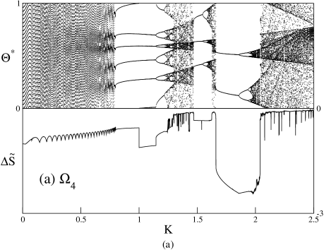
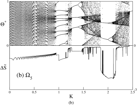
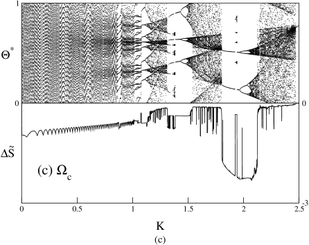
Figure 2: The bifurcation diagram (upper panels) and renormalized entropy (lower panels) for $\Omega_{4}$ (a), $\Omega_{5}$ (b) and $\Omega_{c}$ (c) of the sine-circle map.

It is well-known that the sine-circle map is in the same universality class as the logistic map for $K\in\left[3.19,3.81\right]$ when $\Omega=\Omega_{c}$. Fig. 3 shows the bifurcation and the renormalized entropy for this particular window. The renormalized entropy behaves exactly as it does in Fig. 1a for the logistic map, thereby indicating that different dynamical maps exhibit same behavior in the regions falling into the same universality class.

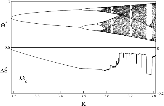
Figure 3: The bifurcation diagram (upper panel) and renormalized entropy (lower panel) of the region possessing the same universality class with the logistic map for $\Omega_{c}$ of the the sine-circle map.

IV Conclusions

Despite the presence of many different complexity measures, the ones enabling a local comparison of the distributions are quite few (for a recent example, see Ref. romera ). One such measure of relative nature is the renormalized entropy introduced by Klimontovich, Kurths and coworkers Kurths1 ; Kurths2 ; Kurths3 ; Kurths4 ; Klimontovich1 ; Klimontovich2 ; Klimontovich3 ; Klimontovich4 ; Klimontovich5 ; Kopitzki . In this work, the renormalized entropy is used to analyze the logistic and sine-circle maps. In the former example of the logistic map, renormalized entropy decreases (increases) up to the accumulation point (after the accumulation point until the most chaotic state) as a sign of increasing (decreasing) relative degree of order in all the self-similar periodic windows, thereby proving the robustness of this complexity measure. By robustness, we emphasize the similarity of the behavior of the renormalized entropy in all the self-similar windows, therefore removing the doubt concerning a possible accidental feature of the renormalized entropy as a complexity measure. On the other hand, The aforementioned observed changes in the renormalized entropy are reasonable, since the bifurcations occur before the accumulation point, after which the band-merging, in opposition to the bifurcations, is exhibited. On top of the precise detection of the accumulation points in all these windows, we see that the renormalized entropy can detect the self-similar windows in the chaotic regime by exhibiting sudden changes in its values. For the sine-circle map, on the other hand, the renormalized entropy detects also the quasi-periodic regimes by signaling oscillatory behavior particularly in these regimes. Moreover, the oscillatory regime of the renormalized entropy corresponds to a larger interval of the nonlinearity parameter of the sine-circle map as the value of the frequency ratio parameter reaches the critical value, at which the winding ratio attains the golden mean. Lastly, we remark that the renormalized entropy is superior to the Lyapunov exponent as a complexity measure, since the renormalized entropy can detect the quasi-periodic regimes as well as the periodic regimes at the bifurcation points in a distinct manner whereas the Lyapunov exponent is zero for both of these regions, hence detecting no difference at all hilborn .

V Acknowlegments

This work has been supported by TUBITAK (Turkish Agency) under the Research Project number 112T083. U.T. is a member of the Science Academy, Istanbul, Turkey.

References

- (1) A. N. Kolmogorov, Probl. Inf. Transm. 1 (1965) 1.
- (2) G. Chaitin, J. Assoc. Comput. Mach. 13 (1966) 145.
- (3) C. H. Bennett, Found. Phys. 16 (1986) 585.
- (4) H. Pagels and S. Lloyd, Ann. Phys. 188 (1988) 186.
- (5) J. S. Shiner, M. Davison, and P. T. Landsberg, Phys. Rev. E 59 (1999) 1459.
- (6) R. Lòpez-Ruiz, H.L. Mancini, and X. Calbet, Phys. Lett. A 209 (1995) 321.
- (7) P. Saparin, A. Witt, J. Kurths, and V. Anischenko, Chaos, Solitons and Fractals 4 (1994) 1907.
- (8) J. Kurths et al., Chaos 5 (1995) 88.
- (9) A. Voss et al., Cardiovasc. Res. 31 (1996) 419.
- (10) K. Kopitzki, P. C. Warnke, and J. Timmer, Phys. Rev. E 58 (1998) 4859.
- (11) Yu. L. Klimontovich, Physica A 142 (1987) 390.
- (12) Yu. L. Klimontovich, Chaos, Solitons and Fractals 5 (1994) 1985.
- (13) Yu. L. Klimontovich, Turbulent Motion and the Structure of Chaos: A New Approach to the Statistical Theory of Open System, Dordrecht: Kluwer Academic Publishers (1991).
- (14) Yu. L. Klimontovich, Z. Phys. B 66 (1987) 125 .
- (15) Yu. L. Klimontovich and M. Bonitz, Z. Phys. B 70 (1988) 241.
- (16) K. Kopitzki, P. C. Warnke, and J. Timmer, Phys. Rev. E 58 (1998) 4859.
- (17) R. Q. Quiroga, J. Arnold, K. Lehnertz, and P. Grassberger, Phys. Rev. E 62 (2000) 8380.
- (18) H. Haken, Information and Self-organization: A Macroscopic Approach to Complex Systems. Berlin: Springer Verlag (2000).
- (19) G.Nicolis and Prigogini, Self-Organization in Nonequilibrium Systems (Wiley-Interscience, New York, 1977), See especially Chapter VII.
- (20) N. Wessel, A. Voss, J. Kurths, P. Saparin, A. Witt, H. J. Kleiner and R. Dietz, Comput. Cardiol., pp.137-140 (1994).
- (21) M.H. Jensen, L.P. Kadanoff, A. Libchaber, I. Procaccia and J. Stavans, Phys. Rev. Lett. 55, 2798 (1985).
- (22) E. Ott, Chaos in Dynamical Systems (Cambridge University Press, Cambridge, 2002), p. 219.
- (23) R.C. Hilborn, Chaos and Nonlinear Dynamics (Oxford University Press, New York, 1994), p. 390.
- (24) E. Romera, K. D. Sen, and Á. Nagy, J. Stat. Mech. (2011) P09016.
- (25) P. Saparin, A. Witt, J. Kurths and V. Anishchenko, Chaos, Solitons and Fractals, 4, 1907 (1994).
- (26) I. Prigogine, Time, Structure and Fluctuations, Nobel Lecture (1997).
- (27) L. Rayleigh, Philos. Mag., 32, 529 (1916).
- (28) , Phys. Rev. Lett., 55, 2798 (1985).
- (29) G. I. Taylor, Philos. Trans. Roy. Soc. London Ser. A, 223, 289 (1923).
- (30) E. Benjacob, O. Schochet, A. Tenenbaum, I. Cohen, A. Czirok, T. Vicsek, Nature, 368, 46 (1994).
- (31) E. Palsson, E. C. Cox, Proc. Natl. Acad. Sci., 93, 1151 (1996).