Width of photon decay in magnetic field:
elementary semiclassical derivation and sensitivity to Lorentz violation

Abstract

We present an elementary derivation of the width of photon decay in a weak magnetic field using the semiclassical method of worldline instantons. The calculation is generalized to a model of quantum electrodynamics with broken Lorentz symmetry. Implications for the search of deviations from Lorentz invariance in the cosmic ray experiments are discussed.

1 Introduction

   Semiclassical methods are widely used in modern quantum field theory. They provide a powerful tool to investigate non-perturbative phenomena. The well-known example is the false vacuum decay [1, 2]. Equations of motion have a solution, called bounce, that interpolate between false and true vacua. The probability of decay is proportional to the exponent (with the minus sign) of the Euclidean action evaluated on the bounce.

The similar calculation arises in another class of processes, particle production in external backgrounds. The simplest example is the Schwinger effect — spontaneous creation of electron-positron pairs in external electric field. The probability of pair production is expressed through the thermal partition function of a certain quantum mechanical problem [3]. This partition function is evaluated in the saddle point approximation; the solutions of the saddle point equations, called ’worldline instantons’, are interpreted as trajectories of a particle in an auxiliary periodic time. Semiclassical treatment of Schwinger-like processes has been generalized to the cases of time-dependent and inhomogeneous electromagnetic field [4] and to the photon-stimulated Schwinger pair creation in application to the laser physics [5]. In this article we study the similar process — the photon decay into an electron-positron pair in magnetic field. We will be interested in the weak-field limit where the semiclassical method is applicable. For a review of methods used in the opposite case of the strong magnetic field see [6].

The probability of the photon decay in magnetic field was calculated long time ago independently by [7, 8]. The corresponding matrix element has been computed in the semiclassical approximation in terms of the overlap of electron wavefunctions (eigenfunctions of the Dirac equation in the uniform magnetic field) in the coordinate representation. In the weak-field limit the photon decay is exponentially suppressed,

$$\Gamma\propto\exp\left(-\frac{8m^{3}}{3\omega eH\sin\varphi}\right).$$ (1)

Here $\omega$ is the energy of the photon, $H$ is the value of the uniform magnetic field, $\varphi$ denotes the angle between the photon momentum and the magnetic field, $e$ and $m$ are the electron charge and mass; it is assumed that the photon energy is much higher than the electron mass, $\omega\sin\varphi\gg m$ (but still $\omega eH\sin\varphi\ll m^{3}$). The calculation of [7, 8] is technically quite involved. The approach based on the ’worldline instantons’ adopted in the present paper is significantly simpler and has a clear geometrical interpretation. To the best of our knowledge, it has not been applied to the process of pair production in magnetic field so far.

Due to its simplicity, our method can be easily generalized to models beyond the standard QED. This is illustrated in the second part of the paper where we study the process of gamma decay in magnetic field in a model of electrodynamics without Lorentz invariance (LI). It is possible that deviation from LI can appear at very high energies, unaccessible to present-day accelerators. This scenario is suggested by several approaches to the theory of quantum gravity [9, 10, 11, 12, 13] and the energy scale where deviations from LI become significant is naturally assumed to lie at the Plank mass $M_{p}$ or a few orders below.

Remarkably, this type of Lorentz violation (LV) can be constrained by cosmic ray observations, see [14] for recent review. Indeed, energies attained by particles of ultra-high energy cosmic rays (UHECR) greatly exceed those achieved in laboratory. Reaching the Earth, cosmic ray primaries interact in the atmosphere and create showers of descendant particles, that can be detected experimentally. The characteristics of the shower depend on the type and energy of the primary.

The process of photon decay in magnetic field plays an important role in these consideration. When an UHECR photon (with energy above $10^{19.5}\,\mbox{eV}$) reaches the magnetic field of the Earth, it decays into an electron and positron. The latter, in turn, produce photons by the synchrotron radiation, giving rise to an electromagnetic cascade. In this way the magnetosphere shower called preshower [15, 16] is created at the altitude of several hundred kilometers above the Earth surface. Preshower accelerates the subsequent shower development in the atmosphere and provides a unique signature for photon-induced showers: pair production probability depends on the perpendicular component of the magnetic field and hence on the arrival direction of the photon. We will find that possible LV significantly affects the probability of the preshower formation. Thus, experimental detection of a preshower would provide a sensitive probe of LV.

The paper is organized as follows. In Sec. 2 we derive Eq. (1) by the semiclassical method of worldline instantons. In Sec. 3 we calculate the width of photon decay in magnetic field in QED with LV. Sec. 4 is devoted to discussion.

2 Photon decay in a weak magnetic field in standard QED

Consider a photon with four-momentum $k_{\mu}=(\omega,{\bf k})$ propagating in the uniform magnetic field ${\bf H}$ at an angle $\varphi$ to its direction. We choose the coordinate system where the magnetic field points along the $x$-axis, ${\bf H}=(H,0,0)$, and the spatial photon momentum lies in the $(x,y)$-plane, ${\bf k}=(\omega\cos\varphi,\omega\sin\varphi,0)$. The photon decay into an $e^{+}e^{-}$ pair is kinematically allowed if $\omega\sin\varphi>2m$. We will assume the photon energy to be well above this threshold, $\omega\sin\varphi\gg m$.

To find the rate of the photon decay we adopt the method similar to that used in [3, 4, 5] for the semiclassical analysis of the Schwinger process. It was shown in these works that in the leading approximation the answer is insensitive to the spin of the electron. As in the present paper we are interested only in the leading order result, we choose to work for simplicity with the scalar QED, described by the Lagrangian

$$\mathcal{L}=-\frac{1}{4}F_{\mu\nu}F^{\mu\nu}+D_{\mu}\phi^{*}D^{\mu}\phi-m^{2}\phi^{*}\phi,$$ (2)

where the covariant derivative $D_{\mu}$ is defined in the usual way, $D_{\mu}\phi=\left(\partial_{\mu}-ieA_{\mu}\right)\phi$.

It follows from the optical theorem that the rate of photon decay is proportional to the imaginary part of the polarization operator

$$\Gamma=\frac{1}{2\omega}\epsilon_{\mu}(k)\epsilon_{\nu}(k)\mbox{Im}\Pi_{\mu\nu}(k),$$ (3)

where $\epsilon_{\mu}(k)$ is the photon polarization vector which we choose to be real. As usual, $\Pi_{\mu\nu}$ is given by the Fourier transform of the correlator of two electromagnetic currents $j_{\mu}=-ie(\phi^{*}D_{\mu}\phi-\phi D_{\mu}\phi^{*})$,

$$\Pi_{\mu\nu}(k)=\int d^{4}y\,{\rm e}^{iky}\langle j_{\mu}(y/2)j_{\nu}(-y/2)\rangle\;.$$ (4)

In the leading order one can neglect the contribution of virtual photons into this correlator which is then expressed in terms of the partition function of the charged scalar in external electromagnetic field,

$$\langle j_{\mu}(y/2)j_{\nu}(-y/2)\rangle=\frac{1}{Z[A_{\mu}]}\frac{\delta}{i\delta A_{\mu}(y/2)}\frac{\delta}{i\delta A_{\nu}(-y/2)}Z[A_{\mu}]\;,$$ (5)

where

$$Z[A_{\mu}]=\int D\phi^{*}D\phi\,{\rm e}^{-\int d^{4}x\left(\left|D_{\mu}\phi\right|^{2}+m^{2}\left|\phi\right|^{2}\right)}=\det\left(-D_{\mu}^{2}+m^{2}\right)=\exp{\rm Tr}\mathop{\rm ln}\nolimits\left(-D_{\mu}^{2}+m^{2}\right)\;.$$ (6)

Note that in defining the partition function we have performed the Wick rotation to the Euclidean signature.

At the next step we use the formula:

$$-\mathop{\rm ln}\nolimits M=\int_{0}^{\infty}\frac{dT}{T}\left({\rm e}^{-MT}-{\rm e}^{-T}\right)\;.$$

This leads to the expression for the partition function in terms of the integral over the “proper time” $T$.

$$Z[A_{\mu}]=Z_{0}\exp\left[-\int_{0}^{\infty}\frac{dT}{T}{\rm e}^{-m^{2}T}{\rm Tr}\left({\rm e}^{TD_{\mu}^{2}}\right)\right].$$ (7)

The operator $\left(-D_{\mu}^{2}\right)$ can be interpreted as the quantum-mechanical Hamiltonian of a point particle in four-dimensional space. Thus, ${\rm Tr}\left({\rm e}^{-T\left(-D_{\mu}^{2}\right)}\right)$ can be considered as its thermal partition function with the proper time $T$ playing the role of the inverse temperature. It is more convenient to work in the Lagrangian formalism, so we make the Legendre transformation and consider the functional integral representation:

$${\rm Tr}\left({\rm e}^{TD_{\mu}^{2}}\right)=\int\limits_{p.b.c.}Dx_{\mu}{\rm e}^{-\int_{0}^{T}d\tau\left(\frac{\dot{x}^{2}_{\mu}}{4}+ie\dot{x}_{\mu}A_{\mu}\right)}.$$

Here we have introduced an auxiliary time $\tau$ and the notation $p.b.c.$ means periodical boundary conditions $x_{\mu}(0)=x_{\mu}(T)$. The partition function becomes

$$Z[A_{\mu}]=Z_{0}\exp\left[-\int_{0}^{\infty}\frac{dT}{T}{\rm e}^{-m^{2}T}\int_{p.b.c}Dx_{\mu}\,{\rm e}^{-\int_{0}^{T}d\tau\left(\frac{\dot{x}^{2}_{\mu}}{4}+ie\dot{x}_{\mu}A_{\mu}\right)}\right].$$ (8)

We now return to the polarization operator (4). Each variational derivative of the partition function with respect to $A_{\mu}$ produces an insertion of the combination $\oint d\tau\dot{x}_{\mu}(\tau)\delta(x(\tau)-y)$ in the functional integral. Also we rescale the auxiliary time $\tau$ to make it vary from $0$ to $1$. This gives,

$$\langle j_{\mu}(y/2)j_{\nu}(-y/2)\rangle\propto \int_{0}^{\infty}\frac{dT}{T}\int_{p.b.c.}Dx_{\mu}\oint d\tau_{1}\oint d\tau_{2}\dot{x}_{\mu}(\tau_{1})\dot{x}_{\nu}(\tau_{2})$$

$$\times\delta(x(\tau_{1})-y/2)\delta(x(\tau_{2})+y/2)\;{\rm e}^{-m^{2}T-\int_{0}^{1}d\tau\left(\frac{\dot{x}^{2}_{\mu}}{4T}+ie\dot{x}_{\mu}A_{\mu}\right)}.$$

The width of the photon decay is given by the imaginary part of the polarization operator in the momentum representation $\mathrm{Im}\,\Pi_{\mu\nu}(k)=\mathrm{Im}\int d^{4}y\,e^{iky}\Pi_{\mu\nu}(y)$. Taking the Fourier transform for the imaginary part of the polarization operator, one obtains

$$\mathrm{Im}\,\Pi_{\mu\nu}(k)\propto\mathrm{Im}\,\int_{0}^{\infty}\frac{dT}{T}\int_{p.b.c.}Dx_{\mu}\oint d\tau_{1}\oint d\tau_{2}\,\dot{x}_{\mu}(\tau_{1})\dot{x}_{\nu}(\tau_{2}){\rm e}^{-S_{m}[x_{\mu};\tau_{1},\tau_{2}]},$$ (9)

where

$$S_{m}[x_{\mu};\tau_{1},\tau_{2}]=m^{2}T+\int_{0}^{1}d\tau\left(\frac{\dot{x}_{\mu}^{2}}{4T}+ieA_{\mu}\dot{x}_{\mu}\right)-ik_{\mu}\left(x_{\mu}(\tau_{1})-x_{\mu}(\tau_{2})\right).$$ (10)

This expression has the form of the Euclidean action of a relativistic particle in the external electromagnetic field with two sources of opposite signs located at the proper times $\tau_{1}$ and $\tau_{2}$. The strength of these sources is determined by the photon momentum. Integrating out the parameter $T$ one can obtain the standard form of the relativistic particle action.

We will evaluate the r.h.s. of (9) in the saddle-point approximation. To this end, firstly we find the saddle equations for $T$ and $x_{\mu}(\tau)$. Their solution gives the saddle-point classical trajectory $x_{\mu}^{cl}(\tau)$. At the second step the trajectory is substituted into the action (10). Let us fix the gauge $A_{\mu}=-\frac{1}{2}F_{\mu\nu}x_{\nu}$. Varying over $x_{\mu}$, we obtain (separately for the time and space components of $x_{\mu}$),

$$\frac{\ddot{x}_{0}}{2T}=\omega\left(\delta\left(\tau-\tau_{1}\right)-\delta\left(\tau-\tau_{2}\right)\right),$$ (11)

$$\frac{\ddot{x}_{i}}{2T}-ieF_{ij}\dot{x}_{j}=-i\omega\left[\delta_{i1}\cos\varphi+\delta_{i2}\sin\varphi\right]\left(\delta\left(\tau-\tau_{1}\right)-\delta\left(\tau-\tau_{2}\right)\right).$$ (12)

The variation over $T$ yields,

$$m^{2}-\frac{\int_{0}^{1}d\tau\dot{x}_{\mu}^{2}}{4T^{2}}=0.$$ (13)

We are looking for a solution of Eqs. (11)–(13) that describes a closed trajectory in 4-dimensional spacetime. Solutions of this type are called “worldline instantons”. Note that in general they can be complex (cf. [5]). The solution exists if $|\tau_{1}-\tau_{2}|=\frac{1}{2}$. Without loss of generality we set $\tau_{1}=0,\ \tau_{2}=\frac{1}{2}$. Our solution is composed of two hyperbolic arcs (see Fig. 1) defined on the segments $\tau\in(0,\frac{1}{2})$ and $\tau\in(\frac{1}{2},1)$ respectively,

$$\text{for\leavevmode\nobreak\ \leavevmode\nobreak\ }0<\tau<\frac{1}{2}: \qquad x_{0}^{cl}=\omega T\left(\tau-\frac{1}{2}\right), x_{1}^{cl}=-iA\eta\cos\varphi\,\mathrm{ch}\frac{\eta}{4}\cdot\left(\tau-\frac{1}{4}\right),$$ (14)

$$x_{2}^{cl}=-iA \sin\varphi\,\mathrm{sh}\left(\eta\left(\tau-\frac{1}{4}\right)\right), x_{3}^{cl}=-A\sin\varphi\,\left[\mathrm{ch}\left(\eta\left(\tau-\frac{1}{4}\right)\right)-\mathrm{ch}\frac{\eta}{4}\right];$$

$$\text{for\leavevmode\nobreak\ \leavevmode\nobreak\ }\frac{1}{2}<\tau<1: \leavevmode\nobreak\ \leavevmode\nobreak\ \leavevmode\nobreak\ \leavevmode\nobreak\ \leavevmode\nobreak\ x_{0}^{cl}=-\omega T\left(\tau-\frac{1}{2}\right), x_{1}^{cl}=iA\eta\cos\varphi\,\mathrm{ch}\frac{\eta}{4}\cdot\left(\tau-\frac{3}{4}\right),$$ (15)

$$x_{2}^{cl}=iA \sin\varphi\,\mathrm{sh}\left(\eta\left(\tau-\frac{3}{4}\right)\right), x_{3}^{cl}=A\sin\varphi\,\left[\mathrm{ch}\left(\eta\left(\tau-\frac{3}{4}\right)\right)-\mathrm{ch}\frac{\eta}{4}\right].$$

Here parameters $A,\,\eta$ are determined from Eqs. (11), (12):

$$A=\frac{\omega}{2eH\mathrm{ch}\frac{\eta}{4}},\qquad\eta=2TeH.$$ (16)

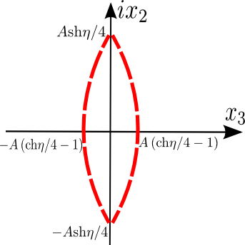
Figure 1: ’Worldline instanton’ — the classical trajectory describing pair production in the magnetic field for the case when the photon momentum is perpendicular to the field direction, $\varphi=\pi/2$. The projection of the trajectory on the plane ($ix_{2},\,x_{3}$) is shown.

Substituting the solution (14)–(16) into (13) one obtains:

$$T=\frac{4m}{\omega eH\sin\varphi}.$$ (17)

The next step is to evaluate the action (10) on the solution. After a straightforward calculations we obtain:

$$S[x_{\mu}^{cl}]=\frac{8}{3}\frac{m^{3}}{\omega eH\sin\varphi}.$$ (18)

The semiclassical method is valid as long as the classical action is large, $S[x_{\mu}^{cl}]\gg 1$. Combining everything together, we obtain the photon decay width:

$$\Gamma=\frac{1}{2\omega}\epsilon_{\mu}(k)\epsilon_{\nu}(k)\mathrm{Im}\left(\dot{x}_{\mu}^{cl}(0)\dot{x}_{\nu}^{cl}(1/2)\mathcal{N}e^{-S[x_{\mu}^{cl}]}\right),$$

where $\dot{x}_{\mu}^{cl}$ is the derivative of the classical solution and $\mathcal{N}$ is a pre-exponential factor coming from the integration over fluctuations near the classical solution (14)–(16). Using the reasoning similar to [3] one can show that the prefactor $\mathcal{N}$ has a single negative mode, corresponding to the variation of the size of the worldline instanton. Therefore, according to the standard arguments [2] the prefactor is imaginary and the decay width is nonzero. In our approximation we are interested only in the leading exponential behavior. Thus we neglect the prefactor and arrive at the formula (1).

3 Generalization to QED with Lorentz violation

The simplicity of the method presented in the previous section allows us to easily generalize it to non-standard theories. In this section we analyze the sensitivity of the photon decay width in the magnetic field to possible deviations from Lorentz invariance. To make the calculation concrete we need to specify the model. We consider the analog of the model introduced in [17], where we replace the spinor electron field by a charged scalar. The Lagrangian reads,

$$\begin{aligned} \mathcal{L}=&-\frac{1}{4}F_{\mu\nu}F^{\mu\nu}+D_{\mu}\phi^{*}D^{\mu}\phi-m^{2}\phi^{*}\phi\,+\\ &+\frac{1}{4}F_{kj}\left(-2\varkappa+\frac{\xi\partial_{i}^{2}}{M^{2}}\right)F^{kj}-\frac{2g}{M^{2}}D_{i}^{2}\phi^{*}D_{i}^{2}\phi.\end{aligned}$$

Here the first line represents the standard LI scalar QED, while the second line contains extra LV operators of dimension 4 and 6; $\varkappa,\,\xi$ and $g$ are dimensionless coefficients, $M$ is a parameter of order the Planck mass. The form of the Lagrangian is fixed by requiring the theory to be rotationally invariant in the preferred frame, gauge invariant, and CPT- and P-even. The full list of restrictions on the theory and their motivation are discussed in [17].

From (3) one obtains the dispersion relations for photons and (scalar) electrons and positrons,

$$\gamma:\qquad\omega^{2}=k^{2}(1-2\varkappa)+\frac{\xi k^{4}}{M^{2}},$$ (19)

$$e^{\pm}:\qquad E^{2}=m^{2}+p^{2}+\frac{2gp^{4}}{M^{2}}.$$ (20)

These differ from the standard case, and as a consequence the kinematics of various reactions is modified. In particular, the reactions relevant for propagation and detection of the cosmic rays are affected which makes the cosmic ray experiments sensitive to LV.

As discussed in [17], in general there are other consequences of LV that may also be important. Thus, the sums over polarizations entering the calculation of reaction rates are also modified; new interaction vertices appear from the last term in the Lagrangian (3). However, these modifications affect only the pre-exponential factor in the polarization operator. As we are interested only in the leading exponential behavior, we neglect this type of correction in what follows.

The optical theorem is based only on unitarity and does not rely on LI. Thus, to calculate the photon decay rate in magnetic field we can still use the formula (2). As before, we neglect the contributions of virtual photons, so that the polarization operator $\Pi_{\mu\nu}$ is again related to the second variational derivative of the partition function $Z[A_{\mu}]$. On the other hand, the latter is modified due to LV. In the proper time representation it reads,

$$Z[A_{\mu}]=Z_{0}\exp\left[-\int_{0}^{\infty}\frac{dT}{T}{\rm e}^{-m^{2}T}{\rm Tr}{\rm e}^{T\left(D_{\mu}^{2}-\frac{2g}{M^{2}}(D_{i}^{2})^{2}\right)}\right]\;,$$ (21)

where we have rotated to the Euclidean time. Here the additional term $-\frac{2g}{M^{2}}(D_{i}^{2})^{2}$ in the inner exponent comes from the four-derivative electron kinetic term in the second line of (3). The next steps are the same as in Sec. 2. One interprets the trace in (21) as a quantum mechanical statistical sum and writes the functional integral representation for it in terms of the point-particle action. This leads to the expression (9) for the imaginary part of the polarization operator, where now

$$S_{m}=m^{2}T+\int_{0}^{1}d\tau\left(\frac{\dot{x}_{\mu}^{2}}{4T}+ieA_{\mu}\dot{x}_{\mu}+\frac{g(\dot{x}_{i}^{2})^{2}}{8T^{3}M^{2}}\right)-ik_{\mu}\left(x_{\mu}(\tau_{1})-x_{\mu}(\tau_{2})\right)\;.$$ (22)

In deriving this formula we have assumed,

$$\frac{g\dot{x}_{i}^{2}}{M^{2}T^{2}}\ll 1.$$ (23)

We will see later, that this condition is equivalent to the requirement that the LV corrections to the electron dispersion relation (the last term in (20)) is small compared to $p^{2}$. Note that this still allows the LV correction to be of order or larger than the (squared) electron mass $m^{2}$. Eq. (22) differs in two respects from the LI case (10). First, the term $\frac{g(\dot{x}_{i}^{2})^{2}}{8T^{3}M^{2}}$ appears in the point-particle Lagrangian. Second, the momentum $k_{\mu}$ of the initial photon must satisfy dispersion relation (19).

We now evaluate the integrals over $T$ and over $x_{\mu}$ in (9) by the saddle point method. Varying the action (22) over T we obtain,

$$m^{2}=\frac{\dot{x}_{\mu}^{2}}{4T^{2}}+\frac{3g(\dot{x}_{i}^{2})^{2}}{8M^{2}T^{4}}.$$ (24)

Variation over $x_{\mu}$ gives the equations of motion. The time-component of the equations does not change compared to the LI case, see Eq. (11). On the other hand, the spatial equations get modified,

$$\frac{\ddot{x}_{i}}{2T}\left[1+\frac{g\dot{x}_{j}^{2}}{M^{2}T^{2}}\right]-ieF_{ij}\dot{x}_{j}=-ik\left[\delta_{i1}\cos\varphi+\delta_{i2}\sin\varphi\right]\left(\delta(\tau-\tau_{1})-\delta(\tau-\tau_{2})\right).$$ (25)

The solution of Eqs. (11), (25) has the form (14), (15), but with different parameters $A$ and $\eta$,

$$A=\frac{k}{2eH\mathrm{ch}\frac{\eta}{4}},\qquad\eta=2TeH\left[1+\frac{g\omega^{2}}{M^{2}}\right].$$ (26)

Substituting this into eq. (24) and solving it with respect to $T$ we obtain,

$$T=\frac{2\sqrt{\left(\frac{2m}{\omega}\right)^{2}+\frac{g\omega^{2}}{2M^{2}}-\frac{\xi\omega^{2}}{M^{2}}+2\varkappa}}{eH\sin\varphi}.$$ (27)

Note that none of the terms under the square root can be neglected. Coming back to the condition (23), it is now straightforward to check that on the solution it reduces to

$$\frac{g\omega^{2}}{M^{2}}\ll 1.$$

As advocated before, this is nothing but the requirement that the ratio between the third and the second term on the r.h.s. of (20) is small for the real electrons (positrons) produced in the photon decay. Clearly, this is satisfied for all astrophysically relevant photon energies $\omega$ if $g$ is not much bigger than 1.

Next we substitute the solution (14), (15), (26), (27) into the action (10) and obtain,

$$S[x_{\mu}^{cl}]=\frac{\omega^{2}}{3eH\sin\varphi}\left(\left(\frac{2m}{\omega}\right)^{2}+\frac{g\omega^{2}}{2M^{2}}-\frac{\xi\omega^{2}}{M^{2}}+2\varkappa\right)^{3/2}.$$ (28)

Following [17] we introduce the combination $\omega_{LV}$ that characterizes the LV contribution into the kinematics of the reaction,

$$\omega_{LV}=-\varkappa\omega+\frac{\xi\omega^{3}}{2M^{2}}-\frac{g\omega^{3}}{4M^{2}}.$$ (29)

Using this notation the width of the photon decay is cast into the form,

$$\Gamma\propto\exp\left[-\frac{8m^{3}}{3\omega eH\sin\varphi}\left(1-\frac{\omega\cdot\omega_{LV}}{2m^{2}}\right)^{3/2}\right].$$

This is the main result of this section. Let us analyze it. Even small negative $\omega_{LV}\lesssim-\frac{2m^{2}}{\omega}$ exponentially suppresses the width of the photon decay in magnetic field. On the other hand, even small positive $\omega_{LV}\sim\frac{2m^{2}}{\omega}$ decreases the absolute value of the exponent and the decay becomes unsuppressed (of course, the semiclassical approximation breaks down in this case, cf. the discussion at the end of Sec. 2).

Our result admits the following interpretation. Consider for simplicity the case when LV is present only in the electron sector, $\varkappa=\xi=0$. Introduce the effective momentum-dependent electron mass by the formula

$$m^{2}_{eff}(p)\equiv E^{2}-p^{2}=m^{2}+\frac{2gp^{4}}{M^{2}}.$$ (30)

In terms of this notation the formula for the pair-production width takes the standard form (1) with $m$ replaced by $m_{eff}(\omega/2)$ — the effective mass of the produced electron (positron). The larger the effective mass, the more suppressed is the photon decay, and vice versa. One concludes that in the leading approximation the effect of LV on this process is completely encompassed by the kinematics.

Before finishing this section let us discuss how our calculation is modified in the case of a more general pattern of LV. Generalization to an arbitrary LV in the photon sector is straightforward: the only change amounts to a different relation between $\omega$ and $k$ in Eqs. (11) and (25). The form of the equations remains the same, and by literally repeating the above calculation one can analytically find the suppression exponent in a model with arbitrary dispersion relation $\omega(k)$.

More technical difficulties arise if we allow for an arbitrary dispersion relation for electrons (and the same for positrons). The saddle point equation (24) changes and, in general, cannot be solved analytically: all terms in this equation are comparable, so we cannot perform an expansion in small parameter. Thus, for a general electron dispersion relation one can find the width of photon decay only numerically. However, it appears on the physical grounds that, at least qualitatively, the leading effect of LV will be again encompassed by the kinematics. Thus, a faithful estimate of the suppression exponent can be obtained by substituting the effective mass $m_{eff}$ defined by the first equality in (30) in the standard formula (1).

4 Discussion

We have studied the process of photon decay into an electron-positron pair in external magnetic field by the semiclassical method of worldline instantons. A technically simple derivation of the leading exponential behavior of the width of this process has been presented.

We have shown that the method can be easily generalized to the extension of QED including possible deviations from the Lorentz invariance and illustrated this by an explicit analytical calculation in the model of LV scalar QED with dispersion relations quartic in momentum. We also discussed how this calculation can be in principle generalized to the case of arbitrary dispersion relations. It was found that the width of photon decay in weak magnetic field is exponentially sensitive to the LV contributions.

Let us discuss the implications of our results for the tests of LV involving cosmic ray observations. To date, no UHE photons with energy $10^{19.5}\,\mbox{eV}$ or more have been detected. However, there are reasons to expect non-zero flux of photons at such high energies. The break in the spectrum of cosmic ray hadrons at energy $\sim 10^{19.6}\,\mbox{eV}$ has been detected independently in three experiments [18, 19, 20]. If the dominant fraction of the cosmic ray primaries are protons this break is naturally identified with the GZK cut-off [21, 22]: suppression of the proton flux due to the interactions with the cosmic microwave background. In this interaction multiple charged and neutral pions are produced. Neutral pions, in turn, decay to photons called ’cosmogenic’, or ’GZK’ photons [23, 24]. The cosmogenic photons may be detected within the current decade by the Pierre Auger Observatory [25].

Imagine now the situation that a non-zero flux of photons with energies $\omega\sim 10^{20}\,\mbox{eV}$ has been observed. Imagine moreover that the threshold for the preshower formation in the Earth magnetosphere has been measured to coincide with the predictions of the standard Lorentz invariant QED. This would imply that the quantity $\omega_{LV}$ defined in (29) satisfies $|\omega_{LV}|<2m^{2}/\omega$, or numerically $\left|\omega_{LV}\right|\,<\,10^{-8}\,\mbox{eV}$. Barring accidental cancellations between various terms entering (29) and taking $M=10^{19}$ GeV this would translate into the stringent bounds $|\varkappa|<10^{-28}$;  $|\xi|,|g|<10^{-11}$. The ability to constrain $\xi$, $g$ at the level well below 1 means that the preshower formation by UHECR photons is sensitive even to trans-Planckian breaking of LI.

Acknowledgements

The author thanks Sergei Sibiryakov, Grigory Rubtsov and Alexander Monin for helpful discussions. This work was supported in part by the Grant of the President of Russian Federation NS-5590.2012.2, the Grant of the Ministry of Education and Science No. 8412 and by the RFBR grants 11-02-01528, 12-02-01203, 12-02-91323.

References

- [1] I. Y. Kobzarev, L. B. Okun and M. B. Voloshin, Sov. J. Nucl. Phys. 20 (1975) 644 [Yad. Fiz. 20 (1974) 1229].
- [2] S. R. Coleman, Phys. Rev. D 15 (1977) 2929 [Erratum-ibid. D 16 (1977) 1248].
- [3] I. K. Affleck, O. Alvarez and N. S. Manton, Nucl. Phys. B 197 (1982) 509.
- [4] G. V. Dunne and C. Schubert, Phys. Rev. D 72 (2005) 105004 [hep-th/0507174].
- [5] A. Monin and M. B. Voloshin, Phys. Rev. D 81 (2010) 085014 [arXiv:1001.3354 [hep-th]].
- [6] A. Kuznetsov and N. Mikheev, Springer Tracts Mod. Phys. 197 (2004)
- [7] H. Robl, Acta Phys. Austriaca 6,. 105 (1952)
- [8] N. P. Klepikov, Zh. Exp. and Theor. Phys., 26, 19 (1954).
- [9] J. R. Ellis, N. E. Mavromatos, D. V. Nanopoulos and A. S. Sakharov, Int. J. Mod. Phys. A 19 (2004) 4413 [gr-qc/0312044].
- [10] N. E. Mavromatos, Int. J. Mod. Phys. A 25 (2010) 5409 [arXiv:1010.5354 [hep-th]].
- [11] F. Girelli, F. Hinterleitner and S. Major, arXiv:1210.1485 [gr-qc].
- [12] P. Horava, Phys. Rev. D 79 (2009) 084008 [arXiv:0901.3775 [hep-th]].
- [13] D. Blas, O. Pujolas and S. Sibiryakov, Phys. Rev. Lett. 104 (2010) 181302 [arXiv:0909.3525 [hep-th]].
- [14] S. Liberati and D. Mattingly, arXiv:1208.1071 [gr-qc].
- [15] P. Homola, D. Gora, D. Heck, H. Klages, J. Pekala, M. Risse, B. Wilczynska and H. Wilczynski, Comput. Phys. Commun. 173 (2005) 71 [astro-ph/0311442].
- [16] M. Risse and P. Homola, Mod. Phys. Lett. A 22 (2007) 749 [astro-ph/0702632 [ASTRO-PH]].
- [17] G. Rubtsov, P. Satunin and S. Sibiryakov, Phys. Rev. D 86 (2012) 085012 [arXiv:1204.5782 [hep-ph]].
- [18] R. U. Abbasi et al. [HiRes Collaboration], Phys. Rev. Lett. 100 (2008) 101101 [astro-ph/0703099].
- [19] J. Abraham et al. [Pierre Auger Collaboration], Phys. Rev. Lett. 101 (2008) 061101 [arXiv:0806.4302 [astro-ph]].
- [20] T. Abu-Zayyad, R. Aida, M. Allen, R. Anderson, R. Azuma, E. Barcikowski, J. W. Belz and D. R. Bergman et al., arXiv:1205.5067 [astro-ph.HE].
- [21] K. Greisen, Phys. Rev. Lett. 16 (1966) 748.
- [22] G. T. Zatsepin and V. A. Kuzmin, JETP Lett. 4 (1966) 78 [Pisma Zh. Eksp. Teor. Fiz. 4 (1966) 114].
- [23] G. Gelmini, O. E. Kalashev and D. V. Semikoz, J. Exp. Theor. Phys. 106 (2008) 1061 [astro-ph/0506128].
- [24] D. Hooper, A. M. Taylor and S. Sarkar, Astropart. Phys. 34 (2011) 340 [arXiv:1007.1306 [astro-ph.HE]].
- [25] J. Alvarez-Muniz et al., to appear in the Proceedings of UHECR 2012 Symposium, CERN (2012)