The Crossover from a Bad Metal to a Frustrated Mott Insulator

Abstract

We use a novel Monte Carlo method to study the Mott transition in an anisotropic triangular lattice. The real space approach, retaining extended spatial correlations, allows an accurate treatment of non trivial magnetic fluctuations in this frustrated structure. Choosing the degree of anisotropy to mimic the situation in the quasi-two dimensional organics, $\kappa-$(BEDT-TTF)₂Cu[N(CN)₂]-X, we detect a wide pseudogap phase, with anomalous spectral and transport properties, between the ‘ungapped’ metal and the ‘hard gap’ Mott insulator. The magnetic fluctuations also lead to pronounced momentum dependence of quasiparticle damping and pseudogap formation on the Fermi surface as the Mott transition is approached. Our predictions about the ‘bad metal’ state have a direct bearing on the organics where they can be tested via tunneling, angle resolved photoemission, and magnetic structure factor measurement.

The Mott metal-insulator transition (MIT), and the proximity to a Mott insulator in doped systems, are crucial issues in correlated electron systems mott-rev0 ; mott-rev1 ; mott-rev2 ; mott-rev3 . The Mott transition on a bipartite lattice is now well understood, but the presence of triangular motifs in the structure brings in geometric frustration frust-rev1 ; frust-rev2 . This promotes incommensurate magnetic fluctuations whose nature, and impact on the MIT, remain outstanding problems.

The organic salts provide a concrete testing ground for these effects org-rev-kanoda ; org-rev-mack . The $\kappa-$(BEDT-TTF)₂Cu[N(CN)₂]-X salts are quasi two dimensional (2D) materials where the BEDT-TTF dimers define a triangular lattice with anisotropic hopping org-struct-hopping . The large lattice spacing, $\sim 11\AA$, leads to a low bandwidth, enhancing electron correlation effects, while the triangular motif disfavours Neel order. The X$=$Cl_1-xBr_x family shows a MIT as $x$ drops below $\sim 0.75$ org-ph-diag . The metallic state is very incoherent above $T\sim 50$K: the resistivity org-res is large, $\gtrsim 100$m$\Omega$cm, the optical response has non Drude character org-opt1 ; org-opt2 , and NMR org-nmr1 ; org-nmr2 suggests the presence of a pseudogap (PG). How these properties arise in response to magnetic fluctuations, and the crucial low energy spectral features in the vicinity of the Mott transition, remain to be clarified.

We use a completely new approach to the Mott transition, using auxiliary fields, that emphasizes the role of spatial correlations near the MIT. Our principal results, based on Monte Carlo (MC) on large lattices are the following. (i) The interaction $(U)$-temperature $(T)$ phase diagram that we establish has a striking correspondence with $\kappa$-BEDT in terms of magnetic transition and re-entrant insulator-metal crossovers. (ii) At intermediate temperature, in the magnetically disordered regime, we obtain a strongly non Drude optical response in the metal, and predict a pseudogap (PG) phase over a wide interaction and temperature window. (iii) The electronic spectral function $A({\bf k},\omega)$ is anisotropic on the Fermi surface, with both the damping rate and PG formation showing a clear angular dependence arising from coupling to incommensurate magnetic fluctuations.

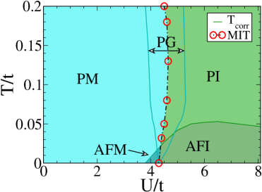
Figure 1: $U-T$ phase diagram of the Hubbard model at $t^{\prime}/t=0.8$. The phases are paramagnetic metal (PM), paramagnetic insulator (PI), antiferromagnetic metal (AFM) and antiferromagnetic insulator (AFI). The AFM and AFI are not simple Neel ordered. PG indicates a pseudogap phase, metallic or insulating. There is no genuine magnetic transition in two dimensions so our $T_{corr}$ indicates the temperature where the magnetic correlation length becomes larger than the system size $24\times 24$. The MIT line is determined from change in sign of the temperature derivative of resistivity, i.e, $d\rho/dT=0$.

To provide a quick background, there have been several studies of the single band Hubbard model on a triangular latticeth-hubb-Imada ; th-hubb-Ino ; th-hubb-Kawa ; th-hubb-Becca ; th-hubb-Lime ; th-hubb-Scale ; th-hubb-Phillips ; th-hubb-Kotl1 ; th-hubb-Ohashi ; th-hubb-Liebsch ; th-hubb-Sato ; th-hubb-Senech ; th-hubb-Mila to model organic physics. Dynamical mean field theory (DMFT) has been the method of choice th-hubb-Lime ; th-hubb-Scale ; th-hubb-Phillips , usually used in its cluster variant (C-DMFT) th-hubb-Kotl1 ; th-hubb-Ohashi ; th-hubb-Liebsch ; th-hubb-Sato to handle short range spatial correlations. The results depend on the degree of frustration and the specific method but broadly suggest the following: (i) the ground state is a PM Fermi liquid at weak coupling, a ‘spin liquid’ PI at intermediate coupling, and an AFI at large couplingth-hubb-Imada ; th-hubb-Ino ; th-hubb-Kawa ; th-hubb-Becca , (ii) the qualitative features in optics org-opt1 and transport th-hubb-Lime are recovered, (iii) there could be a re-entrant insulator-metal-insulator transition with increasing temperature for a certain window of frustration th-hubb-Ohashi ; th-hubb-Liebsch , (iv) the low temperature SC state could emerge th-hubb-org-sc1 ; th-hubb-org-sc2 ; th-hubb-org-sc3 from Hubbard physics, although there is no consensus th-hubb-org-sc-maz .

Surprisingly, there seems to be limited effort on the nature of spatial fluctuations, which could be significant in this low dimensional frustrated system. To clarify this aspect we study the single band Hubbard model on the anisotropic triangular lattice:

$$H=\sum_{\langle ij\rangle\sigma}t_{ij}c^{\dagger}_{i\sigma}c_{j\sigma}-\mu\sum_{i}n_{i}+U\sum_{i}n_{i\uparrow}n_{i\downarrow}$$ (1)

We use a square lattice geometry but with the following anisotropic hopping: $t_{ij}=-t$ when ${\bf R}_{i}-{\bf R}_{j}=\pm{\hat{x}}a_{0}$ or $\pm{\hat{y}}a_{0}$, where $a_{0}$ is the lattice spacing, and $t_{ij}=-t^{\prime}$ when ${\bf R}_{i}-{\bf R}_{j}=\pm({\hat{x}}+{\hat{y}})a_{0}$. We will set $t=1$ as the reference energy scale. $t^{\prime}=0$ corresponds to the square lattice, and $t^{\prime}=t$ to the isotropic triangular lattice. We have studied the problem over the entire $t^{\prime}/t$ window $[0,1]$, but focus on $t^{\prime}/t=0.8$ in this paper. $\mu$ controls the electron density, which we maintain at half-filling, $n=1$. $U>0$ is the Hubbard repulsion.

We use a Hubbard-Stratonovich (HS) transformation that introduces a vector field ${\bf m}_{i}(\tau)$ and a scalar field $\phi_{i}(\tau)$ at each site vec-hubb-hs1 ; vec-hubb-hs2 to decouple the interaction. We need two approximations to make progress. (i) We will treat the ${\bf m}_{i}$ and $\phi_{i}$ as classical fields, i.e, neglect their time dependence. (ii) While we completely retain the thermal fluctuations in ${\bf m}_{i}$, we treat $\phi_{i}$ at the saddle point level, i.e, $\phi_{i}\rightarrow\langle\phi_{i}\rangle=(U/2)\langle\langle n_{i}\rangle\rangle=U/2$ at half-filling. With this approximation the half-filled problem is mapped on to electrons coupled to the field ${\bf m}_{i}$ (see Supplement).

$$H_{eff}=\sum_{ij,\sigma}t_{ij}c^{\dagger}_{i\sigma}c_{j\sigma}-{\tilde{\mu}}N-\frac{U}{2}\sum_{i}{\bf m}_{i}\cdot\vec{\sigma}_{i}+\frac{U}{4}\sum_{i}{\bf m}_{i}^{2}$$ (2)

where ${\tilde{\mu}}=\mu-U/2$. We can write $H_{eff}=H_{el}\{{\bf m}_{i}\}+H_{cl}$, where $H_{cl}=(U/4)\sum_{i}{\bf m}_{i}^{2}$. For a given configuration $\{{\bf m}_{i}\}$ one just needs to diagonalise $H_{el}$, but the $\{{\bf m}_{i}\}$ themselves have to be determined from the distribution

$$P\{{\bf m}_{i}\}={{Tr_{c,c^{\dagger}}e^{-\beta H_{el}}e^{-\beta H_{cl}}}\over\int{\cal D}{\bf m}Tr_{c,c^{\dagger}}e^{-\beta H_{el}}e^{-\beta H_{cl}}}$$ (3)

Equation (2) describes electron propagation in the ${\bf m}_{i}$ background, while equation (3) describes how the ${\bf m}_{i}$ emerge and are spatially correlated due to electron motion. The neglect of dynamics in the ${\bf m}_{i}$ reduces the method to unrestricted Hartee-Fock (UHF) mean field theory at $T=0$. However, the exact inclusion of classical thermal fluctuations quickly improves the accuracy of the method with increasing temperature. We will discuss the limitations of the method further on.

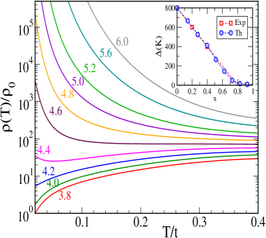
Figure 2: Temperature dependence of the resistivity for different $U$ in the neighbourhood of $U_{c}$. The normalising scale is $\rho_{0}={{\hbar}c_{0}}/{\pi e^{2}}$ (see text). This is $\sim 380\mu\Omega$cm for the organics. The $U/t$ values are indicated on the curves. The inset shows the experimental transport gap in the Cl_1-xBr_x family (in Kelvins), and our estimated transport gap. We used a fit $U(x)/t=6-1.35x-0.4x^{2}$ (see text) to reproduce the transport gaporg-res estimated from the experiments.

Due to the fermion trace, $P\{{\bf m}_{i}\}$ is not exactly calculable. To generate the equilibrium $\{{\bf m}_{i}\}$ we use MC sampling hs-mc-1 ; hs-mc-2 ; hs-mc-3 . Computing the energy cost of an attempted update requires diagonalising $H_{el}$. To access large sizes within limited time, we use a cluster algorithm tca for estimating the update cost. Rather than diagonalise the full $H_{eff}$ for every attempted update, we calculate the energy cost of an update by diagonalizing a small cluster (of size $N_{c}$, say) around the reference site. We have extensively benchmarked this cluster based MC methodtca . The MC was done for lattice of size $N=24\times 24$, with clusters of size $N_{c}=8\times 8$. We calculate the thermally averaged structure factor $S({\bf q})=\frac{1}{N^{2}}\sum_{ij}\langle{\bf m_{i}}\cdot{\bf m_{j}}\rangle e^{i{\bf q}\cdot({\bf R}_{i}-{\bf R}_{j})}$ at each temperature. The onset of rapid growth in $S({\bf q})$ at some ${\bf q}={\bf Q}$, say, indicates a magnetic transition. The electronic properties are calculated by diagonalising $H_{el}$ on the full lattice for equilibrium $\{{\bf m}_{i}\}$ configurations.

Fig.1 shows the $U-T$ phase diagram at $t^{\prime}/t=0.8$. Our low temperature result is equivalent to UHF and leads to a transition from an uncorrelated paramagnetic metal to an incommensurate AF metal with wavevector ${\bf Q}={\bf Q}_{1}\sim\{0.85\pi,0.85\pi\}$ at $U_{c1}\sim 4.0t$. At $U_{c2}\sim 4.5t$ there is a transition to an AF ‘Mott’ insulator with ${\bf Q}_{2}\sim\{0.8\pi,0.8\pi\}$. The magnitude $m_{i}=|{\bf m}_{i}|$ is small in the AFM and grows as $U/t$ increases in the Mott phase. The existence of the AF metal, and the nature of order in the intermediate $U/t$ Mott phase, could be affected by the neglected quantum fluctuations of the ${\bf m}_{i}$.

Finite temperature brings into play the low energy fluctuations of the ${\bf m}_{i}$. The effective model has the $O(3)$ symmetry of the parent Hubbard model so it cannot sustain true long range order at finite $T$. However, our annealing results suggest that magnetic correlations grow rapidly below a temperature $T_{corr}$, and weak interplanar coupling would stabilise in plane order below $T_{corr}$. This scale increases from zero at $U=U_{c1}$, reaches a peak at $U/t\sim 6.5$, and falls beyond as the virtual kinetic energy gain reduces with increasing $U$.

We classify the finite $T$ phases as metal or insulator based on $d\rho/dT$, the temperature derivative of the resistivity. The dotted line indicating the MIT corresponds to the locus $d\rho(T,U)/dT=0$. In addition to the magnetic and transport classification we also show a window around the MIT line where the electronic density of states (DOS) has a pseudogap. To the right of this region the DOS has a ‘hard gap’ while to the left it is featureless. The MIT line shows re-entrant insulator-metal-insulator behavior with increasing $T$ near $U\sim U_{c2}$.

We can attempt a quick comparison of the phase diagram with that in the $\kappa$-BEDT family. The primary hopping is $t\sim 65$meV, and $t^{\prime}/t\sim 0.8$ org-struct-hopping (a recent ab initio estimate suggests $t^{\prime}/t\lesssim 0.5$ for $\kappa$-Cl). Fitting the transport gap in $\kappa$-Cl (see Fig.1 inset) suggests that $U/t\sim 6.0$ at $x=0$. From our results this would indicate that $T_{corr}/t\sim 0.05$, at $x=0$, i.e, $T_{corr}\sim 35$K, not too far from the NMR inferred $T_{c}\sim 30$K.

Fig.2 shows the resistivity $\rho(T)$ computed via the Kubo formula for varying $U/t$. We first compute the planar resistivity (which has the dimension of resistance) and then compute the effective three dimensional resistivity of ‘decoupled’ layers (see Supplement) by using the $c$-axis spacing, $c_{0}$. In the Cl_1-xBr_x family it is observed that the transport gap can be fitted to $\Delta(x)\approx 800-1000x$ Kelvinorg-res . We match this to the $U$ dependence of our calculated gap, $\Delta(U)/t$, and infer $U/t|_{x=0}\sim 6$. The MIT occurs at $x_{c}\sim 0.75$ and for us at $U/t\approx 4.5$. Fitting a quadratic form to $U(x)/t$ to capture the measured transport gap, we get $U(x)/t\approx 6-1.35x-0.4x^{2}$. The $U/t$ range in Fig.2 corresponds roughly to $x=[0,1]$. Since $t=65$meV, $T=0.4t$ is approximately $300$K.

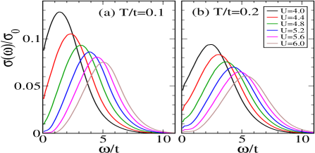
Figure 3: Optical conductivity at $T/t=0.1$ and $0.2$ for $U$ varying across $U_{c}$. At these temperatures the $\sigma(\omega)$ is non Drude even in the ‘weakly correlated’ case $U/t\sim 4.0$. The finite frequency peak evolves into the Hubbard transition at large $U/t$. For a rough comparison to organics, $T/t=0.1\equiv$80K, $\omega/t=5\equiv 2500$cm^-1, and $\sigma/\sigma_{0}=0.1\equiv 265\Omega^{-1}$cm^-1.

Our resistivity is in units of $\rho_{0}=\frac{\hbar c_{0}}{\pi e^{2}}$. Using $c_{0}\sim 29\AA$, $\rho_{0}\sim 380\mu\Omega$cm, yields $\rho\sim 60\rho_{0}\sim 25$m$\Omega$cm at $T\sim 0.4t$, while experimental value is $\gtrsim 100$m$\Omega$cm. The difference could come from electron-phonon scattering absent in our model. Limelette et alth-hubb-Lime presented DMFT based resistivity result that compares favourably with experiments, but, apparently, involves an arbitrary scale factor. Our re-entrant window $\delta U$=0.4$t$ near $U_{c}$, inferred from thermally driven I-M-I crossover, is equivalent to $\delta x$=0.2. This is consistent with $\delta x\sim 0.2$ in the Cl_1-xBr_x familyorg-res . The C-DMFT estimates of the re-entrant window varies widely, from $\delta U$$\sim$0.3$t$th-hubb-Liebsch to $\sim$1.2$t$th-hubb-Ohashi .

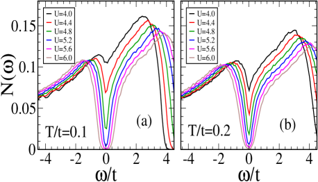
Figure 4: Density of states at $T/t=0.1,~{}0.2$ for $U$ varying across $U_{c}$. The dip in the DOS deepens with increasing $T$ for $U/t\lesssim 4.8$. For larger $U/t$ the system slowly gains spectral weight with increasing $T$.

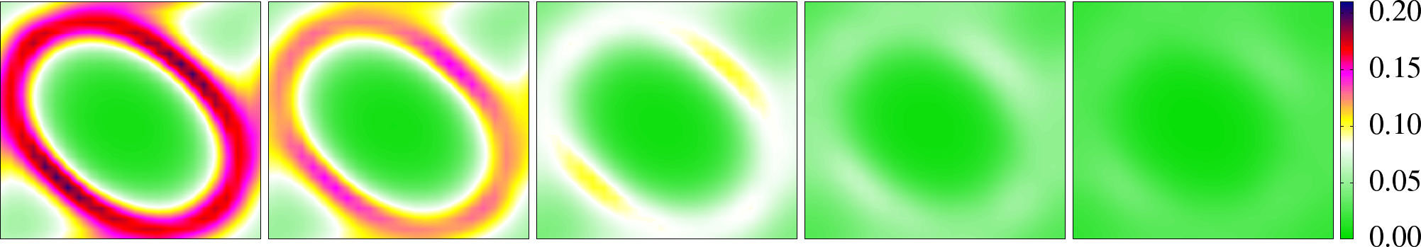
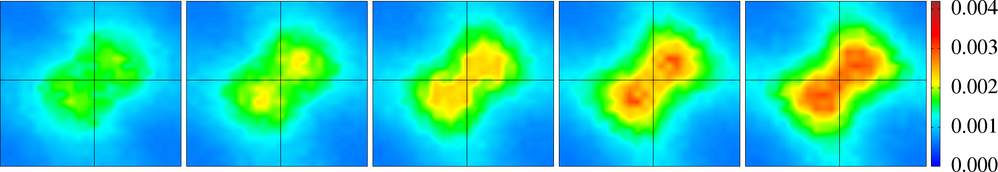
Figure 5: Top:  Momentum dependence of the low frequency spectral weight in the electronic spectral function $A({\bf k},\omega)$ at $T/t=0.1$. $k_{x},k_{y}$ range from [-$\pi,\pi$] in the panels. Note the systematically larger weight near ${\bf k}=[\pi/2,\pi/2]$ and $[-\pi/2,-\pi/2]$ and smaller weight in the segments near $[\pi,0]$ and $[0,\pi]$. $U/t=4.2,~{}4.4,~{}4.6,~{}4.8,~{}5.0$, left to right. Bottom:  Magnetic structure factor $S({\bf q})$ for the auxiliary fields ${\bf m}_{i}$ for the same set of $U/t$. The $q_{x},q_{y}$ range from $[0,2\pi]$. Note the very weak and diffuse structure at $U/t=4.2$ and the much larger and differentiated structure at $U/t=5.0$.

Fig.3 shows the optical conductivity $\sigma(\omega)$ at $T=0.1t$ and $T=0.2t$ as $U/t$ varied across the Mott crossover. Our first observation is the distinctly non Drude nature of $\sigma(\omega)$ in the metal, $U/t\lesssim 4.4$, with $d\sigma(\omega)/d\omega|_{\omega\rightarrow 0}>0$. The low frequency hump in the bad metal evolves into the interband Hubbard peak in the Mott phase. The change in the lineshape with increasing $T$ is more prominent in the metal, with the peak location moving outward, and is more modest deep in the insulator.

In the organics the experimenters have carefully isolated the Mott-Hubbard features in the spectrum by removing phononic and intra-dimer effects org-opt2 . Since we have already fixed our $t,t^{\prime},U$ we have no further fitting parameter for $\sigma(\omega)$. The measured spectrum at $x\sim x_{c}$ and $T\sim 50-90$K has a peak around $1500-2000$cm^-1. Using $U_{c}/t\sim 4.5$ and $T/t=0.1$ we get $\omega_{peak}/t\sim 3.0$, which translates to $\sim 1500$cm^-1. The magnitude of our $\sigma(\omega)$ at $\omega_{peak}$ is $\sim 0.1\sigma_{0}\sim 265\Omega^{-1}$cm^-1, since $\sigma_{0}=1/\rho_{0}\sim 2650\Omega^{-1}$cm^-1. This is remarkably close to the measured value, $\approx 280\Omega^{-1}$cm^-1(Ref. org-opt2 Fig.3).

While the characteristic scales in $\sigma(\omega)$ match well with experiments, the experimental spectrum has weaker dependence on temperature and composition $x$. This could arise from the subtraction process and the presence of other interactions in the real material. Our result differs from DMFT org-opt1 , and agrees with the experiments, in that we do not have any feature at $\omega=U/2$. We have verified the f-sum rule numerically.

The crossover from the bad metal to the insulator involves a wide window with a pseudogap in the electronic DOS, $N(\omega)$. One may have guessed this from the depleting low frequency weight in $\sigma(\omega)$, Fig.4 makes this feature explicit. We are not aware of tunneling studies in the organics, but our results indicate a wide window, $U/t\sim[4,5.3]$, where there is a distinct pseudogap in the global DOS. This suggests that the entire $x\sim[1.0,0.35]$ window in the organics should have a PG. For $U/t\lesssim 4.6$ the dip feature deepens with increasing $T$, we have $dN(0)/dT<0$ (compare panels (a) and (b), Fig.4), while for $U/t\gtrsim 4.6$ we have a weak $dN(0)/dT>0$. The PG arises from the coupling of electrons to the fluctuating ${\bf m}_{i}$. A large $m_{i}$ at all sites would open a Mott gap, independent of any order among the moments. Weaker $m_{i}$, thermally generated in the metal near $U_{c1}$ and with only short range correlations, manages to deplete low frequency weight without opening a gap. Since the typical size $\langle m_{i}\rangle$ increases with $T$ in the metal, we see the dip deepening at $U<U_{c}$.

While the size of the ${\bf m}_{i}$ determine the overall depletion of DOS near $\omega=0$ and the opening of the Mott gap, the angular correlations dictate the momentum dependence of the spin averaged electronic spectral function $A({\bf k},\omega)$ (see Supplement).

Within ‘local self energy’ picture, as in DMFT, $A({\bf k},\omega)$ should have no ${\bf k}$ dependence on the Fermi surface (FS). In that case we should have ${\bf k}$ independent suppression of $A({\bf k},0)$ with increasing $U/t$.

Fig.5, top row, shows maps of $A({\bf k},0)$ for $k_{x},k_{y}=[-\pi,\pi]$, at $T/t=0.1$, as increasing $U/t$ transforms the bad metal to a Mott insulator. The first panel at $U/t=4.2$ (roughly a Br sample) shows weak anisotropy on the nominal FS while Fig.4.(a) suggests that a weak PG has already formed. At $U/t=4.4$, next panel, the weak anisotropy is much amplified and the weight in the $[0,0]\rightarrow[\pi,\pi]$ direction is distinctly larger. The next three panels basically show insulating states but without a hard Mott gap. Overall, the ‘destruction’ of the FS seems to start near $[\pi,-\pi]$, the ‘hot’ region, and ends with the region near $[\pi/2,\pi/2]$, the ‘cold spot’. We show data on the full $A({\bf k},\omega)$ in the Supplement that indicates that with increasing $U$ a PG feature forms at the hot spot while the cold spot still has a quasiparticle peak.

Second row in Fig.5 shows the $S({\bf q})$ of the auxiliary fields at $T/t=0.1$ for the same $U/t$ as in the upper row. While there is no magnetic order we can see the growth of correlations centered around ${\bf Q}\approx[0.85\pi,0.85\pi]$ as $U/t$ increases. The dominant electron scattering would be from ${\bf k}$ to ${\bf k}+{\bf Q}$, and the impact would be greatest in regions of the FS in the proximity of minima in $|\nabla\epsilon_{\bf k}|$. The location of the hot spots on the FS, and the momentum connecting them, indeed correspond to this scenario.

While we have a method that captures non trivial spatial correlations and its impact on electronic properties, we need to be cautious about some shortcomings. (i) Neglecting the dynamics of the ${\bf m}_{i}$ misses correlation effects in the ground state of the metal and underestimates $U_{c}/t$. (ii) It also misses the ‘Fermi liquid’ physics in the low $T$ metal, but should be reliable in the $T/t\gtrsim 0.1$ regime that we have focused on. (iii) There is potentially a ‘spin liquid’ insulator th-hubb-Senech ; th-hubb-Mila at intermediate $U/t$ and $t^{\prime}/t=1$. We do not know of such results at $t^{\prime}/t=0.8$, but would prefer to emphasize our finite $T$ results rather than the nature of the ground state.

Conclusion: We introduced and explored in detail a method which retains the spatial correlations that are crucial near the Mott transition on a frustrated lattice. Using electronic parameters that describe the $\kappa$-BEDT based organics we obtain a magnetic $T_{c}$, metal-insulator phase diagram, and optical response that reproduces the key experimental scales. We uncover a wide pseudogap regime near the MIT, and predict distinct signatures of the incommensurate magnetic fluctuations in the angle resolved photoemission spectrum.

We acknowledge use of the HPC clusters at HRI. PM acknowledges support from the DST India (Athena), a DAE-SRC Outstanding Research Investigator grant, and a discussion with T. V. Ramakrishnan.

I Supplementary information:

I.1 Derivation of the effective Hamiltonian

Our starting point is the Hubbard model

$$H = \sum_{\langle ij\rangle\sigma}t_{ij}c^{\dagger}_{i\sigma}c_{j\sigma}-\mu\sum_{i}n_{i}+U\sum_{i}n_{i\uparrow}n_{i\downarrow}$$

$$= H_{0}-\mu\sum_{i}n_{i}+U\sum_{i}n_{i\uparrow}n_{i\downarrow}$$

We implement a rotation invariant decoupling of the Hubbard interaction as follows. First, one can write

$$n_{i\uparrow}n_{i\downarrow}=\frac{n_{i}^{2}}{4}-(\vec{s}_{i}\cdot{\hat{\bf m}_{i}})^{2}$$

where $n_{i}=n_{i\uparrow}+n_{i\downarrow}$ is the charge density, $\vec{s}_{i}=\frac{1}{2}\sum_{\alpha,\beta}c^{\dagger}_{i\alpha}\vec{\sigma}_{\alpha\beta}c_{i\beta}=2\vec{\sigma}_{i}$ is the local electron spin operator, and ${\hat{\bf m}_{i}}$ is an arbitrary unit vector.

The partition function of the Hubbard model is

$$Z = \int D[c,\bar{c}]e^{-S}$$ (5)

$$S = \int_{0}^{\beta}d\tau{\cal L}(\tau)$$ (6)

$${\cal L} = \sum_{i\sigma}\bar{c}_{i\sigma}(\tau)\partial_{\tau}c_{i\sigma}(\tau)+H(\tau)$$

We can introduce two space-time varying auxiliary fields for a Hubbard-Stratonovich transformation: (i) $\phi_{i}(\tau)$ coupling to charge density, and (ii) $\Delta_{i}(\tau){\hat{\bf m}_{i}}(\tau)={\bf m}_{i}(\tau)$ coupling to electron spin density ($\Delta_{i}$ is real positive). This allows us to define a SU(2) invariant HS transformation (see ref. [1, 2]),

$$e^{Un_{i\uparrow}n_{i\downarrow}}=\int\frac{d\phi_{i}d{\bf m}_{i}}{4\pi^{2}U}e^{\left(\frac{\phi_{i}^{2}}{U}+i\phi_{i}n_{i}+\frac{\bf{m}_{i}^{2}}{U}-2{\bf m}_{i}\cdot\vec{s}_{i}\right)}$$

The partition function now becomes:

$$Z = \int\prod_{i}\frac{d\bar{c_{i}}dc_{i}d\phi_{i}d{\bf m}_{i}}{4\pi^{2}U}e^{\left(-\int_{0}^{\beta}{\cal L}(\tau)\right)}$$ (7)

$${\cal L}(\tau) = \sum_{i\sigma}\bar{c}_{i\sigma}(\tau)\partial_{\tau}c_{i\sigma}(\tau)+H_{0}(\tau)+{\cal L}_{int}(\phi_{i}(\tau),{\bf m}_{i}(\tau))$$ (8)

$${\cal L}_{int} = \sum_{i}\left[\frac{\phi_{i}^{2}}{U}+i\phi_{i}n_{i}+{{\bf m}_{i}^{2}\over U}-2{\bf m}_{i}\cdot\vec{s}_{i}\right]$$

As discussed in the text, to make progress we need two approximations: (i) neglect the time ($\tau$) dependence of the HS fields, (ii) replace the field $\phi_{i}$ by its saddle point value $(U/2)\langle n_{i}\rangle=U/2$, since the important low energy fluctuations arise from the ${\bf m}_{i}$. Substituting these, and simplifying the action, one gets the effective Hamiltonian

$$H_{eff}=H_{0}-{\tilde{\mu}}\sum_{i}n_{i}-\sum_{i}{\bf m}_{i}\cdot\vec{\sigma}_{i}+\sum_{i}{{\bf m}_{i}^{2}\over U}$$

where ${\tilde{\mu}}=\mu-U/2$. For convenience we redefine ${\bf m}_{i}\rightarrow\frac{U}{2}{\bf m}_{i}$, so that the ${\bf m}_{i}$ is dimensionless. This leads to the effective Hamiltonian used in the text:

$$H_{eff}=H_{0}-{\tilde{\mu}}\sum_{i}n_{i}-{U\over 2}\sum_{i}{\bf m}_{i}\cdot\vec{\sigma}_{i}+{U\over 4}\sum_{i}{\bf m}_{i}^{2}$$

The partition function can be written as:

$$Z=\int{\cal D}{\bf m}_{i}Tr_{c,c^{\dagger}}e^{-\beta H_{eff}}$$

For a given configuration $\{{\bf m}_{i}\}$ the problem is quadratic in the fermions, while the configurations themselves are obtained by a Monte Carlo as discussed in the text.

I.2 Optical conductivity

The conductivity of the two dimensional system is first calculated as follows (ref.[3]), using the Kubo formula:

$$\sigma_{2D}^{xx}(\omega) = \frac{\sigma_{0}}{N}\sum_{\alpha,\beta}{{n_{\alpha}-n_{\beta}}\over{\epsilon_{\beta}-\epsilon_{\alpha}}}|\langle\alpha|J_{x}|\beta\rangle|^{2}\delta(\omega-(\epsilon_{\beta}-\epsilon_{\alpha}))$$

Where, the current operator $J_{x}$ is

$$J_{x} = -i\sum_{i,\sigma}\left[t(c^{\dagger}_{i,\sigma}c_{i+\hat{x},\sigma}-\textrm{hc})+t^{\prime}(c^{\dagger}_{i,\sigma}c_{i+\hat{x}+\hat{y},\sigma}-\textrm{hc})\right]$$

The d.c conductivity is the $\omega\rightarrow 0$ limit of the result above. $\sigma_{0}$=$\frac{\pi e^{2}}{\hbar}$, the scale for two dimensional conductivity, has the dimension of conductance. $n_{\alpha}=f(\epsilon_{\alpha})$ is the Fermi function, and $\epsilon_{\alpha}$ and $|\alpha\rangle$ are respectively the single particle eigenvalues and eigenstates of $H_{eff}$ in a given background {${\bf m}_{i}$}. The results we show in the text are averaged over equilibrium MC configurations.

The experimental results are quoted as resistivity of a three dimensional material. If we assume that the planes are electronically decoupled, as we have done in the text, then the three dimensional resistivity $\rho_{3D}$ can be estimated from the resistance of a cube of size $L^{3}$. If the 2D resistivity is $\rho_{2D}=1/\sigma_{2D}$, the resistance of a $L^{2}$ sheet is just $\rho_{2D}$ itself. A stacking of such sheets, with spacing $c_{0}$ in the third direction, implies that the resistance of the $L^{3}$ system would be $R_{3D}=\rho_{2D}c_{0}/L$. By definition this also equals $\rho_{3D}L/L^{2}=\rho_{3D}/L$. Equating the two, $\rho_{3D}=\rho_{2D}c_{0}$.

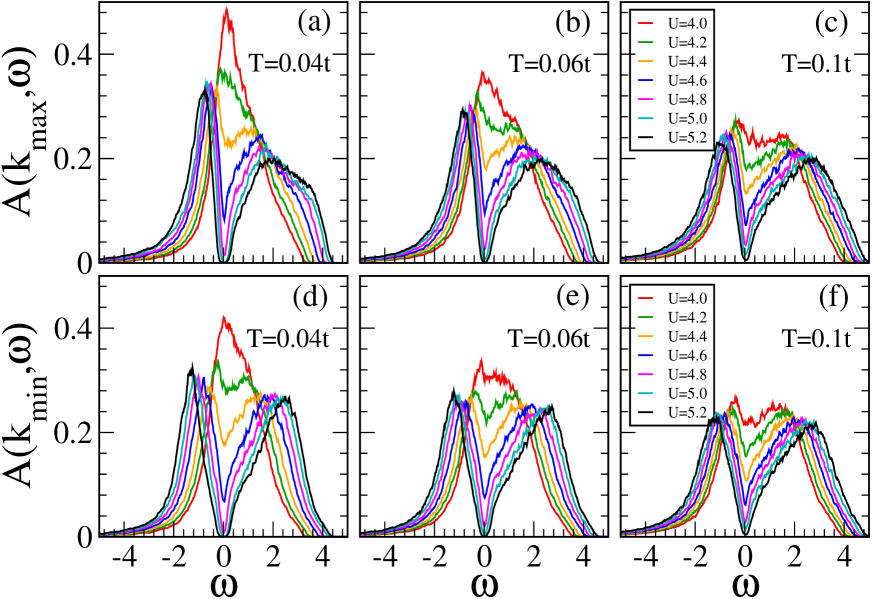
Figure 6: The spectral function $A({\bf k},\omega)$ at two ${\bf k}$ points on the FS that correspond to the highest and lowest value of $A({\bf k},0)$. We highlight the anisotropy over a range of $U/t$ values, as the system evolves from a moderately damped metal to a pseudogap phase, and three temperatures.

I.3 Spectral function

We extract the thermal and spin averaged spectral function $A({\bf k},\omega)$ as follows. First, the retarded Greens function

$$G_{\sigma}({\bf k},t)=-i\theta(t)\langle\{c_{{\bf k}\sigma}(t),c^{\dagger}_{{\bf k}\sigma}(0)\}\rangle$$

which can be simplified to

$$G_{\sigma}({\bf k},t)=-i\theta(t)\sum_{\alpha}|\langle{\bf k}\sigma|\alpha\rangle|^{2}e^{-i\epsilon_{\alpha}t}$$

where $\{|\alpha\rangle\}$ are the single particle eigenstates and $\epsilon_{\alpha}$ are eigenvalues in a given $\{{\bf m}_{i}\}$ background. In frequency domain, this becomes

$$G_{\sigma}({\bf k},\omega)=\sum_{\alpha}\frac{|\langle{\bf k}\sigma|\alpha\rangle|^{2}}{\omega-\epsilon_{\alpha}+i0^{+}}$$

From this: $A_{\sigma}({\bf k},\omega)=-{1\over\pi}$ Im$G_{\sigma}({\bf k},\omega)$ is simply $\sum_{\alpha}|\langle{\bf k}\sigma|\alpha\rangle|^{2}\delta(\omega-\epsilon_{\alpha})$. We average this over spin orientations, $\sigma$, and over thermal configurations. The ${\bf k}$ dependent weight at $\omega=0$ is shown in Fig.5 in the text. The full spectral function at the ‘cold spot’ and ‘hot spot’, where $A({\bf k},0$ is maximum and minimum, are shown, respectively, in the top and bottom panels in the figure 6.

We have averaged the spectrum over the four ${\bf k}$ neighbours of the nominal ‘cold’ and ‘hot’ points of our $24\times 24$ lattice. This averaging reduces the anisotropy, so the true anisotropy would be greater than what we show here. Also note that at $T=0.1t$, where the $A({\bf k},0)$ in the text is shown, the spectral function has no peak at $\omega=0$ either in the cold or hot spot. The pseudogap feature is visible all over the FS even at $U/t=4$.

References

- [1] N. F. Mott, Metal-Insulator Transitions, Taylor and Francis (1990).
- [2] A. Georges, G. Kotliar, W. Krauth and M. J. Rozenberg, Rev. Mod. Phys. 68 13 (1996).
- [3] M. Imada, A. Fujimori and Y. Tokura, Rev. Mod. Phys. 70 1039 (1998)
- [4] E. Dagotto, Rev. Mod. Phys. 66, 763 (1994).
- [5] N. P. Ong and R. J. Cava, Science 305 52 (2005).
- [6] L. Balents, Nature 464 199 (2010).
- [7] K. Kanoda and R. Kato, Annu. Rev. Condens. Matter Physics. 2 167 (2011).
- [8] B. J. Powell and R. H. McKenzie Rep. Prog. Phys. 74, 056501 (2011).
- [9] H. C. Kandpal, et al., Phys. Rev. Lett. 103 067004 (2009), Y. Shimizu, M. Maesato and G. Saito, J. Phys. Soc. Jpn. 80 074702 (2011).
- [10] S. Lefebvre, et al., Phys. Rev. Lett. 85 5420 (2000), F. Kagawa, T. Itou, K. Miyagawa, and K. Kanoda, Phys. Rev. B. 69 064511 (2004).
- [11] S. Yasin, et al., Eur. Phys. J. B. 79 383 (2011).
- [12] J. Merino, et al., Phys. Rev. Lett. 100 086404 (2008).
- [13] M. Dumm, et al., Phys. Rev. B. 79 195106 (2009).
- [14] B. J. Powell, E. Yusuf, and R. H. McKenzie, Phys. Rev. B. 80 054505 (2009).
- [15] A. Kawamoto, K. Miyagawa, Y. Nakazawa, and K. Kanoda, Phys. Rev. B. 52 15522 (1995).
- [16] H. Morita, S.Watanabe and M. Imada, J. Phys. Soc. J 71 2109 (2002).
- [17] T. Watanabe, H. Yokoyama, Y. Tanaka, and J. Inoue, Phys. Rev. B 77 214505 (2008).
- [18] K. Inaba, A. Koga, S. Suga, and N. Kawakami, J. Phys.: Conf. Ser. 150 042066 (2009), T. Yoshioka, A. Koga and N. Kawakami, Phys. Rev. Lett. 103 036401 (2009).
- [19] L. F. Tocchio, A. Parola, C. Gros, and F. Becca, Phys. Rev. B 80 064419 (2009).
- [20] P. Limelette, et al., Phys. Rev. Lett. 91 016401 (2003).
- [21] K. Aryanpour, W. E. Pickett, and R. T. Scalettar, Phys. Rev. B. 74 085117 (2006).
- [22] D. Galanakis, T. D. Stanescu and P. Phillips, Phys. Rev. B. 79 115116 (2009).
- [23] O. Parcollet, G. Biroli and G. Kotliar, Phys. Rev. Lett. 92, 226402 (2004).
- [24] T. Ohashi, T. Momoi, H. Tsunetsugu, and N. Kawakami, Phys. Rev. Lett. 100 076402 (2008).
- [25] A. Liebsch, H. Ishida, and J. Merino, Phys. Rev. B. 79 195108 (2009).
- [26] T. Sato, K. Hattori and H. Tsunetsugu, J. Phys. Soc. Jpn. 81 083703 (2012).
- [27] P. Sahebsara and D. Senechal, Phys. Rev. Lett. 100, 136402 (2008).
- [28] H. Y. Yang, A. M. Lauchli, F. Mila and K. P. Schmidt, Phys. Rev. Lett. 105, 267204 (2010).
- [29] T. Watanabe, H. Y. Okoyama, Y. Tanaka and J. Inoue, J. Phys. Soc. Jpn. 75 074707 (2006).
- [30] B. Kyung and A.-M. S. Tremblay, Phys. Rev. Lett. 97 046402 (2006).
- [31] J. Liu, J. Schmalian, and N. Trivedi, Phys. Rev. Lett. 94, 127003 (2005).
- [32] R. T. Clay, H. Li, and S. Mazumdar, Phys. Rev. Lett. 101, 166403 (2008).
- [33] J. Hubbard, Phys. Rev. Lett. 3 77 (1959).
- [34] H. J. Schulz, Phys. Rev. Lett. 65 2462 (1990).
- [35] M. Mayr, G. Alvarez, A. Moreo, and E. Dagotto, Phys. Rev. B. 73 014509 (2006).
- [36] E. Dagotto and T. Hotta and A. Moreo, Phys. Rep. 344 1 (2001).
- [37] Y. Dubi, Y. Meir and Y. Avishai, Nature, 449, 876 (2007).
- [38] S. Kumar and P. Majumdar, Eur. Phys. J. B, 50, 571 (2006).

References

- [1] Weng, Z. Y. and Ting, C. S. and Lee, T. K., Phys. Rev. B 43 3790 (1991)
- [2] K. Borejsza and N. Dupuis, Europhys. Lett. 63 722 (2003)
- [3] P. B. Allen in Conceptual Foundation of Materials V.2, edited by Steven G. Louie, Marvin L. Cohen, Elsevier (2006).